Article

Induction Motor Fault Diagnosis Using Low-Cost MEMS Acoustic Sensors and Multilayer Neural Networks

School of Electronic and Electrical Engineering, Kyungpook National University, Daegu 41566, Republic of Korea
*
Author to whom correspondence should be addressed.
Appl. Sci. 2025, 15(17), 9379; https://doi.org/10.3390/app15179379 (registering DOI)
Submission received: 5 August 2025 / Revised: 21 August 2025 / Accepted: 22 August 2025 / Published: 26 August 2025
(This article belongs to the Special Issue Artificial Intelligence in Machinery Fault Diagnosis)

Abstract

Induction motors are the dominant choice in industrial applications due to their robustness, structural simplicity, and high reliability. However, extended operation under extreme conditions, such as high temperatures, overload, and contamination, accelerates the degradation of internal components and increases the likelihood of faults. These faults are challenging to detect, as they typically develop gradually without clear external indicators. To address this issue, the present study proposes a cost-effective fault diagnosis system utilizing low-cost MEMS acoustic sensors in conjunction with a lightweight multilayer neural network (MNN). The same MNN architecture is employed to systematically compare three types of input feature representations: raw time-domain waveforms, FFT-based statistical features, and PCA-compressed FFT features. A total of 5040 samples were used to train, validate, and test the model for classifying three conditions: normal, rotor fault, and bearing fault. The time-domain approach achieved 90.6% accuracy, misclassifying 102 samples. In comparison, FFT-based statistical features yielded 99.8% accuracy with only two misclassifications. The FFT + PCA method produced similar performance while reducing dimensionality, making it more suitable for resource-constrained environments. These results demonstrate that acoustic-based fault diagnosis provides a practical and economical solution for industrial applications.

1. Introduction

Induction motors are known for their robustness, high reliability, and structural simplicity [1,2]. These characteristics have established them as the dominant choice across a wide range of industrial sectors [3,4]. In typical applications, induction motors operate under harsh conditions, including high temperatures, overload conditions, and contaminated environments [5,6,7]. Such conditions accelerate the deterioration of internal components during prolonged operation, increasing the likelihood of faults [8,9]. Given the extensive industrial reliance on induction motors, these faults can lead to serious consequences across various sectors [10,11]. Unexpected motor failures may result in costly repairs, production delays, and even safety hazards [12,13,14]. When used as critical components in industrial systems, such failures can significantly compromise overall system efficiency and productivity. Consequently, accurate fault classification methods are essential for timely maintenance and minimizing economic losses.
Induction motor faults are primarily categorized as either mechanical or electrical, based on their underlying mechanisms [15]. Electrical failures include stator winding faults, insulation breakdowns, and voltage imbalances [16,17,18]. Mechanical failures, in contrast, include bearing wear, rotor bar damage, and shaft misalignment [19,20,21]. This study focuses specifically on mechanical faults, namely bearing and rotor faults. Bearing faults represent more than 40% of all induction motor failures, whereas rotor faults account for approximately 10% [22]. These internal faults are difficult to detect visually and often result in sudden, unexpected breakdowns. Therefore, reliable fault diagnosis is essential to reduce maintenance costs and avoid production disruptions.
To achieve reliable fault diagnosis, existing studies have explored various sensor types and artificial intelligence techniques [23,24,25,26,27]. Toma et al. [28] used motor current signals to diagnose bearing faults, utilizing a genetic algorithm (GA) for feature selection and three machine learning classifiers: K-nearest neighbors (KNN), decision trees, and random forests. In vibration-based approaches, Tran et al. [29] converted vibration signals into time–frequency images using continuous wavelet transform (CWT) and applied an attention-based convolutional neural network (CANN) for fault classification. Building on vibration analysis, You et al. [30] proposed a hybrid deep neural model using raw vibration signals, integrating principal component analysis (PCA), convolutional neural networks (CNNs), bidirectional long short-term memory (BiLSTM), and an attention mechanism for rolling bearing fault diagnosis. Using a different sensor type, Choudhary et al. [31] employed infrared thermography combined with 2D discrete wavelet transform (DWT) for bearing fault detection, comparing classifiers including classification and decision trees (CDTs), linear discriminant analysis (LDA), and support vector machines (SVMs). For acoustic-based approaches, Germen et al. [32] used multiple microphones to detect both mechanical and electrical faults, applying self-organizing maps (SOMs) and learning vector quantization (LVQ) with correlation and wavelet transform (WT) analysis.
Previous methods typically involve complex signal processing, computationally demanding algorithms, and expensive equipment. In contrast, this study proposes an efficient and practical approach using low-cost MEMS acoustic sensors and lightweight models. A physical shielding structure is implemented to minimize acoustic interference. The acquired signals are preprocessed using conventional signal processing techniques to extract features for fault classification. A lightweight multilayer neural network (MNN) is employed to balance accuracy with computational efficiency. Additionally, three input feature representation methods are compared to evaluate their impact on diagnostic performance:
  • Time-domain (raw waveform): Preserves complete temporal information but may retain noise unrelated to fault diagnosis.
  • Frequency-domain statistical features (FFT-based): Statistical features such as mean, variance, median, skewness, and kurtosis are extracted from FFT-transformed signals to characterize the spectral distribution patterns.
  • Frequency domain PCA (FFT-based): PCA is applied to FFT-transformed signals to reduce dimensionality while preserving essential spectral characteristics.
This study focuses on practical applicability by adopting low-cost sensors, simple preprocessing, and a lightweight model. The remainder of this paper is organized as follows: Section 2 provides the theoretical background, Section 3 describes the proposed experimental setup and data acquisition, Section 4 presents the experimental results, and Section 5 concludes the study.

2. Theoretical Background

2.1. Input Data Preparation

2.1.1. Time Domain

The first input format is the raw time-domain signal, which retains the original waveform to preserve complete temporal information without any preprocessing. While this approach minimizes information loss, it is also vulnerable to noise, outliers, and redundant patterns that can hinder diagnostic accuracy. The raw time-domain signal x(t) is expressed as:
x t = s t + n ( t )
where s(t) represents the actual signal generated by the induction motor and n(t) denotes the environmental noise. The signal x(t) can be represented as a vector:
x t = [ x 1 , x 2 , , x T ] R T
where each element x i represents the signal amplitude at a specific time t i and T is the number of samples per second, corresponding to the sampling rate. In this approach, the entire vector x(t) is fed directly into the classifier without further preprocessing. Figure 1a–c show the acquired waveform data of the induction motor over a 0.1 s interval, corresponding to three motor conditions: (a) normal, (b) rotor fault, and (c) bearing fault.
In the normal condition, the amplitude variations remain relatively stable within a range of approximately −400 to +400. Under the rotor fault condition, certain segments exhibit slightly higher amplitudes; however, the overall waveform is largely comparable to that of the normal condition. This occurs because rotor bar damage modulates the motor noise slightly through torque variations at the slip frequency, rather than producing distinct impact events [33]. As a result, no clear distinction between the two conditions can be observed in the time domain. In contrast, the bearing fault condition is characterized by a much wider amplitude range of −3000 to +3000, along with repeated high-energy spikes. These features arise from periodic mechanical impacts caused by surface damage on the bearing, which generate abrupt changes in the short-term amplitude of the acoustic signal. Therefore, while bearing faults can be readily identified in the time domain, the normal and rotor fault conditions appear visually similar, indicating that effective rotor fault diagnosis requires a frequency spectrum-based approach.

2.1.2. Frequency Domain with Statistical Features

The second input format consists of statistical features derived from the frequency domain. To obtain these features, an FFT is applied to the acoustic signal. The discrete Fourier transform (DFT), implemented via FFT, is defined as [34]:
X k = n = 0 N 1 x n · e i 2 π k n k ,   k = 0,1 , , N 1
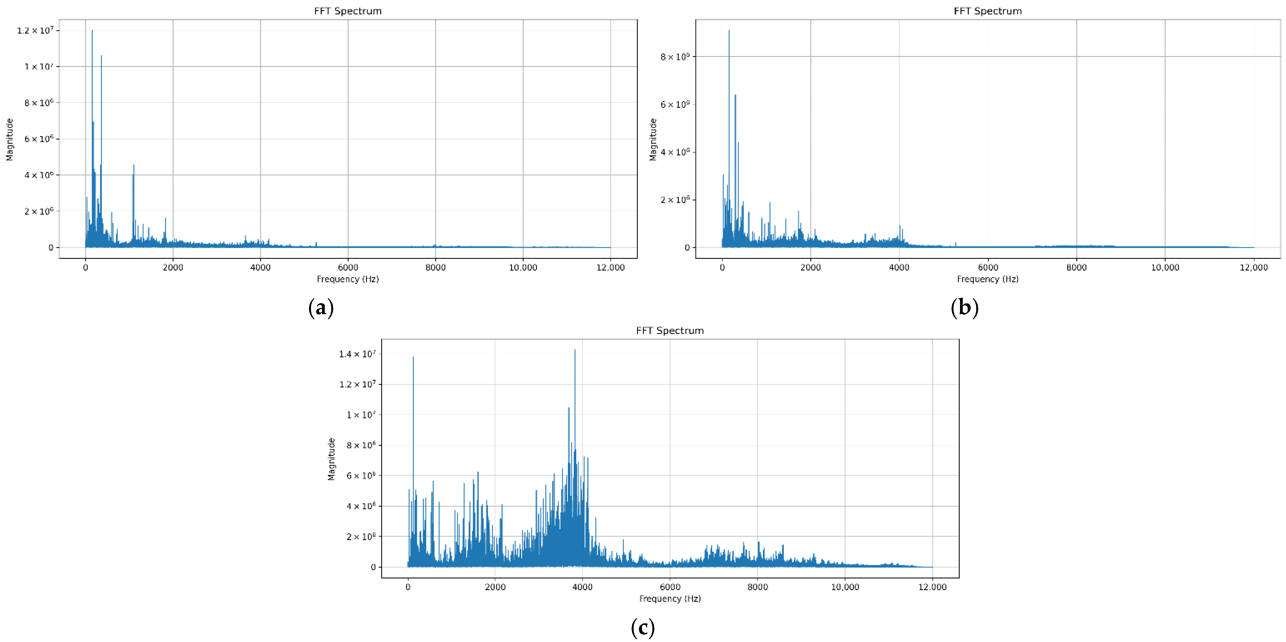
where x n is the input signal in the time domain, N is the total number of samples, and x k is the k-th frequency component, which is a complex-valued quantity. Figure 2a–c illustrate the frequency-domain spectra for the three states: normal, rotor fault, and bearing fault. In the normal state, a distinct peak distribution is observed in the 0–1 kHz range. In comparison, the rotor fault condition exhibits multiple small peaks irregularly distributed within the 1.5–4 kHz range. This irregularity can be attributed to rotor imbalance, torque pulsation, or subtle mechanical vibrations influencing the normal signal. The bearing fault condition, in contrast, shows increased broadband energy in the high-frequency range of 3–8 kHz, with a pronounced resonance component near 4 kHz. These high-frequency components result from impulsive vibrations caused by bearing surface damage or repetitive mechanical impacts that propagate across the frequency spectrum. This comparison demonstrates that faults difficult to distinguish in the time domain can be more clearly identified in the frequency domain. The presented spectrum was obtained by applying an FFT to the entire signal duration without the use of a window function. This approach is intended for visualization purposes, providing an overall view of the frequency component distribution across the entire signal rather than detailed analysis. By avoiding a window function, amplitude correction becomes unnecessary, and using the full signal length minimizes frequency resolution loss.
Table 1 presents the statistical features extracted from the frequency-domain data, along with their respective formulas [35,36,37]. The mean represents the average value of the spectral amplitude and indicates the dominant frequency region within the signal. The variance indicates dispersion of spectral energy around the average frequency. The median is the middle value of the sorted frequency components. As a central tendency indicator, it is less affected by outliers, providing a more stable basis for analysis than the mean [35]. Skewness measures the asymmetry of a frequency distribution to detect a bias toward a specific frequency region [38]. Kurtosis measures the tail sharpness of a distribution and the thickness of its tails [37].

2.1.3. Frequency Domain with PCA

The third input method employs PCA applied to frequency-domain data. First, the time-domain signal is transformed into the frequency domain using FFT. PCA is then used to extract a compact feature set from the transformed data. PCA is a widely used technique for dimensionality reduction [38]; it projects high-dimensional data into a lower-dimensional space while preserving as much of the original variance as possible.
The mathematical formulation used for PCA is given in Equation (4) [39].
C v i = λ i v i
where C denotes the covariance matrix representing the linear correlation between variables, v i is the i-th eigenvector, and λ i is the corresponding eigenvalue. The core process of PCA is to select the principal components associated with the largest eigenvalues. This process reduces the dimensionality of the data while minimizing information loss. The resulting feature set is then used as input to the classifier.

2.1.4. MNN

The same MNN classifier is applied across all three input types described above. An MNN typically consists of an input layer, one or more hidden layers, and an output layer. The forward propagation in the MNN is expressed by Equation (5):
y = σ ( W 2 σ W 1 x + b 1 + b 2 )
where x is an input feature vector, W n and b n are the weight matrix and bias vector of the n-th hidden layer, respectively, and σ is an activation function. MNNs achieve classification by performing nonlinear transformations across layers.
In this study, the model architecture includes two hidden layers. The ReLU activation function is used in the hidden layers to introduce nonlinearity, while the softmax function is applied at the output layer to generate class probabilities. The output layer has three nodes corresponding to the classification categories: normal, rotor fault, and bearing fault. The model is trained using the Adam optimizer and a cross-entropy loss function. The detailed network configuration and training parameters are presented in Table 2.

3. Proposed Experimental Setup and Data Acquisition

3.1. Experimental Methodology

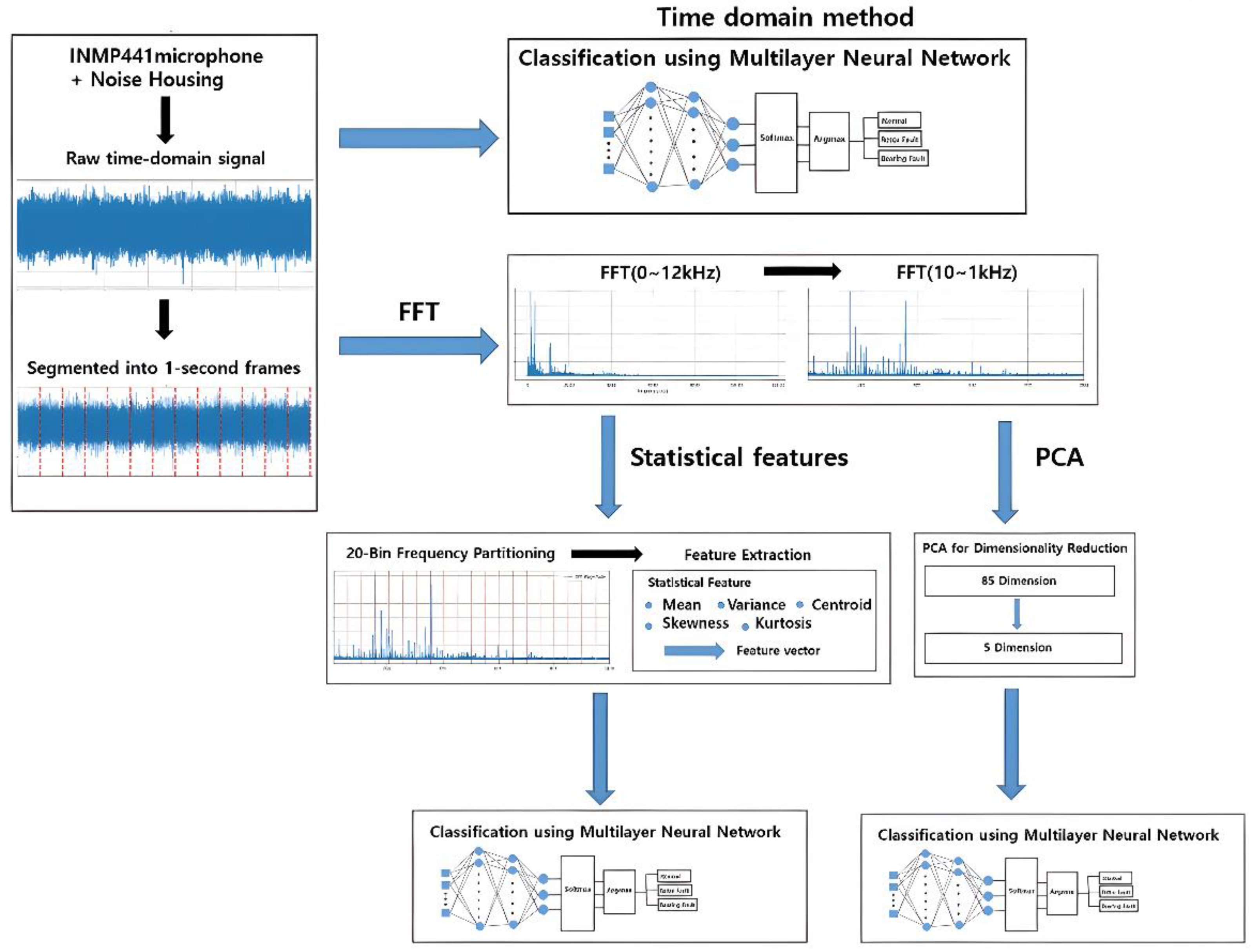
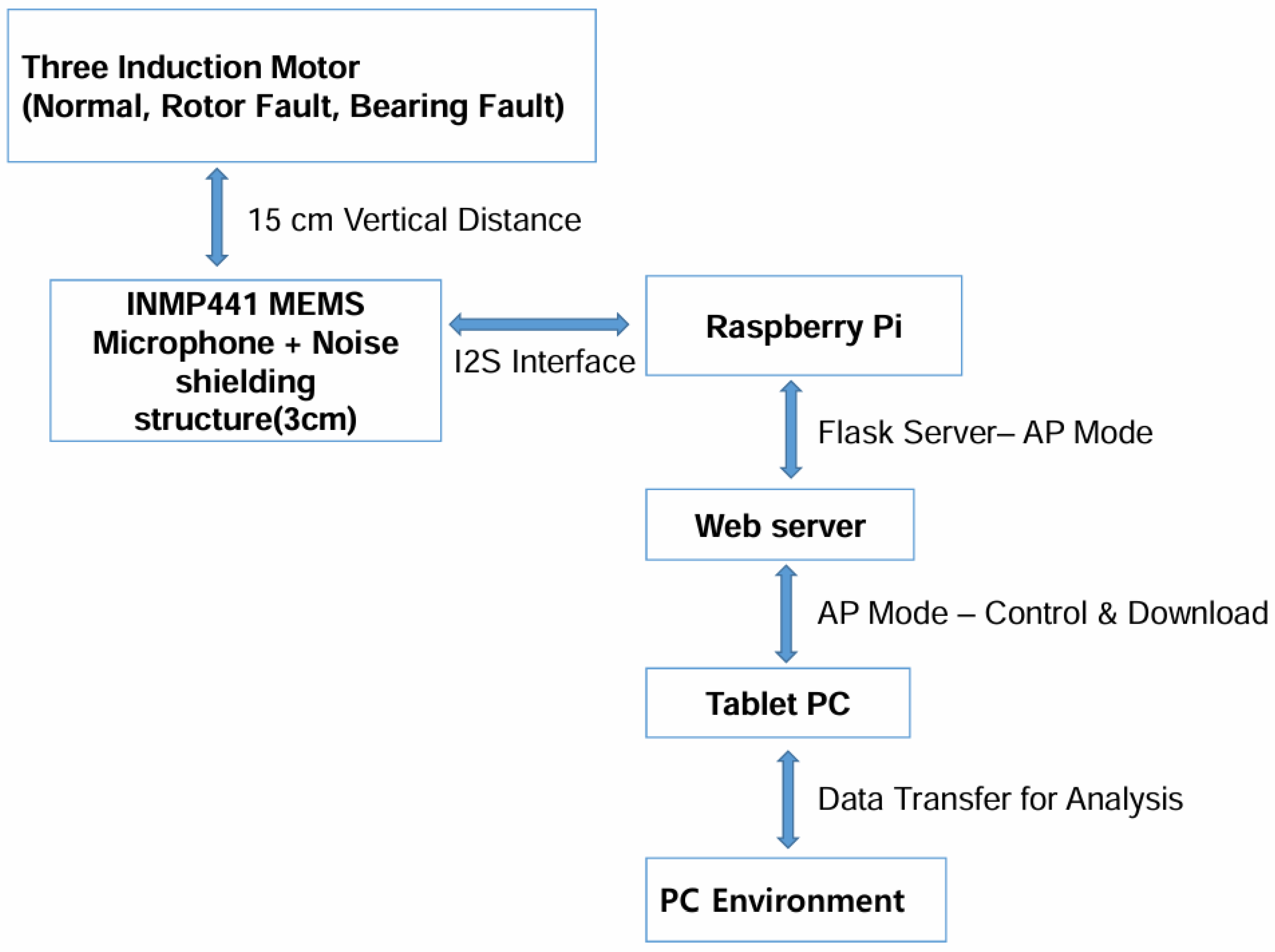
Figure 3 illustrates the overall experimental flow, which consists of four main steps: data acquisition, data preprocessing, feature extraction, and fault classification.
  • Data acquisition: An INMP441 acoustic sensor, equipped with a noise-shielding structure to minimize external interference, was used to collect acoustic data from an operating induction motor.
  • Data Preprocessing: The raw time-domain acoustic signals were divided into 1 s segments to construct the dataset.
  • Feature Extraction: Input features were generated using three distinct methods. The first method used raw time-domain data without preprocessing. The second method extracted statistical features from 20 uniformly spaced frequency bins. The third method applied PCA to the frequency-domain data to reduce dimensionality.
  • Fault Classification: Features extracted by the three methods were used as input to the MNN classifier. The classifier categorized each data segment into one of three classes: normal, rotor fault, or bearing fault.

3.2. Experimental Induction Motor and Fault Scenarios

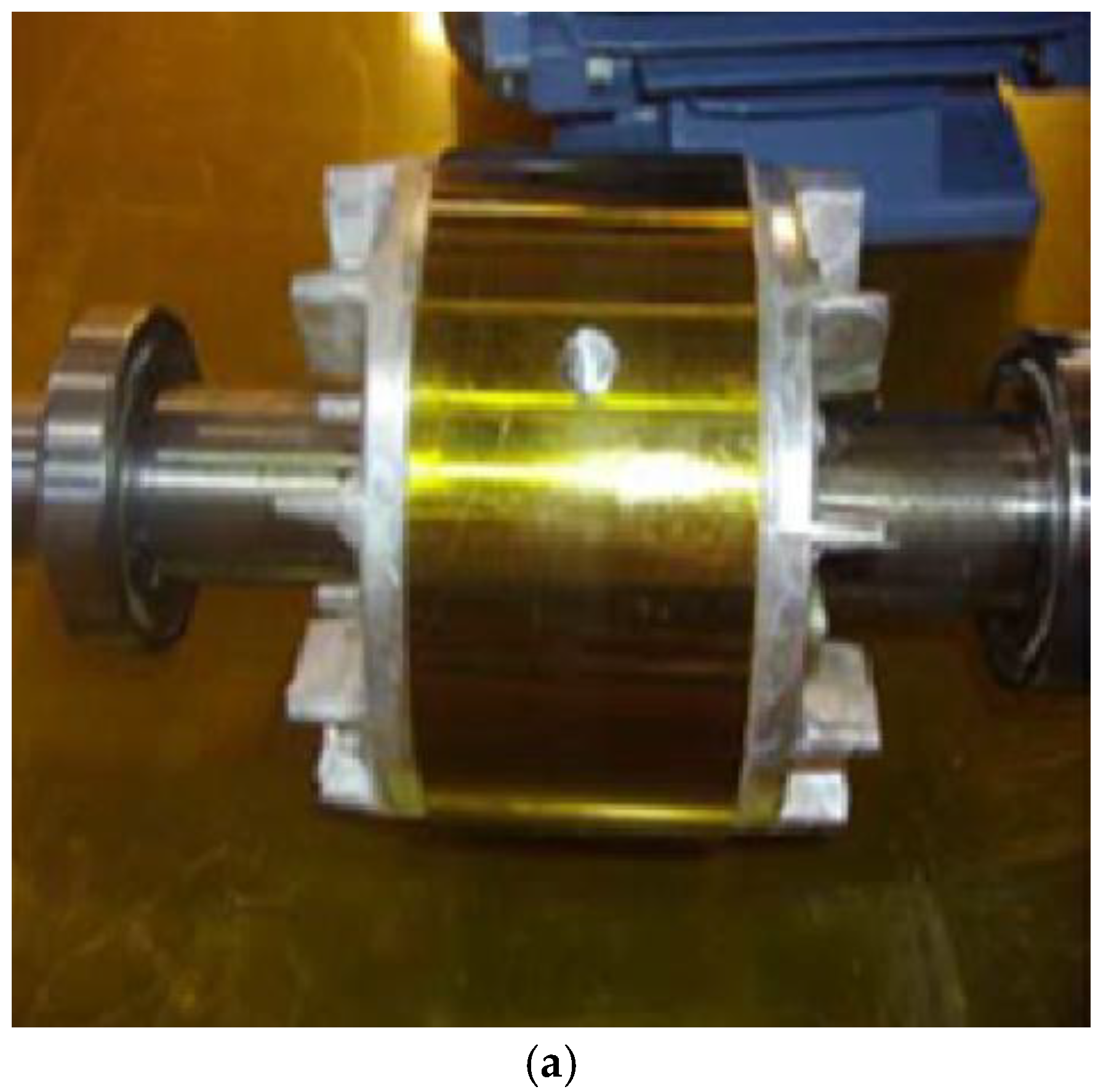
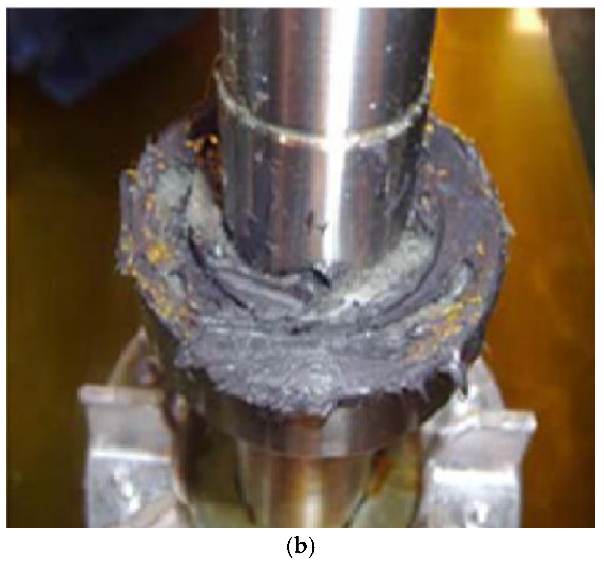
This experiment used a three-phase squirrel-cage induction motor, with its main specifications listed in Table 3. The motor operated at a rated voltage of 220/380 V and a frequency of 60 Hz, with a rated speed of 1730 rpm. An IP54 enclosure was used to protect the motor from dust and moisture. To ensure reliable operation, high-precision ball bearings were installed on both the load and non-load sides. The motor and load were connected via a V-belt and V-pulley system. Two types of faults were simulated in this study: a bearing fault and a rotor fault. The bearing fault was introduced by injecting iron powder into the bearing lubricant, as shown in Figure 4a, while the rotor fault was created by drilling a hole into the rotor bar, as illustrated in Figure 4b.

3.3. Acoustic Sensor Configuration and Noise Shielding Structure

The INMP441 MEMS microphone was selected for its robustness against electromagnetic interference (EMI), which is critical during motor operation. Its I2S digital interface helps minimize signal distortion caused by EMI. The microphone also provides a high signal-to-noise ratio (SNR) of 61 dBA and a wide frequency response range of 60 Hz to 15 kHz, sufficient to capture the primary frequency components associated with motor faults—all while remaining cost-effective. The detailed specifications are provided in Table 4.
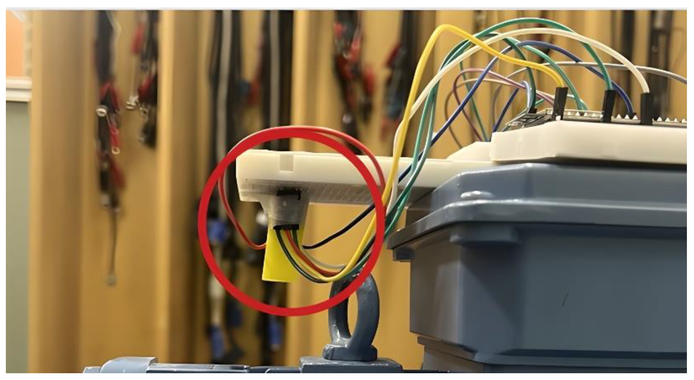
Despite its advantages, the omnidirectional nature of the sensor meant it also captured unwanted acoustic reflections from the floor, ceiling, and surrounding environment. To mitigate this, a noise-shielding structure was developed using a plastic tube. Figure 5 shows the shielding design.
This shielding setup helped filter out ambient and reflected noise, focusing instead on capturing the acoustic signals generated directly by the motor. Figure 6 presents a comparison of frequency distributions before and after the shielding was applied. The red line represents the unshielded configuration, and the blue line shows the shielded condition.
The sampling rate was 24 kHz, and the FFT length was set equal to the total number of samples in the signal. Since the objective was to visualize the overall distribution of frequency components, no segmentation or window function was applied. In the unshielded condition, strong components below 200 Hz were observed, attributed to environmental noise and acoustic reflections. After shielding was applied, these low-frequency noise components were significantly reduced, while the primary fault-related peaks in the mid- and high-frequency ranges were preserved. This demonstrates that the shielding effectively suppresses unwanted noise without compromising diagnostic information.

3.4. Data Acquisition System

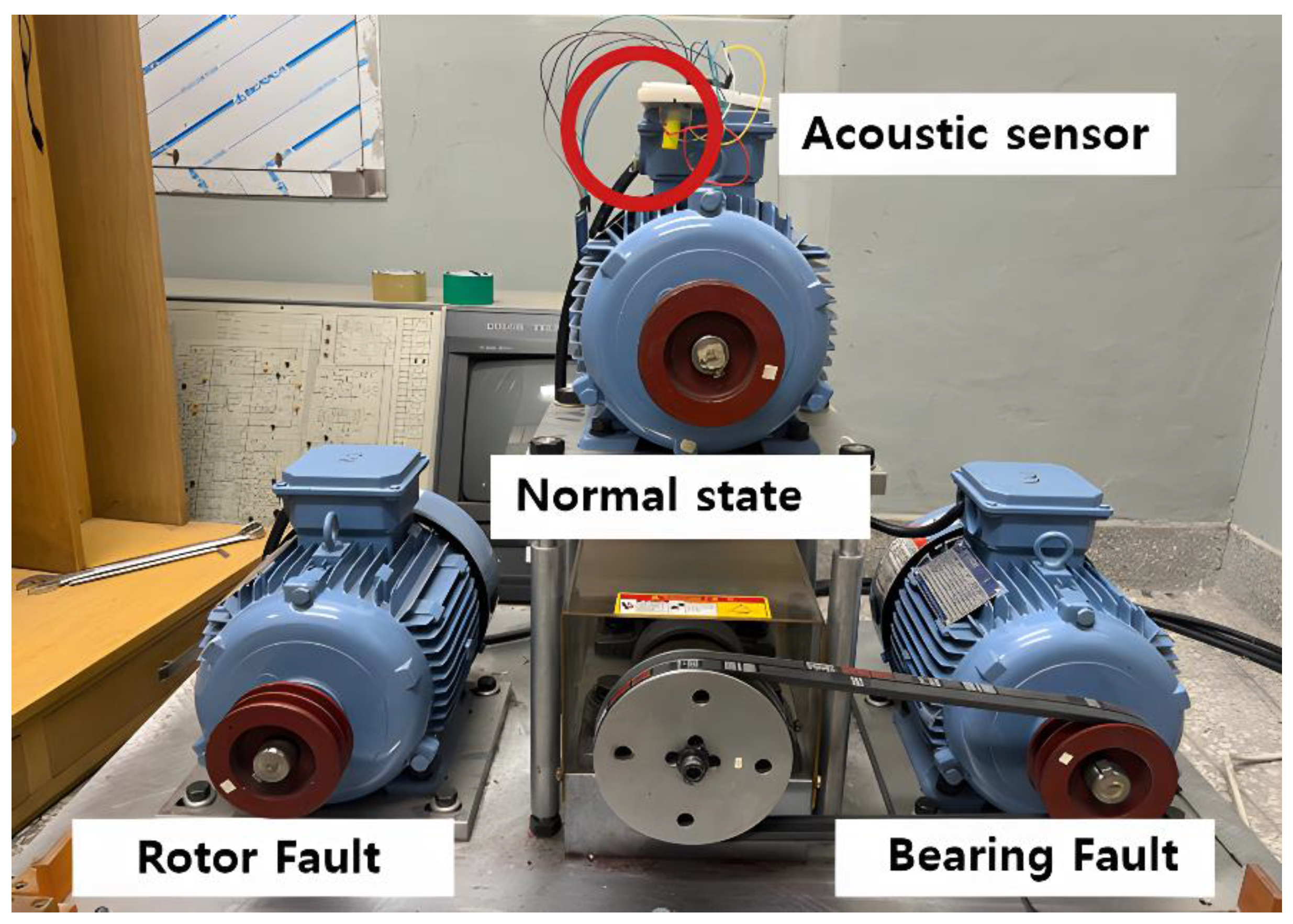
The INMP441 acoustic sensor and a Raspberry Pi were used for data collection. To facilitate mobile data access, the Raspberry Pi was configured as a wireless access point (AP), providing flexibility and convenience during experiments. Figure 7 shows the complete experimental setup. The experiments were carried out in a standard laboratory environment without specialized acoustic chambers. To minimize irregular ambient noise, measurements were taken during quiet periods with minimal external activity. In addition, noise-shielding structures were placed around the microphone to reduce reflections from walls, ceilings, and floors.
A sampling rate of 24 kHz was used, and each recording lasted 15 s. During preprocessing, the initial transient response, defined as the first second of recording, was excluded from the data. The sensor was positioned 15 cm above the motor surface, and the plastic tube used in the shielding structure was 3 cm long. This configuration helped minimize acoustic reflections and ambient noise. A total of 360 samples were collected, with 120 samples per class. All data were acquired under identical environmental conditions and then split into training, validation, and test sets in a 60:20:20 ratio. Preprocessing and subsequent analysis were performed on a PC using the three input representation methods described in Section 1. Figure 8 presents an overview of the experimental rig setup.

3.5. Dataset Construction and Preprocessing Strategy

The acoustic signals from the data acquisition system were used to construct the dataset. For each of the three classes, 120 samples were collected. Each sample had a duration of 14 s after excluding the initial transient response.
In total, 360 samples from all classes were segmented into 1 s intervals, resulting in 5040 samples. These were then divided into 3024 training samples, 1008 validation samples, and 1008 test samples. Z-score normalization was applied across all input data to ensure stable model training by standardizing the scale of the features. Additionally, the physical noise-shielding structure preserved the inherent acoustic signals by reducing noise influence without requiring additional digital filtering.

4. Results

4.1. Time Domain

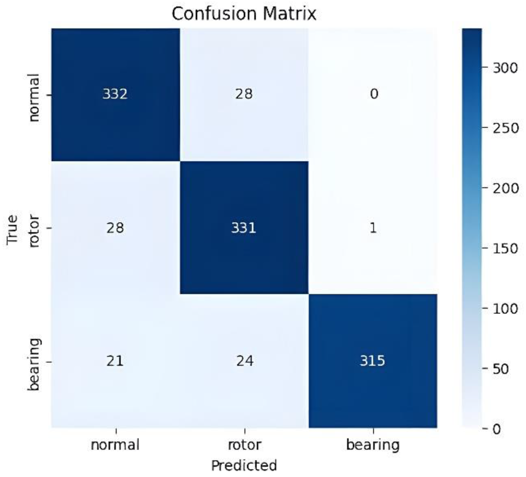
To evaluate the overall performance of the trained model, the confusion matrix for the test set is shown in Figure 9, and the detailed performance metrics are presented in Table 5.
As shown in the confusion matrix (Figure 9), the model made 45 misclassifications in the bearing fault class, and 28 symmetric misclassifications occurred between the normal and rotor fault classes. The model often failed to correctly identify actual bearing faults and had difficulty distinguishing between the normal and rotor conditions. These results highlight the limitations of using time-domain features for fault classification.
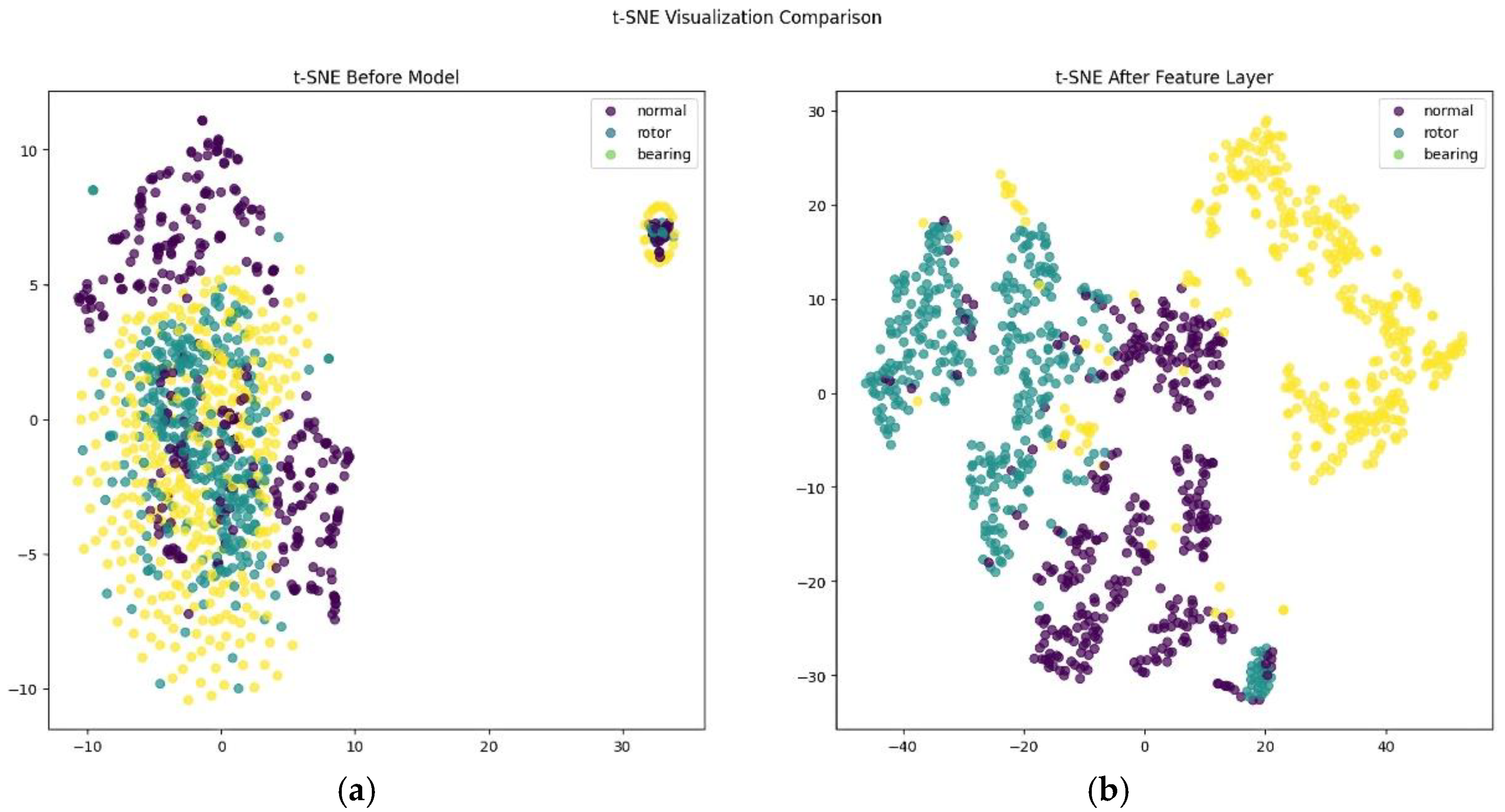
Figure 10 presents a t-SNE visualization of the features learned by the model. t-SNE is a dimensionality reduction technique that projects high-dimensional data into two dimensions, allowing for an intuitive assessment of class separability and data distribution [40]. In Figure 10, the left subplot shows the distribution of raw input data before training, while the right subplot illustrates the feature space after processing through the MNN’s feature extraction layer. Before training, the three classes exhibit substantial overlap, indicating poor class separability. After training, the model learns to form more distinct clusters for each class. However, partial overlap remains between the normal and rotor fault classes, particularly at the boundaries, corroborating the confusion matrix results. Although the bearing class forms a relatively well-defined cluster, some overlap persists, which accounts for its reduced recall. These visualizations confirm that raw time-domain input results in limited class separation.

4.2. Frequency Domain and Statistical Features

As described earlier, frequency-domain signals were divided into 20 equal-frequency bins. From each bin, five statistical features, i.e., mean, variance, median, skewness, and kurtosis, were extracted. Instead of relying on individual features, this multi-dimensional feature vector aimed to improve classification accuracy by capturing diverse signal characteristics. However, under real-world diagnostic conditions the contribution of each feature to classification performance may vary. Therefore, mutual information (MI)-based analysis was conducted to quantitatively assess the influence of each statistical feature on classification. MI is a theoretical measure of dependency between two random variables and is defined in Equation (6) [41]:
I X ; Y K L p x , y p x p y = y Y x X p ( x , y ) log p ( x , y ) p x p ( y )
where X is a feature vector and Y is the class label. p ( x , y ) denotes the joint probability distribution, while p ( x ) and p ( y ) are the marginal distributions of X and Y, respectively. MI is positively associated with the contribution to class separation, indicating that higher values correspond to greater feature contribution.
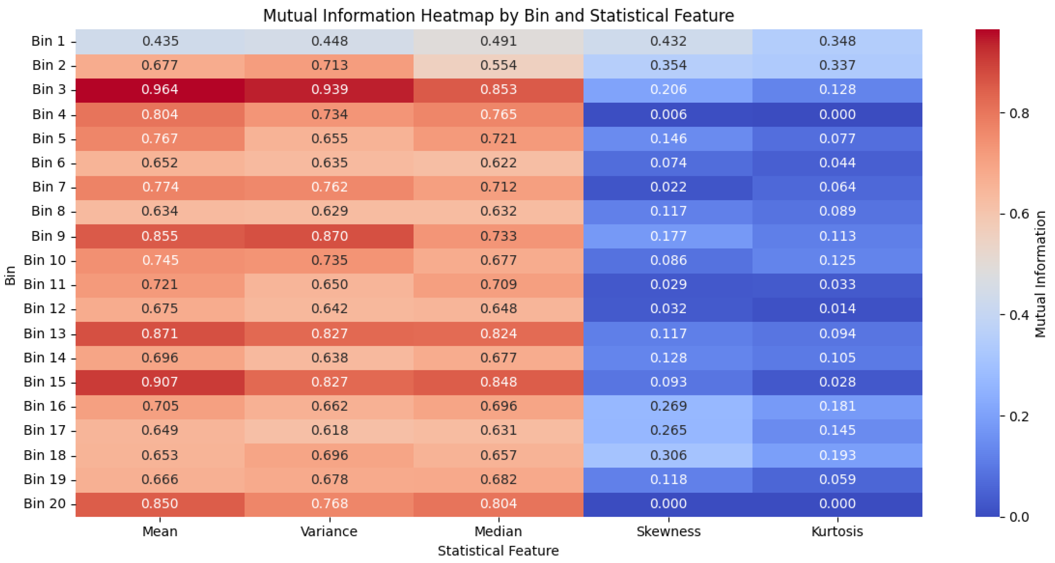
Figure 11 presents a mutual information heatmap of the five statistical features extracted from the 20 frequency bins.
According to the analysis, mean, variance, and median showed consistently high MI values, while skewness and kurtosis contributed significantly less. Notably, the mean, variance, and median in certain bins (e.g., Bins 3, 13, and 15) exceeded MI values of 0.8. In contrast, skewness generally showed MI values below 0.3 across most bins, and kurtosis exhibited even lower values. Morphological features such as skewness and kurtosis approached near-zero MI values in high-frequency bins, indicating limited usefulness for class discrimination.
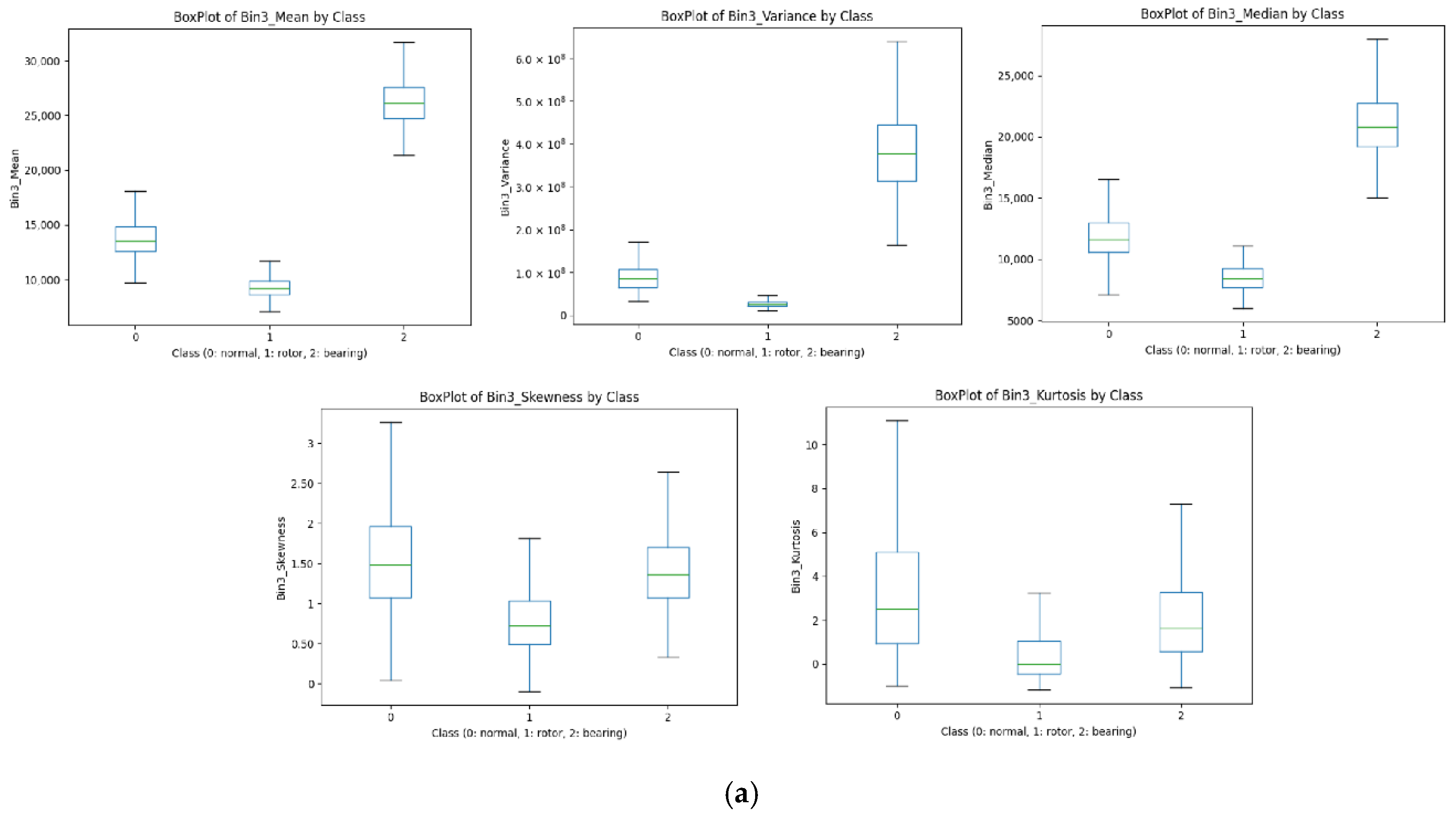
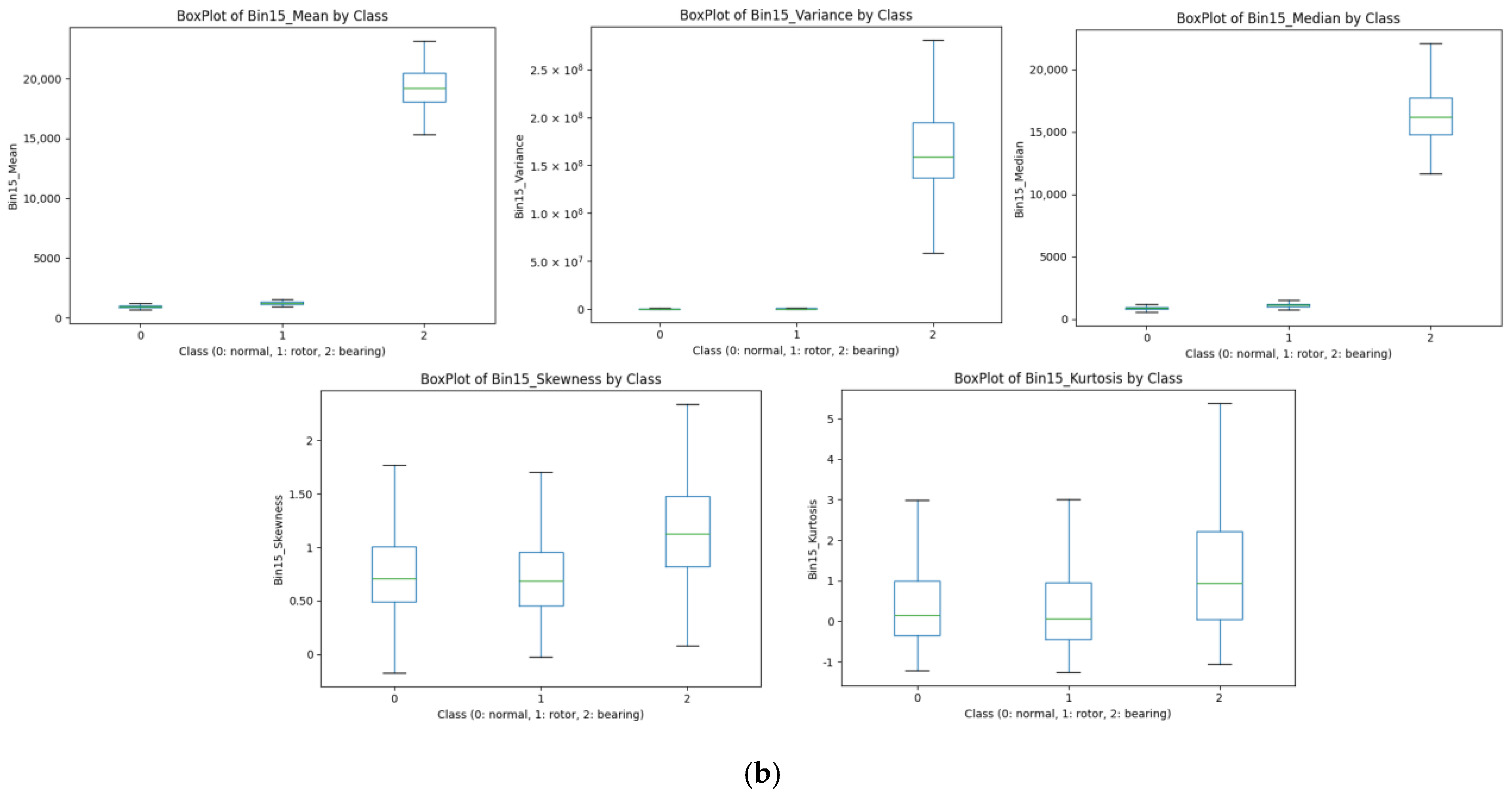
To validate the MI analysis, Figure 12 displays boxplots of class-wise feature distributions for Bins 3 and 15. Each subplot shows the five statistical features—mean, variance, median, skewness, and kurtosis—for the three classes: normal (0), rotor fault (1), and bearing fault (2). The boxplots were generated using the Pandas library in Python 3.
In Figure 12a, the bearing fault class is distinguishable from the others in terms of the mean, while the rotor fault class has the lowest variance. Figure 12b shows even clearer class separation in Bin 15’s mean values: bearing faults produce high values, while the other two classes converge near zero. These patterns reflect the inherent signal characteristics of each fault type. Rotor faults typically produce stable vibrations at specific frequencies, resulting in smaller amplitude fluctuations over time and, consequently, lower variance values. In contrast, bearing faults generate impulsive signals and broadband energy, which increase the mean and median values while also amplifying amplitude variability, leading to higher variance.
In both bins, skewness and kurtosis features show overlapping distributions among classes, reinforcing the MI findings and confirming limited discriminative power.
To further assess the contribution of each feature from a performance perspective, three comparative experiments were conducted using different combinations of statistical features based on the MI and boxplot analyses:
  • Case A: All five features (mean, variance, median, skewness, and kurtosis).
  • Case B: Only high-contribution features (mean, variance, and median).
  • Case C: Only low-contribution features (skewness and kurtosis).
  • Case D: Mixed high- and low-contribution features (mean, variance, median, and skewness).
  • Case E: Mixed high- and low-contribution features (mean, variance, median, and kurtosis).
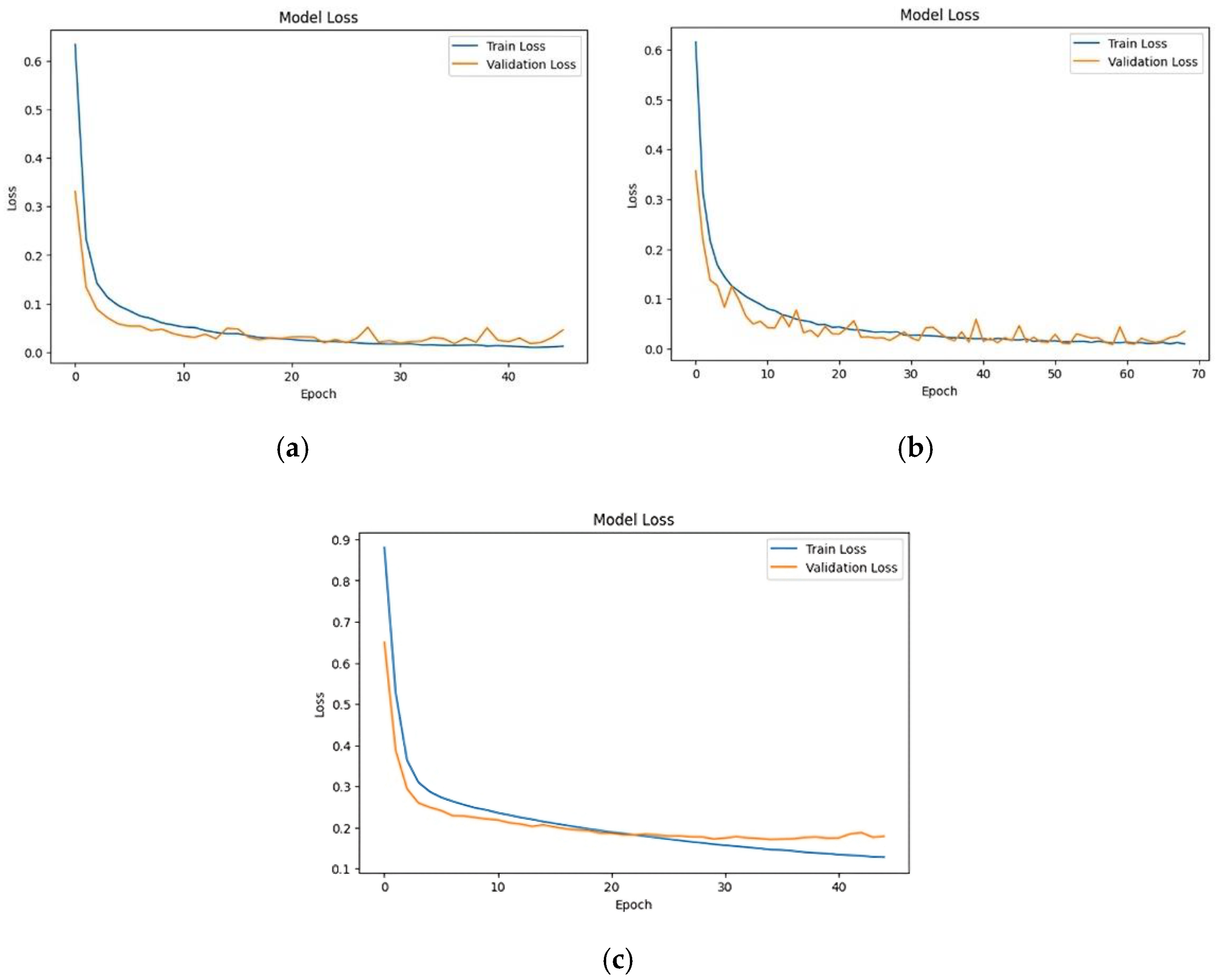
For a fair comparison, the same classification model and hyperparameters were applied to all three cases. During model training, early stopping was used to prevent overfitting. The validation loss was monitored, and training was terminated if no improvement was observed for 10 consecutive epochs. The maximum number of training epochs was set to 500, ensuring that the stopping point was determined by the early stopping criterion. The model weights from the epoch with the lowest validation loss were then restored. Table 6 presents the performance metrics, while Figure 13 and Figure 14 show the respective confusion matrices and loss curves.
Cases A and B achieved similar overall accuracy and F1-scores, but Case B outperformed Case A with a test loss approximately three times lower and a reduction in classification errors from 12 to 2. This result suggests that the inclusion of skewness and kurtosis in Case A may negatively affect the model’s generalization performance. As expected from the MI analysis, Case C—relying solely on skewness and kurtosis—exhibited a substantial drop in performance, with 71 classification errors and the highest test loss. The performance differences between Cases A and D/E were negligible, indicating that the low-MI features contributed little to classification performance for this dataset. While their inclusion did not substantially affect accuracy, it did increase computational load and processing time. Therefore, excluding these features is preferable for efficient model design. These results demonstrate that morphological statistical features alone are inadequate for reliable fault classification.

4.3. Frequency-Domain PCA-Transformed (FFT + PCA)

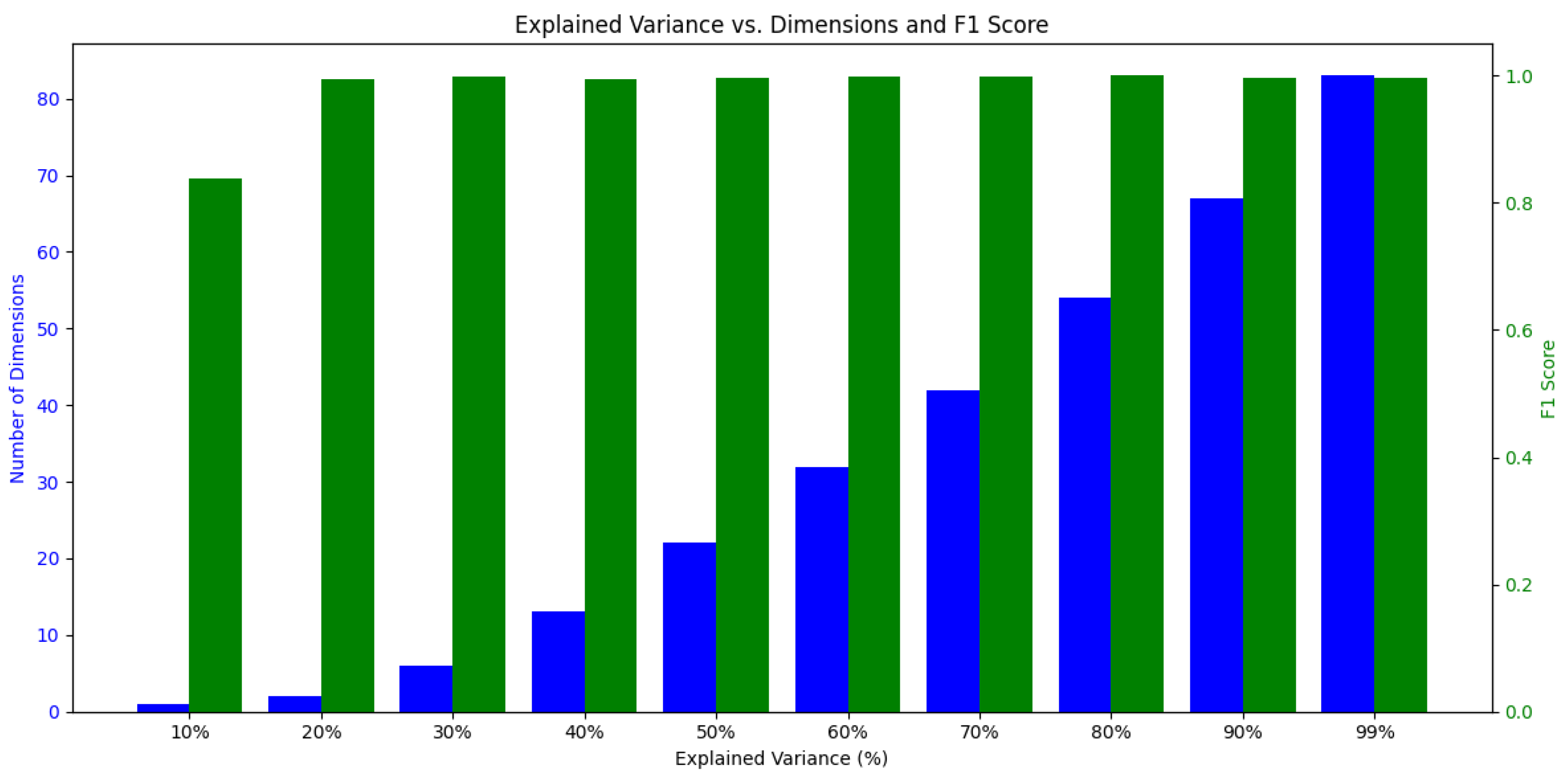
To retain the high classification performance of the FFT + statistical features approach while reducing feature dimensionality, PCA was applied to FFT-transformed data. Figure 15 illustrates how classification performance varies with the explained variance ratio (EVR), ranging from 10% to 99%, helping identify an optimal trade-off between dimensionality reduction and performance retention. High classification accuracy was achieved even at relatively low EVR levels. As EVR increased, the number of required principal components grew substantially, but performance gains remained marginal. Since fault classification accuracy is the primary objective, EVR was selected to strike a balance between optimal performance and reduced dimensionality.
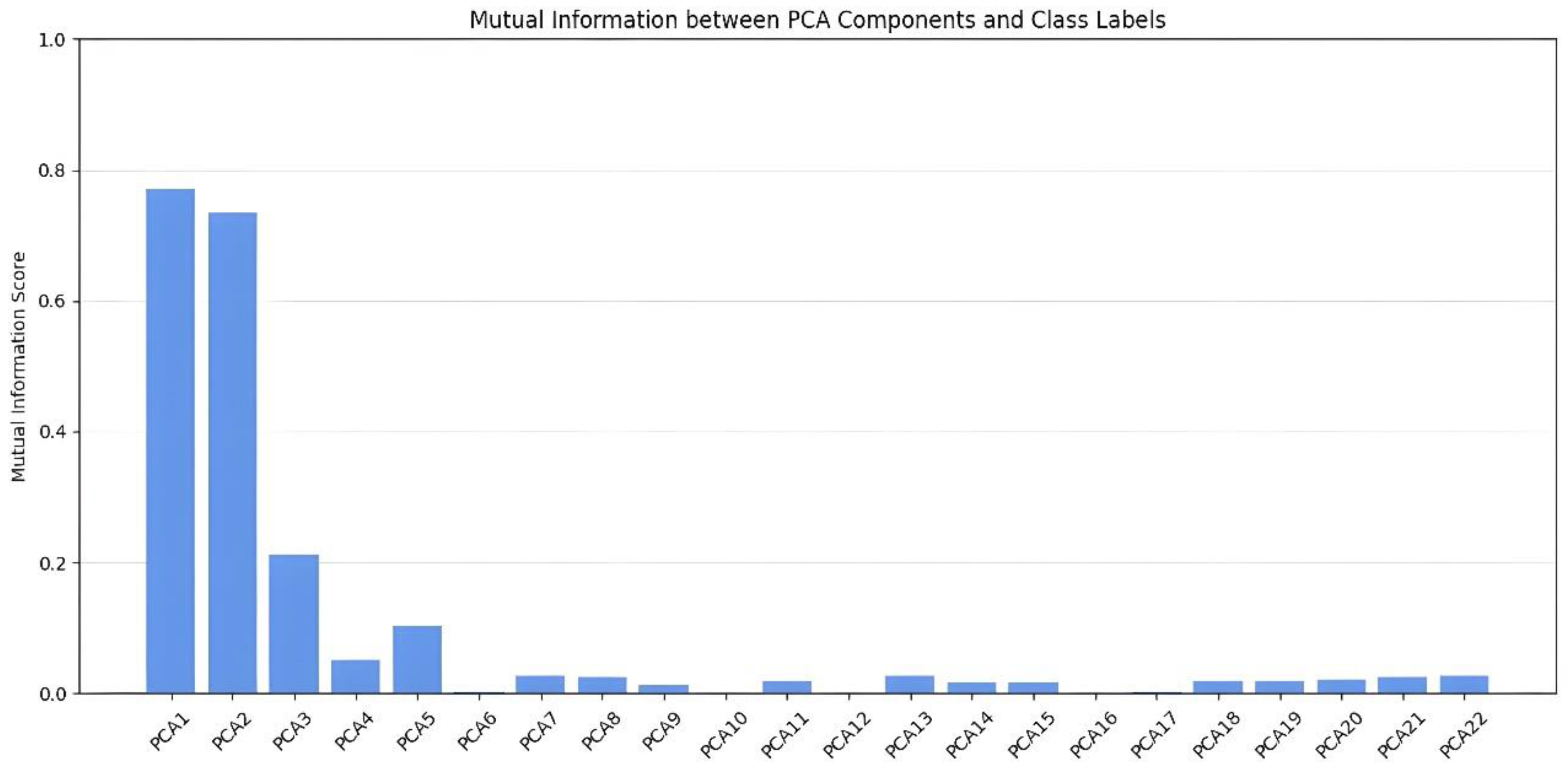
To determine the optimal EVR based on component contribution, the MI between each principal component and the classes was analyzed, as shown in Figure 16.
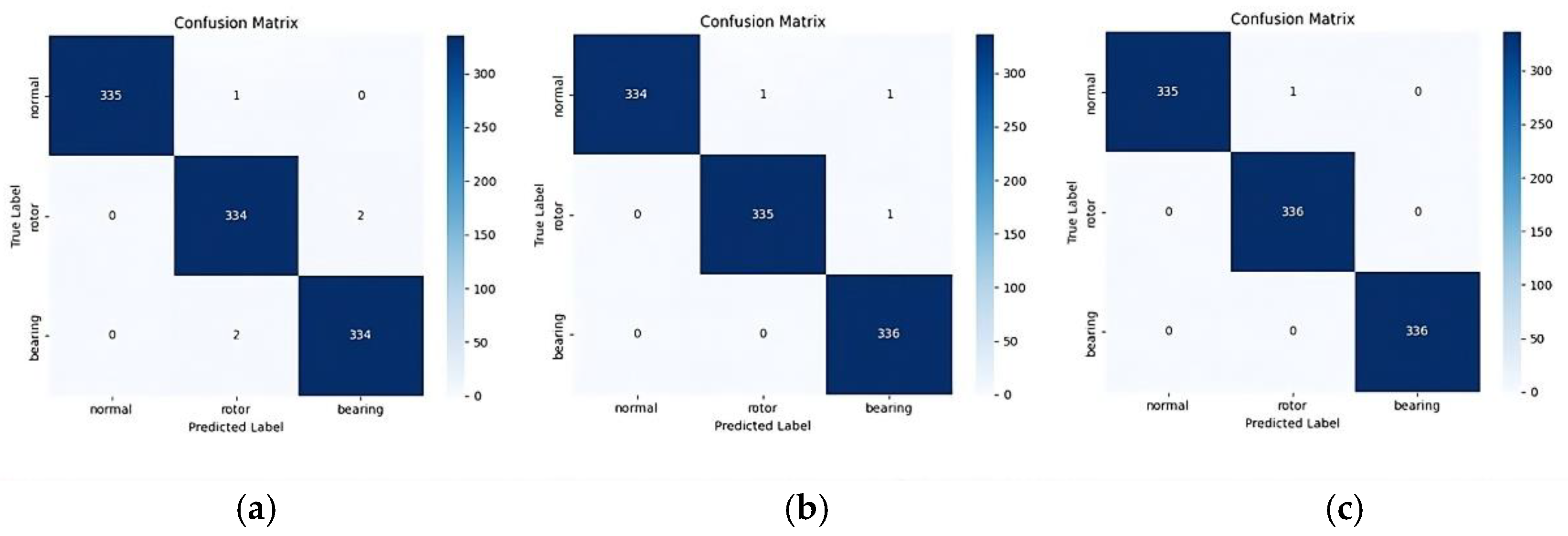
The analysis revealed that PC1 and PC2 were the most influential for class discrimination, with PC3 also showing a moderate contribution. However, a sharp drop in MI was observed for PC4, followed by a slight rebound for PC5. Beyond PC6, the MI values diminished to near-zero, indicating minimal contribution to classification. Based on this analysis, three sets of principal components, PC1-2, PC1-3, and PC1-5, were used in classification experiments. The corresponding confusion matrices are shown in Figure 17.
Although classification performance was generally strong across all configurations, differences in error counts were observed. PC1-2 resulted in five misclassifications, PC1-3 in three, and PC1-5 in only one. While PC1-5 increased feature dimensionality slightly compared to PC1-2, the inclusion of additional components effectively reduced misclassification. As a result, PC1-5 was selected as the optimal configuration. This corresponds to an EVR of 29%, representing a data-driven decision based on both MI analysis and experimental validation. To further assess the robustness of the selected EVR, additional experiments were conducted by varying the EVR threshold to 20%, 40%, 50%, and 70%. Table 7 summarizes the corresponding PCA component counts, F1-scores, and training times. The results clearly indicate that a 29% EVR offers the optimal balance between performance and efficiency for this dataset. At the lower threshold of 20% EVR, classification performance (F1-score) showed a slight decline. In contrast, thresholds above 29% provided no improvement in F1-score but substantially increased model complexity and training time. For instance, at 40% EVR the number of principal components increased by more than 2.5 times (from 5 to 13) compared to 29%, without any performance gain and with a modest increase in training time. Higher thresholds, such as 50% and 70%, further increased both component count and training time, with 70% EVR requiring more than twice the training duration of the 29% configuration. These findings confirm that a 29% EVR provides the most effective trade-off between classification performance, model simplicity, and computational efficiency in the context of this study.
Figure 18 displays the confusion matrix for the final model using PCA-reduced FFT features. Out of 1008 samples, only one normal sample was misclassified as a rotor fault, yielding a classification accuracy of 99.80%. All bearing fault samples were correctly classified.
To further evaluate the separability of PCA-transformed features, t-SNE was used to visualize the five-dimensional feature space, as shown in Figure 19. The visualization reveals distinct clustering for each class: bearing faults (2) formed a compact and isolated cluster in the right region, while the normal (0) and rotor fault (1) classes were well separated in the upper and lower regions, respectively. These results demonstrate that the five-dimensional PCA features offer strong discriminative power, supporting the 99.80% classification accuracy.

4.4. Discussion of Results

The performance summary of the three methods is presented in Table 8. The raw time-domain signal method achieved an accuracy of 90.6%, but it showed clear limitations, including frequent misclassifications between normal and rotor fault conditions and a low recall rate for bearing faults. The FFT combined with statistical feature extraction improved performance, as mutual information analysis identified the mean, variance, and median as more informative features than skewness and kurtosis. Using only the high-contribution statistical features, this method reached 99.8% accuracy, with just two misclassifications. The FFT + PCA approach outperformed all other methods, achieving the highest classification accuracy of 99.9% while significantly reducing input dimensionality. By selecting a 29% explained variance ratio based on performance criteria, the method reduced feature dimensions from 60 to 5, maintaining excellent diagnostic performance with only one misclassification.
The raw time-domain input with 24,000 nodes required approximately 384,000 parameters in the first fully connected layer alone. In contrast, the FFT + statistical features (Case A), with only 100 nodes, required about 1600 parameters, a roughly 238-fold reduction. This reduction proportionally decreased the number of multiply–accumulate operations, resulting in a substantial decrease in both computational cost and memory usage. Beyond improving training efficiency, this dimensionality reduction also helped mitigate the risk of overfitting associated with high-dimensional inputs. An alternative approach for directly processing raw time-domain signals, while reducing computational load and effectively capturing local features, is the use of 1D-CNNs.
To quantitatively validate the practicality of using low-cost sensors and lightweight models, Table 9 compares key deployment-related metrics—parameter count, MACs per sample, and average inference time—across different feature extraction methods. The inference times reported here represent pure forward-pass latency (excluding preprocessing) and were measured with a batch size of 1 under identical hardware conditions. All three input methods achieved inference times of approximately 0.6 ms, confirming their suitability for real-time diagnosis. However, despite the substantial reduction in parameter count and MAC operations, inference times remained similar because fixed overheads, such as framework calls, memory access, and data loading, dominated the overall latency. This is a well-known characteristic of lightweight models, where differences in computational complexity are not directly reflected in inference time.
From a computational standpoint, the FFT + PCA method achieved a dramatic 99.93% reduction in both parameter count (384,179 → 259) and MACs (384,152 → 232). This highlights its advantage in reducing model size and computational demand while maintaining real-time diagnostic capability, as demonstrated by the inference time results.

5. Conclusions

This study conducted a comparative analysis of three input representation methods for induction motor fault diagnosis using a low-cost acoustic sensor and a lightweight MNN architecture: time-domain raw waveforms, FFT-based statistical features, and FFT-based PCA features. Among these, the time-domain approach achieved the lowest accuracy (90.6%), the FFT method with high-contribution statistical features reached 99.8%, and the FFT + PCA method achieved the highest accuracy (99.9%) while reducing feature dimensions from 60 to 5. All three methods recorded inference times of approximately 0.6 ms, confirming their suitability for real-time diagnosis. The FFT + PCA approach also reduced the parameter count and MACs by 99.93%, underscoring its advantage in minimizing model size and computational demand without compromising diagnostic performance.
This extreme model compression demonstrates the practicality of the proposed method and validates its feasibility for deployment in real-world field environments. The findings confirm that high-accuracy fault diagnosis can be achieved without complex signal processing or high-performance computing resources, supporting the industrial applicability of low-cost, sensor-based systems.
This study’s limitations include reliance on a single induction motor dataset, a limited variety of fault types, and the absence of varying load conditions, which likely simplified the classification task compared to real-world scenarios. To address these limitations and ensure robustness in practical applications, future work will validate the proposed approach in more realistic industrial environments that include noise, varying loads, and diverse motor types and specifications. Additional research will explore the use of 1D-CNNs for enhanced feature extraction and reduced overfitting. Furthermore, the FFT + PCA framework could be adapted for real-time diagnosis on embedded devices, enabling immediate fault detection and integration with alarm systems. Finally, incorporating dynamic feature selection through online learning may further improve adaptability by updating the optimal feature set in response to changing load and operating conditions.

Author Contributions

Conceptualization, S.M.Y. and I.S.L.; methodology, S.M.Y. and I.S.L.; investigation, S.M.Y., H.G.L. and W.K.H.; experiments, S.M.Y., H.G.L. and W.K.H.; simulations, S.M.Y.; data analysis, S.M.Y. and I.S.L.; writing—original draft, S.M.Y.; writing—review & editing, S.M.Y. and I.S.L.; supervision, I.S.L. All authors have read and agreed to the published version of the manuscript.

Funding

This research was funded by the Ministry of Education (Korea) under the BK21 FOUR project, grant number 4199990113966.

Institutional Review Board Statement

Not applicable.

Informed Consent Statement

Not applicable.

Data Availability Statement

The data presented in this study are available from the corresponding author upon reasonable request.

Conflicts of Interest

The authors declare no conflicts of interest.

Nomenclature

CCovariance matrix representing the linear correlation between variables
I(X; Y)Mutual information between X and Y
NTotal number of samples
TNumber of samples per second
WnWeight matrix of the n-th hidden layer
Xkk-th frequency component of the input signal (complex value)
bnBias vector of the n-th hidden layer
n(t)Environmental noise component
s(t)Actual signal generated by the induction motor
t_iTime corresponding to the i-th sample
vii-th eigenvector
xInput feature vector
x_iAmplitude value if the i-th sample
x(t)Signal amplitude at time t (raw time-domain signal)
xnn-th sample value of the input signal in time domain
λiEigenvalue corresponding to the i-th eigenvector

References

  1. Cao, W.; Mecrow, B.C.; Atkinson, G.J.; Bennett, J.W.; Atkinson, D.J. Overview of Electric Motor Technologies Used for More Electric Aircraft (MEA). IEEE Trans. Ind. Electron. 2012, 59, 3523–3531. [Google Scholar] [CrossRef]
  2. Jigyasu, R.; Sharma, A.; Mathew, L.; Chatterji, S. A Review of Condition Monitoring and Fault Diagnosis Methods for Induction Motor. In Proceedings of the Second International Conference on Intelligent Computing and Control Systems (ICICCS 2018), Madurai, India, 14–15 June 2018; pp. 1713–1721. [Google Scholar] [CrossRef]
  3. Xu, Z.; Tang, G.; Pang, B. An Infrared Thermal Image Few-Shot Learning Method Based on CAPNet and Its Application to Induction Motor Fault Diagnosis. IEEE Sens. J. 2022, 22, 16440–16450. [Google Scholar] [CrossRef]
  4. Abdelmaksoud, M.; Torki, M.; El-Habrouk, M.; Elgeneidy, M. Convolutional-Neural-Network-Based Multi-Signals Fault Diagnosis of Induction Motor Using Single and Multi-Channels Datasets. Alex. Eng. J. 2023, 73, 231–248. [Google Scholar] [CrossRef]
  5. Sheikh, M.A.; Bakhsh, S.T.; Irfan, M.; Nor, N.b.M.; Nowakowski, G. A Review to Diagnose Faults Related to Three-Phase Industrial Induction Motors. J. Fail. Anal. Prev. 2022, 22, 1546–1557. [Google Scholar] [CrossRef]
  6. Choi, S.; Pazouki, E.; Baek, J.; Bahrami, H.R. Iterative Condition Monitoring and Fault Diagnosis Scheme of Electric Motor for Harsh Industrial Application. IEEE Trans. Ind. Electron. 2015, 62, 1760–1769. [Google Scholar] [CrossRef]
  7. Supriyono, J.; Mukhlash, I.; Iqbal, M.; Asfani, D.A. Early Warning Forecasting of Large Induction Motor in the Oil and Gas Industry from Deep Learning. In Proceedings of the 2024 IEEE International Symposium on Consumer Technology (ISCT), Kuta, Indonesia, 22–24 January 2024; pp. 436–442. [Google Scholar] [CrossRef]
  8. Ramana, D.V.; Baskar, S. Diverse Fault Detection Techniques of Three-Phase Induction Motor—A Review. In Proceedings of the 2016 International Conference on Emerging Technological Trends (ICETT), Kollam, India, 21–23 October 2016; pp. 1–8. [Google Scholar] [CrossRef]
  9. Jorkesh, S.; Poshtan, J. Fault Diagnosis of an Induction Motor Using Data Fusion Based on Neural Networks. IET Sci. Meas. Technol. 2021, 15, 681–689. [Google Scholar] [CrossRef]
  10. Bahgat, B.H.; Elhay, E.A.; Elkholy, M.M. Advanced Fault Detection Technique of Three Phase Induction Motor: Comprehensive Review. Discov. Electron. 2024, 1, 9. [Google Scholar] [CrossRef]
  11. Mehrjou, M.R.; Mariun, N.; Marhaban, M.H.; Misron, N. Rotor Fault Condition Monitoring Techniques for Squirrel-Cage Induction Machine—A Review. Mech. Syst. Signal Process. 2011, 25, 2827–2848. [Google Scholar] [CrossRef]
  12. Allal, A.; Khechekhouche, A. Diagnosis of Induction Motor Faults Using the Motor Current Normalized Residual Harmonic Analysis Method. Int. J. Electr. Power Energy Syst. 2022, 141, 108219. [Google Scholar] [CrossRef]
  13. Zarei, J. Induction Motors Bearing Fault Detection Using Pattern Recognition Techniques. Expert Syst. Appl. 2012, 39, 68–73. [Google Scholar] [CrossRef]
  14. Glowacz, A.; Glowacz, Z. Diagnosis of Stator Faults of the Single-Phase Induction Motor Using Acoustic Signals. Appl. Acoust. 2017, 117, 20–27. [Google Scholar] [CrossRef]
  15. Bazurto, A.J.; Quispe, E.C.; Mendoza, R.C. Causes and Failures Classification of Industrial Electric Motor. In Proceedings of the 2016 IEEE ANDESCON, Arequipa, Peru, 19–21 October 2016; pp. 1–4. [Google Scholar] [CrossRef]
  16. Ewert, P. Use of Axial Flux in the Detection of Electrical Faults in Induction Motors. In Proceedings of the 2017 International Symposium on Electrical Machines (ISEM), Naleczow, Poland, 5–8 September 2017; pp. 1–6. [Google Scholar] [CrossRef]
  17. Khechekhouche, A.; Cherif, H.; Benakcha, A.; Menacer, A.; Chehaidia, S.E.; Panchal, H. Experimental Diagnosis of Inter-Turns Stator Fault and Unbalanced Voltage Supply in Induction Motor Using MCSA and DWER. Period. Eng. Nat. Sci. 2020, 8, 1202–1216. [Google Scholar]
  18. Benamira, N.; Dekhane, A.; Bouraiou, A.; Atoui, I. Exploring the Effects of Overvoltage Unbalances on Three Phase Induction Motors: Insights from Motor Current Spectral Analysis and Discrete Wavelet Transform Energy Assessment. Comput. Electr. Eng. 2024, 117, 109242. [Google Scholar] [CrossRef]
  19. Martínez-Morales, J.D.; Palacios-Hernández, E.R.; Campos-Delgado, D.U. Multiple-Fault Diagnosis in Induction Motors through Support Vector Machine Classification at Variable Operating Conditions. Electr. Eng. 2018, 100, 59–73. [Google Scholar] [CrossRef]
  20. Ballal, M.S.; Khan, Z.J.; Suryawanshi, H.M.; Sonolikar, R.L. Induction Motor: Fuzzy System for the Detection of Winding Insulation Condition and Bearing Wear. Electr. Power Compon. Syst. 2006, 34, 159–171. [Google Scholar] [CrossRef]
  21. Halder, S.; Bhat, S.; Zychma, D.; Sowa, P. Broken Rotor Bar Fault Diagnosis Techniques Based on Motor Current Signature Analysis for Induction Motor—A Review. Energies 2022, 15, 8569. [Google Scholar] [CrossRef]
  22. Yakhni, M.F.; Cauet, S.; Sakout, A.; Assoum, H.; Etien, E.; Rambault, L.; El-Gohary, M. Variable Speed Induction Motors’ Fault Detection Based on Transient Motor Current Signatures Analysis: A Review. Mech. Syst. Signal Process. 2023, 184, 109737. [Google Scholar] [CrossRef]
  23. Zhu, Q.; Zhu, L.; Wang, Z.; Zhang, X.; Li, Q.; Han, Q.; Yang, Z.; Qin, Z. Hybrid Triboelectric-Piezoelectric Nanogenerator Assisted Intelligent Condition Monitoring for Aero-Engine Pipeline System. Chem. Eng. J. 2025, 519, 165121. [Google Scholar] [CrossRef]
  24. Cao, J.; Lin, Y.; Fu, X.; Wang, Z.; Liu, G.; Zhang, Z.; Qin, Y.; Zhou, H.; Dong, S.; Cheng, G.; et al. Self-Powered Overspeed Wake-Up Alarm System Based on Triboelectric Nanogenerators for Intelligent Transportation. Nano Energy 2023, 107, 108150. [Google Scholar] [CrossRef]
  25. Tang, S.; Khoo, B.C.; Zhu, Y.; Lim, K.M.; Yuan, S. A Light Deep Adaptive Framework toward Fault Diagnosis of a Hydraulic Piston Pump. Appl. Acoust. 2024, 217, 109807. [Google Scholar] [CrossRef]
  26. Zhou, L.; Zhao, Q.; Zeng, J.; Zhu, A.; Long, X.; He, L. Fault Diagnosis and Data Reconstruction of Temperature Sensors for Wind Turbine Stator Winding. Shock Vib. 2025, 2025, 4713545. [Google Scholar] [CrossRef]
  27. Han, C.; Liu, T.; Wang, Y.; Li, X.; Kou, Z.; Yang, G. Multi-Sensor Adaptive Fusion and Convolutional Neural Network-Based Acoustic Emission Diagnosis for Initial Damage of the Engine. Meas. Sci. Technol. 2025, 36, 026133. [Google Scholar] [CrossRef]
  28. Toma, R.N.; Prosvirin, A.E.; Kim, J.-M. Bearing Fault Diagnosis of Induction Motors Using a Genetic Algorithm and Machine Learning Classifiers. Sensors 2020, 20, 1884. [Google Scholar] [CrossRef]
  29. Tran, M.-Q.; Liu, M.-K.; Tran, Q.-V.; Nguyen, T.-K. Effective Fault Diagnosis Based on Wavelet and Convolutional Attention Neural Network for Induction Motors. IEEE Trans. Instrum. Meas. 2022, 71, 3501613. [Google Scholar] [CrossRef]
  30. You, K.; Qiu, G.; Gu, Y. Rolling Bearing Fault Diagnosis Using Hybrid Neural Network with Principal Component Analysis. Sensors 2022, 22, 8906. [Google Scholar] [CrossRef]
  31. Choudhary, A.; Goyal, D.; Letha, S.S. Infrared Thermography-Based Fault Diagnosis of Induction Motor Bearings Using Machine Learning. IEEE Sens. J. 2021, 21, 1727–1734. [Google Scholar] [CrossRef]
  32. Germen, E.; Başaran, M.; Fidan, M. Sound Based Induction Motor Fault Diagnosis Using Kohonen Self-Organizing Map. Mech. Syst. Signal Process. 2014, 46, 45–58. [Google Scholar] [CrossRef]
  33. Nandi, S.; Toliyat, H.A.; Li, X. Condition Monitoring and Fault Diagnosis of Electrical Motors—A Review. IEEE Trans. Energy Convers. 2005, 20, 719–729. [Google Scholar] [CrossRef]
  34. Nussbaumer, H.J. The Fast Fourier Transform. In Fast Fourier Transform and Convolution Algorithms; Springer Series in Information Sciences; Springer: Berlin/Heidelberg, Germany, 1982; Volume 2, pp. 80–111. [Google Scholar] [CrossRef]
  35. Rousseeuw, P.J.; Hubert, M. Robust Statistics for Outlier Detection. WIREs Data Min. Knowl. Discov. 2011, 1, 73–79. [Google Scholar] [CrossRef]
  36. Doane, D.P.; Seward, L.E. Measuring Skewness: A Forgotten Statistic? J. Stat. Educ. 2011, 19, 1–18. [Google Scholar] [CrossRef]
  37. Westfall, P.H. Kurtosis as Peakedness, 1905–2014. R.I.P. Am. Stat. 2014, 68, 191–195. [Google Scholar] [CrossRef] [PubMed]
  38. Brys, G.; Hubert, M.; Struyf, A. A Robust Measure of Skewness. J. Comput. Graph. Stat. 2004, 13, 996–1017. [Google Scholar] [CrossRef]
  39. Abdi, H.; Williams, L.J. Principal Component Analysis. WIREs Comput. Stat. 2010, 2, 433–459. [Google Scholar] [CrossRef]
  40. van der Maaten, L.; Hinton, G. Visualizing Data Using t-SNE. J. Mach. Learn. Res. 2008, 9, 2579–2605. [Google Scholar]
  41. Kraskov, A.; Stögbauer, H.; Grassberger, P. Estimating Mutual Information. Phys. Rev. E 2004, 69, 066138. [Google Scholar] [CrossRef]
Figure 1. Acquired waveform data of the induction motor over a 0.1 s interval: (a) Normal condition; (b) Rotor fault; and (c) Bearing fault.
Applsci 15 09379 g001
Figure 2. Frequency-domain spectra of the three motor states: (a) Normal; (b) Rotor fault; and (c) Bearing fault.
Applsci 15 09379 g002
Figure 3. Overall experimental flowchart.
Applsci 15 09379 g003
Figure 4. Fault types: (a) Bearing fault with iron powder contamination; (b) Rotor fault with drilled rotor bar.
Applsci 15 09379 g004aApplsci 15 09379 g004b
Figure 5. Plastic tube-based shielding structure for the INMP441 sensor, highlighted by the red circle in the experimental setup.
Applsci 15 09379 g005
Figure 6. Frequency spectra comparison before and after shielding implementation.
Applsci 15 09379 g006
Figure 7. Experimental setup and sensor placement, with the red circle highlighting the acoustic sensor mounted in the motor housing.
Applsci 15 09379 g007
Figure 8. Overview of the experimental rig setup.
Applsci 15 09379 g008
Figure 9. Confusion matrix for time-domain classification.
Applsci 15 09379 g009
Figure 10. t-SNE visualization before and after MNN training: (a) raw input data before training; (b) feature representation after the MNN’s feature extraction layer.
Applsci 15 09379 g010
Figure 11. Mutual information heatmap of statistical features across frequency bins.
Applsci 15 09379 g011
Figure 12. Boxplots of feature distributions by class: (a) Bin 3 and (b) Bin 15.
Applsci 15 09379 g012aApplsci 15 09379 g012b
Figure 13. Confusion matrices for different statistical feature combinations: (a) Case A (all five statistical features); (b) Case B (high-contribution features); and (c) Case C (low-contribution features).
Applsci 15 09379 g013
Figure 14. Training and validation loss curves for different feature combinations: (a) Case A (all five statistical features); (b) Case B (high-contribution features); and (c) Case C (low-contribution features).
Applsci 15 09379 g014
Figure 15. Changes in dimensionality (blue) and F1-score (green) with respect to EVR.
Applsci 15 09379 g015
Figure 16. Mutual information analysis between principal components and class labels.
Applsci 15 09379 g016
Figure 17. Confusion matrices for different PCA configurations: (a) PC1-2; (b) PC1-3; and (c) PC1-5.
Applsci 15 09379 g017
Figure 18. Confusion matrix for MNN classifier with PCA-reduced features.
Applsci 15 09379 g018
Figure 19. t-SNE visualization of the feature space after PCA-based dimensionality reduction.
Applsci 15 09379 g019
Table 1. Formulas of statistical features.
Statistical FeaturesEquation
Mean μ = 1 N i = 1 N x i
Variance σ 2 = 1 N i = 1 N ( x i μ ) 2
Median x ( n + 1 ) / 2       i f   n   i s   o d d 1 2 x n 2 + x n 2 + 1   i f   n   i s   e v e n
Skewness 1 N i = 1 N x i μ σ 3
Kurtosis 1 N i = 1 N x i μ σ 4
Table 2. Detailed network structure and hyperparameters in this experiment.
ParameterValue
Network ArchitectureHidden Layer 116 nodes
Hidden Layer 28 nodes
Hidden Layer 33 nodes
Activation FunctionsHidden LayersReLU
Output LayerSoftmax
Training ParametersOptimizerAdam
Learning Rate0.001
Batch Size32
Classification ClassesClass 0Normal
Class 1Rotor Fault
Class 2Bearing Fault
Table 3. Specifications of the induction motor.
ParameterValueParameterValue
Rated Power2.2 kWNumber of poles4
Rated voltage220/380 VRated frequency60 Hz
Rated speed1730 rpmDirectivityOmnidirectional
Protection ClassIP54Efficiency82.0%
Table 4. Specification of the INMP441 microphone.
ParameterValueParameterValue
Sensitivity−26 dBFSMax SPL120 dB SPL
Signal-to-Noise Ratio60 dBAOutput FormatI2S
Frequency Response10 Hz–10 kHzDirectivityOmnidirectional
Table 5. Performance metrics for time-domain input.
ClassPrecisionRecallF1-Score
Normal0.8710.9220.896
Rotor0.8650.9190.891
Bearing0.9970.8750.932
Table 6. Classification performance for different statistical feature combinations.
Title 1Case ACase BCase CCase DCase E
Test Loss0.03300.01010.18200.03800.0328
Error count122711212
Accuracy0.98810.99800.92940.98910.9881
Precision0.98800.99800.92940.98850.9883
Recall0.98810.99800.92960.98810.9880
F1-score0.98790.99800.92940.98810.9881
Epochs3453465339
Table 7. Effect of EVR thresholds on PCA components, classification performance, and training time.
EVR (%)PCA ComponentsF1-ScoreTraining Time (s)
2020.993113
2950.998015
40130.998017
50220.998029
70420.998031
Table 8. Classification performance comparison by feature extraction method.
MethodInput Feature# of Input NodesAccuracyF1-Score# of Errors
Time domainRaw signal24,00090.6%0.907101
FFT + Statistical featuresAll features
(Case A)
10098.8%0.98812
High-contribution (Case B)6099.8%0.9982
Low-contribution (Case C)4092.4%0.92471
FFT + PCA29% EVR599.9%0.9991
Table 9. Comparison of parameters, MACs/sample, and inference time (batch = 1, excluding preprocessing) by feature extraction method.
MethodInput FeatureParametersMACs/SampleAvg.
Inference Time
(ms, Batch Size = 1)
Time domainRaw signal384,179384,1520.613
FFT + Statistical featuresHigh-contribution (Case B)113911120.589
FFT + PCA29% EVR2592320.585
Disclaimer/Publisher’s Note: The statements, opinions and data contained in all publications are solely those of the individual author(s) and contributor(s) and not of MDPI and/or the editor(s). MDPI and/or the editor(s) disclaim responsibility for any injury to people or property resulting from any ideas, methods, instructions or products referred to in the content.