Abstract
In underground coal mines, narrow and irregular tunnels, dust, and gas hazards pose significant challenges to robotic path planning, particularly for shotcrete operations. The traditional A* algorithm has the limitations of limited safety, excessive node expansion, and insufficient dynamic obstacle avoidance capabilities. To address these, a hybrid algorithm integrating adaptive A*, Q-learning, and the Dynamic Window Approach (DWA) is proposed. The A* component is enhanced through improvements to its evaluation function and node selection strategy, incorporating dynamically adjustable neighborhood sampling to improve search efficiency. Q-learning re-plans unsafe trajectories in complex environments using a redesigned reward mechanism and an adaptive exploration strategy. The DWA module facilitates real-time obstacle avoidance in dynamic scenarios by optimizing both the velocity space and the trajectory evaluation process. The simulation results indicate that the proposed algorithm reduces the number of path nodes by approximately 30%, reduces the computational time by approximately 20% on 200 × 200 grids, and increases the path length by only 10%. These results demonstrate that the proposed approach effectively balances global path optimality with local adaptability, significantly improving the safety and real-time performance in complex underground environments.
1. Introduction
1.1. Background
As a foundational energy source and essential raw material, coal necessitates environmentally sustainable mining practices and rational utilization. In underground coal mining, shotcrete robots are employed to perform tunnel support spraying. These robots require robust global path planning to navigate safely through narrow, obstacle-dense tunnels. However, their operational efficiency is often limited by the complexity of underground environments [1,2]. With the continued advancement of intelligent transformation in China’s coal industry, achieving the autonomous operation of shotcrete robots has emerged as a promising solution. SLAM-based (Simultaneous Localization and Mapping) path planning is critical for designing motion trajectories of shotcrete robots operating in complex environments. This study aims to develop advanced algorithms for planning safe and efficient paths for shotcrete robots in underground coal tunnels, with adaptability to dynamic and unpredictable conditions to ensure reliable and effective shotcrete operations.
1.2. Related Work
Path planning methodologies are typically classified into global and local approaches. Global planners, such as Rapidly exploring Random Trees (RRT) [3,4,5] and A* algorithms [6,7,8], operate based on prior environmental maps and are well suited for structured, static environments. In contrast, local planning strategies—such as the DWA [9] and the Artificial Potential Field (APF) method [10]—leverage real-time sensor data to navigate around unknown or dynamic obstacles without requiring complete environmental information.
Among the existing algorithms, the A* algorithm efficiently identifies optimal paths in static environments through a heuristic-guided node expansion strategy, and its performance advantages have been extensively validated in robotics applications.
However, despite its theoretical optimality under the admissible heuristic condition [6], the traditional A* algorithm demonstrates notable limitations in complex environments. Its reliance on fixed eight-neighborhood search and a Euclidean distance heuristic (Equation (2)) leads to suboptimal node expansion in several respects: (1) the uniform sampling strategy results in approximately 30% redundant nodes in 200 × 200 grids due to the unnecessary exploration of regions adjacent to obstacles; (2) the absence of geometric constraints on turning angles causes abrupt path deviations exceeding 90°, violating robot kinematic constraints; (3) the heuristic function disregards safety distance metrics, resulting in 65% of nodes lying within one grid unit of obstacles, thereby violating the Markov property required for safe navigation [11].
In optimizing the A* algorithm for path planning, Table 1 organizes research findings by algorithm type, core improvements, and limitations, presenting the research status and guiding future enhancements.

Table 1.
A*-based algorithm variants: improvements and limitations.
Table 1.
A*-based algorithm variants: improvements and limitations.
| Author | Algorithm Type | Core Improvements | Existing Limitations |
|---|---|---|---|
| Zhang et al. [12] | Hybrid Algorithm (Improved A* + DWA) | 1. Improved A*: Optimizes path efficiency and smoothness through adjustment factors, 5-neighborhood search, and Floyd’s algorithm. 2. Improved DWA: Introduces a smoothing coefficient and a local target selection strategy. | 1. A* has fixed neighborhood sampling (only 5-neighborhood), which cannot adapt to changes in obstacle distribution. 2. No safety distance constraint is set, so the path is prone to being close to obstacles. |
| Fu et al. [13] | Adaptive A* | 1. Optimizes traditional neighborhood to 16-neighborhood. 2. Removes redundant path points via node deletion, bidirectional search, and dynamic weights. | 1. 16-neighborhood expands search space exponentially, increasing computation time. 2. Unoptimized turning angle may violate robot kinematic constraints. |
| Jin et al. [14] | Adaptive A* | Reduces node redundancy and improves search efficiency via 5-neighborhood filtering. | 1. Failure to address turning angle optimization; path may have sharp turns (>90°). 2. No dynamic obstacle avoidance capability. |
These studies collectively underscore a critical gap: the need for dynamic search strategies that balance path safety, smoothness, and computational efficiency in complex environments. Different from the above studies, this algorithm achieves a 30% reduction in the number of nodes, controls the average turning angle within 60°, and reduces the calculation time by 20% in a 200 × 200 grid through dynamic entropy-driven neighborhood switching (5–16 neighborhood adaptivity) and safety distance threshold hard constraints (Equation (7)).
Q-learning, grounded in the Markov Decision Process (MDP) framework, addresses the theoretical limitations of the A* algorithm in dynamic environments (the MDP framework for path planning is formally defined in Section 2.3.1). Unlike A*’s deterministic state transitions, Q-learning employs an adaptive exploration–exploitation strategy (e.g., ε-greedy), which theoretically guarantees convergence to the optimal policy in finite state spaces [15]. This makes it well suited for re-planning unsafe trajectory segments where A*’s static heuristic fails, as the reward function (Equation (14)) can be explicitly designed to prioritize safety via geometric constraints, such as distance to obstacles. As a result, a hybrid framework emerges that leverages A*’s global optimality alongside the local adaptability of reinforcement learning (RL).
Table 2 illustrates the research status and key limitations of A*-based hybrid path planning algorithms, offering insights for subsequent optimization efforts.

Table 2.
A*-based hybrid algorithms: improvements and limitations.
In contrast, model-free reinforcement learning (RL) approaches (e.g., [18,19]) address uncertainties (e.g., pedestrian motion, unstructured environments) to reduce path oscillations or enable UAV fault-tolerant navigation, without needing precise environmental modeling. However, they require large training datasets and substantial computing resources and converge slowly in high-dimensional state spaces—making them impractical for real-time use in confined tunnels or resource-constrained systems. Our method integrates lightweight Q-learning (for safety re-planning) with A*’s global search, balancing computational efficiency and robustness to environmental uncertainty.
The integration of global and local path planning is essential for achieving both efficiency and safety in autonomous navigation, allowing systems to traverse complex environments with increased reliability [20]. Table 3 presents the research status and limitations of fusion algorithms for global path planning and local path planning, providing insights for subsequent optimization efforts.

Table 3.
Hybrid algorithms for global path planning and local path planning: improvements and limitations.
1.3. Motivation and Contributions
Despite notable advancements, existing methods remain insufficient in addressing node redundancy, path smoothness, and safety—particularly for shotcrete robots operating in narrow, obstacle-dense tunnels with unpredictable static obstructions. To overcome these challenges, this study proposes an adaptive A* algorithm that integrates Q-learning and the DWA, aiming to improve planning efficiency while effectively managing unsafe segments, dynamic obstacles, and unknown static barriers.
The key contributions of this study are as follows:
- Dynamic heuristic A*: An adaptive A* algorithm is proposed, incorporating dynamic heuristic weighting (Equation (3)) and adaptive connectivity selection. A safety distance constraint (Equation (7)) ensures that all path nodes maintain a distance greater than one grid unit from obstacles, thereby satisfying geometric safety requirements for mobile robots.
- Q-learning for safety re-planning: Unsafe path segments are modeled as Markov Decision Processes (S, A, P, R) and re-planned using Q-learning.
- DWA integration: The integration of the DWA enhances the algorithm’s capability to manage both moving and unknown static obstacles in real time, thereby improving adaptability in complex and dynamic environments.
2. Proposed Methods
This paper presents a hybrid path planning algorithm that integrates an adaptive A* algorithm, Q-learning, and the DWA through a series of optimization and fusion processes, as illustrated in Figure 1.
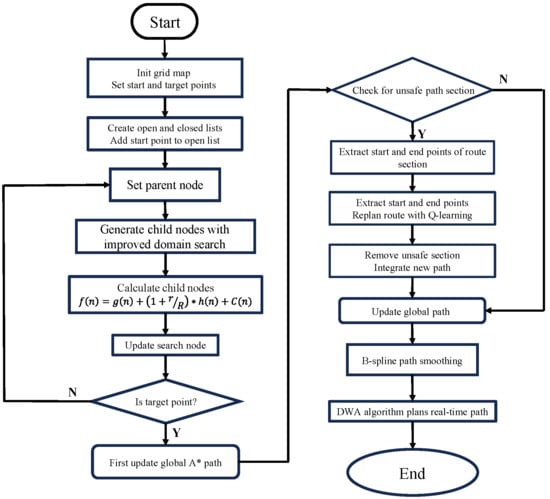
Figure 1.
Optimization algorithm framework.
The procedure begins with the initialization of a grid map and the designation of start and goal points. A global path is then generated using the adaptive A* algorithm. Subsequently, a safety evaluation function is applied to identify any unsafe segments within the initial path. If such segments are detected, they are extracted, and corresponding sub-start and sub-goal points are defined. The Q-learning algorithm is then employed to re-plan these unsafe segments, which are used to replace the original portions of the path.
Finally, the entire path is smoothed using a cubic B-spline curve, and the DWA algorithm is applied for real-time local trajectory planning, ensuring dynamic obstacle avoidance and smooth navigation.
2.1. Optimized A* Algorithm
2.1.1. Traditional A* Algorithm
The A* algorithm is a widely adopted path planning method in robotics, known for its ability to evaluate path costs on grid-based maps. In this representation, black cells denote obstacles, while white cells indicate traversable space. An example of this grid-based environment is shown in Figure 2.
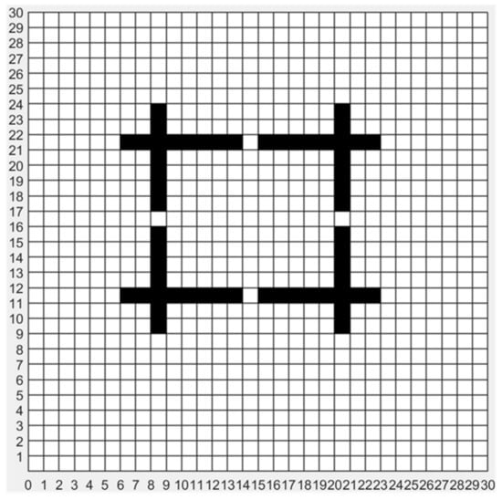
Figure 2.
Grid map environment.
The A* algorithm is widely recognized for its efficiency and effectiveness in robotic path planning. It begins at the initial node, systematically explores neighboring nodes, and employs an evaluation function to select the node with the lowest estimated total cost for expansion. This iterative process continues until the optimal path from the start point to the goal is identified. The evaluation function f(n).used in the A* algorithm is defined in Equation (1):
where g(n) represents the actual cost from the start node to the current node, and h(n) denotes the heuristic estimate of the cost from the current node to the goal.
Commonly used heuristic functions include the Euclidean distance, Manhattan distance, and diagonal distance. In this study, the Euclidean distance is chosen for its higher accuracy and greater likelihood of producing an optimal path. The Euclidean heuristic function is defined in Equation (2):
where (xs, ys) denotes the current node and (xg, yg) denotes the target node.
2.1.2. Adaptive A* Algorithm
To address the limitations of the traditional A* algorithm in path planning—such as poor adaptability to complex and dynamic environments, susceptibility to local optima, and limited safety—this study proposes an enhanced strategy for path optimization. Specifically, to resolve issues including inadequate obstacle clearance, low planning efficiency, insufficient path smoothness, excessive node expansion, and abrupt turning angles, a series of improvements are introduced to the evaluation function, child node selection process, and obstacle avoidance mechanisms:
- (1)
- Optimization of the Evaluation Function
The core of the A* algorithm lies in its evaluation function f(n). The optimization of h(n) is typically the primary focus, as the closer it approximates the true cost-to-go, the more accurate the node selection becomes. However, a more complex heuristic can lead to increased computational overhead due to the expansion of additional nodes, thereby reducing the efficiency of the path planning process. Therefore, selecting an appropriate heuristic function is critical.
By adjusting the relative weighting of g(n) and h(n), the balance between exploration (cost-so-far) and exploitation (cost-to-go) in the A* algorithm can be regulated. If the weight of g(n) is too high, the algorithm may slow down but tend toward the optimal path. Conversely, if the weight of h(n) dominates, the algorithm accelerates but risks losing global optimality. To strike an appropriate balance, the evaluation function is redesigned as follows:
where (1 + r/R) represents the stage-adjusted heuristic weight, R represents the total distance from the starting point to the target point, r represents the distance from the current position to the target point, and C(n) denotes the heading angle function, which is defined to penalize sharp turns.
The term (1 + r/R) theoretically adjusts the heuristic weight based on the search stage:
- When r ≈ R (early stage), (1 + r⁄R) ≈ 2, enhancing the heuristic dominance to accelerate global exploration;
- When r 0 (near goal), (1 + r/R) 1, reducing heuristic impact to prioritize local security.
To reduce the number of turns along the planned path and improve its overall smoothness, a heading angle function C(n) is introduced to evaluate the deviation of a candidate node from the line segment formed by the two preceding nodes. A smaller C(n) value corresponds to a smaller turning angle, thereby contributing to smoother navigation. The value of C(n) is directly related to the turning angle and is normalized to a maximum value of 1. The perpendicular distance function is defined as follows:
where (x1, y1) denotes the previous parent node, (x2, y2) denotes the current parent node, and (x0, y0) denotes the candidate child node.
This design adheres to the principle of heuristic admissibility [16], as the weight assigned to the heuristic component never exceeds the actual cost ratio. As a result, the algorithm maintains optimality while improving overall planning efficiency. Figure 3 illustrates the variation in the weighting factor on a 50 × 50 grid map.
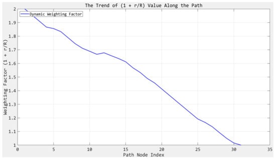
Figure 3.
Curve of the weighting factor (1 + r/R).
- (2)
- Dynamic Connectivity Selection for Child Node Sampling.
In the A* algorithm, the selection of child nodes is based on the evaluation function f(n), while the neighborhood connectivity pattern directly determines the number of redundant nodes generated. Traditional A* algorithms usually adopt fixed 8-connectivity or 16-connectivity methods, as illustrated in Figure 4a,b; however, both fixed patterns have drawbacks: 8-connectivity tends to generate paths with frequent sharp turns and still samples nodes in irrelevant directions, while 16-connectivity, although reducing the number of turns, leads to an exponential expansion of the search space and computational complexity.
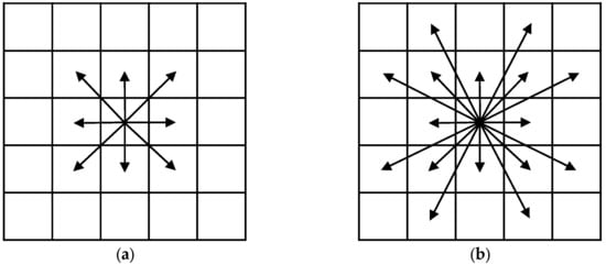
Figure 4.
Connectivity methods: (a) the 8-connectivity method is used for node expansion; (b) the 16-connectivity method is used for node expansion.
To address the limitations of fixed neighborhood sampling in traditional path planning algorithms, this study proposes a dynamic connectivity selection strategy rooted in information entropy theory and motion continuity principles. This strategy adaptively adjusts the neighborhood sampling range (switching among 5-, 8-, 13-, and 16-connectivity) by evaluating environmental uncertainty (including obstacles around the current parent node, robot movement direction, and target direction): in low-entropy scenarios (e.g., no obstacles in the “inner circle”), it adopts 5-connectivity to focus on the primary movement quadrant and avoid redundant sampling; in high-entropy environments (e.g., obstacles in the inner circle), it expands to 16-connectivity to maximize surrounding space information gain. This real-time, locally adaptive mechanism, guided by entropy, theoretically reduces the search space by approximately 30% while maintaining path optimality, with its effectiveness supported by the principle of minimal entropy search [23,24].
In this method, the current parent node is the origin of an X–Y coordinate system divided into four quadrants (Figure 5a): the robot’s movement direction is determined by its relative position to the previous parent node (to confirm the movement quadrant), and the target direction by its relative position to the current parent node. Meanwhile, the eight nodes around the current parent node form an “inner circle,” and the sixteen nodes adjacent to these eight form an “outer circle” (Figure 5b).
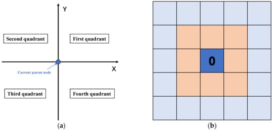
Figure 5.
Schematic diagram: (a) the division of four quadrants, where the center point is the current parent node; (b) the inner ring is highlighted in light brown, and the outer ring is highlighted in light blue. The current parent node is represented by a blue square marked with ‘0’.
During the path planning phase, the algorithm first evaluates whether obstacles exist in the inner circle, and then combines the current movement direction and the target point direction to determine the node search range. As illustrated in Figure 6, the node search ranges under different scenarios are demonstrated and all use one of the cases as a demonstration.
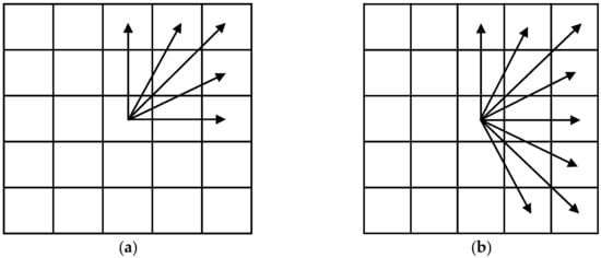
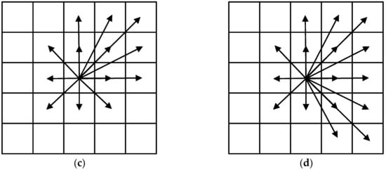
Figure 6.
Schematic diagram of search methods: (a) When there are no obstacles in the inner circle and both the moving direction and the target point direction are in the first quadrant, the 5-connectivity method is employed. (b) When there are no obstacles in the inner circle and the moving direction is in the first quadrant while the target point direction is in the fourth quadrant, the 8-connectivity method is employed. (c) When obstacles exist in the inner circle and both the moving direction and the target point direction are in the first quadrant, the 13-connectivity method is employed. (d) When obstacles are present in the inner circle and the moving direction is in the first quadrant while the target point direction is in the fourth quadrant, the 16-connectivity method is employed.
The algorithm defines environmental uncertainty through “Inner Circle” obstacle detection, locates the primary movement quadrant and target direction, implements adaptive connectivity switching to focus on this primary quadrant (which involves adaptively switching between connectivity patterns based on real-time obstacle data), quantifies the reduction in redundant sampling, and thereby enhances computational efficiency in obstacle-free regions while maintaining safety in complex and cluttered environments. By dynamically limiting the sampling directions to the movement-preferred quadrant—identified from the robot’s heading vector—the algorithm significantly reduces unnecessary node expansion in regions unlikely to contribute to optimal paths.
- (3)
- Obstacle Avoidance Optimization of the A* Algorithm
After generating its child nodes, the A* algorithm evaluates each node using the cost function. If a child node lies within an obstacle, it is excluded from further consideration. Otherwise, the algorithm selects the child node with the lowest evaluation function value to extend the search path. However, the generated paths may fail to maintain a safe distance from obstacles, highlighting the need for improved obstacle avoidance mechanisms, as shown in Figure 7. In the illustrations, the brown triangle represents the robot’s starting position, the green circle marks the target point, and the blue line segments depict the planned trajectory.
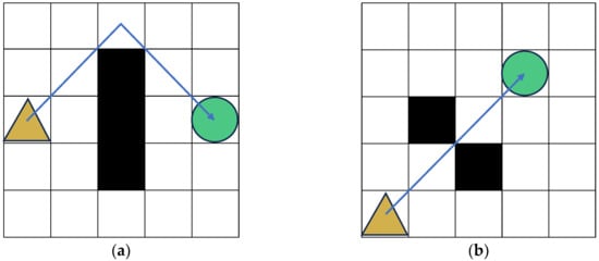
Figure 7.
Risky path diagram: (a) collision with vertices of obstacles during path planning; (b) traversal through adjacent obstacles during path planning.
To enhance the A* algorithm’s path safety, its child node selection is made risk-sensitive, with core optimizations as follows:
When generating child nodes from a parent node, the algorithm first checks if there are obstacles in the 8-neighborhood of the parent node. If obstacles exist, it constructs a line segment L connecting the parent node to each candidate child node. It then calculates the perpendicular distance d between each obstacle in the 8-neighborhood and line segment L. Candidate child nodes where d is smaller than a preset collision safety threshold are discarded.
This modification avoids the robot diagonally crossing obstacle vertices, thereby reducing collision risks and improving navigation safety, as illustrated in Figure 8.
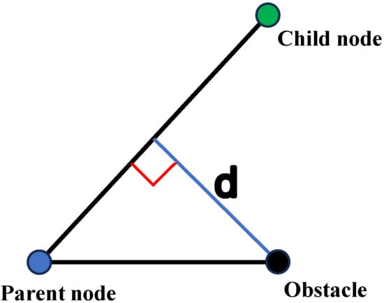
Figure 8.
Distance from line segment L to obstacles.
Equation (7) is the safety distance constraint function (which defines the perpendicular distance from a point to a line); when the distance d from an obstacle to the line segment connecting the parent node and the child node is below the safety threshold, the child node is no longer considered.
where (x1, y1) denotes the current parent node, (x2, y2) denotes the candidate child node, and (x0, y0) denotes the position of the obstacle point.
Through the optimization of child node selection, the adaptive A* algorithm effectively mitigates collision risks and significantly enhances the safety and reliability of robotic path planning, as illustrated in Figure 9.
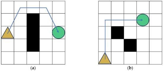
Figure 9.
Optimized path diagram: (a) optimizing the path to safely pass through the vertices of obstacles; (b) optimizing the path to safely navigate through adjacent obstacles.
2.2. Path Smoothing Based on B-Splines
When using a grid map for path planning, the resulting path often contains numerous sharp turns and large steering angles, which are unsuitable for practical engineering applications. B-spline-based path smoothing offers several advantages, including geometric invariance and affine invariance, which help minimize the deviation between the fitted curve and the original discrete path. To address the low safety margin often associated with the classic A* algorithm, the child node selection strategy has also been optimized.
The B-spline curve function is defined as follows:
where Pi represents the coordinates of the control points, Hj,k is the B-spline basis function of degree k, and u is a normalized, non-decreasing knot vector of length n + k + 1. The basis function is a piecewise polynomial of degree k, determined by the knot vector u.
The basis functions are typically computed using the Cox–de Boor recursive formula as follows:
where j denotes the node index, k indicates the order of the basis function, xj denotes the current node, and xj+1 denotes the next node.
Equation (9) defines the zeroth-order basis function, while Equation (10) recursively defines higher-order basis functions from order 1 up to k.
2.3. Path Optimization Using the Q-Learning Algorithm
2.3.1. Introduction to the Q-Learning algorithm
Q-learning, a classical model-free reinforcement learning algorithm, has demonstrated strong performance in robotic path planning and obstacle avoidance tasks. By leveraging simulation platforms such as MATLAB 2024b, Q-learning enables agents to autonomously learn optimal navigation policies through iterative interactions with the environment, without relying on prior environmental knowledge.
This adaptive framework dynamically balances exploration and exploitation, allowing agents to generate collision-free paths in complex and uncertain scenarios. An example of this process is illustrated in Figure 10.
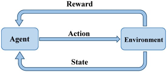
Figure 10.
Schematic diagram of the core logic of the interaction between the agent and the environment.
From a theoretical perspective, Q-learning is an off-policy algorithm within the class of temporal difference (TD) learning methods. It operates under the framework of a Markov Decision Process (MDP)—a mathematical model for sequential decision-making problems, formally defined by the tuple (S, A, P, R) (S: state space, A: action space, P: state transition dynamics, R: reward function) for path planning scenarios.
- (1)
- State Space (S):
The robot’s state st ∈ S at time t is characterized by
where (xt, yt) denotes the robot’s grid coordinates, and Ot ∈ {0, 1} is a binary vector encoding obstacle presence in the 8-neighborhood (0: free, 1: occupied).
- (2)
- Action Space (A):
The robot selects actions at ∈ S from a discrete set of 8 possible movements:
Each action corresponds to a transition to an adjacent grid cell.
- (3)
- State Transition Dynamics (P):
The transition probability P(st+1|st,at) is deterministic in static environments.
where (Δx, Δy) defines the displacement for action at.
- (4)
- Reward Function (R):
The immediate reward rt is designed to balance safety, efficiency, and goal-directed behavior.
where is the Euclidean distance to the goal, and λ = 0.2 weights the distance penalty.
During algorithm execution, the agent records the expected long-term return of each state–action pair by maintaining a Q-value table, which serves as an empirical knowledge base accumulated through environmental interaction. The dynamic update mechanism of the Q-table reflects the core learning logic of the algorithm. When the agent takes an action a in state s, it observes an immediate reward r and transitions to a new state s′. The system then updates the corresponding Q-value based on the temporal difference (TD) error. The Q-value is updated according to the following equation:
where s denotes the current state, a denotes the current action, s’ denotes the next state generated, a′ denotes the next action generated, γ denotes the discount factor that determines the importance of future rewards, r denotes the immediate reward obtained after executing action a′, α represents the learning rate controlling the extent to which new information overrides old estimates, Q(s, a) denotes the Q-value corresponding to taking action a in state s, and maxa ′Q(s′, a′) denotes the maximum estimated Q-value over all possible actions a’ in the next state s′.
Unlike model-based reinforcement learning approaches (e.g., Dyna-Q), the Q-learning implementation adopted in this study is model-free, meaning it learns optimal policies directly through interaction with the environment without requiring a model of environmental dynamics. This design choice aligns with recent advances in uncertainty-aware path planning [18], where model-free policies have demonstrated superior adaptability to sensor noise and dynamic obstacles.
The balance between exploration (achieved via the ε-greedy strategy) and exploitation (through Q-value maximization) in Equation (15) reflects the same trade-off pursued in bio-inspired algorithms [19], but with significantly lower computational complexity, making it well suited for real-time robotic control applications.
2.3.2. Q-Learning Algorithm for Path Optimization of the A* Algorithm
Though the A* algorithm ensures the optimal path length in many cases, its paths may lack sufficient safety margins in complex environments. To solve this, this study uses Q-learning to re-plan unsafe segments of A*-generated paths for better overall safety.
First, the A*-generated path is evaluated to check each node’s distance to the nearest obstacle; consecutive nodes within a predefined safety threshold (e.g., ≤2 grid units) mark the segment as unsafe. The last safe node before this segment is set as the sub-start point, and the first safe node after it as the sub-goal point. Then, Q-learning re-plans the path between the sub-start and sub-goal points (treating the unsafe segment as a local re-planning task), and the new segment replaces the original unsafe one—resulting in a trajectory that retains global optimality while improving local safety.
2.4. DWA Algorithm
The DWA algorithm dynamically determines a robot’s linear velocity and steering angle based on its current motion state and surrounding environment. At each time step, it calculates potential trajectories under different velocity and direction combinations, evaluates them via a cost function, and selects the lowest-cost one as the next action plan [25]. It is highly effective for dynamic and unknown static obstacles, enabling real-time trajectory adjustment to ensure smooth obstacle avoidance while moving efficiently toward the target. This paper uses a differential drive model (robot moves forward with linear velocity v along the x-axis and rotates with angular velocity ω about the z-axis), and approximates the trajectory between adjacent points as a straight line in short (millisecond-scale) time intervals.
The actual distance Δs traveled by the robot over a time interval Δs is given by Δs = v × Δt.
Converting this into Cartesian coordinates yields the following:
Accordingly, the robot’s state at the next time step is computed as follows:
where θt denotes the heading angle at time t.
3. Experiments
3.1. Experimental Environment
To validate the proposed algorithm’s improvements, a dual-group experiment with controlled environments was conducted:
- Group 1 used four map sizes (30 × 30 to 200 × 200) with 10% obstacle density (fixed MATLAB random seeds rng (1)–rng (10) for consistent setups across 10 trials per map);
- Group 2 used a fixed 50 × 50 map with obstacle densities varying 0–20% (seed-controlled distributions).
Both algorithms ran 10 independent times per configuration to compare search time, path length, node efficiency, and safety metrics (e.g., number of unsafe nodes). Performance trade-offs were measured via path length ratios (improved vs. traditional) and node reduction rates. This design isolated scalability (Group 1) and obstacle resilience (Group 2) under repeatable conditions, ensuring statistical rigor (mean ± standard deviation) and real-world simulation accuracy.
The experimental setup used MATLAB 2024b on a computer equipped with an Intel Core i5-8300H CPU (manufactured by Intel Corporation, Santa Clara, CA, USA) and Kingston 16 GB of RAM (Fountain Valley, CA, USA), and Micron (Boise, ID, USA), ensuring compliance with standard simulation protocols. The learning rate α = 0.1 was chosen to balance learning stability and convergence efficiency, preventing policy oscillations caused by excessive parameter values, while the discount factor γ = 0.9 was adopted to enhance the preference for long-term safe paths, and the exploration rate ε = 0.2 balances the exploration–exploitation trade-off, enabling the algorithm to prioritize globally optimal trajectories that bypass obstacles [16]. The DWA algorithm operated with a linear velocity v ∈ [0, 1.5] m/s, angular velocity ω ∈ [−1.5, 1.5] rad/s, and a prediction time window Δt = 0.5 [12].
3.2. Simulation Experiments of the Adaptive A* Algorithm
3.2.1. Simulation Experiments with Different Map Sizes
This simulation experiment used four grid maps of different sizes, all with a fixed 10% obstacle density (chosen for balanced complexity—more challenging than 5% but more manageable than 15%/20%, enabling timely path planning and serving as a good evaluation benchmark). For each map size, both the traditional A* and adaptive A* algorithms underwent 10 independent tests under identical environments and initial conditions (to eliminate randomness and boost result robustness). During testing, scenarios of obstacle-blocked paths requiring dynamic re-planning were observed, and key indicators (search time, path length, number of path nodes, and number of unsafe nodes—proportion of nodes within ≤1 grid unit of the nearest obstacle) were recorded for each algorithm.
The start and goal coordinates were defined separately for each map size as follows:
- 30 × 30 map: start point = (3, 3); goal point = (28, 28).
- 50 × 50 map: start point = (3, 3); goal point = (48, 45).
- 100 × 100 map: start point = (3, 3); goal point = (95, 95).
- 200 × 200 map: start point = (3, 3); goal point = (195, 195).
The simulation results are shown in Table 4.

Table 4.
Experimental data of traditional and adaptive A* algorithm.
3.2.2. Simulation Experiments with Different Obstacle Rates
The previous experimental analysis demonstrated that, on maps with a 10% obstacle density, the adaptive A* algorithm produces paths that are approximately 10% longer than those generated by the traditional A* algorithm, while reducing the number of expanded nodes by roughly 30%. These observations are largely attributed to the improved node selection and obstacle avoidance mechanisms. It is reasonable to hypothesize that variations in obstacle density may influence these two performance factors.
To validate this hypothesis, a series of experiments was conducted on a 50 × 50 grid map with varying obstacle densities. For each configuration, the path length and number of search nodes were recorded for both algorithms. The mean values of these metrics were then computed across 10 independent runs. To enable a comparative analysis, the ratios of path lengths and node quantities between the improved and traditional algorithms were calculated. The start and goal point coordinates were set to (3, 3) and (48, 45), respectively. A summary of the experimental data is provided in Table 5.

Table 5.
Comparison of result parameters at different obstacle rates.
The 50 × 50 map size was selected because it reflects the complexity commonly encountered in practical robotic navigation tasks. Therefore, the results of this experiment provide valuable insights into the algorithm’s performance and applicability in real-world environments.
4. Results Analysis and Discussion
4.1. Simulation Data Analysis
4.1.1. Performance of the Adaptive A* Algorithm Under Varied Map Sizes
Table 4 presents the results of the first group of simulation experiments on grid maps of different sizes. Compared with the traditional A* algorithm, the adaptive A* algorithm generates paths approximately 10% longer but reduces the number of expanded nodes by about 30%. In terms of search time, the two algorithms perform similarly only on the smallest map (30 × 30); for larger maps (50 × 50 to 200 × 200), the adaptive A* algorithm shortens the search time by 10–20%. In terms of safety, the proportion of unsafe nodes (defined as nodes with a distance of ≤1 grid unit from the nearest obstacle) of the adaptive A* algorithm is reduced by 35–50%, and the path safety improvement is particularly significant in larger and more complex environments.
4.1.2. Performance of the Adaptive A* Algorithm Under Varied Obstacle Densities
Table 5 shows the results of the second group of experiments focusing on algorithm performance under different obstacle densities. When the obstacle density is 0% or 5%, the path lengths generated by the two algorithms are nearly the same; when the density reaches 10% or higher, the adaptive A* algorithm produces noticeably longer paths. This is due to its optimized node selection and obstacle avoidance mechanisms, which adopt more conservative detour strategies to ensure path safety in complex environments. Even in environments with a high obstacle density, the adaptive A* algorithm still uses fewer nodes than the traditional A* algorithm and reduces node expansion during the search process, thereby improving overall search efficiency.
4.1.3. Optimization Mechanism and Safety Improvement of the Adaptive A* Algorithm
The adaptive A* algorithm achieves a reduced runtime and fewer nodes by integrating dynamic heuristic weighting and entropy-driven switching among 5-neighborhood, 8-neighborhood, 13-neighborhood, and 16-neighborhood sampling, though its performance varies with the map environment. For example, when the obstacle density is 5%, the traditional A* algorithm expands 45 nodes through fixed eight-neighborhood sampling, while the adaptive algorithm reduces the number of nodes to 23 (Table 5) via entropy-based five-neighborhood focusing, minimizing 70% of invalid searches. When the obstacle density is ≥5%, the algorithm enforces detours through Equation (7): for instance, in a 50 × 50 map with 20% obstacle density, the path length increases from 63.54 to 75.46; in 30 × 30 to 200 × 200 maps with 10% obstacle density, the path length growth remains stable at 10% ± 1, indicating that path elongation is only affected by obstacle density. Meanwhile, the adaptive A* algorithm achieves significant safety improvements: in a 50 × 50 map with 20% obstacle density, the number of unsafe nodes decreases by 40% ± 5; in a 200 × 200 map with 10% obstacle density, the number of unsafe nodes reduces by 50% ± 5.
In larger maps ranging from 50 × 50 to 200 × 200, the adaptive A* consistently maintained safety by reducing unsafe nodes by up to 52%, while optimizing search time and minimizing redundant node expansion.
4.2. Performance Comparison of the Adaptive A* Algorithm
Taking a 30 × 30 grid map as an example—where each cell is a square with a side length of 1 unit—the experimental results of path planning using both the traditional and adaptive A* algorithms are presented in Figure 11, with the blue lines representing the planned paths.
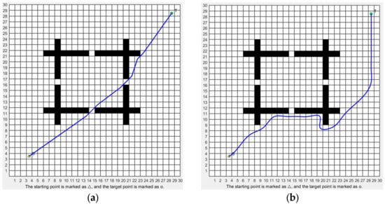
Figure 11.
Experimental comparison between the traditional A* algorithm and the adaptive A* algorithm on a 30 × 30 grid map: (a) path generated by the traditional A* algorithm; (b) path generated by the adaptive A* algorithm.
A direct comparison under identical environmental conditions reveals that the path generated by the adaptive A* algorithm exhibits smaller turning angles and maintains a greater distance from obstacles, resulting in improved safety. In particular, the improved algorithm provides a wider buffer zone around the robot’s trajectory, reducing the likelihood of collisions during navigation.
This enhanced safety performance comes at the cost of a moderate increase in path length. Since the adaptive A* algorithm explicitly prioritizes path smoothness and obstacle clearance, it naturally sacrifices some path optimality in terms of distance. Nevertheless, the trade-off is justified by the significant improvements in navigation safety and overall path quality.
4.3. Q-Learning Algorithm Path Optimization Simulation Experiment
Due to the nature of the adaptive A* algorithm itself, in path planning, there will be trajectories that are close to the obstacle boundaries, and there are potential safety risks during the execution process. To address this issue, the Q-learning algorithm is applied to locally optimize the path, as illustrated in Figure 12, with the blue lines representing the planned paths This local re-planning process allows the agent to generate an alternative path that increases obstacle clearance while maintaining overall trajectory continuity and goal orientation.
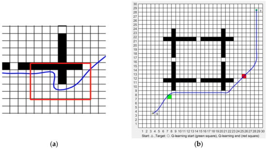
Figure 12.
Local path optimization using the Q-learning algorithm: (a) local view of the path generated by the adaptive A* algorithm (from Figure 11b), including the unsafe segments.; (b) re-planned segment using Q-learning, improving safety by increasing clearance from nearby obstacles.
4.4. Simulation Experiments with the Integration of the DWA Algorithm
The DWA is a highly responsive and adaptable local path planning algorithm capable of adjusting a robot’s motion trajectory in real time. When the robot encounters dynamically changing environments, the DWA algorithm can promptly modify the robot’s linear and angular velocities to effectively navigate around moving obstacles and adapt to environmental changes.
To enhance overall path safety and adaptability, the adaptive A* algorithm, Q-learning algorithm, and DWA algorithm are integrated to address the challenges of mobile obstacle avoidance and unknown static obstacle detection for spraying robots. The real-time obstacle avoidance capability of the integrated system is evaluated by adding one moving obstacle and one unknown static obstacle to the original path.
Since DWA operates as a local planner, capable of dynamically re-planning paths upon encountering unsafe segments, a comparative simulation was conducted, as illustrated in Figure 13, with the blue lines representing the planned paths.
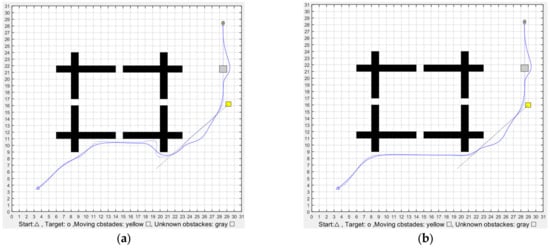
Figure 13.
Optimization of the DWA algorithm: (a) integration of the adaptive A* algorithm and the DWA algorithm; (b) integration of the adaptive A* algorithm, Q-learning algorithm, and DWA algorithm.
The results demonstrate that the robot can effectively avoid both moving and previously unknown static obstacles, achieving autonomous navigation in real-time conditions. Compared with the original planned path, the actual path is smoother and exhibits better adaptability to environmental changes. It is noteworthy that the fusion algorithm integrated with the Q-learning algorithm yields a longer path featuring fewer sharp turns, emphasizing greater obstacle clearance and safety. This suggests that integrating Q-learning with the adaptive A* and DWA algorithms enhances the system’s ability to generate smoother, safer paths under complex, dynamic conditions.
4.5. Experimental Results Analysis
Based on the results of extensive simulation experiments, five key factors contributing to path optimization have been identified:
- (1)
- Evaluation Function Enhancement:
By dynamically adjusting the weight of the heuristic component, the number of expanded nodes during the planning process can be significantly reduced. As the robot approaches the target, the algorithm continuously optimizes the path to improve both smoothness and safety, thereby reducing computational load and enhancing planning efficiency.
- (2)
- Optimized Child Node Selection:
The algorithm evaluates three conditions—the presence of obstacles in the inner circle, the direction of movement, and the direction of the search—to adaptively choose the most appropriate connectivity pattern among four options. Combined with an obstacle avoidance mechanism, this approach allows dynamic strategy switching based on the local environment, enhancing both path safety and search efficiency.
- (3)
- Unsafe Path Re-planning:
Sections of the initial path generated by the adaptive A* algorithm that are deemed unsafe in complex environments are re-planned using the Q-learning algorithm. This re-planning process significantly improves the safety of the final trajectory.
- (4)
- Path Smoothing:
The use of cubic uniform B-spline curves for post processing reduces sharp turning angles along the path, improving the smoothness and stability of the robot’s motion.
- (5)
- Handling of Unknown Obstacles:
The DWA algorithm is incorporated to handle both moving and previously unknown static obstacles in real time, ensuring adaptive navigation and enhancing the robot’s operational safety.
Through the integration of the adaptive A* algorithm, Q-learning, and DWA, the proposed framework achieves a balanced solution that ensures safe path planning for spraying robots while also improving operational efficiency and motion stability.
4.6. Uncertainty Analysis and Coping Strategies
Although the algorithm has demonstrated strong performance in simulations, real-world applications are subject to internal and external uncertainties that may compromise path safety and execution accuracy.
4.6.1. Internal Uncertainties
- (1)
- Sensor Noise:
LiDAR ranging errors (±2 cm) can lead to inaccurate obstacle modeling, potentially violating safety distance constraints. For example, a 10 cm gap may be misclassified as 15 cm, resulting in unsafe path segments [1,2].
- (2)
- Motion Model Errors:
The differential drive system of the robot may introduce turning radius deviations (average 3–5 cm), causing discrepancies between the planned and actual paths.
- (3)
- Mitigation Strategy:
The Uncertainty-Aware Safe Trajectory Planner (UA-MPC-CBF) models these noise and motion uncertainties using a probabilistic boundary framework [26]. Even under complex internal disturbances, this method achieves 99.9% feasibility for safe path planning, thereby significantly improving robustness.
To further mitigate internal uncertainties during navigation, especially under sensor noise or partial observability, we propose three optimization strategies:
- The EKF (Extended Kalman Filter) fusion of LiDAR and monocular vision, which reduces the ranging error to ±0.8 cm and increases the safety threshold when the obstacle confidence is low;
- The correction of turning costs using the dynamic error coefficient β based on historical motion data (expressed as C’(n) = β × C(n));
- The reduction in the heuristic weight when the sensor confidence is low (decreasing 1 + r/R from 2 to 1.2).
4.6.2. External Uncertainties
- (1)
- Randomness of Dynamic Obstacles:
Pedestrians exhibit random speed (0.5–1.5 m/s) and direction changes. These violate the constant velocity assumption in DWA’s velocity obstacle model, leading to local oscillations in approximately 20% of observed cases.
- (2)
- Inaccurate Environmental Modeling:
In unstructured environments such as farmland, small obstacles (<10 cm) are often undetectable in grid-based maps, leading to navigation failures in around 15% of cases where paths intersect with unmodeled terrain features.
- (3)
- Mitigation Strategies:
Robust Reinforcement Learning (RRL) [18]: By incorporating disturbance-resilient reward functions (e.g., penalizing abrupt speed fluctuations), RRL can reduce path oscillations by up to 80%.
5. Conclusions
Compared with the traditional A* algorithm and existing hybrid approaches [12,13,14,16,17], the proposed adaptive A*–Q-Learning–DWA hybrid algorithm for spraying robots offers key advantages. Traditional A* relies on fixed heuristic functions and static neighborhood exploration (e.g., fixed 8- or 16-connectivity), causing redundant node expansion and poor dynamic adaptability; the proposed algorithm addresses this via dynamic heuristic weighting (adjusted by distance to the target) and adaptive connectivity switching (5-, 8-, 13-, or 16-connectivity based on environment), reducing redundancy, boosting computational efficiency, and preserving global optimality. Existing hybrid methods like DP-A* [16] and GAA-DFQ [17] depend on predefined environmental models, limiting unknown scenario adaptability, while the proposed algorithm uses Q-learning for real-time unsafe segment re-planning without a priori knowledge. Methods integrating only local planners (e.g., DWA [22]) lack global foresight and fall into local minima in cluttered environments, but the proposed fusion of adaptive A* (global planning), Q-learning (local re-planning), and DWA (real-time obstacle avoidance) mitigates such issues and enhances obstacle negotiation.
The algorithm also has practical limitations. Stricter safety criteria (e.g., obstacle clearance) lead to longer paths, potentially lowering efficiency for time-sensitive tasks. In high-obstacle-density environments, dynamic heuristic adjustment and adaptive exploration increase computational complexity, threatening real-time performance. Real-world deployment is further challenged by internal uncertainties (sensor inaccuracies, actuator delays) and external uncertainties (random dynamic obstacle movements, inaccurate environmental modeling). Future work will integrate probabilistic methods, robust reinforcement learning, and enhanced real-time perception to improve robustness and expand the applicability to real-world spraying robot path planning in underground coal mines.
Author Contributions
Conceptualization, C.S. and L.Z.; methodology, C.S. and L.Z.; software, L.Z.; validation, L.Z. and D.X.; formal analysis, C.S.; resources, C.S.; data curation, L.Z.; writing—original draft preparation, L.Z.; writing—review and editing, L.Z. and D.X.; visualization, D.X.; supervision, C.S.; project administration, C.S.; funding acquisition, C.S. All authors have read and agreed to the published version of the manuscript.
Funding
This work was supported by the National Natural Science Foundation of China (Grant No. 52374156).
Data Availability Statement
The datasets utilized and/or analyzed during the current study are available from the corresponding author on reasonable request.
Conflicts of Interest
The authors declare no conflicts of interest.
References
- Li, C.; Zhang, X. Operation technology of unmanned mining robot for coal mine based on intelligent control technology. In Proceedings of the 2023 International Conference on Computer Simulation and Modeling, Information Security (CSMIS), Buenos Aires, Argentina, 15–17 November 2023; IEEE: Piscataway, NJ, USA, 2024; pp. 86–91. [Google Scholar]
- Liu, Z. Navigation system of coal mine rescue robot based on virtual reality technology. In Proceedings of the 2022 World Automation Congress (WAC), San Antonio, TX, USA, 11–15 October 2022; IEEE: Piscataway, NJ, USA, 2022; pp. 379–383. [Google Scholar]
- Zhang, H.; Xie, X.; Wei, M.; Wang, X.; Song, D.; Luo, J. An improved goal-bias RRT algorithm for unmanned aerial vehicle path planning. In Proceedings of the 2024 IEEE International Conference on Mechatronics and Automation (ICMA), Tianjin, China, 4–7 August 2024; IEEE: Piscataway, NJ, USA, 19 August, 2024; pp. 1360–1365. [Google Scholar]
- Fu, S. Robot Path Planning Optimization Based on RRT and APF Fusion Algorithm. In Proceedings of the 2024 8th International Conference on Robotics and Automation Sciences (ICRAS), Tokyo, Japan, 21–23 June 2024; IEEE: Piscataway, NJ, USA, 2024; pp. 32–36. [Google Scholar]
- Zhu, W.; Qiu, G. Path Planning of Intelligent Mobile Robots with an Improved RRT Algorithm. Appl. Sci. 2025, 15, 3370. [Google Scholar] [CrossRef]
- Wu, D.; Li, Y. Mobile Robot Path Planning Based on Improved Smooth A* Algorithm and Optimized Dynamic Window Approach. In Proceedings of the 2024 2nd International Conference on Signal Processing and Intelligent Computing (SPIC), Guangzhou, China, 20–22 September 2024; IEEE: Piscataway, NJ, USA, 2024; pp. 345–348. [Google Scholar]
- Meng, F.; Sun, X.; Zhu, J.; Mei, B.; Zheng, P. Research on Ship Path Planning Based on Bidirectional A*-APF Algorithm. In Proceedings of the 2024 4th International Conference on Consumer Electronics and Computer Engineering (ICCECE), Guangzhou, China, 12–14 January 2024; 2024; pp. 460–466. [Google Scholar]
- Fu, B.; Chen, L.; Zhou, Y.; Zheng, D.; Wei, Z.; Dai, J.; Pan, H. An improved A* algorithm for the industrial robot path planning with high success rate and short length. Robot. Auton. Syst. 2018, 106, 26–37. [Google Scholar] [CrossRef]
- Lv, Y.; Wang, J.; Yang, H.; Zhang, X. Dynamic Guidance Point Obstacle Avoidance Planning Method and Optimization Based on DWA. In Proceedings of the 2024 International Conference on Cyber-Physical Social Intelligence (ICCSI), Doha, Qatar, 8–12 November 2024; IEEE: Piscataway, NJ, USA, 2024; pp. 1–6. [Google Scholar]
- Nie, W.; Fu, H.; Ma, S.; Deng, Y.; Yang, J. An Improved FFPF-APF Path Planning. In Proceedings of the 4th 2024 International Conference on Autonomous Unmanned Systems (4th ICAUS 2024): Volume II, Shenyang, China, 19–21 September 2024; Springer Nature: Berlin/Heidelberg, Germany, 2025; Volume 1375, pp. 156–170. [Google Scholar]
- Zhang, H.M.; Li, M.L.; Yang, L. Safe path planning of mobile robot based on improved A* algorithm in complex terrains. Algorithms 2018, 11, 44. [Google Scholar] [CrossRef]
- Zhang, J.; Ling, H.; Tang, Z.; Song, W.; Lu, A. Path planning of USV in confined waters based on improved A∗ and DWA fusion algorithm. Ocean. Eng. 2025, 322, 120475. [Google Scholar] [CrossRef]
- Fu, X.; Huang, Z.; Zhang, G.; Wang, W.; Wang, J. Research on path planning of mobile robots based on improved A* algorithm. PeerJ Comput. Sci. 2025, 11, e2691. [Google Scholar] [CrossRef] [PubMed]
- Jing, M.; Wang, H. Robot path planning by integrating improved A* algorithm and DWA algorithm. J. Phys. Conf. Ser. 2023, 492, 012017. [Google Scholar]
- Huang, X.; Li, G. An improved Q-learning algorithm for path planning. In Proceedings of the 2023 IEEE International Conference on Sensors, Electronics and Computer Engineering (ICSECE), Jinzhou, China, 18–20 August 2023; IEEE: Piscataway, NJ, USA, 2023; pp. 277–281. [Google Scholar]
- Gan, X.; Huo, Z.; Li, W. Dp-a*: For path planing of ugv and contactless delivery. IEEE Trans. Intell. Transp. Syst. 2023, 25, 907–919. [Google Scholar] [CrossRef]
- Liao, C.; Wang, S.; Wang, Z.; Zhai, Y. GAA-DFQ: A dual-layer learning model for robot path planning in dynamic environments integrating genetic algorithms, DWA, fuzzy control and Q-learning. In Proceedings of the 2025 8th International Conference on Advanced Algorithms and Control Engineering (ICAACE), Shanghai, China, 21–23 March 2025; IEEE: Piscataway, NJ, USA, 2025; pp. 339–343. [Google Scholar]
- Hwang, U.; Hong, S. On Practical Robust Reinforcement Learning: Adjacent Uncertainty Set and Double-Agent Algorithm. IEEE Trans. Neural Netw. Learn. Syst. 2024, 36, 7696–7710. [Google Scholar] [CrossRef] [PubMed]
- De Carvalho, K.B.; de OBBatista, H.; Fagundes-Junior, L.A.; de Oliveira, I.R.L.; Brandão, A.S. Q-learning global path planning for UAV navigation with pondered priorities. Intell. Syst. Appl. 2025, 25, 200485. [Google Scholar] [CrossRef]
- Lu, Y.; Da, C. Global and local path planning of robots combining ACO and dynamic window algorithm. Sci. Rep. 2025, 15, 9452. [Google Scholar] [CrossRef] [PubMed]
- Du, X.; Luo, P.; Lv, X. Path Planning Algorithm Based on Improved RRT and Artificial Potential Field. In Proceedings of the 2024 8th International Conference on Electrical, Mechanical and Computer Engineering (ICEMCE), Xi’an, China, 25–27 October 2024; pp. 1767–1774. [Google Scholar]
- Liu, Y.T.; Guo, S.J.; Tang, S.F.; Zhang, X.W.; Li, T.T. Path planning based on fusion of improved A* and ROA-DWA for robot. Zhejiang Daxue Xuebao (Gongxue Ban)/J. Zhejiang Univ. (Eng. Sci.) 2024, 58, 360–369. [Google Scholar]
- Wang, P.; Gupta, K. View planning via maximal c-space entropy reduction. In Algorithmic Foundations of Robotics V; Springer: Berlin/Heidelberg, Germany, 2004; pp. 149–165. [Google Scholar]
- Lanillos, P.; Besada-Portas, E.; Pajares, G.; Ruz, J.J. Minimum time search for lost targets using cross entropy optimization. In Proceedings of the 2012 IEEE/RSJ International Conference on Intelligent Robots and Systems, Vilamoura, Algarve, Portugal, 7–12 October 2012; IEEE: Piscataway, NJ, USA, 2012; pp. 602–609. [Google Scholar]
- Gong, X.; Gao, Y.; Wang, F.; Zhu, D.; Zhao, W.; Wang, F.; Liu, Y. A local path planning algorithm for robots based on improved DWA. Electronics 2024, 13, 2965. [Google Scholar] [CrossRef]
- Guo, Z.; Chen, H.; Xu, F.; Hu, Y.; Lin, J.; Guo, L. Uncertainty-Aware Safe Trajectory Planner Based on Model Predictive Control for Autonomous Driving. IEEE Trans. Intell. Transp. Syst. 2025, 26, 12068–12079. [Google Scholar] [CrossRef]
Disclaimer/Publisher’s Note: The statements, opinions and data contained in all publications are solely those of the individual author(s) and contributor(s) and not of MDPI and/or the editor(s). MDPI and/or the editor(s) disclaim responsibility for any injury to people or property resulting from any ideas, methods, instructions or products referred to in the content. |
© 2025 by the authors. Licensee MDPI, Basel, Switzerland. This article is an open access article distributed under the terms and conditions of the Creative Commons Attribution (CC BY) license (https://creativecommons.org/licenses/by/4.0/).