Multilingual Mobility: Audio-Based Language ID for Automotive Systems

Abstract

With the growing demand for natural and intelligent human–machine interaction in multilingual environments, automatic language identification (LID) has emerged as a crucial component in voice-enabled systems, particularly in the automotive domain. This study proposes an audio-based LID model that identifies the spoken language directly from voice input without requiring manual language selection. The model architecture leverages two types of feature extraction pipelines: a Variational Autoencoder (VAE) and a pre-trained Wav2Vec model, both used to obtain latent speech representations. These embeddings are then fed into a multi-layer perceptron (MLP)-based classifier to determine the speaker’s language among five target languages: Korean, Japanese, Chinese, Spanish, and French. The model is trained and evaluated using a dataset preprocessed into Mel-Frequency Cepstral Coefficients (MFCCs) and raw waveform inputs. Experimental results demonstrate the effectiveness of the proposed approach in achieving accurate and real-time language detection, with potential applications in in-vehicle systems, speech translation platforms, and multilingual voice assistants. By eliminating the need for predefined language settings, this work contributes to more seamless and user-friendly multilingual voice interaction systems.

1. Introduction

With the increasing adoption of voice-enabled technologies in modern vehicles, natural and seamless interaction between drivers and in-car systems has become essential. However, current systems often rely on a fixed default language, which poses usability challenges for multilingual users. As global mobility expands, there is a growing demand for intelligent in-vehicle systems capable of automatically identifying the speaker’s language and adapting accordingly.

Operating in automotive environments, however, introduces unique acoustic challenges. Factors such as cabin reverberation, engine and road noise, and overlapping speech from multiple occupants significantly degrade the performance of conventional Language Identification (LID) models, which are typically trained on clean, studio-quality speech corpora. Additionally, automotive systems demand real-time, low-latency inference on embedded hardware with limited computational resources—posing further constraints on model design.

In shared vehicle environments, users are often confronted with a default system language that is unfamiliar and difficult to change. Accessing the language settings is typically buried within complex menus, and attempting to modify them while driving can be unsafe and distracting. This challenge is further amplified for users whose native language differs from the default setting. To overcome these limitations, automatic LID systems are essential. However, the in-vehicle environment introduces significant acoustic challenges due to engine noise, road noise, and other external disturbances, which can severely degrade the performance of audio-based LID models.

To address these challenges, we present a noise-robust and computationally efficient audio-based LID model specifically tailored for in-vehicle integration. Our architecture extracts language-relevant embeddings using both a Variational Autoencoder (VAE) and a pre-trained Wav2Vec model, which are then classified by a lightweight multi-layer perceptron. In contrast to previous approaches that rely solely on a single representation, our method fuses self-supervised contextual embeddings with generative latent features to capture both high-level semantic information and fine-grained phonetic structure. This dual-representation strategy enhances the model’s ability to differentiate acoustically overlapping languages under noisy conditions, which is a common limitation in existing LID systems. The system is designed for real-time operation and supports dynamic language switching for functions such as navigation, media playback, and hands-free control. Evaluation is conducted on a multilingual speech dataset under both clean and noisy conditions that simulate real driving environments.

While this work is primarily focused on automotive applications, the proposed approach is also applicable to other domains requiring spontaneous, multilingual interaction. For example, speech-to-speech translation platforms such as Naver’s Papago [1] and Google Translate [2] have gained widespread popularity for enabling real-time language translation in travel and cross-cultural communication. Unlike conventional systems that require manual specification of the source language, our method automatically detects the spoken language directly from the audio signal. This facilitates more intuitive and efficient user experiences by removing the need for explicit language selection.

2. Related Works

Early studies in language identification primarily focused on modeling acoustic and phonotactic characteristics of speech. These approaches were particularly effective in controlled environments such as telephone conversations, where utterance length and signal channel variability significantly impacted performance. Over time, the field has evolved from traditional probabilistic models to more data-driven methods, including deep neural networks and representation learning. This progression reflects a broader trend in speech processing, where handcrafted features have increasingly been complemented or replaced by learned embeddings optimized for specific tasks.

Underlying these advancements is the continuous reliance on meaningful audio representations. Speech features such as Cepstral Coefficients (MFCCs), Perceptual Linear Prediction (PLP) coefficients, and Linear Prediction Cepstral Coefficients (LPCCs) have long served as the foundation for both classical and modern LID systems, capturing the essential spectral and perceptual cues of spoken language. Despite the emergence of end-to-end learning, these features remain relevant, especially in scenarios where data are limited, computation is constrained, or interpretability is required.

2.1. Language Identification Models

Automatic LID technology has been actively studied and applied in telephone speech scenarios, where signal conditions and channel variability pose additional challenges. One of the seminal works in this area, Zissman (1996) [3], compared four approaches to LID on telephone speech data: (1) GMM-based acoustic classification [4], (2) single-language phone recognition followed by interpolated n-gram modeling (PRLM) [5], (3) parallel PRLM using multiple phone recognizers [6], and (4) language-dependent parallel phone recognition (PPR) [7]. These methods combine acoustic and phonotactic modeling, with phonotactic approaches generally outperforming purely acoustic methods. In particular, parallel PRLM achieved the lowest error rates—2% for 45 s and 5% for 10 s utterances in two-language classification, and 11% and 21%, respectively, in 11-language classification tasks. These results underscore the importance of phonotactic information for LID in challenging environments, laying the foundation for many subsequent real-world systems.

More recently, deep neural networks (DNNs) have shown remarkable success in acoustic modeling tasks [8] and have been investigated for language identification. Unlike shallow architectures or convolutional neural networks applied in earlier works, fully connected deep architectures trained on frame-level acoustic features have demonstrated superior discriminative capability, especially when large-scale annotated datasets are available [9]. Experimental comparisons on large corpora, such as the Google 5M LID dataset [10] and NIST LRE 2009 benchmark [11], reveal that DNN-based LID systems can significantly outperform i-vector baselines in both accuracy and calibration metrics. These advances motivate the integration of deep learning approaches for more robust and scalable language identification systems.

2.2. Speech Audio Features

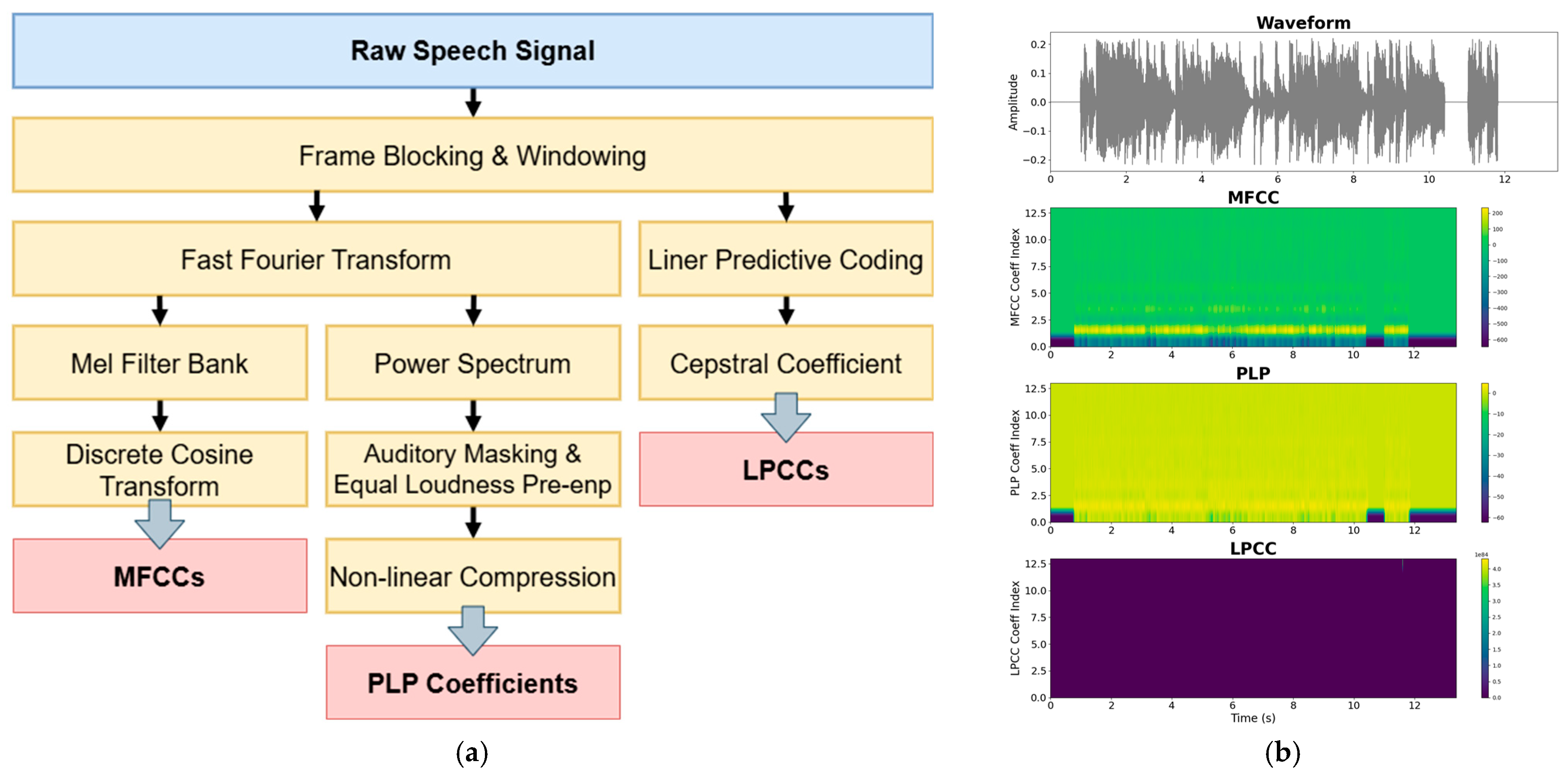
Speech audio features play a crucial role in various speech processing tasks, including speech recognition, speaker identification, and language identification. These features are designed to capture relevant characteristics of the speech signal that reflect its phonetic, acoustic, and perceptual properties. By extracting informative representations from raw audio, speech features enable machine learning models to effectively analyze and interpret spoken language. Commonly used speech audio features include MFCCs, PLP coefficients, and LPCCs, all of which model the speech spectrum in a manner that closely aligns with human auditory perception [12]. Figure 1 illustrates the extraction processes of the three speech audio features, while

Table 1. Audio feature comparison: MFCC, LPCC, and PLP.

Speech Audio Feature
	MFCCS	LPCCs	PLP
Spectral Analysis	FFT + Mel filter bank	FFT + Mel filter bank + LPC	LPC only
Noise Robustness	Moderate	High	Low
Computational Complexity	Moderate	Relatively high	Low
Strength	Widely used	Incorporates human hearing characteristics	Simple, good for modeling vocal tract resonances
Weakness	Sensitive to noise and channel variations	More computationally expensive	Poor performance in noisy environments

provides a comparative analysis of their characteristics.

MFCCs [13] are among the most widely used speech features, designed to model the human auditory system’s nonlinear frequency response. The extraction process begins by dividing the speech signal into short frames, typically 20 to 40 ms in length. Each frame undergoes a Fourier transform to obtain its frequency spectrum, which is then passed through a bank of filters spaced according to the Mel-scale to mimic the critical bands of human hearing. The logarithm of the filter bank energies is computed, followed by a discrete cosine transform (DCT) to decorrelate the features and reduce dimensionality. The resulting coefficients succinctly represent the spectral envelope of the speech and are highly effective in automatic speech recognition tasks.

PLP [14] improves upon MFCC by incorporating additional psychoacoustic models to better simulate human auditory perception. After computing the power spectrum of each speech frame, the signal is filtered using Mel-scaled critical bands, and auditory masking effects are applied to account for the influence of nearby frequencies. Subsequently, the spectrum undergoes equal loudness pre-emphasis and compression. Linear predictive coding (LPC) analysis is then performed to model the spectral envelope, and the LPC coefficients are converted into cepstral coefficients. PLP features have been shown to be more robust to noise and variations in the speech signal compared to MFCC, making them advantageous in challenging acoustic environments.

LPCCs [15] are derived from linear predictive coding of the speech signal without explicitly modeling human auditory perception. The speech signal is segmented into frames, and LPC analysis estimates the vocal tract filter coefficients by minimizing the prediction error. These LPC coefficients are subsequently transformed into cepstral coefficients, which compactly characterize the spectral envelope of speech. While LPCCs effectively capture resonant properties of the vocal tract and are used in speech synthesis and recognition, they lack the perceptual weighting present in MFCC and PLP, which can limit their performance in noisy or real-world conditions.

3. Language Identification Model

To classify languages from speech audio, it is essential to extract salient audio features and represent them as numerical vectors. In this study, vectorization was performed using two complementary approaches. First, raw audio signals were processed through a pre-trained Wav2Vec model to obtain contextual embeddings that capture phonetic, temporal, and prosodic patterns [16]. These representations are learned from large-scale, self-supervised speech data and provide a generalizable encoding of speech characteristics.

Second, acoustic feature vectors directly extracted from the input (e.g., MFCCs) were further encoded into latent variables using a Variational Autoencoder (VAE). Unlike Wav2Vec, which focuses on general language modeling, the VAE is trained specifically on the target dataset, allowing it to learn a latent structure that reflects language-specific acoustic distributions [17]. It can capture variations that may be underrepresented in Wav2Vec embeddings, such as subtle differences in speech rhythm, energy, or articulation style across languages.

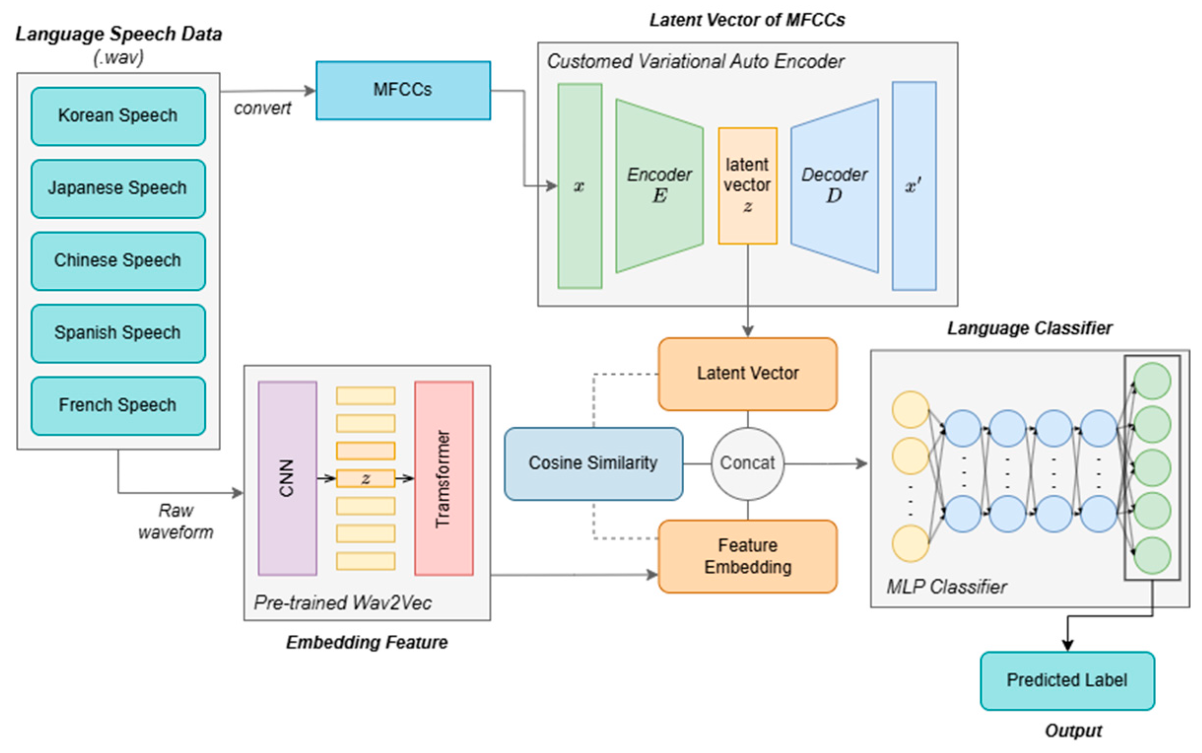
The outputs from the Wav2Vec and VAE encoders were concatenated to form a unified representation. This fusion allows the model to leverage the strengths of both global and local features: pretrained contextual information from Wav2Vec and task-specific latent representations from the VAE. By combining them, the model can better capture the full range of acoustic variability relevant to language identity, leading to improved classification performance. The model overview is illustrated in Figure 2.

3.1. Wav2Vec 2.0

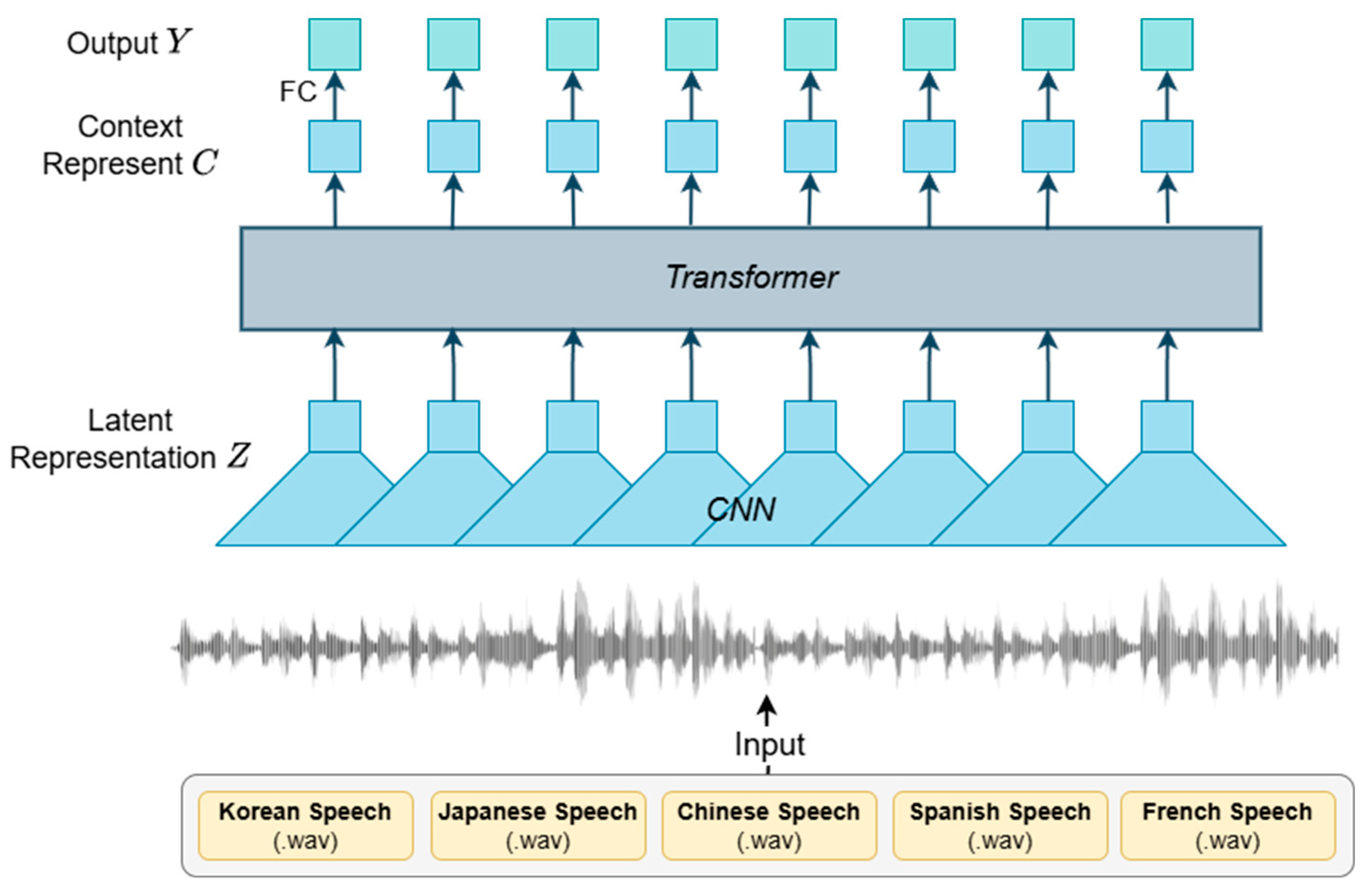
Wav2Vec is a model designed to efficiently learn and encode raw speech signals into fixed-length embeddings for downstream tasks such as speech recognition and language understanding [18]. The architecture comprises three main components: a feature encoder, a Transformer network, and a quantization module. Wav2Vec directly processes raw waveform inputs, enabling it to learn meaningful speech representations even under limited labeled data conditions.

As illustrated in Figure 3, the model employs a Transformer-based structure that operates on framed segments of the input audio. During training, certain frames are masked to encourage the model to learn contextual representations of the speech signal. The convolutional neural network (CNN)-based feature encoder first converts raw audio into low-dimensional feature vectors, while the Transformer’s self-attention mechanism captures temporal dependencies across frames. A contrastive loss objective is utilized to suppress noise and uncertainty, thereby preserving salient speech information.

Figure 4 shows the t-SNE results for the Wav2Vec and VAE embeddings, each visualized separately for train and test sets. All embeddings are 128-dimensional and reduced to 2D using t-SNE for visualization. Although some overlap appears between languages, especially in the Wav2Vec embeddings, this is partly due to the dimensionality reduction and does not necessarily reflect poor separability in the original space.

The VAE vectors show relatively clearer clustering by language, while Wav2Vec embeddings capture broader contextual patterns. The two modules each capture different aspects of the audio: Wav2Vec focuses on high-level phonetic structure, and VAE encodes low-level acoustic features. By combining the two, the model benefits from both representations, which helps improve classification performance.

3.2. Variational Auto Encoder

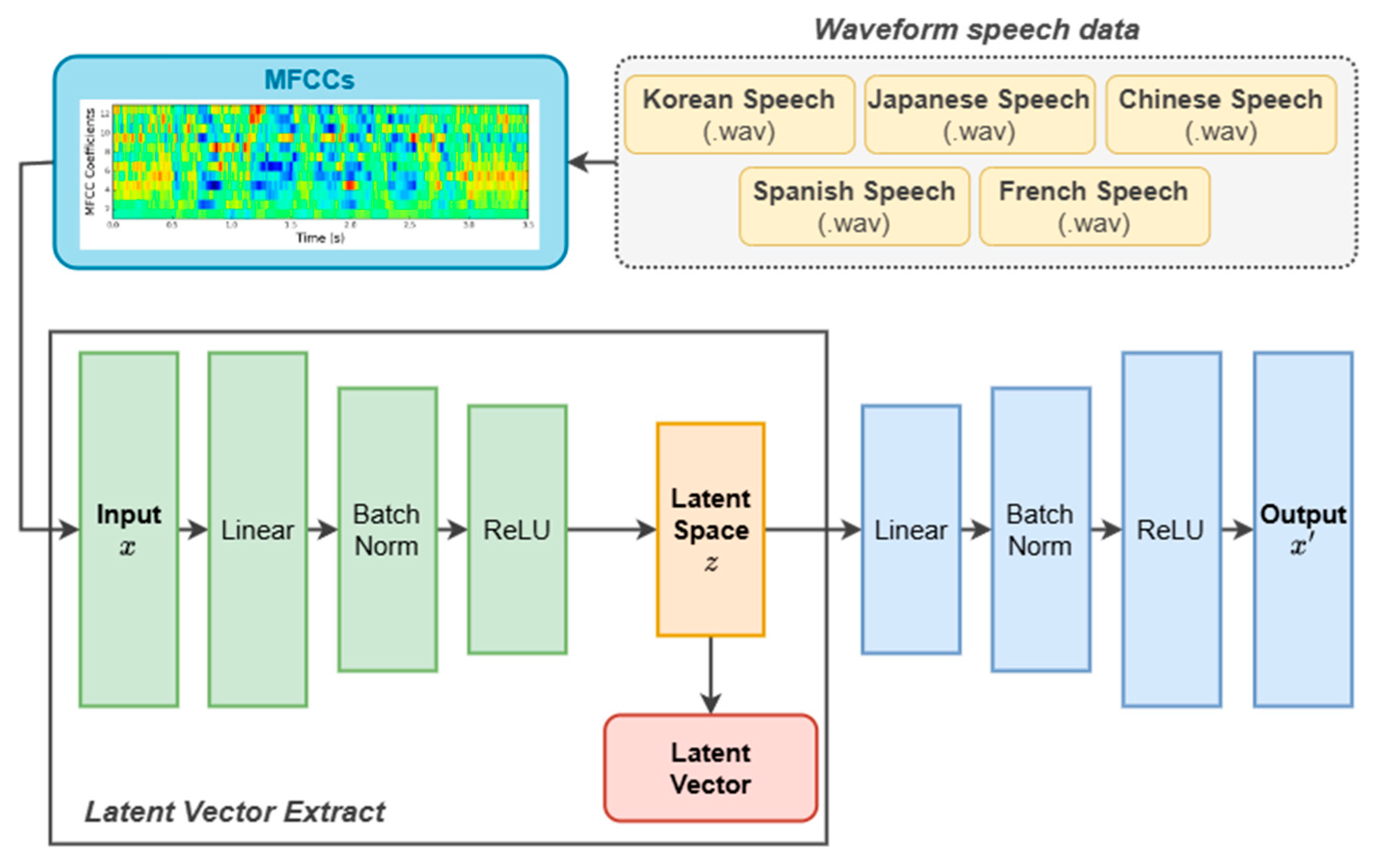
To enhance language classification performance, we incorporated an additional feature extraction process alongside the embeddings obtained from Wav2Vec. Specifically, we developed and trained a VAE [19] model to perform complementary vectorization of speech data as shown in Figure 5. Following end-to-end training, only the encoder component of the VAE is utilized to extract latent representations. These latent vectors serve as auxiliary inputs to the final classifier, contributing to improved discriminative capability.

The VAE was chosen for its ability to utilize the probabilistic distribution of latent space, rather than simply employing a single latent vector. This characteristic allows for a more robust and nuanced representation of the data. Also, it was chosen for its capacity to model complex speech characteristics, such as speaker-specific tone, intonation, and pronunciation variations, which are critical for accurate language identification solely from speech signals. By inputting MFCC features into the VAE, the generative nature of the model facilitates more precise and robust vectorization per language label, extending beyond the mere feature compression of conventional autoencoders. Furthermore, given that the dataset comprises speech samples from different speakers for each language, the VAE’s inherent regularization promotes generalization across speaker variability within the same language class, making it particularly suitable for this task.

For training the autoencoder (AE) [20], input speech signals are first transformed into acoustic feature representations that effectively encapsulate relevant speech characteristics. In this study, MFCCs, which are widely recognized for their effectiveness in capturing phonetic and vocal properties, are extracted and used as input features for the VAE. The Mel scale is derived based on the human cochlea’s auditory system, which exhibits greater frequency resolution at lower frequencies and diminished sensitivity at higher frequencies. Mel-spectrograms provide a time–frequency representation of speech signals mapped onto this perceptually motivated scale. Subsequently, a DCT is applied to the Mel-spectrogram to obtain MFCCs, producing a compact feature vector that retains salient spectral information. Due to their proven capability in representing pronunciation quality and phonetic content, MFCCs are extensively employed in speech recognition and related speech processing applications.

3.3. Classifier Model

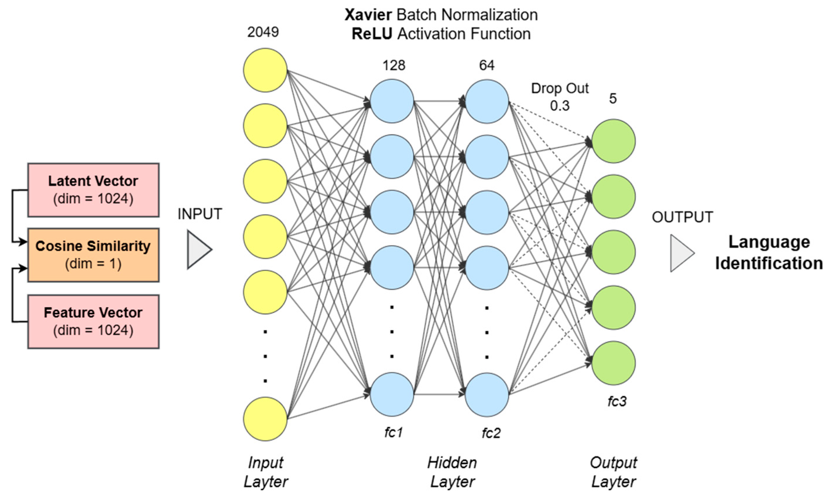
The final language identification model, as shown in Figure 6, was designed as an MLP [21] comprising an input layer, two hidden layers, and an output layer corresponding to the number of target classes. Considering that the input consists of structured high-dimensional vectors and the necessity to learn nonlinear relationships among features, an MLP architecture was adopted. The model employs fully connected (FC) layers to incorporate all input dimensions during training, enabling effective learning of complex patterns.

To mitigate overfitting, Dropout and Batch Normalization layers were incorporated [22]. Dropout was applied with a rate of 0.3 immediately before the output layer to prevent the model from over-relying on specific features. Batch Normalization was utilized to stabilize and accelerate training by normalizing layer inputs; it was initialized based on Xavier initialization [23] to alleviate gradient vanishing and exploding issues during early training stages.

The classifier input comprises three vectors in total. First, the vector generated from speech data via the Wav2Vec model is loaded and converted into a float32 tensor. Second, the latent vector extracted from the VAE is passed through a linear layer to map its dimensionality from 16 to 1024, matching the dimensionality of the Wav2Vec feature vector.

In addition to the vectors extracted from Wav2Vec and VAE, the cosine similarity between these two vectors [24] is computed and included as an additional input feature. Cosine similarity measures the directional similarity between the two vectors, enabling the model to learn patterns corresponding to varying degrees of correlation. This approach facilitates an understanding of how related the feature vectors are, which improves classification by capturing both agreement and divergence patterns between the representations.

These two vectors originate from different models with distinct extraction processes and representation formats. The Wav2Vec model operates directly on raw audio waveforms to generate embeddings, whereas the VAE model first transforms the speech data into MFCCs before encoding them into latent vectors. Due to these inherent differences, simple concatenation of the two vectors may not effectively capture their relationship. Therefore, incorporating their similarity via cosine similarity was deemed a more suitable strategy to enhance the feature representation for the final classifier.

4. Evaluation

4.1. Dataset Preprocessing

The dataset was constructed using spoken utterance data in five languages: Korean, Japanese, Chinese, Spanish, and French. The number of samples per language varies significantly, with 12,854 samples for Korean [25], 9013 for Japanese [26], 3914 for Chinese [27], 14,713 for Spanish [28], and 12,061 for French [29]. All datasets were sourced from publicly available speech corpora on Kaggle, consisting of speaker utterances in response to specific prompts, provided in WAV format.

Notably, the Chinese subset is considerably smaller than the others, raising concerns about data imbalance. To address this issue and improve model generalization, we applied several data augmentation techniques. Specifically, speed perturbation (varying playback speed), volume perturbation (modifying amplitude), and reverberation (simulating real-world acoustic environments) [30] were employed to further diversify the acoustic characteristics of the training data. As a result, an additional 7000 augmented training samples were generated, increasing the total number of Chinese speech samples to 10,914 in the final dataset.

In order to extract meaningful acoustic features for model training, all audio samples were preprocessed using the MFCC technique. MFCCs effectively capture the spectral characteristics of speech signals in a manner that aligns with human auditory perception. Each waveform was transformed into a sequence of MFCC feature vectors through standard signal processing steps including framing, windowing, short-time Fourier transform, and Mel-scale filtering. These MFCC features served as the input representations for the VAE model.

The language-specific speech dataset consisted of a total of 52,555 utterances, which were divided into training, validation, and test sets using an 80:20 split for training and testing, with 20% of the training set further allocated for validation. Additionally, 100 noise samples were incorporated into each language set to enhance the model’s robustness against background noise. The final distribution is shown in

Table 2. Language-specific speech dataset.

	Language-Specific Speech Dataset (.wav, .npy)
	Train	Validation	Test	Total
Korean	8227	2056	2571	12,854
Japanese	5248	1311	2454	9013
Chinese	7279	2569	1066	10,914
Spanish	8552	2138	4023	14,713
French	7141	1785	3135	12,061
Noise Data	100
Mixed Total	36,447	9859	13,249	59,555

.

The noise dataset was sourced from AI Hub [31] Living Environment Noise AI Learning Data [32], which includes 38 types of noise categorized into four groups: interfloor noise, construction noise, business noise, and traffic noise. From this dataset, 100 samples were selected, specifically consisting of traffic and engine noise. These noise samples were then randomly mixed into the speech datasets.

4.2. Training Parameters

Training parameters play a critical role in the performance and convergence of a model [33]. Key parameters such as the learning rate, batch size, and number of epochs significantly affect whether the model is properly trained and capable of generalizing to unseen data. Improper parameter selection may lead to underfitting, overfitting, or unstable training dynamics. Therefore, careful tuning of training parameters is essential to achieve optimal model accuracy and efficiency.

Therefore, the training parameters used in both the VAE and the MLP-based classifier are critical to the overall training process. In the case of the VAE, proper tuning of parameters such as the learning rate and batch size ensures stable optimization and effective latent space representation [34]. For the MLP classifier, these parameters influence the model’s ability to learn discriminative features and generalize well to unseen data [35]. In both cases, careful adjustment of training settings is essential to prevent overfitting, ensure convergence, and maximize classification accuracy.

4.2.1. VAE Training Parameters

To facilitate effective learning in the latent space, the final loss function was defined as a combination of a reconstructive loss based on Binary Cross-Entropy (BCE) [36] and a Kullback–Leibler (KL) divergence loss [37]. The weight of the KL divergence term (β) was set to 0.5, as detailed in

Table 3. VAE training parameters.

VAE Training Parameters
Epoch	30	Weight Initialization	He Initialization
Batch Size	32	Loss Weight	β	0.5
Reconstructive Loss	Binary Cross-Entropy	Divergence Loss	KL Divergence Loss

.

The β value was selected empirically based on preliminary experiments. Lower values (e.g., β = 0.1) tended to produce overly flexible latent distributions, resulting in unstable representations that degraded downstream classification performance. Conversely, larger β values (e.g., β ≥ 1.0) excessively constrained the latent space, leading to underfitting and loss of expressive features. A mid-range value of β = 0.5 offered the best trade-off between latent regularization and representational capacity, and resulted in improved classification accuracy and stability [38].

He initialization [39] was employed to mitigate the issues of vanishing and exploding gradients by appropriately setting the initial weights, thereby enhancing training efficiency. During training, it was observed that the loss values stabilized around epoch 20, exhibiting minimal fluctuations thereafter. Based on this observation, a batch size of 32 was used, and training was conducted for a total of 30 epochs. The training curve depicted in Figure 7 clearly illustrates the negligible changes in loss values beyond epoch 20.

4.2.2. Classifier Training Parameters

When the number of samples for a specific label is significantly lower than that of other classes, the model may become biased towards labels with larger sample sizes. Since the dataset used in this study exhibits class imbalance, we employed K-fold cross-validation [40] and Focal Loss [41] to mitigate this issue during training.

K-fold cross-validation partitions the dataset into multiple subsets, enabling the model to be trained and evaluated across different folds. This approach effectively prevents overfitting by alternately using each fold as a validation set while training on the remaining folds. In this study, the data were divided into five equal folds, facilitating balanced training and validation across classes and helping to alleviate the class imbalance problem.

Focal Loss adjusts the standard cross-entropy loss by applying a modulating factor that emphasizes harder-to-classify samples, thereby assigning higher weights to less frequent labels. This enables the model to reduce the contribution of well-classified (easy) samples and focus learning on more challenging examples. The parameter α in Focal Loss was dynamically set based on the label distribution within each fold during K-fold training, as detailed in

Table 4. Focal Loss weights per K-fold.

Focal Loss α
	Chinese	French	Japanese	Korean	Spanish
K = 1~5	0.431	0.147	0.187	0.119	0.114

. The focusing parameter γ was fixed at 2 to further concentrate learning on minority classes. The loss value for each sample is adjusted accordingly, increasing for difficult samples and decreasing for easy ones. The final loss is computed as the average of these adjusted sample losses.

A learning rate scheduler was also employed to reduce the learning rate at regular epoch intervals. Initially, a relatively high learning rate (2 × 10⁻⁵) was used to enable rapid convergence, followed by gradual reductions to facilitate fine-tuning. The scheduler decreased the learning rate by a factor of 0.5 every 10 epochs, with a step size of 10, helping to prevent overfitting and to more stably approach the loss function’s minimum as shown in

Table 5. Classifier train parameters.

Classifier Train Parameters
Epoch	50		Weight Initialization	Xavier
Batch Size	64		Optimizer	Adam
K-Folds	5		Learning Rate	2 × 10−5
Drop Out	0.3		Batch Normalization	Xavier
Scheduler	stepLR		Loss	Cross-Entropy
	Υ	0.5	Focal Loss	α	Alter
	step	10		Υ	2

. As shown in the fold-wise training curves in Figure 7, while a temporary spike in loss and decrease in accuracy was observed in fold 2, the training process remained generally stable across other folds.

4.3. Performance Evaluation

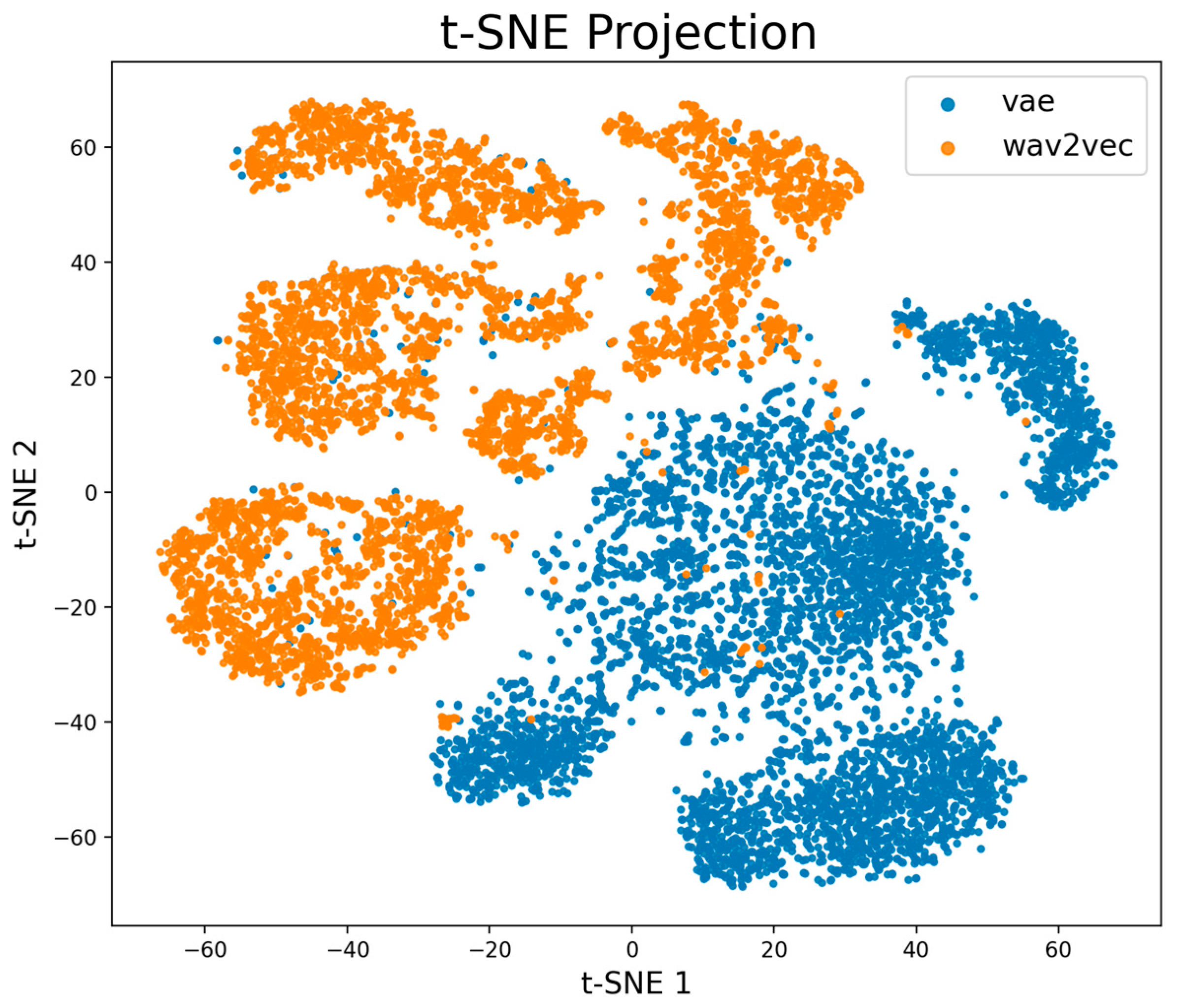
Figure 8 presents the t-SNE projection results for VAE and Wav2Vec embeddings, each reduced from their original 128-dimensional space to two dimensions for visualization. The projection was computed with a mean σ of 0.033, yielding a KL divergence of 84.64 after 250 iterations with early exaggeration and converging to 1.93 after 1000 iterations. As shown, the two embedding types form distinct, well-separated clusters, with minimal overlap between VAE and Wav2Vec representations. This separation suggests that each embedding space captures unique feature distributions, indicating complementary representational properties.

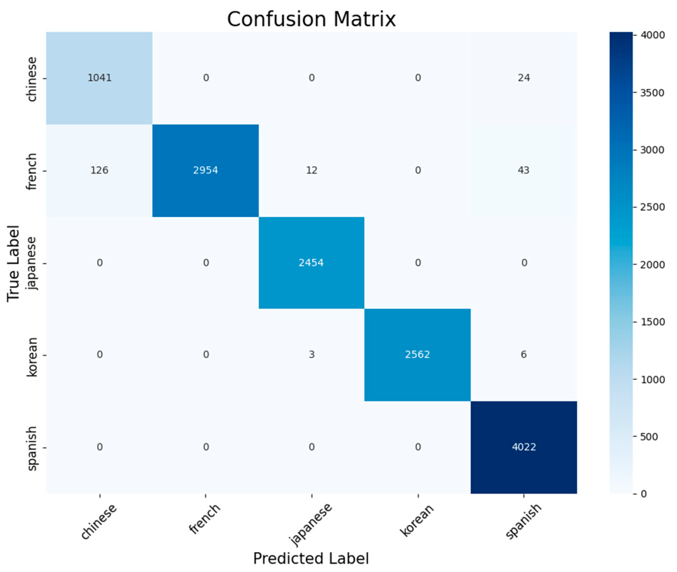
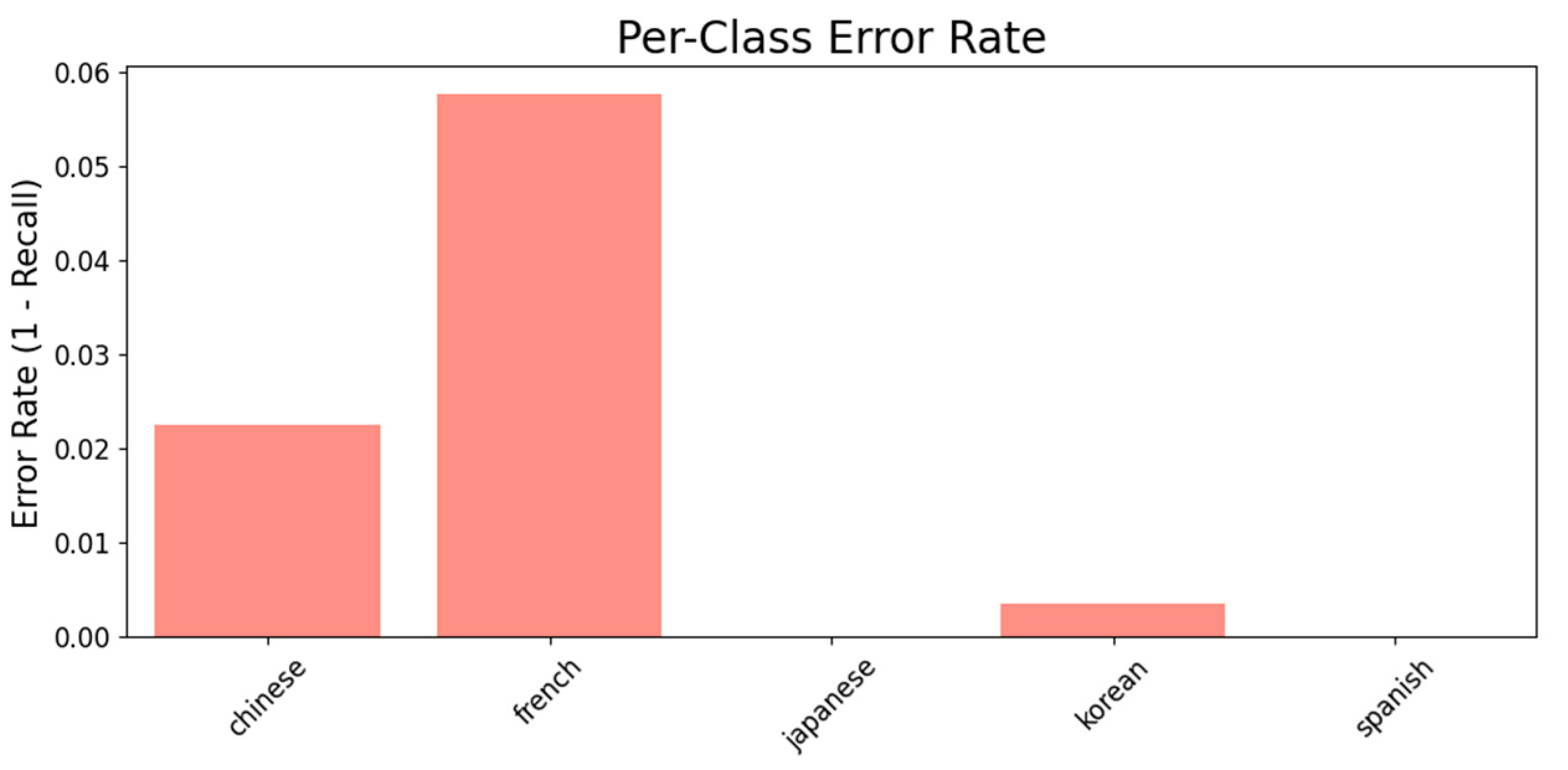
The final model achieved a loss of 0.1063 and an accuracy of 98.38% on the test set, demonstrating overall strong performance in language classification. The confusion matrix indicates that the model performs with high accuracy across most language classes, particularly for Japanese, Korean, and Spanish, each showing minimal or no confusion with other classes. Figure 9 presents the confusion matrix of the model, illustrating its performance across different classes. Complementing this, Figure 10 displays the per-class error rate, providing a detailed breakdown of misclassifications for each individual class.

However, the French class exhibited the most frequent misclassifications. Out of a total of 3135 French samples, 126 were incorrectly classified as Chinese, 12 as Japanese, and 43 as Spanish, suggesting that the model occasionally confuses French with phonetically or acoustically similar languages. This may be due to shared phonetic patterns between French and these languages in certain acoustic contexts.

Meanwhile, Chinese had a minor confusion with Spanish (24 instances), and Korean showed only 9 misclassifications in total (3 as Japanese, 6 as Spanish), further supporting the robustness of the classifier for these languages.

Overall, the confusion matrix highlights strong class separability, with the few misclassifications largely concentrated in language pairs that may share overlapping acoustic features. These insights could guide future work on enhancing the model’s discriminative power, especially for closely related or phonetically ambiguous language pairs.

The per-class error rate plot further supports the findings from the confusion matrix by quantifying the misclassification rate for each language class. Notably, the French class exhibits the highest error rate, exceeding 5.5%, which aligns with the previously observed confusion with Chinese and Spanish samples. The Chinese class also shows a moderate error rate of approximately 2.2%, primarily due to misclassifications as Spanish. In contrast, Japanese and Spanish classes demonstrate perfect or near-perfect recall, indicating zero or negligible misclassifications. The Korean class shows a minimal error rate below 0.5%, affirming the model’s strong ability to distinguish Korean from other languages. These results highlight the model’s robustness across most classes, while also identifying French as a challenging category.

The classification report in

Table 6. Language classification report over 50 test runs.

Language Classification Report
	Precision	Recall	F1-Score	Std. Dev.
Korean	1.00	1.00	1.00	0.00
Japanese	0.99	1.00	1.00	0.00
Chinese	0.89	0.98	0.93	0.00
Spanish	0.98	1.00	0.99	0.00
French	1.00	0.94	0.93	0.00
Total Accuracy	98.38%

provides detailed per-class evaluation metrics that reinforce the observations from the confusion matrix and the per-class error rate plot. To assess the statistical reliability of these results, the evaluation was conducted over 50 independent test runs, each initialized with a different random seed. For each run, precision, recall, and F1-score were computed per class, and their mean values and standard deviations were reported. Across all metrics and classes, the standard deviations were found to be negligible (less than 0.001), indicating highly stable and reproducible classification performance across different initializations.

The model achieves perfect precision and recall (1.00) for both Korean and Japanese, resulting in flawless F1-scores of 1.00, which demonstrates exceptional discriminative capability for these languages. Spanish also shows consistently high performance, with a precision of 0.98, recall of 1.00, and F1-score of 0.99, suggesting minimal false negatives and strong overall classification.

The Chinese class yields a slightly lower precision of 0.89 while maintaining a high recall of 0.98, which indicates that while most Chinese samples are correctly identified, some samples from other languages are mistakenly classified as Chinese, leading to a higher false positive rate.

The French class presents the most noticeable drop in performance, with a recall of 0.94, despite a perfect precision of 1.00. This suggests that while all samples predicted as French are indeed correct, the model fails to identify approximately 6% of actual French samples, often misclassifying them as Chinese or Spanish. This aligns precisely with the error distribution observed earlier.

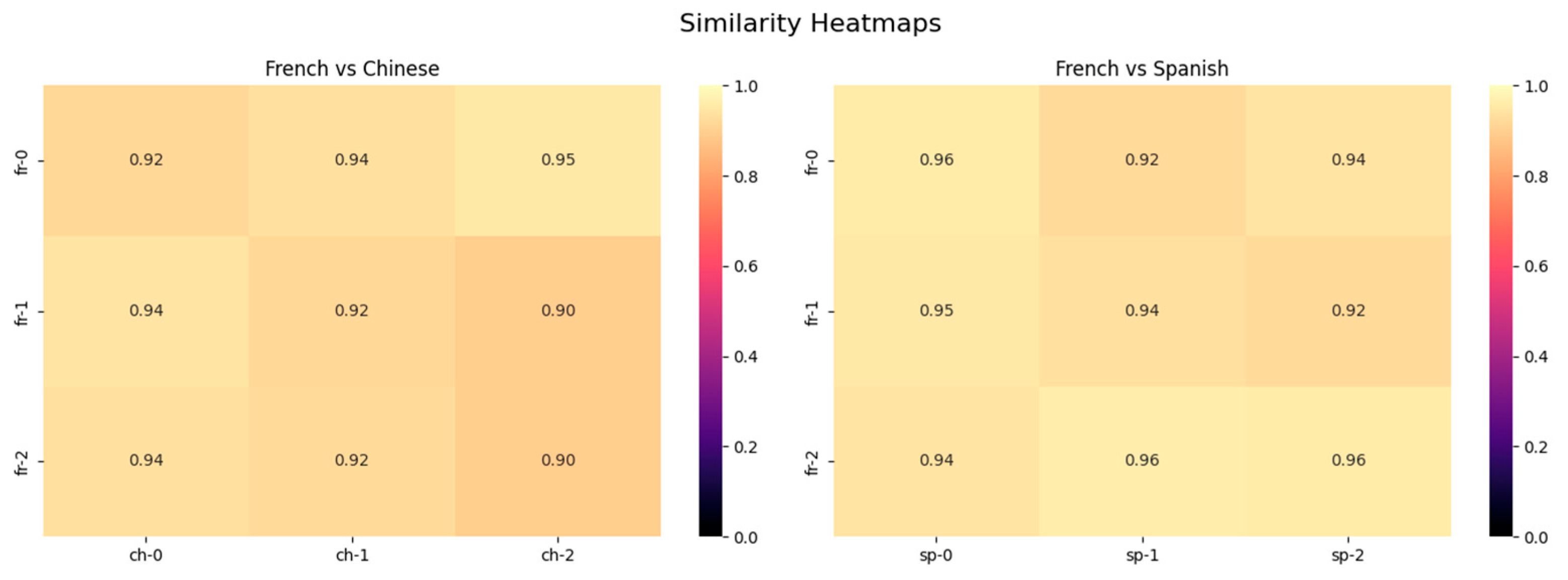
These misclassification patterns can be further understood by examining the acoustic similarities between the languages. French and Spanish both belong to the Romance language family and share similar phonetic structures, including consonant-vowel ratios, phoneme durations, and prosodic characteristics [42]. French is particularly notable for its nasalization and fluid phoneme transitions, while Spanish tends to exhibit clearer syllable boundaries. Mandarin Chinese, although distinct as a tonal language, demonstrates phonetic overlap with French in non-tonal regions [43]. MFCC similarity heatmaps shown in Figure 11 further confirm these overlaps, with French–Chinese and French–Spanish pairs exhibiting high similarity scores ranging from 0.90 to 0.96. These findings indicate that the model perceives both language pairs as acoustically similar in the MFCC domain, contributing to the observed classification confusions.

The model’s overall accuracy of 98.38% confirms strong global performance, with high consistency across most language classes. However, the imbalance in precision and recall for certain classes (particularly French and Chinese) indicates specific areas for further refinement, possibly by incorporating more robust feature representations or addressing phonetic overlap between confusing pairs.

To evaluate the feasibility of deploying the proposed lightweight classifier in real-world embedded scenarios, we conducted a profiling analysis measuring key performance metrics including computational cost, inference latency, and memory consumption. The classifier requires approximately 0.27 MFLOPs per input and achieves an average inference time of 0.344 ms per sample on an NVIDIA RTX 8000 GPU. The peak memory usage is limited to 11.47 MB, indicating that the model is highly efficient in terms of both computation and memory footprint.

To assess the practical deployment potential, we compared expected inference performance across two widely used edge devices: Raspberry Pi 5 and Jetson Nano. Based on known hardware capabilities and extrapolated benchmarking data, the Jetson Nano is estimated to perform inference at approximately 2–3 FPS with moderate latency, whereas the Raspberry Pi 5 would likely achieve 1–2 FPS, subject to thermal constraints and CPU-only execution. A detailed comparison is provided in

Table 7. Edge device inference performance comparison.

	RTX 8000	Raspberry Pi 5	Jetson Nano	Jetson Nano with TensorRT
Flops Per Sample	0.27 MFLOPs	0.27 MFLOPs	0.27 MFLOPs	0.19 MFLOPs
Average Inference Time	0.344 ms	15 ms	5 ms	3.5 ms
Peak Memory Usage	11.47 MB	15 MB	12 MB	9 MB

.

These results demonstrate that the proposed model is suitable for resource-constrained environments where real-time or near real-time performance is required. In contrast to heavy-weight transformer-based or multi-stream architectures, our model offers a highly deployable alternative for practical LID applications without sacrificing classification accuracy.

We implemented a prototype on the NVIDIA Jetson Nano, a compact embedded computing platform that is widely adopted in mobility-oriented hardware systems. The Jetson Nano was selected because hardware configurations in mobility devices are often highly heterogeneous, making it difficult to standardize deployment targets. The model was first trained on an RTX 8000 GPU, after which the trained model files were converted to TensorRT format and deployed to the Jetson Nano. This conversion not only ensured compatibility but also typically yielded improved inference performance as shown in Table 7.

To validate the deployment, we conducted real-time tests on the Jetson Nano with and without TensorRT optimization, observing that the TensorRT version generally achieved better performance. The evaluation involved a test group of 20 participants (10 male and 10 female), ranging in age from their teens to their fifties, all of whom were capable of speaking at least two languages. Each participant was tested in multiple languages, and the results were analyzed on a per-language basis. The prototype achieved an overall accuracy of approximately 96% in this embedded setting, while maintaining real-time responsiveness.

Table 8. Language classification and resource comparison.

Language Classification Model Comparison Report
	CNN [44]	Whisper [45]	Speechbrain [46]	Our Model
Korean (F1)	0.50	0.99	0.99	1.00
Japanese (F1)	0.98	0.99	0.99	1.00
Chinese (F1)	0.96	1.00	0.99	0.93
Spanish (F1)	0.67	0.99	0.26	0.99
French (F1)	0.73	0.99	0.96	0.93
Memory Usage	90.58 MB	2989.86 MB	191.84 MB	11.47 MB
Average Inference Time	0.5505 s	0.1935 s	0.0884 s	0.344 ms

presents a comparative analysis between the proposed model, a traditional CNN baseline [44], and two representative state-of-the-art language identification systems, Whisper [45] and Speechbrain [46], in terms of F1-score, memory usage, and inference speed. The CNN baseline records the lowest overall performance, with marked drops for Korean (0.50) and Spanish (0.67). Whisper attains the highest or near-highest F1-scores for all five languages, but its memory footprint approaches 3 GB, which limits applicability in embedded or mobile environments. Speechbrain performs consistently well for most languages but shows a pronounced weakness in Spanish (0.26), reflecting reduced robustness for that category.

In contrast, the proposed model sustains high F1-scores across all languages achieving 1.00 for Korean and Japanese, 0.99 for Spanish, and competitive scores for Chinese and French, while requiring only 11.47 MB of memory and delivering an inference time of 0.344 ms. This combination of strong accuracy, low resource usage, and fast processing makes it an effective choice for real-time multilingual speech recognition, especially where both high performance and computational efficiency are essential.

5. Conclusions

Addressing the observed imbalances in precision and recall for French and Chinese classes is paramount. Future work will explore several avenues, including the incorporation of more robust and discriminative acoustic feature representations to better capture the subtle phonetic nuances between confusing language pairs. Furthermore, investigating advanced techniques to mitigate misclassification, such as implementing data augmentation strategies specifically designed to enrich the representation of challenging languages like French and Chinese, could significantly enhance the model’s performance in these categories. In addition, future research will include a comprehensive performance comparison with state-of-the-art LID models to further assess the strengths and limitations of the proposed approach. Ultimately, these efforts aim to develop an even more robust and universally accurate language identification system.

References

1. Available online: https://papago.naver.com/ (accessed on 1 August 2025).
2. Available online: https://translate.google.co.kr/ (accessed on 1 August 2025).
3. Zissman, M.A. Comparison of four approaches to automatic language identification of telephone speech. IEEE Trans. Speech Audio Process. 1996, 4, 31. [Google Scholar] [CrossRef]
4. Manchala, S.; Kamakshi Prasad, V.; Janaki, V. GMM based language identification system using robust features. Int. J. Speech Technol. 2014, 17, 99–105. [Google Scholar] [CrossRef]
5. Yan, Y.; Barnard, E. An approach to automatic language identification based on language-dependent phone recognition. In Proceedings of the 1995 International Conference on Acoustics, Speech, and Signal Processing, Detroit, MI, USA, 9–12 May 1995; IEEE: New York, NY, USA, 1995; Volume 5, pp. 3511–3514. [Google Scholar]
6. Zissman, M.A.; Singer, E. Automatic language identification of telephone speech messages using phoneme recognition and n-gram modeling. In Proceedings of the ICASSP’94. IEEE International Conference on Acoustics, Speech and Signal Processing, Adelaide, SA, Australia, 19–22 April 1994; IEEE: New York, NY, USA, 1994; Volume 1, pp. 1–305. [Google Scholar]
7. Gauvain, J.L.; Messaoudi, A.; Schwenk, H. Language recognition using phone latices. In Proceedings of the INTERSPEECH, Jeju, Republic of Korea, 4–8 October 2004; pp. 25–28. [Google Scholar]
8. Zhang, X.; Trmal, J.; Povey, D.; Khudanpur, S. Improving deep neural network acoustic models using generalized maxout networks. In Proceedings of the 2014 IEEE International Conference on Acoustics, Speech and Signal Processing (ICASSP), Florence, Italy, 4–9 May 2014; IEEE: New York, NY, USA, 2014; pp. 215–219. [Google Scholar]
9. Lopez-Moreno, I.; Gonzalez-Dominguez, J.; Plchot, O.; Martinez, D.; Gonzalez-Rodriguez, J.; Moreno, P. Automatic language identification using deep neural networks. In Proceedings of the 2014 IEEE International Conference on Acoustics, Speech and Signal Processing (ICASSP), Florence, Italy, 4–9 May 2014; IEEE: New York, NY, USA, 2014; pp. 5337–5341. [Google Scholar]
10. Available online: https://catalog.ldc.upenn.edu/LDC2014S06 (accessed on 1 August 2025).
11. Available online: https://www.kaggle.com/datasets/zarajamshaid/language-identification-datasst (accessed on 1 August 2025).
12. Dave, N. Feature extraction methods LPC, PLP and MFCC in speech recognition. Int. J. Adv. Res. Eng. Technol. 2013, 1, 1–4. [Google Scholar]
13. Gupta, S.; Jaafar, J.; Ahmad, W.W.; Bansal, A. Feature extraction using MFCC. Signal Image Process. Int. J. 2013, 4, 101–108. [Google Scholar] [CrossRef]
14. Hönig, F.; Stemmer, G.; Hacker, C.; Brugnara, F. Revising Perceptual Linear Prediction (PLP). In Proceedings of the INTERSPEECH, Lisbon, Portugal, 4–8 September 2005; pp. 2997–3000. [Google Scholar]
15. Gupta, H.; Gupta, D. LPC and LPCC method of feature extraction in Speech Recognition System. In Proceedings of the 2016 6th International Conference-Cloud System and Big Data Engineering (Confluence), Noida, India, 14–15 January 2016; IEEE: New York, NY, USA, 2016; pp. 498–502. [Google Scholar]
16. Wang, Y.; Yang, Y.; Yuan, J. Normalization through Fine-tuning: Understanding Wav2vec 2.0 Embeddings for Phonetic Analysis. arXiv 2025, arXiv:2503.04814. [Google Scholar]
17. Latif, S.; Rana, R.; Qadir, J.; Epps, J. Variational autoencoders for learning latent representations of speech emotion: A preliminary study. arXiv 2017, arXiv:1712.08708. [Google Scholar]
18. Baevski, A.; Zhou, Y.; Mohamed, A.; Auli, M. wav2vec 2.0: A framework for self-supervised learning of speech representations. In Proceedings of the Advances in Neural Information Processing Systems, Online, 6–12 December 2020; Volume 33, pp. 12449–12460. [Google Scholar]
19. Kingma, D.P.; Welling, M. Auto-Encoding Variational Bayes. Available online: https://pure.uva.nl/ws/files/2511146/162970_1312.6114v10.pd.pdf (accessed on 1 August 2025).
20. Bank, D.; Koenigstein, N.; Giryes, R. Autoencoders. In Machine Learning for Data Science Handbook: Data Mining and Knowledge Discovery Handbook; Springer: Cham, Switzerland, 2023; pp. 353–374. [Google Scholar]
21. Popescu, M.C.; Balas, V.E.; Perescu-Popescu, L.; Mastorakis, N. Multilayer perceptron and neural networks. WSEAS Trans. Circuits Syst. 2009, 8, 579–588. [Google Scholar]
22. Ying, X. An overview of overfitting and its solutions. J. Phys. Conf. Ser. 2019, 1168, 022022. [Google Scholar] [CrossRef]
23. Kumar, S.K. On weight initialization in deep neural networks. arXiv 2017, arXiv:1704.08863. [Google Scholar] [CrossRef]
24. Lahitani, A.R.; Permanasari, A.E.; Setiawan, N.A. Cosine similarity to determine similarity measure: Study case in online essay asessment. In Proceedings of the 2016 4th International Conference on Cyber and IT Service Manage-Ment, Bandung, Indonesia, 26–27 April 2016; IEEE: New York, NY, USA, 2016; pp. 1–6. [Google Scholar]
25. Available online: https://www.kaggle.com/datasets/bryanpark/korean-single-speaker-speech-dataset (accessed on 1 August 2025).
26. Available online: https://www.kaggle.com/datasets/bryanpark/japanese-single-speaker-speech-dataset (accessed on 1 August 2025).
27. Available online: https://www.kaggle.com/datasets/bryanpark/chinese-single-speaker-speech-dataset (accessed on 1 August 2025).
28. Available online: https://www.kaggle.com/datasets/bryanpark/spanish-single-speaker-speech-dataset (accessed on 1 August 2025).
29. Available online: https://www.kaggle.com/datasets/bryanpark/french-single-speaker-speech-dataset (accessed on 1 August 2025).
30. Cui, X.; Goel, V.; Kingsbury, B. Data augmentation for deep neural network acoustic modeling. IEEE/ACM Trans. Audio Speech Lang. Process. 2015, 23, 1469–1477. [Google Scholar]
31. Available online: https://www.aihub.or.kr/ (accessed on 1 August 2025).
32. Available online: https://www.aihub.or.kr/aihubdata/data/view.do?currMenu=115&topMenu=100&dataSetSn=71296 (accessed on 1 August 2025).
33. Akinlolu Ilemobayo, J.; Durodola, O.; Alade, O.; Awotunde, O.J.; Olanrewaju, A.T.; Falana, O.; Ogungbire, A.; Osinuga, A.; Ogunbiyi, D.; Odezuligbo, I.; et al. Hyperparameter tuning in machine learning: A comprehensive review. J. Eng. Res. Rep. 2024, 26, 388–395. [Google Scholar] [CrossRef]
34. Rybkin, O.; Daniilidis, K.; Levine, S. Simple and effective VAE training with calibrated decoders. In Proceedings of the International Conference on Machine Learning, Virtual, 18–24 July 2021; pp. 9179–9189. [Google Scholar]
35. El-Hassani, F.Z.; Amri, M.; Joudar, N.E.; Haddouch, K. A new optimization model for MLP hyperparameter tuning: Modeling and reso-lution by real-coded genetic algorithm. Neural Process. Lett. 2024, 56, 105. [Google Scholar] [CrossRef]
36. Ho, Y.; Wookey, S. The real-world-weight cross-entropy loss func-tion: Modeling the costs of mislabeling. IEEE Access 2019, 8, 4806–4813. [Google Scholar] [CrossRef]
37. Kim, T.; Oh, J.; Kim, N.; Cho, S.; Yun, S.Y. Comparing kull-back-leibler divergence and mean squared error loss in knowledge distilla-tion. arXiv 2021, arXiv:2105.08919. [Google Scholar]
38. Bozkurt, A.; Esmaeili, B.; Tristan, J.B.; Brooks, D.; Dy, J.; van de Meent, J.W. Rate-regularization and generalization in variational autoencoders. In Proceedings of the International Conference on Artificial Intelligence and Statistics, Virtual, 13–15 April 2021; pp. 3880–3888, PMLR. [Google Scholar]
39. Datta, L. A survey on activation functions and their relation with xavier and he normal initialization. arXiv 2020, arXiv:2004.06632. [Google Scholar] [CrossRef]
40. Wong, T.T.; Yeh, P.Y. Reliable accuracy estimates from k-fold cross validation. IEEE Trans. Knowl. Data Eng. 2019, 32, 1586–1594. [Google Scholar] [CrossRef]
41. Lin, T.Y.; Goyal, P.; Girshick, R.; He, K.; Dollár, P. Focal loss for dense object detection. In Proceedings of the IEEE International Conference on Computer Vision, Venice, Italy, 22–29 October 2017; pp. 2980–2988. [Google Scholar]
42. Pigoli, D.; Hadjipantelis, P.Z.; Coleman, J.S.; Aston, J.A. The statistical analysis of acoustic phonetic data: Exploring differences between spoken Romance languages. J. R. Stat. Soc. Ser. C Appl. Stat. 2018, 67, 1103–1145. [Google Scholar] [CrossRef]
43. Towfic, Z.J.; Chen, J.; Sayed, A.H. Distributed inference over regression and classification models. In Proceedings of the 2013 IEEE International Conference on Acoustics, Speech and Signal Processing, Vancouver, BC, Canada, 26–31 May 2013; IEEE: New York, NY, USA, 2013; pp. 5406–5410. [Google Scholar]
44. Available online: https://github.com/SpeechFlow-io/Spoken_language_identification (accessed on 1 August 2025).
45. Radford, A.; Kim, J.W.; Xu, T.; Brockman, G.; McLeavey, C.; Sutskever, I. Robust speech recognition via large-scale weak supervision. In Proceedings of the International Conference on Machine Learning, Honolulu, HI, USA, 23–29 July 2023; pp. 28492–28518. [Google Scholar]
46. Available online: https://github.com/speechbrain/speechbrain (accessed on 1 August 2025).
Figure 1. Description of MFCCs, PLP coefficients and LPCCs: (a) extraction process of each speech audio feature; (b) visualization of each speech audio feature.
Applsci 15 09209 g001
Figure 2. Overview of the proposed LID model.
Applsci 15 09209 g002
Figure 3. Architecture of Wav2Vec 2.0 that the proposed LID model employs.
Applsci 15 09209 g003
Figure 4. Visualization of Wav2Vec and VAE latent vector.
Applsci 15 09209 g004
Figure 5. Architecture of Variational Auto Encoder.
Applsci 15 09209 g005
Figure 6. Architecture of Language Identification Model.
Applsci 15 09209 g006
Figure 7. Training curve: (a) classifier training curves per fold; (b) VAE training curve.
Applsci 15 09209 g007
Figure 8. Test result of VAE and Wav2Vec t-SNE projection.
Applsci 15 09209 g008
Figure 9. Test result of confusion matrix.
Applsci 15 09209 g009
Figure 10. Per-class error rate.
Applsci 15 09209 g010
Figure 11. MFCC similarity between French–Chinese and French–Spanish.
Applsci 15 09209 g011