Article

An Efficient and Practical 2D FEM-Based Framework for AC Resistance Modeling of Litz Wire Windings

Department of Electronic Engineering, College of Engineering, Keimyung University, Daegu 42601, Republic of Korea
Appl. Sci. 2025, 15(16), 9185; https://doi.org/10.3390/app15169185
Submission received: 3 June 2025 / Revised: 14 August 2025 / Accepted: 16 August 2025 / Published: 21 August 2025
(This article belongs to the Section Electrical, Electronics and Communications Engineering)

Abstract

Litz wires are extensively employed in contemporary high-frequency switching power electronics to mitigate conductor losses. Minimizing additional winding losses caused by high-frequency phenomena, such as skin and proximity effects, is a critical design consideration for achieving high power density in modern power electronics. However, accurately predicting losses in structures composed of numerous twisted and insulated strands remains a challenge. With the increasing accessibility of commercial numerical tools, such as finite element method (FEM) solvers, simulation-based approaches have become indispensable tools for analyzing electromagnetic phenomena in complex magnetic device structures under high-frequency conditions. In parallel, data-driven modeling has emerged as a powerful method, enabling pattern identification based on datasets; however, such approaches rely on the availability of large amounts of reliable high-quality data. Generating such large-scale FEM datasets, however, is often constrained by long computation times and high memory consumption. Despite the remarkable advancements in computing power, full three-dimensional (3D) FEM analysis at the strand level for Litz wire windings often remains infeasible within personal computing environments. To address these challenges, this study presents a computationally efficient two-dimensional FEM-based framework that integrates a data-driven fitting model with optimized geometric discretization and meshing strategies, enabling accurate analysis with reduced computational load. The proposed approach, which incorporates optimal meshing conditions into commercially available 2D FEM tools and a simple data-driven fitting model, enables accurate prediction of the frequency-dependent AC resistance of multi-turn Litz windings using a typical personal computer. Its feasibility is further demonstrated through experimental frequency response measurements on both 12-turn and 21-turn windings fabricated with 150-strand Litz wire, which show strong agreement with the corrected simulation results, confirming the model’s accuracy and practical applicability.

1. Introduction

Understanding the skin and proximity effects is essential for designing efficient Litz wire windings, particularly in such applications as compact transformers, inductors, wireless power transfer systems, and electromagnetic interference filters used in high-frequency power electronics [1,2,3,4,5]. These frequency-dependent phenomena significantly influence conductor losses and, if not properly addressed, can degrade the performance of high-density power conversion systems. Litz wire, composed of numerous twisted and woven insulated strands, as shown in Figure 1, is a widely adopted solution to mitigate high-frequency losses. However, its complex structure makes analytical modeling of these effects highly challenging.
Early research on the modeling of multi-layer or multi-strand wire windings primarily focused on deriving closed-form analytical expressions by simplifying the geometry to a one-dimensional representation, thereby reducing it to a solvable ordinary differential equation. While this approach yields exact solutions, it inevitably introduces errors due to structural simplifications and idealized boundary conditions [6,7,8,9,10,11,12,13,14]. These theoretical approaches offer valuable insights. Nevertheless, these approaches have limitations when applied to Litz wires consisting of hundreds to thousands of intricately twisted strands. More advanced analytical methods for predicting the AC resistance of Litz wire and determining optimal stranding configurations have been extensively investigated [15,16,17,18]. However, the complexity of the formulations and the large number of parameters may present practical difficulties for engineers in real-world applications.
The widespread accessibility of commercial numerical analysis tools, including FEM, has led to the growing adoption of simulation-based methods in engineering analysis. Although 2D FEM analysis offers clear advantages over 3D FEM, such as significantly lower complexity and reduced computational resources, it cannot represent the twisted geometry of Litz wire characterized by pitch, the axial distance of one rotation. Studies have attempted analytical modeling incorporating this parameter, i.e., pitch [17,18], while some studies actually utilized advanced computational resources to directly analyze pitch effects in 3D geometries [19]. Nevertheless, such approaches may be less applicable for practical engineering environments when access to highly specialized equipment or advanced theoretical expertise is limited.
Notably, the key insight from previous studies is that beyond a certain level of twisting, the Litz wire reaches a condition in which the effective resistance of each strand becomes equal, resulting in shared current among all strands. Although a short pitch increases the overall conductor length and consequently raises DC resistance, it effectively suppresses bundle-level effects. Recent advancements in manufacturing technology have enabled commercially available Litz wires to minimize bundle-level effects through appropriate twisting and weaving patterns. The resulting increase in DC resistance is independent of frequency and can be readily measured in practice. Recent advanced approaches using various numerical methods and equivalent circuit models allow for the representation of transposition patterns in Litz wire without requiring full 3D meshing. Such hybrid methods can serve as a practically viable and accurate alternative for analyzing skin and proximity effects in realistic winding geometries [18,19,20,21,22,23,24,25,26].
This paper presents a 2D FEM-based, data-driven fitting approach that identifies optimal discretization and meshing conditions, thereby delivering high accuracy at substantially lower computational cost as a practical alternative to conventional 3D analysis. By utilizing commercially available ANSYS Electronic Desktop 2024 Maxwell2D on standard personal computers, the proposed workflow generates and analyzes an extensive set of simulation data to derive these optimal settings. This strategy significantly reduces computational complexity without compromising fidelity. Experimental validation on actual multi-turn Litz wire windings confirms the method’s accuracy and applicability in real-world engineering environments.

2. High-Frequency Loss Mechanisms in Conductors

2.1. Frequency-Dependent Loss Mechanisms in Conductors: Skin and Proximity Effects

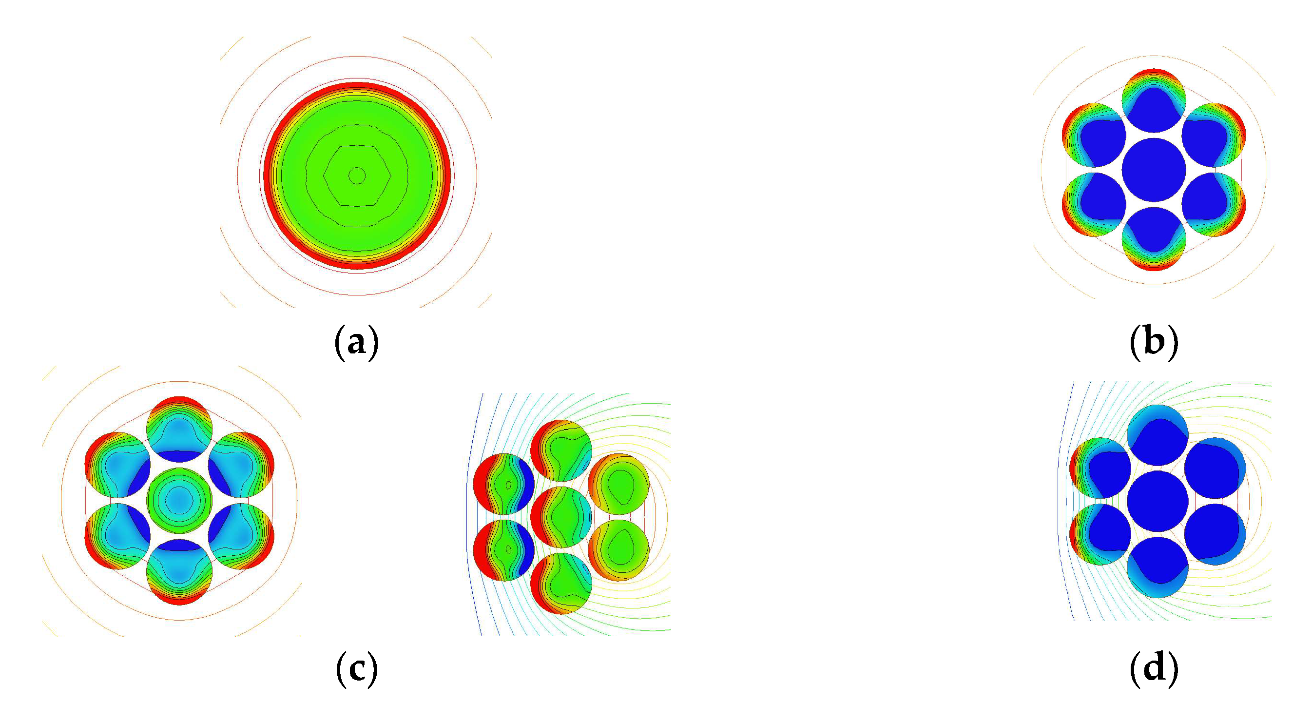
Prior research [12,13] provides a detailed explanation of high-frequency effects in Litz wire, categorizing the primary mechanisms into skin effects and proximity effects at both the strand level and the bundle level in Figure 2. Bundle-level effects are governed by the wire’s overall twist and weave pattern and are largely independent of strand count or diameter. At the strand level, the proximity effect dominates in multi-layer windings, such as Litz wire, which inherently contains a large number of layers, while the skin effect becomes negligible at high frequencies where the wavelength is sufficiently short relative to the conductor cross-sectional area. A tightly twisted pattern with a short pitch effectively attenuates bundle-level effects; however, such construction can lead to an increase in DC resistance. Strand-level proximity effect is influenced by both internal and external fields.
The frequency-dependent conductor loss due to skin and proximity effects in windings is expressed as follows:
P l o s s f = R a c f I 2 = F s k i n f R d c I 2 + F p r o x f | H | 2
where R d c   and   R a c is the resistance under DC conditions and the frequency-dependent AC resistance, respectively, I is the rms value of the current, and H is the peak value of the external magnetic field [7].
The analytical solutions of F s k i n f is well established, and F p r o x f can be approximately calculated in cases where the external field is nearly transverse, such as in tightly aligned wires in highly permeable materials [7,8]. The resulting field distribution depends on various operating conditions, including the cross-sectional area of each strand, the operating frequency, and the pitch of the winding. Selecting the optimal strand size and quantity is a critical design factor for minimizing losses in Litz wires.
In commercial Litz wire products, appropriate twisting effectively prevents bundle-level effects, ensuring the primary purpose of Litz wire is achieved. This simplification holds even if bundle-level skin effect is present, as it is independent of strand count and orthogonal to strand-level losses. Thus, this study focuses on strand-level losses as the primary contributor to high-frequency resistance in Litz wire. These results indicate that the 3D structural variations in Litz wires can be effectively represented using a two-dimensional model through appropriate boundary conditions.

2.2. Analytical Solutions for an Infinitely Long Isolated Conductor

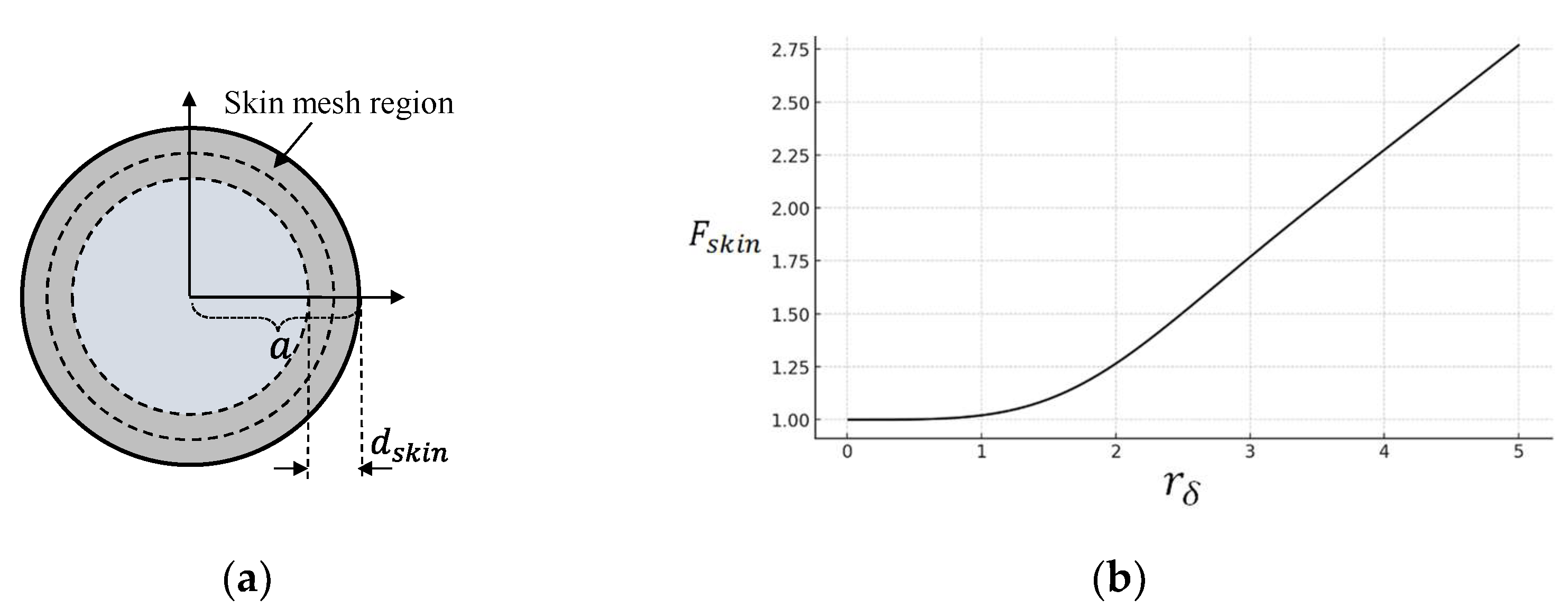
In the case of an infinitely long isolated conductor in Figure 3, the boundary conditions are clearly defined in the absence of external magnetic fields, and a closed-form solution can be derived. Although it holds only under highly constrained conditions, the comparison between FEM results and analytical solutions can serve as a useful benchmark for evaluating the accuracy of simplified models.
The skin depth ( δ ) represents the penetration depth of electromagnetic waves in a conductive material, where the wave’s amplitude decays to 1/e of its original value. For a plane wave incident on a conductive medium, the skin depth in terms of material properties is expressed as follows:
δ = 1 π f μ σ ,
where μ   and   σ are the magnetic permeability and the conductivity, respectively.
To determine the current distribution over the cross-sectional area of an isolated circular conductor, the exact analytical solution of the two-dimensional magnetic diffusion equation in cylindrical coordinates, expressed in phasor form, is as follows:
1 r d d r r d J ^ z d r λ 2 J ^ z ( r ) = 0 ,
where J ^ z ( r ) is the current density in phasor form and λ is 1 + j δ .
Capacitive displacement currents and charge accumulation are neglected. The current density at the center is lower than that at the outer boundary surface. As a note, numerical analysis requires careful consideration of mesh resolution near the conductor surface, the skin mesh region shown in Figure 3a, to ensure accurate computation.
The current density in phasor form is, therefore, expressed as follows:
J ^ z r = I λ 2 π a I 0 λ r I 1 λ a .
where I 0   and   I 1 are modified Bessel functions of the first kinds, respectively.
The internal impedance per unit length Z i n t   is expressed as follows:
Z i n t = λ 2 π a σ I 0 λ a I 1 λ a .  
The F s k i n   of an infinitely long isolated circular conductor is expressed as follows:
F s k i n = R e Z i n t R d c = 1 2 R e 1 + j r δ I 0 1 + j r δ I 1 1 + j r δ .  
In this case, only the strand-level skin effect is present, and, thus, F p r o x = 0 . The F s k i n remains nearly constant at low frequencies and begins to increase at the corner frequency near the skin depth, corresponding to the radius of the round conductor f δ in Figure 3b. r δ is the skin-depth-normalized radius, a δ . As shown in both the equation and the plotted results, when the r δ is less than 0.5, the F s k i n approaches unity, effectively close to the DC condition in the absence of external magnetic fields.

3. Segment-Based Geometric Modeling and Mesh Optimization

3.1. Polygonal Discretization of Circular Conductors in 2D FEM

Solving partial differential equations for the analysis of electromagnetic field distributions in conductors requires boundary conditions. However, in complex winding structures composed of multiple Litz wire turns, explicitly specifying these conditions is often impractical due to the intricate geometry and complex field interactions. Therefore, numerical simulations were employed, and the resulting data were used to construct a mathematical fitting model. To evaluate the current distribution in conductors, a frequency-domain analysis based on the finite element method was conducted.
The governing equation in terms of the magnetic vector potential A , where boldface letters denote vector quantities, is derived from Maxwell’s equations and is expressed as follows:
× ( 1 μ × A ^ ) + j ω σ A ^ = J ^ S ,
where J ^ S is the source current density vector in phasor form.
In FEM modeling, geometric structures must be discretized into finite elements to enable numerical computation. A circular shape must be transformed into a series of linear segments forming a polygonal representation, as illustrated in Figure 4. The selection of optimal segment count is a considerable design factor for reducing computational load. The analysis was performed by varying the number of segments from 4 to 12 to evaluate the error rate as a function of the normalized frequency f n range from 10 2 and 10 2 . We have limited our detailed analysis to segment numbers of up to 12, as further increasing the number of segments beyond this point does not yield a meaningful reduction in error.
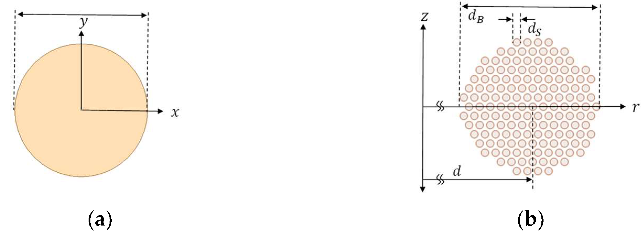
Figure 5a presents a single copper conductor modeled in a two-dimensional Cartesian coordinate system, representing an idealized condition where only strand-level skin effect is present. This simplified configuration facilitates theoretical analysis and allows direct comparison with the closed-form solution provided in Equation (6). Figure 5b illustrates a bundled arrangement of multiple conductors, Litz wire comprising a circular bundle of 150 conductors (44 AWG), analyzed in a 2-dimensional cylindrical coordinate system. This structure captures complex high-frequency phenomena, reflecting a more realistic and comprehensive electromagnetic behavior. Figure 6 presents the FEM simulation results of the AC resistance, R a c   F E M , along with the corresponding relative errors plotted for analysis in Figure 7.
Figure 7a shows the variation in the relative error between the simulated and analytical results with respect to the number of discretized segments. At low frequencies, the primary source of error originates from differences in cross-sectional area between the approximated polygon and the ideal circle. At higher frequencies above f δ , the perimeter mismatch becomes the dominant factor affecting accuracy. In contrast to the single-conductor case, which shows a relatively simple transition between saturation regions solely due to the skin effect, Figure 7b shows that the Litz wire comprising a circular bundle of 150 conductors has a more complex frequency-dependent pattern.
Mean absolute percentage error (MAPE) with segment variations in Table 1 represents the relative error between predicted and calculated values, exhibiting a clear decreasing trend as the segment number increases.
The MAPE in this paper is mathematically defined as follows:
1 n i = 1 n y i y ^ i y i × 100 ,
where y i , y ^ i , and n are the result, the reference value, and the number of data, respectively.
Finer segmentation improves the accuracy of the FEM model, minimizing the overall error rate for the both cases. However, beyond a certain number of segments, the rate of improvement diminishes.

3.2. Segment-Based Error Compensation Through Mathematical Fitting Models

The error pattern of R a c with frequency exhibits a characteristic sigmoidal behavior, transitioning from one asymptotic value to another. The hyperbolic tangent function effectively captures the observed pattern, making it a suitable choice for modeling. While a single hyperbolic tangent function accurately represents the skin effect in circular conductors, modeling the resistance variation in Litz wire bundles requires a double hyperbolic tangent model, which provides improved accuracy over the frequency range of interest.
The model is defined as follows:
C s = a 1 t a n h b 1 l o g f n + c 1 + a 2 t a n h b 2 l o g f n + c 2 + d .
The fitting parameters are obtained through curve fitting. The fitting process was conducted for each segment independently, leveraging curve-fitting algorithms to minimize the residual sum of squares between the calculated results and the FEM results. The coefficients corresponding to each segment are summarized in Table 2 and Table 3. In an isolated circular conductor, the frequency-dependent AC resistance follows a relatively simple response, and in the given equation, d represents the offset, while the ratio of c to b is an indication of the corner frequency.
The inverse of Function (9) was utilized to derive a frequency-dependent scaling factor to the corrected value, R a c   m o d . Figure 8 demonstrates the results applying the correction based on the proposed fitting model and its corresponding parameters. The results in Table 4 demonstrate that the fitting model maintains a MAPE well below 1%, regardless of the tested segment count. Figure 9 presents the error rate as a function of the normalized frequency. For an infinitely long isolated conductor, the error remains below 1% across the entire tested frequency range, demonstrating the suitability of the proposed approach. For the 150-strand (44 AWG) Litz wire, a 4-segment count shows unstable errors of approximately 3–4% above the skin-depth frequency in Figure 9b. When the number of segments is increased to six or more, the error remains stably below 1%. The current results show that, in the double-tanh model, the ratio of c   to b in the second term strongly affects the first corner frequency. We can observe that, relative to a circular conductor with no external field effect, the corner frequency in the 150-strand (44 AWG) Litz wire is reduced to less than one-tenth. The frequency-induced error becomes practically negligible and may be excluded as a variable in further analysis when this fitting model is applied regardless of whether the segment count is more than six.

3.3. Meshing Optimization for Low Element Count

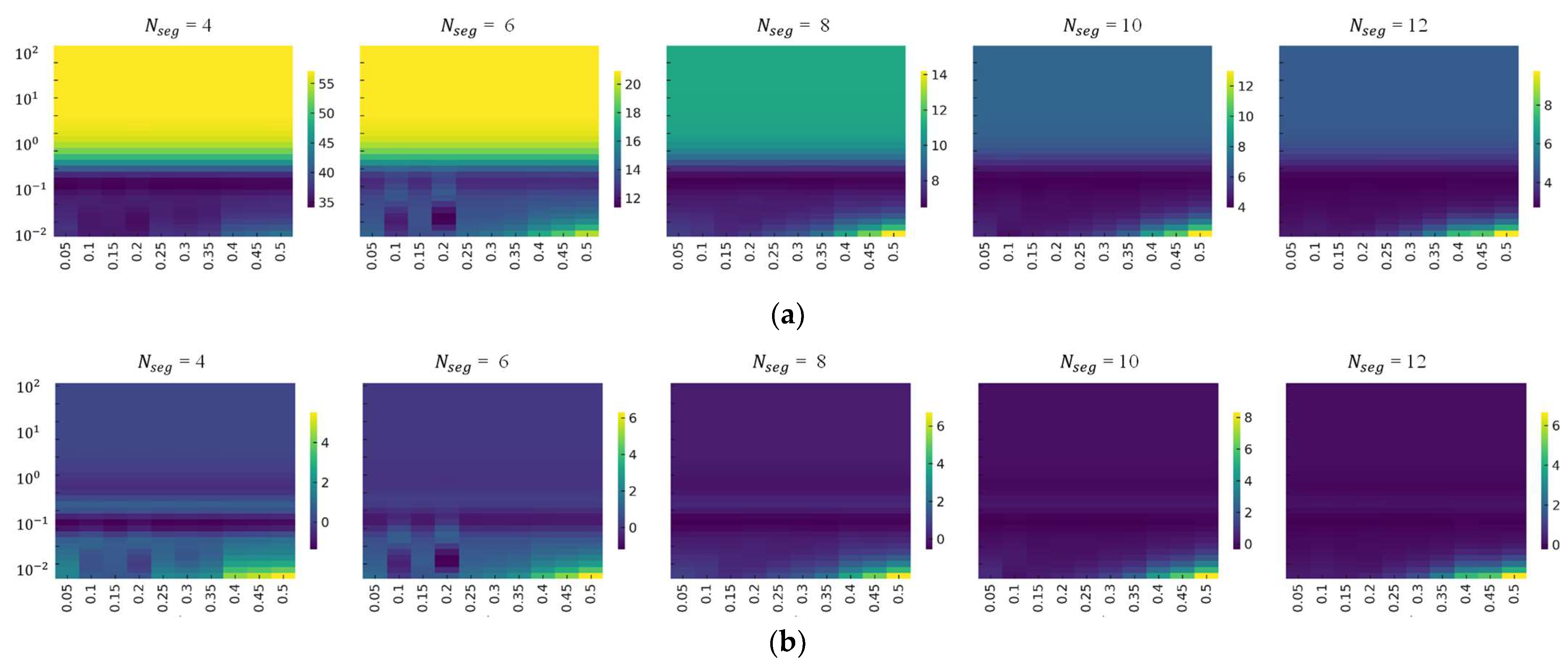
In numerical analysis, there is an inherent trade-off between computational cost and accuracy. In multi-strand configurations, such as Litz wire, an optimized meshing strategy is essential to enable efficient and accurate computation. One of the primary strategies for efficient resource utilization is boundary layer meshing, where finer mesh elements are concentrated near the conductor’s surface. Simulation data were generated by systematically varying three independent parameters, namely the number of polygonal segments N s e g , the number of mesh layers N s k i n , and the normalized skin mesh thickness ratio k s k i n = d s / D . For the initial analysis, the influence of the parameters on the MAPE (%) was evaluated in Figure 10. Using only a single mesh layer leads to unacceptably high errors, even after applying the proposed correction model, causing the use of a single-layer mesh impractical. When three or more mesh layers were used, the overall error remained consistently low, regardless of variations in other parameters; however, this inevitably increased the total element count. The use of two mesh layers with k s k i n   of 0.1 and 0.2 offers a favorable trade-off between accuracy and computational efficiency shown in Figure 10. This is primarily because of the alignment of the mesh-layer thickness, with the skin depths corresponding to frequencies that are 10 and 100 times higher than the operating frequency. By applying the proposed fitting model with an optimized meshing strategy, the error remains below 0.25% MAPE, even with a low segmentation count. Aligning the mesh-layer thickness with the skin depths corresponding to the frequencies of interest ensures high accuracy across the targeted frequency range.
Figure 11 illustrates the relative error, both before and after applying the fitting model, as a function of N s e g , k s k i n , and the normalized frequency, under the condition of using two mesh layers. Even with a segment count as low as four or six, configurations with k s k i n around 0.2 exhibit consistently low error levels, as shown in Figure 11b, demonstrating that the proposed correction method effectively compensates for discretization errors. Furthermore, it suggests that a meshing strategy aligned with the skin depths, particularly using two layers with a k s k i n around 0.2, can achieve both high accuracy and computational efficiency. Figure 12 illustrates the number of elements with N s e g and k s k i n . Notably, the case with six segments and twelve segments shows a lower element count than even the four-segment case where the k s k i n is 0.2. This indicates that six-segment partitioning or its multiples can offer higher computational efficiency. A six-segment division partitions the circle into 60° sectors, with each approximating an equilateral triangle in Figure 4. The generation of uniform triangular elements enables an efficient mesh with high accuracy. This observation highlights the importance of geometric symmetry in meshing strategies, as it facilitates uniform element distribution and minimizes numerical deviations across the simulation domain in FEM analyses. These results provide practical guidelines for selecting segmentation and meshing parameters that lead to an optimal balance between computational efficiency and solution accuracy. The six-segment case with mesh k s k i n = 0.2 and two mesh layers yields the lowest element count and the best performance under identical convergence conditions.

4. Experimental Validation of the Proposed 2D FEM-Based Modeling Approach

The 150-strand (44 AWG MW-80) Litz wire is used in the 12-turn and 21-turn winding as summarized in Table 5. The corresponding finite element models and the actual physical samples are illustrated in Figure 13. A two-dimensional finite element model of the 12-turn winding was constructed for the 150-strand Litz wire, comprising a total of 1800 segmented conductors, as illustrated in Figure 13b. Performing full 3D FEM simulations of structures with this level of complexity on personal computers is often infeasible due to memory limitations or excessively long computation times, which limits the feasibility of large-scale data generation. The 2D modeling of the Litz winding was implemented in a cylindrical coordinate system. Figure 14 illustrates the meshing layout and the resulting current density distribution at f n = 10 . A two-layer boundary mesh structure was employed, with the k s k i n set to 0.2. In the axisymmetric eddy current analysis performed on the rz-plane, the plane at z = 0 was assigned an even symmetry boundary condition, ensuring that the normal component of the magnetic flux density remains continuous across the boundary and that the magnetic field distribution is symmetric with respect to the z = 0 plane. This symmetry condition effectively reduced the element count by half. Details of the computational environment employed in this study are provided in Table 6. Figure 14 illustrates the meshing layout and resulting current density distribution in winding A at f n = 10 . Strand-level proximity effects from both internal and external fields are clearly observed in Figure 14.
To evaluate the computational efficiency and resource requirements of the proposed method, performance metrics and mesh statistics obtained from FEM simulations were analyzed with different segment counts, as summarized in Table 7 and Table 8. FEM computation consists of three stages, namely validation, meshing, and analysis. Validation initializes data structures and verifies the model, while analysis, which solves the equations, accounts for most of the total computation time. As the number of segments increased from 4 to 12, the total simulation time rose from 3272 s to 7886 s. In parallel, memory usage also exhibited a substantial increase, from 12.0 GB at 4 segments to 35.4 GB at 12 segments. This increase correlates with the number of elements in the strands, which rose from 18,889 to 57,158. These results demonstrate that both computational load and simulation time vary significantly with the segment count.
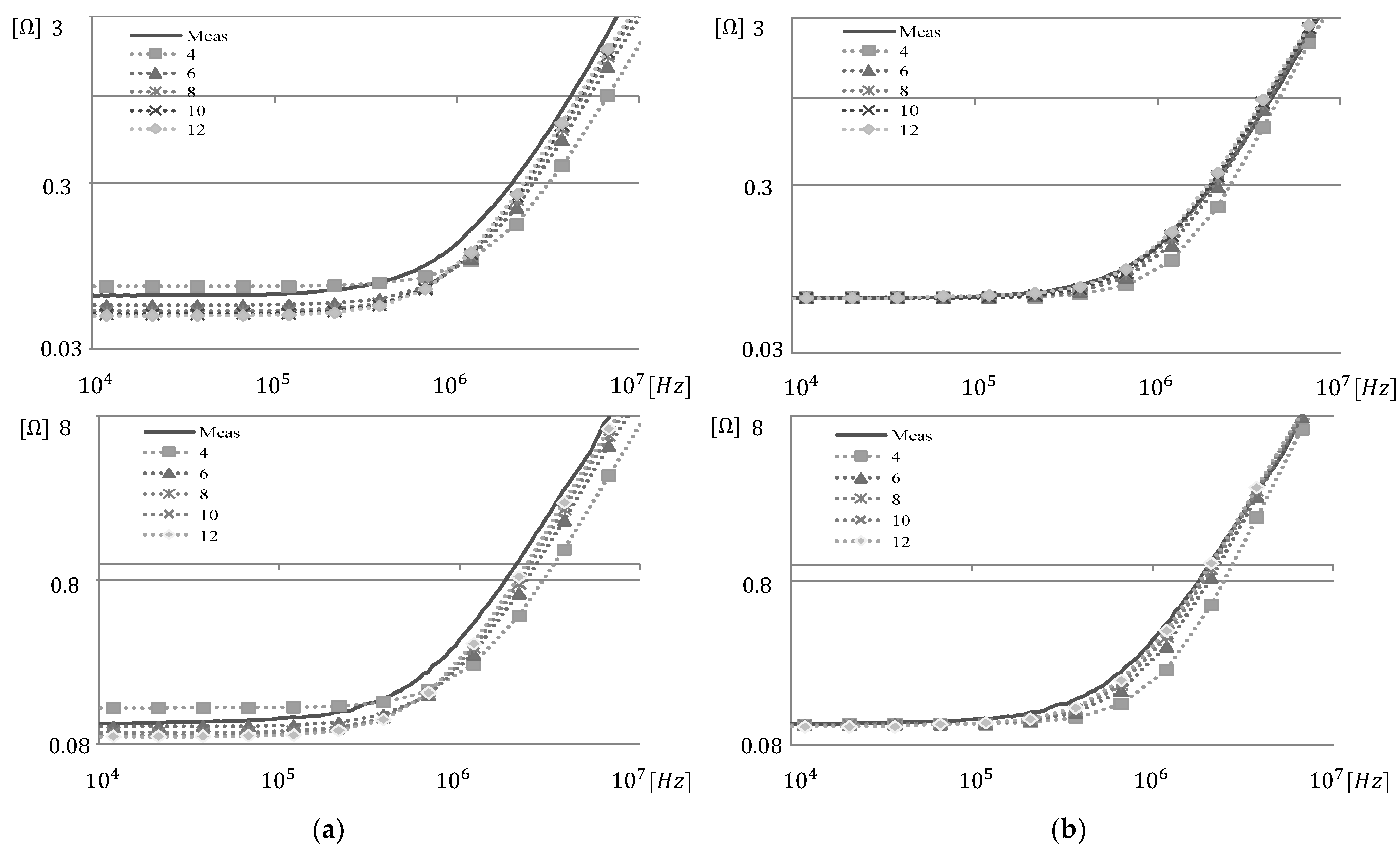
The impedance measurements were performed at room temperature using an Agilent 4294A precision impedance analyzer. The measured AC resistance R a c   M e s   of the windings was compared with results from the proposed model with the segment counts in Figure 15. In practical winding structures with a large number of turns and layers, the error introduced by geometric simplification tends to increase. In particular, the four-segment case shows a visible deviation near the corner frequency. Nevertheless, when the number of segments is six or more, the application of the proposed fitting model enables predictions with an accuracy that remains within acceptable limits. This reflects an inherent trade-off, where the choice of segmentation can be made according to the required design specifications. While finer segmentation improves accuracy by enabling denser meshing, the incremental accuracy gain may be marginal in practical scenarios, especially when considering structural imperfections and measurement uncertainties.

5. Conclusions

This study proposes a practical and readily applicable framework for accurately analyzing electromagnetic phenomena in Litz windings and predicting their AC resistance using commercially available 2D FEM tools on standard personal computing systems. By integrating optimized meshing strategies with a hyperbolic tangent fitting function, the framework effectively mitigates geometric discretization errors in circular conductors while reducing computational cost across the normalized frequency range from 10 2 and 10 2 , which is highly relevant to practical engineering applications. Aligning the mesh-layer thickness with skin depths corresponding to the frequencies of interest achieves high accuracy while minimizing the number of elements. Furthermore, by applying the proposed fitting model, the reduced number of segments can decrease the computational load and time to a similar extent, while maintaining comparable accuracy. The combination of 6 segments, a 2-layer boundary mesh, and a mesh depth ratio of 0.2 yielded optimal results under the tested conditions due to the structural symmetry of hexagonal partitioning, showing excellent agreement with measurement results. As the number of turns and layers in the winding increases, the effectiveness of structural simplification and correction via fitting models tends to decrease. However, when six or more segments are used under optimal meshing conditions, the error is sufficiently reduced to an acceptable range in practice. In addition, the segment counts and meshing conditions can be appropriately adjusted based on the desired trade-off between accuracy and computational efficiency. The proposed 2D FEM-based framework for AC resistance modeling of Litz wire windings is highly practical for engineering environments utilizing standard desktop computing systems and can be readily applied to the design and optimization of modern magnetic components, such as high-frequency transformers, EMI filters, and wireless power transfer (WPT) systems.

Funding

This research was supported by the BisaResearch Grant of Keimyung University in 2021 (Project No: 20220649).

Institutional Review Board Statement

Not applicable.

Informed Consent Statement

Not applicable.

Data Availability Statement

The original contributions presented in the study are included in the article, further inquiries can be directed to the corresponding author.

Acknowledgments

The author would like to thank the technical support from Ansys Korea.

Conflicts of Interest

The author declares no conflicts of interest.

References

  1. Jaritz, M.; Biela, J. Analytical Model for the Thermal Resistance of Windings Consisting of Solid or Litz Wire. In Proceedings of the 2013 15th European Conference on Power Electronics and Applications (EPE), Lille, France, 2–6 September 2013; pp. 1–10. [Google Scholar]
  2. Baek, S.; Bhattacharya, S. Analytical Modeling and Implementation of a Coaxially Wound Transformer with Integrated Filter Inductance for Isolated Soft-Switching DC–DC Converters. IEEE Trans. Ind. Electron. 2018, 65, 2245–2255. [Google Scholar] [CrossRef]
  3. Ahmed, D.; Wang, L. Optimal Area-Product Model (OAPM) Based Non-Iterative Analytical Design Methodology for Litz-Wired High-Frequency Gapped-Transformer (LHFGT) in LLC Converters. IEEE Access 2020, 8, 18134–18148. [Google Scholar] [CrossRef]
  4. Deng, Q.; Liu, J.; Czarkowski, D.; Kazimierczuk, M.K.; Bojarski, M.; Zhou, H. Frequency-Dependent Resistance of Litz-Wire Square Solenoid Coils and Quality Factor Optimization for Wireless Power Transfer. IEEE Trans. Ind. Electron. 2016, 63, 2825–2837. [Google Scholar] [CrossRef]
  5. Prosen, N.; Domajnko, J.; Milanovič, M. Wireless Power Transfer Using Double-DD Coils. Electronics 2021, 10, 2528. [Google Scholar] [CrossRef]
  6. Dowell, P.L. Effects of Eddy Currents in Transformer Windings. Proc. IEE 1966, 113, 1387–1394. [Google Scholar] [CrossRef]
  7. Ferreira, J.A. Improved Analytical Modeling of Conductive Losses in Magnetic Components. IEEE Trans. Power Electron. 1994, 9, 127–131. [Google Scholar] [CrossRef]
  8. Ferreira, J.A. Appropriate Modelling of Conductive Losses in the Design of Magnetic Components. In Proceedings of the 21st Annual IEEE Conference on Power Electronics Specialists (PESC), San Antonio, TX, USA, 11–14 June 1990. [Google Scholar]
  9. Albach, M. Two-Dimensional Calculation of Winding Losses in Transformers. In Proceedings of the 2000 IEEE 31st Annual Power Electronics Specialists Conference (PESC), Galway, Ireland, 23–23 June 2000. [Google Scholar]
  10. Vandelac, J.P.; Ziogas, P.D. A Novel Approach for Minimizing High-Frequency Transformer Copper Losses. IEEE Trans. Power Electron. 1988, 3, 266–277. [Google Scholar] [CrossRef]
  11. Hurley, W.G.; Gath, E.; Breslin, J.G. Optimizing the AC Resistance of Multilayer Transformer Windings with Arbitrary Current Waveforms. IEEE Trans. Power Electron. 2000, 15, 369–376. [Google Scholar] [CrossRef]
  12. Wallmeier, P. Improved Analytical Modeling of Conductive Losses in Gapped High-Frequency Inductors. IEEE Trans. Ind. Appl. 2001, 37, 1045–1054. [Google Scholar] [CrossRef]
  13. Lotfi, A.W.; Lee, F.C. A High Frequency Model for Litz Wire for Switch-Mode Magnetics. In Conference Record of the 1993 IEEE Industry Applications Conference Twenty-Eighth IAS Annual Meeting, Toronto, ON, Canada, 2–8 October 1993; Volume 2, pp. 1169–1175. [Google Scholar]
  14. Arruti, E.; Stevanovic, M.; Krizmanic, K.; Hjuler, K. Evolution of Classical 1-D Based Models and Improved Approach for the Characterization of Litz Wire Losses. IEEE Trans. Power Electron. 2024; early access. [Google Scholar] [CrossRef]
  15. Sullivan, C.R. Optimal Choice for Number of Strands in a Litz-Wire Transformer Winding. IEEE Trans. Power Electron. 1999, 14, 283–291. [Google Scholar] [CrossRef]
  16. Sullivan, C.R.; Zhang, R.Y. Simplified Design Method for Litz Wire. In Proceedings of the IEEE Power Electronics Specialists Conference (PESC), Fort Worth, TX, USA, 16–20 March 2014; pp. 2667–2674. [Google Scholar]
  17. Sullivan, C.R.; Zhang, R.Y. Analytical Model for Effects of Twisting on Litz-Wire Losses. In Proceedings of the IEEE Workshop on Control and Modeling for Power Electronics (COMPEL), Santander, Spain, 22–25 June 2014; pp. 1–10. [Google Scholar]
  18. Tang, X.; Sullivan, C.R. Stranded Wire with Uninsulated Strands as a Low-Cost Alternative to Litz Wire. In Proceedings of the 34th Annual Conference on Power Electronics Specialists (PESC ‘03), Acapulco, Mexico, 15–19 June 2003. [Google Scholar]
  19. Ahmadi, S.; Khan, S.H.; Grattan, K.T.V. Impact of Twisting on Skin and Proximity Losses in Segmented Underground Cables: A 3D Finite-Element Study. Appl. Sci. 2025, 15, 2814. [Google Scholar] [CrossRef]
  20. Rossmanith, H.; Dobrotenko, M.; Albach, M.; Exner, D. Measurement and Characterization of High Frequency Losses in Nonideal Litz Wires. IEEE Trans. Power Electron. 2018, 33, 7828–7840. [Google Scholar] [CrossRef]
  21. Plumed, E.; Acero, J.; Lope, I.; Carretero, C. 3D Finite Element Simulation of Litz Wires with Multilevel Bundle Structure. In Proceedings of the 2018 IEEE 44th IECON, Washington, DC, USA, 21–23 October 2018; pp. 3479–3484. [Google Scholar]
  22. Otomo, Y.; Igarashi, H.; Sano, H.; Yamada, T. Analysis of Litz Wire Losses Using Homogenization-Based FEM. IEEE Trans. Magn. 2021, 57, 7402409. [Google Scholar] [CrossRef]
  23. Zhang, R.Y.; White, J.K.; Sullivan, C.R. Realistic Litz Wire Characterization Using Fast Numerical Simulations. IEEE Trans. Power Electron. 2020, 35, 12642–12655. [Google Scholar]
  24. Lyu, J.; Chen, H.; Zhang, Y.; Du, Y.; Cheng, Q.S. Fast Simulation of Litz Wire Using Multilevel PEEC Method. IEEE Trans. Power Electron. 2020, 35, 12612–12623. [Google Scholar] [CrossRef]
  25. Ehrlich, S.; Rossmanith, H.; Sauer, M.; Joffe, C.; März, M. Fast Numerical Power Loss Calculation for High-Frequency Litz Wires. IEEE Trans. Power Electron. 2021, 36, 2018–2031. [Google Scholar] [CrossRef]
  26. Zhang, R.Y.; White, J.K.; Sullivan, C.R.; Kassakian, J.G. Fast Simulation of Complicated 3D Structures above Lossy Magnetic Media. In Proceedings of the 2017 IEEE 18th Workshop on Control and Modeling for Power Electronics (COMPEL), Stanford, CA, USA, 9–12 July 2017; pp. 1–7. [Google Scholar]
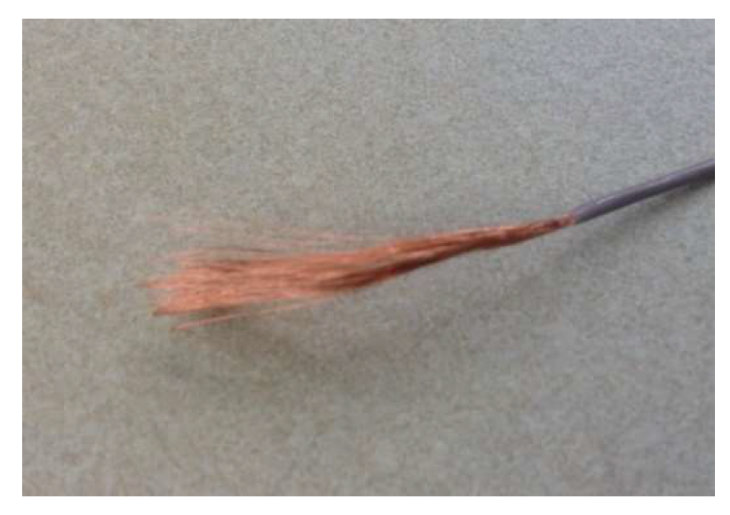
Figure 1. A typical Litz wire composed of 150 twisted and woven insulated strands.
Applsci 15 09185 g001
Figure 2. High-frequency effects in multi-strand conductors. (a) Strand-level skin effect; (b) bundle-level skin effect; (c) strand-level proximity effect; (d) bundle-level proximity effect.
Applsci 15 09185 g002
Figure 3. (a) A current-carrying infinitely long conductor; (b) F s k i n vs. r δ .
Applsci 15 09185 g003
Figure 4. Polygonal approximation of circular geometry and current density at f n = 10 .
Applsci 15 09185 g004
Figure 5. (a) 2D representation of a single conductor; (b) 2D representation of a bundle of 150 strands (44 AWG); d B = 0.9   m m ,   d s = 0.05   m m ,   d = 10   m m .
Applsci 15 09185 g005
Figure 6. (a) R a c   F E M of a single conductor vs. f n ; (b) R a c   F E M of a 150-strand (44 AWG) Litz wire vs. f n .
Applsci 15 09185 g006
Figure 7. (a) Relative error [%] of a single conductor vs. f n ; (b) relative error [%] of a 150-strand (44 AWG) Litz wire vs. f n .
Applsci 15 09185 g007
Figure 8. (a) R a c of a single conductor vs. f n after correction; (b) R a c of a 150-strand (44 AWG) Litz wire vs. f n after correction.
Applsci 15 09185 g008
Figure 9. (a) Relative error (%) of a single conductor vs. f n after correction; (b) relative error (%) of a 150-strand (44 AWG) Litz wire vs. f n after correction.
Applsci 15 09185 g009
Figure 10. MAPE (%) vs. N s e g and k s k i n . (a) Layer = 1 before correction (top) and after correction (bottom); (b) layer = 2 before correction (top) and after correction (bottom); (c) layer = 3 before correction (top) and after correction (bottom).
Applsci 15 09185 g010
Figure 11. Percentage error [%] vs. N s e g   for segment count ( N s k i n = 2 ). (a) Before applying the fitting model; (b) after applying the fitting model.
Applsci 15 09185 g011
Figure 12. The number of elements vs. N s e g , k s k i n (a) N s k i n = 1 ; (b) N s k i n = 2 ; (c) N s k i n = 3 .
Applsci 15 09185 g012
Figure 13. (a) Litz winding; (b) 2D FEM model for winding A (12 turns); (c) 2D FEM model for winding B (21 turns).
Applsci 15 09185 g013
Figure 14. Current density and mesh distribution of the winding at f n = 10 (a) N s e g = 4 ; (b) N s e g = 6 ; (c) N s e g = 8 ; (d) N s e g = 10 ; (e) N s e g = 12 .
Applsci 15 09185 g014
Figure 15. (a) R a c   F E M and R M e a s vs. frequency before applying the fitting model for winding A (top) and winding B (bottom); (b) R a c   F E M and R M e a s vs. frequency after applying the fitting model for winding A (top) and winding B (bottom).
Applsci 15 09185 g015
Table 1. MAPE (%) of R a c .
Segment4681012
A single conductor45.17415.1357.04953.5591.751
a 150-44 AWG Litz wire24.3079.2044.5712.3311.166
Table 2. Double hyperbolic tangent model parameters for a single circular conductor.
Segment a 1 b 1 c 1 a 2 b 2 c 2 d
44.4622.308−1.8044.561−2.2681.7851.431
61.0061.222−0.7011.040−1.2130.7131.144
85.0579.686−5.8945.071−6.5914.1121.068
102.7919.190−5.5922.798−6.6444.1261.034
122.1579.343−5.6592.160−7.0414.3341.016
Table 3. Double hyperbolic tangent model parameters for a 150-strand (44 AWG) Litz wire.
Segment a 1 b 1 c 1 a 2 b 2 c 2 d
40.2241.847−2.0600.487−1.074−1.2561.265
60.1311.260−1.1160.213−1.020−1.1441.096
85.6960.7570.3035.729−0.762−0.3291.050
100.0620.848−0.3630.079−0.910−0.8141.024
122.2420.7510.3632.250−0.755−0.3811.012
Table 4. MAPE (%) of R a c after correction using the double hyperbolic tangent model.
Segment4681012
A single conductor0.1280.2240.0730.0560.030
A 150-44 AWG Litz wire0.7560.1740.2580.1390.093
Table 5. Specifications of Litz wire winding.
The Number of Layers/TurnsBundle/Strand
Winding A2/12150-strand (44 AWG) enameled wire, copper,
D B = 0.9   m m ,   D s = 0.05   m m ,   d = 10   m m
Winding B3/13
Table 6. Specifications of the computing environment used for FEM.
Operating
System
Processor/RAMFrequency RangePercent
Error
Windows 11
x64-based PC
Intel® Core™ i7-14700KF 3.40GHz
/64GB
4.71 kHz~47.1 MHz
logarithmic scale, 4 points/decade
0.6%
Table 7. Computational time [s] in winding A ( N s k i n = 2, k s k i n = 0.2).
N s e g ValidationMeshing AnalysisTotal Elapsed Time
414593817753272
620444524274516
825015329455499
1030146135496624
1236077342067886
Table 8. Memory consumption and number of elements in winding A ( N s k i n = 2, k s k i n = 0.2).
N s e g Memory Usage [GB]Total Number of Elements in StrandsThe Average Number of Elements in a Strand
412.018,88910.49
617.829,87116.60
823.737,75920.98
1029.545,75625.42
1235.457,15831.75
Disclaimer/Publisher’s Note: The statements, opinions and data contained in all publications are solely those of the individual author(s) and contributor(s) and not of MDPI and/or the editor(s). MDPI and/or the editor(s) disclaim responsibility for any injury to people or property resulting from any ideas, methods, instructions or products referred to in the content.