DFF: Sequential Dual-Branch Feature Fusion for Maritime Radar Object Detection and Tracking via Video Processing

Abstract

Robust maritime radar object detection and tracking in maritime clutter environments is critical for maritime safety and security. Conventional Constant False Alarm Rate (CFAR) detectors have limited performance in processing complex-valued radar echoes, especially in complex scenarios where phase information is critical and in the real-time processing of successive echo pulses, while existing deep learning methods usually lack native support for complex-valued data and have inherent shortcomings in real-time compared to conventional methods. To overcome these limitations, we propose a dual-branch sequence feature fusion (DFF) detector designed specifically for complex-valued continuous sea-clutter signals, drawing on commonly used methods in video pattern recognition. The DFF employs dual parallel complex-valued U-Net branches to extract multilevel spatiotemporal features from distance profiles and Doppler features from distance–Doppler spectrograms, preserving the critical phase–amplitude relationship. Subsequently, the sequential feature-extraction module (SFEM) captures the temporal dependence in both feature streams. Next, the Adaptive Weight Learning (AWL) module dynamically fuses these multimodal features by learning modality-specific weights. Finally, the detection module generates the object localisation output. Extensive evaluations on the IPIX and SDRDSP datasets show that DFF performs well. On SDRDSP, DFF achieves 98.76% accuracy and 68.75% in F1 score, which significantly outperforms traditional CFAR methods and state-of-the-art deep learning models in terms of detection accuracy and false alarm rate (FAR). These results validate the effectiveness of DFF for reliable maritime object detection in complex clutter environments through multimodal feature fusion and sequence-dependent modelling.

1. Introduction

Radar is celebrated for its ability to operate continuously across all environmental conditions, with a proven aptitude for long-range object detection and tracking. Unlike optical object detection and tracking, radar functionality remains impervious to illumination-dependent factors. Maritime radar object detection leverages temporal sequences of pulse echoes, analogous to video-frame processing, where each pulse represents a temporal snapshot of the marine environment. However, radar echoes exhibit a complex composition, encompassing not only object signals but also interference, sea clutter, and nearshore reflections, which collectively render maritime object detection highly complex. Sea clutter is influenced by a multivariate landscape of factors, including intrinsic wave height, wind speed, sea state, and radar-specific parameters (e.g., grazing angle, azimuth, pulse repetition frequency, antenna polarisation, and operational settings). As such, accurately modelling sea clutter with a single statistical framework—whether based on Rayleigh, log-normal, or K-distributions—remains a formidable challenge. This spatiotemporal complexity resembles dynamic video scenes with varying illumination and occlusion patterns. Early echo-detection techniques relied heavily on mathematical statistics, rooted in parametric modelling and hypothesis testing; paradigmatic examples include CA-CFAR [1] and GO-CFAR [2], both grounded in the CFAR paradigm. While these conventional approaches [1,2] offer computational simplicity and efficiency, their performance degrades significantly in complex maritime environments with non-stationary clutter, primarily due to their inability to model temporal dependencies across pulses, a capability inherent to video processing frameworks. Deep learning methods like DBCNN [3] and Multi-Branch-CNN [4] improve representation but still struggle with phase information preservation and real-time processing of sequential radar pulses.

The advent of machine learning introduced a new paradigm for radar echo analysis, where researchers began designing handcrafted features [5,6,7] to enhance object classification. Similar to early video action recognition methods, a typical workflow involves time-frequency domain analysis to derive discriminative features [8,9,10], which are subsequently used to segregate pure clutter from target-laden echoes. While these methods exhibit flexibility across varying SNR and SCR regimes, their performance is inherently limited by the same feature engineering constraints that plagued early video analysis techniques. Additionally, in low-SNR environments, multi-target scenarios, or dynamic interference conditions, these approaches suffer from high false alarm rates and computational inefficiency, much like video processing in low-light or occluded conditions. They also demonstrate pronounced sensitivity to training data distributions, with performance degrading sharply when tested under divergent environmental conditions.

Drawing inspiration from breakthroughs in video temporal modelling, recent deep learning approaches have propelled radar analysis to new heights. Deep learning’s representation capabilities, proven successful across video modalities [11,12,13,14,15,16], motivate our maritime radar detection model. Inspired by video temporal modelling breakthroughs like STVSR [17], we treat radar pulse sequences as spatiotemporal signals analogous to video streams. We specifically address two critical gaps: (1) the intrinsic complexity of radar echoes as spatiotemporal signals comparable to video streams, and (2) the limitations of conventional architectures in processing such data. Our solution adapts video processing principles by modifying standard modules to handle complex-valued inputs, preserving spatiotemporal phase–amplitude relationships essential for discrimination. Furthermore, we address heterogeneous clutter challenges [18] through multimodal fusion techniques inspired by video–audio integration methods, particularly crucial for differentiating small objects, such as buoys, from large ships in high-clutter regimes. The inherent limitation of single-modality approaches [19] reflects the early video-recognition systems’ inability to integrate motion and appearance features.

To address these challenges, we reformulate radar detection as a spatiotemporal processing task analogous to video analysis. Radar echoes’ slow-time pulse sequences exhibit frame-like temporal dependencies, enabling processing through video-inspired architectures. Specifically, we jointly ingest sequences of pulse range profiles (spatial amplitude evolution) and range–Doppler maps (Doppler kinematics) as dual-modality spatiotemporal inputs. The model employs:

• Video-Inspired Spatiotemporal Processing: We introduce a joint processing framework for pulse sequences and Doppler maps, enabling coherent object tracking through range cells using temporal coherence principles from video object tracking.
• Complex-Valued Video Adaptations: We modify neural modules to process radar sequences as spatiotemporal volumes natively, preserving phase information as critically as optical flow in video analysis.
• Adaptive Multi-modal Fusion: We implement feature weighting mechanisms derived from video–audio attention models to enhance clutter discrimination in dynamic marine environments.

While existing video-inspired radar methods [11,13,18] treat radar sequences as frame-like inputs, they fundamentally differ from optical video in two key aspects: (1) Radar pulses contain complex-valued phase relationships critical for Doppler discrimination, and (2) Temporal dependencies manifest as pulse-to-pulse phase coherence rather than pixel motion. DFF advances beyond these methods by:

• Native Complex Processing: Preserving phase–amplitude relationships through end-to-end complex-valued operations (vs. real-valued approximations in [13]).
• Radar-Specific Fusion: Adaptively weighting range–pulse and range–Doppler features via AWL (contrasting with rigid concatenation in [18]).
• Pulse-Centric Modelling: Optimising SFEM for slow-time pulse sequences rather than video frame rates.

2. Related Work

2.1. Statistical Methods for Maritime Object Detection

Traditional radar object detection relies heavily on statistical frameworks, withCFAR (CFAR) algorithms forming the cornerstone of this approach. CA-CFAR [1] and OS-CFAR [20] establish adaptive detection thresholds through localised clutter modelling, yet fundamentally operate under a pulse-isolated processing paradigm that neglects inter-pulse dependencies. This limitation manifests as persistent false alarms during sea spikes [21] and meteorological interference [22], while their exclusive amplitude-domain processing discards critical phase information. Although variants like Amrit et al.’s nonlinear compression CFAR [23] improve robustness against non-uniform clutter, they remain constrained by parametric assumptions that fail to capture the non-stationary time-frequency characteristics of complex marine environments [24]. These intrinsic limitations necessitate novel approaches capable of modelling temporal dependencies while fully utilising complex signal information for maritime object detection.

2.2. Machine Learning Advancements with Feature Engineering

Building upon statistical foundations, machine learning methods introduced data-driven feature engineering for enhanced clutter discrimination in object detection. Gao et al.’s RFrFT canceller [8] and Chen et al.’s STFrFT [10] pioneered time-frequency transformations that extract micro-motion characteristics of objects, while Zhang et al.’s sequence feature representation [6] exploited temporal correlations between objects and clutter. Lu et al.’s HOG-SVM framework [25] further demonstrated the potential of combining spatial features with classifiers for object recognition. However, these approaches face three fundamental constraints: (1) handcrafted features cannot comprehensively characterise complex clutter dynamics; (2) the decoupled feature extraction and classification pipeline limits adaptability to varying marine conditions; and (3) significant performance degradation occurs under low-SNR conditions [26]. Yan et al.’s MSR detector [27] exemplifies these challenges, while eliminating prior model assumptions, its efficacy diminishes in practical low-SNR scenarios for object identification. Besides, Other early approaches relied on feature engineering, e.g., PseKRAAC [22] and wavelet transforms [28], but handcrafted features lack adaptability to dynamic sea conditions [29].

2.3. Deep Learning Paradigms and Current Limitations

The advent of deep learning revolutionised maritime radar object detection through end-to-end feature learning, yet significant challenges persist in complex clutter environments:

Real-valued architectures like Pei et al.’s CycleGAN [11] and Wang et al.’s attention models [13] achieve notable performance but fundamentally discard critical phase information by processing complex data as separate real-imaginary channels. This limitation parallels Wang et al.’s observation [14] that semi-supervised frameworks struggle when teacher models lack phase-sensitive representations of objects.

Complex-valued networks pioneered by Lei et al. [30] and advanced by Wang et al. [18] directly process amplitude-phase pairs, preserving coherence relationships essential for micro-motion feature extraction of marine objects. These demonstrate 8–50% performance gains over real-valued counterparts in sidelobe interference scenarios for object recognition. Recent breakthroughs in complex-valued deep learning [31,32] have demonstrated significant improvements in phase-sensitive tasks, validating our architectural choices.

Multi-modal fusion approaches like Wang et al.’s conditional GAN [19] integrate CFAR controllers with deep features, maintaining 96% object recognition rates at SCR = $-10$ dB. However, current methods exhibit three persistent limitations: inadequate modelling of pulse-sequence dependencies for objects, insufficient joint spatiotemporal representation learning [33], and suboptimal adaptive fusion of heterogeneous features affecting object discrimination [34]. Overall, emerging multimodal fusion techniques [35,36] provide theoretical foundations for our adaptive weighting approach.

2.4. Unresolved Research Challenges

Current maritime radar object detection systems confront three fundamental challenges: (1) inadequate modeling of pulse-sequence dependencies, where existing methods fail to fully exploit temporal correlations across pulses for robust object tracking; (2) insufficient integration of joint spatiotemporal representations, as limited architectures effectively combine spatial features with the temporal evolution of objects; and (3) suboptimal adaptive multi-modal fusion, where crude feature concatenation neglects the modality-specific information value essential for precise object characterization. To address these challenges simultaneously, our DFF detector implements a comprehensive solution framework: the SFEM captures pulse-to-pulse temporal correlations through advanced sequence modelling, inspired by recurrent neural networks (RNNs) [37], which effectively models long-range dependencies, similar to the GRU-based quality fusion [38], enhancing feature integration across pulses. Dual-branch complex-valued U-Net enables hierarchical spatiotemporal learning that preserves phase–amplitude relationships, and the AWL fusion mechanism employs attention-based feature weighting to dynamically integrate heterogeneous modalities, collectively enabling robust object detection in complex sea clutter environments.

3. Methodology

3.1. Problem Analysis and Data Representation

Maritime radar emits N coherent linear frequency-modulated pulses for sea-surface object detection. The resulting range profile $\mathbf{R}\in {\mathbb{C}}^{N\times M}$ is constructed through fast-time sampling, where M denotes range units. Given that object velocity $V\ll c$, object echoes exhibit thermal stability in $\mathbf{R}$, while sea clutter displays significant fluctuations due to complex sea-surface dynamics.

As illustrated in Figure 1, using the “20221115080041_staring_HH” sub-dataset of the Sea-Detecting Radar Data-Sharing Program (SDRDSP) Dataset published by Guan et al. [39], Buoy 1 (range cells 501–513) and Buoy 2 (673–681) demonstrate distinct intensity profiles compared to surrounding clutter. Crucially, as shown in Figure 2, object-clutter discrimination is enhanced through Doppler characteristics: object echoes exhibit concentrated energy in narrow Doppler bands, while clutter shows dispersed spectral energy.

The distance image and range–Doppler spectrum represent the echo characteristics from different angles. It is the main purpose of this paper to build a suitable detector to extract and efficiently fuse the fast and slow time characteristics and range–Doppler characteristics from the distance image and range–Doppler spectrum to improve the detector’s performance.

3.2. Video-Inspired Architecture Design

The proposed dual-branch feature fusion (DFF) model harnesses the complementarity of two distinct feature types to jointly conduct object echo recognition, as depicted in Figure 3. Each branch uses a complex-valued U-Net to extract spatial features per pulse slice (treating Distance as the spatial axis). The SFEM then models temporal dependencies across pulses (Pulse Index dimension), similar to how temporal convolutional networks process sequential data.

At the core of the architecture, DFF incorporates an SFEM to capture temporal correlations along the sequence dimension from both raw inputs and high-dimensional features extracted by the branches. These correlations correspond to the slow-time (pulse) dimension of range profiles and the Doppler dimension of range–Doppler maps. The SFEM, situated within the contracting paths of both branches, transfers extracted sequential features to their counterpart modules in the expanding paths. Meanwhile, the SFEM in the expanding paths forwards processed features to the detection module, which localises objects within specific range cells.

Fast/slow time features and range–Doppler features complementarily characterise the discriminative properties of objects and clutter. Leveraging the collaborative interplay of these modules, the detector effectively extracts and fuses multi-modal features from range profiles and range–Doppler maps, thereby enhancing detection performance. Subsequent sections detail the components of the proposed detector.

3.3. Hierarchical Feature-Extraction Architecture

The DFF model, inspired by [40], employs dual U-Net-style branches [41] for complementary feature extraction: the upper branch processes range profiles to capture fast/slow time characteristics, while the lower branch analyses range–Doppler spectrograms for Doppler feature extraction. Each branch implements a symmetrical encoder-decoder architecture—the encoder comprises stacked complex-valued CBR (Convolution-BatchNorm-ReLU) blocks with max-pooling layers, progressively downsampling features to distil multi-scale spatiotemporal representations; conversely, the decoder utilises transposed convolutions and skip connections to restore resolution while fusing three critical inputs: (i) same-level encoder features, (ii) sequential features from SFEM, and (iii) upsampled outputs from preceding decoder layers. To enhance training efficiency and generalisation, auxiliary detection heads are appended to both decoders, generating preliminary outputs that preserve modality-specific characteristics through independent weight initialisation and optimisation.

The core building block, the complex-valued CBR module shown in Figure 4, implements a sequential processing pipeline optimised for radar data: $1\times 3$ convolutions along the range dimension encode fast-time dependencies, batch normalisation standardises complex-valued feature distributions, and complex ReLU activations introduce essential nonlinearity while preserving phase–amplitude relationships—collectively mitigating performance degradation in deep architectures. This modular design enables consistent feature extraction across both pulse-range profiles and range–Doppler maps while maintaining native complex-domain processing for all convolutional, pooling, and normalisation operations.

Complex Convolution: Given a complex-valued input tensor or feature map $\mathbf{Z}=\mathbf{X}+i\mathbf{Y}$ and a complex-valued convolution kernel $\mathbf{W}=\mathbf{A}+i\mathbf{B}$, the convolution operation is defined as follows:

$$\mathbf{W}\ast \mathbf{Z}=(\mathbf{A}\ast \mathbf{X}-\mathbf{B}\ast \mathbf{Y})+i(\mathbf{A}\ast \mathbf{Z}+\mathbf{B}\ast \mathbf{X})$$

This form preserves the complex algebraic structure while ensuring that the phase–amplitude relationship remains intact [42]. Specifically, complex-valued convolution uses a complex Gaussian distribution to initialise the convolution kernel, i.e., if the complex-valued Gaussian Distribution is $\mathbf{z}=\mathbf{x}+i\mathbf{y}$, and statisfies $x\sim ({\mu }_x,{\sigma }_x^2)$, $y\sim ({\mu }_y,{\sigma }_y^2)$, $\mu ={\mu }_x={\mu }_y$, $\sigma ={\sigma }_x^2={\sigma }_y^2$, then ${\mu }_z={\mu }_x+i{\mu }_y,{\sigma }_z^2=2{\sigma }_x^2=2{\sigma }_y^2$. Based on the Wirtinger derivative [43], the gradient of the loss function L to the complex-valued convolution kernel $\mathbf{W}$ is

$${\nabla }_{\mathbf{W}}\mathrm{L}={\displaystyle \frac{\partial \mathrm{L}}{\partial {\mathbf{W}}^{\ast }}}={\left({\displaystyle \frac{\partial \mathrm{L}}{\partial \mathbf{A}}}+i{\displaystyle \frac{\partial \mathrm{L}}{\partial \mathbf{B}}}\right)}^{\ast }$$

where ∗ denotes the complex conjugate.

Complex Batch Normalization: For complex feature $\mathbf{Z}$, normalization is achieved by jointly normalising the real and imaginary parts:

$$\widehat{\mathbf{Z}}=\gamma \odot {\displaystyle \frac{\mathbf{Z}-\mu }{\sigma }}+\beta$$

where $\mu =\mathrm{E}\left[\mathbf{Z}\right]$, $\sigma =\sqrt{\mathrm{E}\left[\right|\mathbf{Z}-\mu {|}^2]}$, $\gamma ,\beta \in {\mathbb{R}}^d$ is learnable parameters.

Complex ReLU (CReLU): For complex-valued features $\mathbf{Z}$, CReLU is defined as

$$\mathrm{CReLU}\left(\mathbf{Z}\right)=\mathrm{ReLU}\left(\mathbf{X}\right)+i·\mathrm{ReLU}\left(\mathbf{Y}\right)$$

This form is able to maintain phase continuity while introducing nonlinearity [44].

3.4. Sequential Feature Extraction and Fusion

3.4.1. Temporal Modeling Fundamentals

Radar pulse sequences exhibit two key temporal properties critical for maritime target detection:

• Phase Coherence: Target echoes maintain pulse-to-pulse phase consistency due to rigid-body kinematics, whereas sea clutter shows random phase jumps from surface dynamics.
• Doppler Persistence: Moving targets generate stable Doppler signatures across multiple pulses, while clutter has transient spectral components.

The slow-time dimension of range profiles captures the time-varying echo dynamics, while the Doppler dimension of range–Doppler maps encodes kinematic properties of objects and clutter. Crucially, objects exhibit quasi-static range occupancy with minimal fluctuations, whereas clutter manifests stochastic variations in identical range bins. This distinction extends to Doppler representations: objects produce concentrated energy spikes in narrow bands, contrasting with spectral dispersion in clutter.

3.4.2. Sequential Feature Extraction and Fusion Module

In the framework, the SFEM is designed to capture sequential dependencies along the pulse-index dimension, which operates similarly to temporal modelling blocks in sequential networks, but tailored for 1D pulse sequences. Besides, the SFEM adopts the cross-frame transformer concept [17], which enables joint modelling of pulse-sequence correlations, mitigating error accumulation observed in two-stage pipelines. It combines local convolutions and global compression for short-term patterns and long-term context, respectively, as illustrated in Figure 5. The module comprises cascaded $3\times 1$ convolutional layers, batch normalisation layers, and complex-valued Relu (CReLU) activation layers.

3.4.3. Local Feature Extraction

During local feature extraction, the range dimension of the feature map is downsampled to distil fine-grained sequential patterns, as shown below,

$${\mathbf{F}}_{\mathbf{local}}=f_{local}\left({\mathbf{F}}_{\mathbf{in}}\right)$$

where ${\mathbf{F}}_{\mathbf{in}}\in {\mathbb{R}}^{C\times N\times M}$ is the input feature map, $f_{local}(·)$ is a set of two cascaded CBR modules, both with $3\times 1$ convolutional layers, that progressively downsample the input features along the range dimension by a factor of 4, ${\mathbf{F}}_{\mathbf{local}}\in {\mathbb{R}}^{C\times \frac{N}{4}\times M}$ is the downsampled feature map, which local structural details along the range axis are explicitly encoded.

3.4.4. Global Feature Extraction

SFEM utilises the global feature-extraction sub-module to model the global dependencies of local features, i.e.,

$${\mathbf{F}}_{\mathbf{global}}=f_{global}\left({\mathbf{F}}_{\mathbf{local}}\right)$$

where ${\mathbf{F}}_{\mathbf{global}}\in {\mathbb{R}}^{C\times 1\times M}$, $f_{global}(·)$ acts on the range dimension of the features with reshape operations at the head and tail, and two cascading CBR modules in the middle, enabling the ability to extract global information by processing the features in the channel dimension, i.e., the features vary as

$${\mathbb{R}}^{C\times \frac{N}{4}\times M}\stackrel{\mathbf{Reshape}}{\to }{\mathbb{R}}^{\frac{N}{4}\times C\times M}\stackrel{\mathbf{CBR}}{\to }{\mathbb{R}}^{{\displaystyle \frac{N}{8}}\times C\times 1M}\stackrel{\mathbf{CBR}}{\to }{\mathbb{R}}^{1\times C\times M}\stackrel{\mathbf{Reshape}}{\to }{\mathbb{R}}^{C\times 1\times M}$$

which shows quite clearly how ${\mathbf{F}}_{\mathbf{global}}$ change in $f_{global}(·)$.

3.4.5. Multimodal Feature Fusion

The fast/slow time features and range–Doppler features complementarily characterise objects and echoes, and fusing these two feature modalities enhances the discriminative gaps between objects and clutter to improve detection performance. To mitigate intra-modality feature redundancy within fast/slow time or range–Doppler features, the DFF detector introduces a multi-feature fusion module based on adaptive convolutional weight learning. This minimises redundancy while ensuring comprehensive feature integration. The architectural design is illustrated in the Figure 6.

The module first employs $1\times 1$ convolutions to adaptively learn the element-wise importance within the feature tensor, followed by reweighting each tensor element according to its learned importance to eliminate redundancy and highlight discriminative components. For a complex-valued feature tensor $\mathit{F}$, this process is formalized as:

$$\overline{\mathit{F}}=f\left(\left|\mathit{W}\ast \mathit{F}\right|\right)\odot \mathit{F}$$

where $\mathit{W}\in {\mathbb{R}}^{1\times 1\times C}$ is the complex-valued kernel, ⊙ denotes the Hadamard product inspired by [45], $|·|$ represents the element-wise modulus operation, $f(·)$ is the Sigmoid activation function, and $\mathit{W}$ denotes trainable convolutional weights.

Thereafter, the weighted fast/slow time and range–Doppler features are fused via element-wise summation, followed by sequential processing through two cascaded $1\times 3$ convolutional layers, batch normalisation layers, and Relu activation layers. This final stage promotes feature cross-coupling, enabling deep interaction between the fused modalities.

3.5. Detection Module

As illustrated in Figure 3, the model acquires multi-level features in the expanding branch through sequential feature-extraction and fusion modules. To align with the range dimension M of the input data, complex-valued bilinear interpolation is employed to upsample these features, ensuring their range dimension matches the input for subsequent detection across all range cells.

Following this dimensional alignment, the detection module fuses the multi-level features to generate final results, with its architecture depicted in Figure 7. Leveraging the complementarity of hierarchical features-where low-level features capture fine-grained details such as echo intensity and high-level features encode semantic information about echoes-the fusion process enhances feature representation. The module first concatenates features along the channel dimension to enrich object-clutter discriminative representations, followed by two cascaded CBR blocks for hierarchical feature extraction.

Since the detection task is a real-valued binary classification problem, a modulus operation is applied to map complex-valued features into the real-valued space. This is followed by dimensionality reduction using $1\times 1$ real-valued convolutions, which condense features while preserving discriminative information. Finally, a Softmax function projects the reduced features into the binary probability space, where a thresholding operation converts probabilities into final detection results for all range cells.

4. Experiments and Results

4.1. Experimental Settings

As for the experimental settings, the hardware environment consists of a single NVIDIA GeForce RTX 5080 Laptop GPU, an AMD Ryzen CPU and 64 GB RAM. The software includes Python 3.9 and PyTorch 2.8. During training, the GHMCLoss is employed as the loss function, which builds upon the FocalLoss to address sample class imbalance. The core idea of FocalLoss is to dynamically adjust loss weights, reducing the contribution of easy-to-classify or high-confidence samples to focus the model on hard-to-classify or low-confidence samples. Mathematically, it is defined as:

$$L_{\mathrm{focal}}\left(p_t\right)=-\alpha {(1-p_t)}^{\gamma }log\left(p_t\right)$$

where $p_t$ denotes the predicted probability, and increasing $\gamma$ amplifies the weight decay for easy samples. This makes FocalLoss suitable for long-tailed data distributions or scenarios with imbalanced easy/hard samples, such as marine radar observations where most echoes are sea clutter and only a fraction represent objects. GHMCLoss further optimises FocalLoss by dynamically adjusting sample weights based on gradient density, suppressing both easy samples and outliers (extremely hard samples). Its formulation is:

$$L_{\mathrm{GHMC}}(p_t,y_t)=\sum _{i=1}^N{\displaystyle \frac{L_{\mathrm{CE}}(p_i,y_i)}{\mathrm{GD}\left(g_i\right)}}$$

where $L_{\mathrm{CE}}(·)$ is the cross-entropy loss and $\mathrm{GD}\left(g_i\right)$ is the gradient density of sample i within its gradient bin-higher density reduces the sample weight. For tasks with noisy data or annotation errors, such as object detection and tracking in sea clutter-rich radar echoes, GHMCLoss outperforms FocalLoss in complex real-world scenarios.

The proposed DFF detector is evaluated on two public datasets: the SDRDSP [39] Dataset and the IPIX Radar Dataset. The parameters of radars in the two datasets are detailed in

Table 1. Radar parameters.

Name	Bandwidth (MHz)	Carrier Frequency (GHz)	PRF * (KHz)	Pulse Width ($\mathbf{\mu }$s)
IPIX	5	9.39	1	0.2
SDRDSP	25	9.3∼9.5	2	8

* PRF means Pulse Repetition Frequency.

. The former was collected in Yantai, Shandong Province, China. Given the large number of echo files and high intra-file redundancy, training and test sets are constructed based on “single-target” and “dual-target” configurations, as described in

Table 2. Sub-dataset in SDRDSP dataset.

Type	Name	Range Bins
single-target	20221113172337_stare_VV	538∼570
	20221112190032_stare_VV	495∼507
	20221113190014_stare_VV	664∼675
	20221114210105_stare_VV	504∼516
	20221114040018_stare_HH	673∼681
	20221114140049_stare_HH	661∼674
	20221113230100_stare_HH	667∼677
	20221113172041_stare_HH	538∼570
	20221112220105_stare_HH	496∼508
dual-target	20221114120014_stare_VV	504∼516, 668∼675
	20221113150058_stare_HH	494∼505, 667∼677
	20221114190046_stare_HH	496∼508, 661∼674

. The IPIX Dataset, collected off the east coast of Canada, comprises 14 sub-datasets, each containing HH, HV, VV, and VH polarisation echoes (sub-dataset details in

Table 3. Sub-dataset in IPIX dataset.

Index	Main Target Bin	Secondary Target Bins
#17	9	8, 10, 11
#18	9	8, 10, 11
#19	8	7, 9
#25	7	6, 8
#26	7	6, 8
#30	7	6, 8
#31	7	6, 8, 9
#40	7	5, 6, 8
#54	8	7, 9, 10
#280	8	7, 9, 10
#283	10	8, 9, 11, 12
#310	7	6, 8, 9
#311	7	6, 8, 9
#320	7	6, 8, 9

). Preprocessing follows the official automated pipeline for each sub-dataset. The first 60% of echoes in each sub-dataset form the training set, with the remaining 40% reserved for testing. Sliding windows of length 32 with a step size of 10 pulses are used to construct samples. The numbers of training and test samples for both datasets are summarised in

Table 4. Number of samples for training and testing model.

Dataset Name	Number of Training Samples	Number of Testing Samples
IPIX	7858	5237
SDRDSP	65,472	43,648

.

The AdamW optimiser is used with a learning rate of ${10}^{-3}$, which is used in training phases. Batch sizes are set to 256 and 2 for the two datasets, with 100 training epochs.

Additionally, to standardise and quantify the model’s capabilities, we introduce several common metrics in deep learning, including accuracy, precision, recall, and the F-score. First, it is necessary to introduce the confusion matrix, as the calculation of these metrics is based on it. For clarity, we focus on reporting accuracy, the F1-score, and FAR to accurately demonstrate the model’s classification capability for different radar echo types and its robustness to sample imbalance.

The confusion matrix is a common visualisation tool in the fields of machine learning and deep learning. In image accuracy evaluation, it is primarily used to compare classification results with ground truths, displaying the accuracy of classification results in a matrix format. Each column of the confusion matrix represents the predicted class, where the total number in each column indicates the number of data points predicted to belong to that class. Each row represents the true class of the data, with the total number in each row indicating the number of data instances in that class. In this paper, each row of the confusion matrix represents the number of range cells labelled as pure clutter or object echoes in the sample labels, while each column represents the number of range cells predicted by the model as pure clutter or object echoes. A demonstration is shown in Figure 8.

• True Positive (TP): Range cells that belong to the object echoes and are correctly predicted as object echoes by the model as well.
• False Negative (FN): Range cells that indicate object echoes but are incorrectly predicted as pure clutter by the model.
• False Positive (FP): Range cells that actually belong to pure clutter but are incorrectly predicted as object echoes by the model.
• True Negative (TN): Range cells that actually indicate pure clutter and are correctly predicted as pure clutter by the model as well.

Based on the confusion matrix, metrics such as precision, accuracy, recall, and the F-score can be used to quantify the model’s capabilities:

• Accuracy represents the overall correctness of the model, defined as the ratio of correctly identified range cells to the total number of range cells, calculated as:

  $$\mathrm{Acc}={\displaystyle \frac{\mathrm{TP}+\mathrm{TN}}{\mathrm{TP}+\mathrm{TN}+\mathrm{FP}+\mathrm{FN}}}\times 100\%$$
• Precision indicates the proportion of correctly identified object echo range cells among all range cells predicted as object echoes, given by:

  $$\mathrm{P}={\displaystyle \frac{\mathrm{TP}}{\mathrm{TP}+\mathrm{FP}}}\times 100\%$$
  Generally, a higher value signifies better model performance.
• Recall represents the proportion of object echo range cells correctly identified by the model among all actual object echo range cells, expressed as:

  $$\mathrm{R}={\displaystyle \frac{\mathrm{TP}}{\mathrm{TP}+\mathrm{FN}}}\times 100\%$$
  A higher value typically indicates better model performance.
• Precision and recall often exhibit a trade-off. Therefore, in machine learning and deep learning, the F-score is used as an evaluation metric, which physically represents a weighted average of precision and recall. For example, the F1-score is defined as:

  $${\mathrm{F}}_1={\displaystyle \frac{2\times \mathrm{P}\times \mathrm{R}}{\mathrm{P}+\mathrm{R}}}$$
  A higher F1-score signifies stronger capability in handling imbalanced datasets, making it a critical indicator for assessing the model’s effectiveness in real-world radar echo classification tasks.
• False alarm rate (FAR) usually means the proportion of pure clutter cells misclassified as object echoes:

  $$\mathrm{FAR}={\displaystyle \frac{\mathrm{FP}}{\mathrm{FP}+\mathrm{TN}}}$$
  A lower FAR signifies better discrimination against false positives.

4.2. Comparison with State-of-the-Art Methods

The experiments compare the proposed DFF detector against classical CFAR detectors (CA-CFAR [1], GO-CFAR [2], SO-CFAR [46]) and five machine/deep learning-based methods (support vector machine (SVM) [47], Bi-LSTM [48], MDCCNN [22], MFF [19]) using the IPIX dataset (Table 3) and SDRDSP dataset (Table 2). Detection performance in terms of average FAR, accuracy, and F1-score is evaluated at preset FAR levels of $1\times {10}^{-3}$ and $1\times {10}^{-4}$. Results on both datasets are summarised in

Table 5. Detection performance of various detectors in IPIX and SDRDSP datasets.

Methods	IPIX			SDRDSP
	FAR	Acc (%)	F1 (%)	FAR	Acc (%)	F1 (%)
CA-CFAR [1]	$8.9\times {10}^{-3}$	69.64	57.82	$8.3\times {10}^{-3}$	90.65	58.96
GO-CFAR [2]	$7.4\times {10}^{-3}$	71.61	58.93	$5.2\times {10}^{-3}$	89.44	59.71
SO-CFAR [46]	$2.6\times {10}^{-2}$	72.57	59.17	$2.3\times {10}^{-2}$	93.88	60.43
SVM [47]	$4.3\times {10}^{-3}$	78.83	59.79	$5.8\times {10}^{-3}$	95.14	60.32
Bi-LSTM [48]	$3.8\times {10}^{-3}$	80.51	60.83	$4.2\times {10}^{-4}$	96.37	65.67
MDCCNN [22]	$3.4\times {10}^{-3}$	86.35	62.64	$4.5\times {10}^{-4}$	96.51	65.98
MFF [19]	$1.6\times {10}^{-3}$	91.46	63.15	$3.9\times {10}^{-4}$	97.83	66.43
DFF (ours)	$1.3\times {10}^{-3}$	93.82	66.53	$3.5\times {10}^{-4}$	98.76	68.75

.

As shown, DFF achieves superior detection performance across both datasets. On IPIX and SDRDSP datasets, DFF’s actual FARs are $1.3\times {10}^{-3}$ and $3.5\times {10}^{-4}$, respectively, lower than the next-best MFF, demonstrating the robustness and validating our video-inspired fusion against non-stationary distortions. The superior performance originates from the model’s synergistic design: (1) spatial feature learning within individual pulses via complex-valued U-Nets to suppress clutter spikes and (2) cross-pulse temporal consistency modelling through SFEM to distinguish persistent objects from transient clutter. Additionally, DFF’s accuracy and F1-score exceed MFF by at least 93%. The observed higher actual FARs compared to preset values are attributed to strong clutter nonstationarity, where training/testing clutter distributions may differ.

At a preset FAR of $1\times {10}^{-4}$, the detection performance of seven detectors, GO-CFAR [2], SO-CFAR [46], SVM [47], Bi-LSTM [48], MDCCNN [22], MFF [19], and DFF, on the SDRDSP dataset is illustrated in Figure 9. The results show that the proposed DFF detector performs better across single-target and dual-target subsets. For single-object detection, DFF maintains an Accuracy above 97% and an F1-score above 70%; for dual-object detection, these metrics remain above 97% and 66%, respectively. In contrast, other detectors show degraded Accuracy and F1-score on certain SDRDSP subsets, particularly classical CFAR-based statistical methods (GO-CFAR, SO-CFAR) and traditional machine learning approaches, e.g., SVM. These experimental results demonstrate that the DFF detector outperforms other methods in detecting radar sea objects.

To verify the efficiency of our model, we obtain the results of the number of parameters and training and inference time of different models with the FAR of $1\times {10}^{-4}$ on the SDRDSP dataset. As shown in

Table 6. Comparison of the number of parameters and efficiency of the models on SDRDSP.

Methods	Parameters (M)	Training Time (h)	Inference Latency (ms)
BiLSTM [48]	82.9	132.3	112.7
MDCCNN [22]	73.6	118.5	68.5
MFF [19]	47.2	46.3	73.2
DFF (ours)	59.5	61.2	76.4

, the number of parameters of our model is relatively high, but the time required for the training and inference stages is relatively small, compared with MFF, the number of parameters is 12.3 M more, the training time is 14.9 h longer, and the inference latency is 7.9 ms longer.

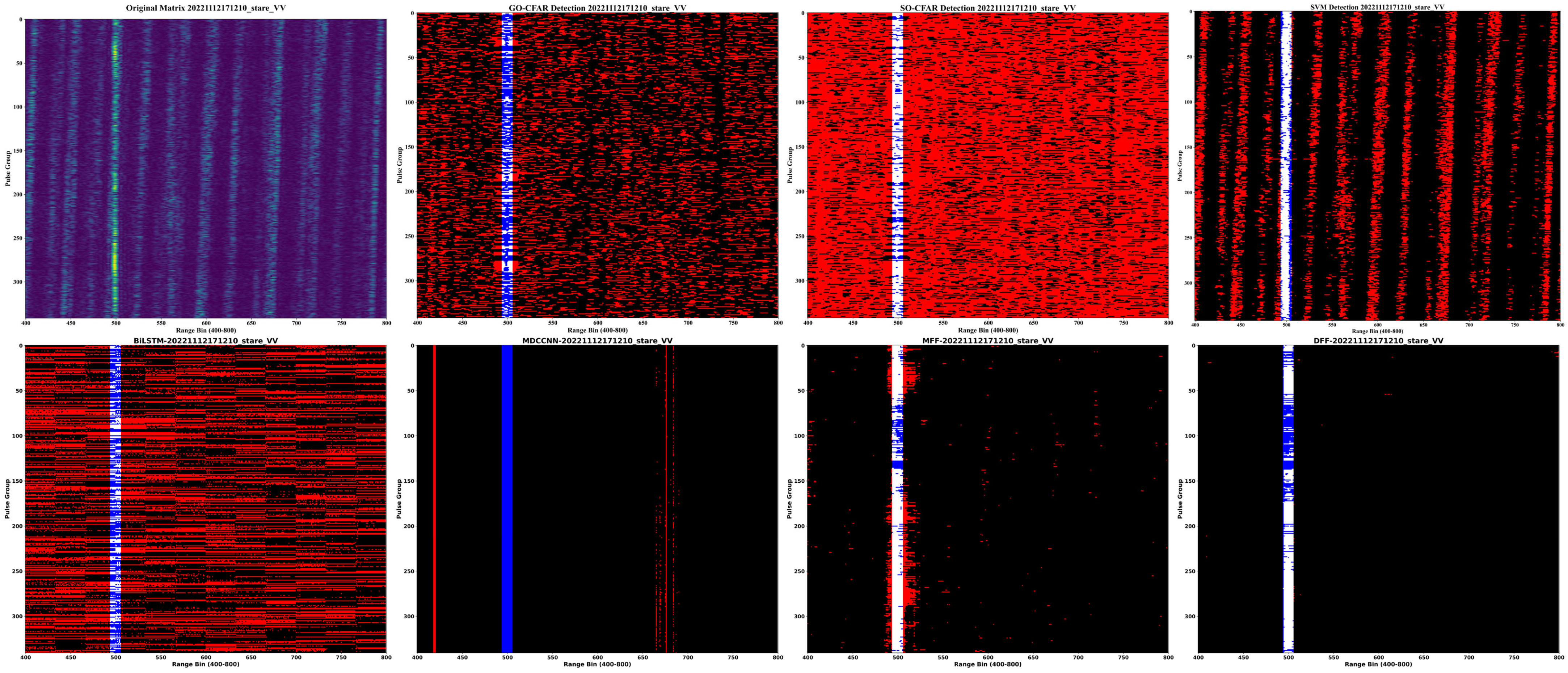
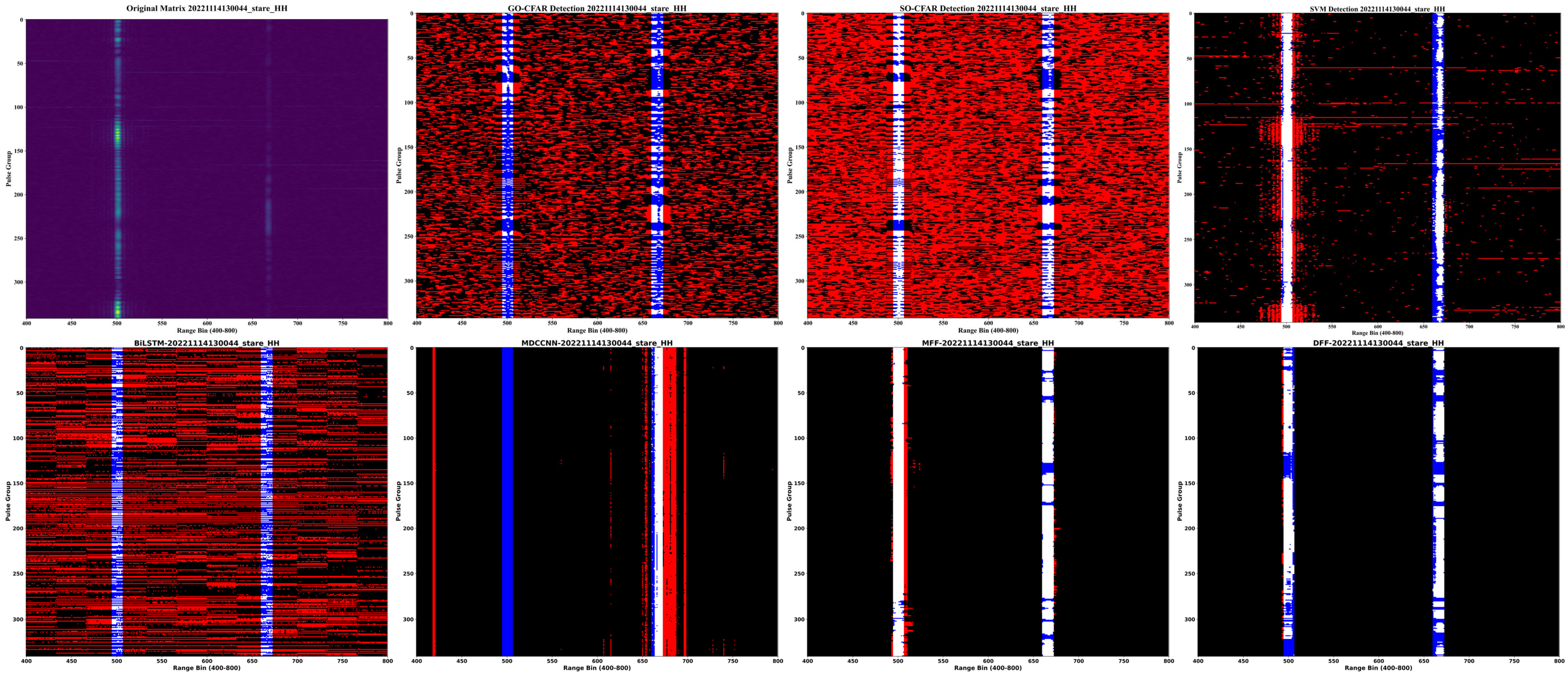
To visually characterise the detection performance of the proposed DFF detector, we further visualise the results of the seven detectors on the SDRDSP dataset. As depicted in Figure 10 and Figure 11, each visualisation classifies detection outcomes into four categories:

• Black: Regions correctly labelled as sea clutter by all methods (true negatives).
• White: Regions correctly identified as objects (true positives).
• Red: False positives (clutter regions misclassified as objects).
• Blue: False negatives (objects missed by the detectors).

The visualisations intuitively demonstrate that DFF achieves the most accurate detection, with minimal false-positive and false-negative regions. In contrast, traditional CFAR-based methods exhibit significant misclassifications to the lack of temporal context, particularly in high-clutter areas, highlighted by extensive red and blue pixels. DFF’s superior ability to suppress false alarms and retain true objects is evident from its sparse red/blue distributions, reinforcing the quantitative findings. These visual results provide intuitive evidence of DFF’s robustness in distinguishing objects from complex sea clutter, complementing the statistical analysis in Table 5.

4.3. Ablation Study

To validate the necessity of range profiles and range–Doppler maps for radar echo object detection, we designed two variant detectors of DFF: Variant model 1 employs only range–Doppler features for detection, while Variant model 2 relies solely on fast/slow time features. At a preset FAR of $1\times {10}^{-5}$, the experimental results of DFF and the two variants on the test set of the SDRDSP dataset are presented in

Table 7. Detection performance of the DFF and its variant detectors.

Name	Mean FAR	Mean Acc (%)	Mean F1 (%)
DFF	$3.5\times {10}^{-4}$	98.76	68.75
Variant model 1 a	$4.2\times {10}^{-4}$	94.63	62.83
Variant model 2 b	$4.1\times {10}^{-4}$	95.79	64.28

^a Removed the range–Doppler feature branch from DFF; ^b Removed the range–pulse feature branch from DFF.

.

The table shows that Variant 1’s $4.2\times {10}^{-4}$ FAR indicates that removing range–Doppler features reduces clutter suppression capability. Besides, DFF achieves an average FAR of $3.5\times {10}^{-4}$, which is lower than the single-source feature variants. Moreover, DFF’s average accuracy and F1-score reach 98.76% and 68.75%, respectively, outperforming the single-branch detectors in detection capability. These findings underscore the critical role of multi-modality feature fusion in enhancing object-clutter discrimination and overall detection robustness.

To demonstrate the effectiveness of our proposed multi-feature fusion method with adaptive convolutional weight learning, we compared two common feature fusion techniques in deep learning—channel-wise concatenation and element-wise summation—against our adaptive fusion module under a preset FAR of $1\times {10}^{-5}$. The experimental results of the three methods on the test set of the SDRDSP dataset are shown in

Table 8. Detection performance of different feature fusion methods.

Method	Mean FAR	Mean Acc (%)	Mean F1 (%)
Adaptive fusion (ours)	$3.5\times {10}^{-4}$	98.86	68.75
Channel-wise concation	$3.4\times {10}^{-4}$	96.43	64.87
Element-wise summation	$3.3\times {10}^{-4}$	96.74	65.42

. Unlike our approach, both baseline methods neglect the element-wise importance in feature maps, assuming uniform weights (i.e., weight = 1) for all channels or cross-source features.

As indicated in the table, while our method exhibits a slightly higher average FAR than the baselines, it significantly outperforms them in average accuracy and F1-score. This validates the effectiveness of our feature fusion method by demonstrating that AWL enhances feature discriminability, balancing detection accuracy and clutter robustness.

5. Conclusions

We draw on video-processing techniques to propose a sea-surface object detector for complex-valued data, such as sea clutter. This detector utilises range profiles and range–Doppler spectrograms to detect and track marine targets in complex sea-clutter environments. DFF introduces two key innovations: (1) native complex-valued processing to preserve phase information, and (2) joint spatiotemporal modelling through pulsed U-Net and cross-pulse SFEM. This dual mechanism significantly enhances the detection capability of marine targets in clutter-dominated environments. Extensive experiments on the public IPIX and SDRDSP datasets demonstrate that our method outperforms traditional models, including CFAR-based statistical methods and machine learning methods. The results validate the effectiveness of joint feature learning and representation in marine object detection. Due to the large memory consumption and computational latency of deep learning models in practical applications, we plan to explore improvements in the real-time performance of DFF in the future, leveraging frequency-domain processing techniques like wavelet–Fourier hybrid modules [49] to reduce computational latency and investigate encoder-free architectures like those in [50], combined with [28,49] for near-shore optical-RF fusion. Additionally, using only two types of radar echo data [34] does not allow for the detection of multiple targets in the same scene as separate instances and makes it hard to cover some specific scenarios, e.g., spikes, nearshore, etc. We also expect to explore the joint use of multi-modal data [40] in the future to achieve precise object identification versus traditional statistical models in the future.