A Novel Explainable Deep Learning Framework for Accurate Diabetes Mellitus Prediction

Abstract

Diabetes, a chronic condition caused by insufficient insulin production in the pancreas, presents significant health risks. Its increasing global prevalence necessitates the development of accurate and efficient predictive algorithms to support timely diagnosis. While recent advancements in deep learning (DL) have demonstrated potential for diabetes prediction, conventional models face limitations in handling class imbalance, capturing complex feature interactions, and providing interpretability for clinical decision-making. This paper proposes a DL framework for diabetes mellitus prediction. The framework ensures high predictive accuracy by integrating advanced preprocessing, effective class balancing, and a novel EchoceptionNet model. An analysis was conducted on a diabetes prediction dataset obtained from Kaggle, comprising nine features and 100,000 instances. The dataset is characterized by severe class imbalance, which is effectively addressed using a proximity-weighted synthetic oversampling technique, ensuring balanced class distribution. EchoceptionNet demonstrated notable performance improvements over state-of-the-art deep learning models, achieving a 4.39% increase in accuracy, 8.99% in precision, 2.19% in recall, 5.55% in F1-score, and a 7.77% in area under the curve score. Model robustness and generalizability were validated through 10-fold cross-validation, demonstrating consistent performance across diverse data splitting. To enhance clinical applicability, EchoceptionNet integrates explainable artificial intelligence techniques, Shapley additive explanations, and local interpretable model-agnostic explanations. These methods provide transparency by identifying the critical importance of features in the model’s predictions. EchoceptionNet exhibits superior predictive accuracy and ensures interpretability and reliability, making it a robust solution for accurate diabetes prediction.

1. Introduction

Diabetes, also known as “diabetes mellitus”, is a metabolic condition that grows when the pancreas cannot make enough insulin or when the body uses it badly [1]. The disorder causes either high or low blood sugar in the human body. Diabetes typically manifests in clinical situations, early-stage diabetes, and overt diabetes [2]. Several tests are used to identify the presence of diabetes, such as the glucose tolerance test that yields glucose greater than 200 mg/dL and persistent plasma glucose greater than 126 mg/dL for two or three hours [3]. Each region uses different tests based on varying blood glucose thresholds. Therefore, the use of glycemia as a diabetes evaluation metric by physicians is still under discussion [4].

Diabetes is lethal if it is not detected early or appropriately treated [5]. Patients with diabetes are at a higher risk for organ damage, which can lead to stroke, heart attack, nerve damage, kidney damage, and other complications. This situation raises the possibility that diabetes is the root cause of numerous serious diseases if it is not detected in time. According to the World Health Organization, there were 422 million cases of diabetes in the world in the year 2020, and the figure is expected to reach 490 million in the year 2030 [6]. It should be noted that the prevalence of diabetes worldwide dropped from 2000 to 2010; however, it has been steadily rising over the past decade in developing countries. The rate of mortality due to diabetes increased from 70% in 2000 to 80% in 2020. Diabetes is triggered by harmful eating habits, poor lifestyle choices, obesity, hypertension, and other conditions [7].

Detection systems based on machine learning (ML) and deep learning (DL) models have been implemented [8], and researchers have been concentrating on disease prediction so that a doctor may identify conditions such as diabetes earlier. Numerous methods and technologies have been used to predict diabetes, including multi-layered feedforward neural networks (MLFNNs) [9], deep neural networks (DNNs) [10], support vector machines (SVMs) [3], and ensemble models [11]. It is evident that this field has already begun to expand its capabilities, but its approaches have not yet reached accuracy or efficiency. Although various researchers have shown interest in predicting diseases, there is a pressing need to effectively address the threat posed by diabetes, especially given its rapid rise.

1.1. Research Gaps

• Existing studies often overlook the impact of imbalanced data distribution, which leads to biased predictions and poor generalization for minority classes in diabetes prediction tasks.
• Many current models lack the architectural depth or innovation necessary to capture complex and non-linear patterns in medical data, limiting predictive performance.
• The robustness and reliability of existing predictive models are not thoroughly validated across diverse data splits, raising concerns about their generalizability in real-world scenarios.
• Most prior research does not provide sufficient interpretability, making it difficult for healthcare professionals to trust and understand the reasoning behind the predictions.

1.2. Contributions

• We present a framework for accurate diabetes prediction that combines effective class balancing, DL, and explainability.
• As part of this framework, we address the class imbalance problem using the proximity-weighted synthetic (ProWSyn) minority oversampling technique, which enhances the model’s ability to detect underrepresented diabetic cases by generating realistic synthetic samples near decision boundaries.
• We propose a novel DL model, EchoceptionNet, which incorporates both temporal and spatial feature extraction mechanisms, enabling it to capture complex patterns in medical data more effectively than existing models.
• The robustness and generalizability of the proposed model were evaluated through 10-fold cross-validation (10-FCV), demonstrating consistent performance across various data splits.
• To ensure interpretability and clinical trust, we incorporate explainable artificial intelligence (AI) techniques Shapley additive explanations (SHAP) and local interpretable model-agnostic explanations (LIME) to provide insights into feature importance and model decision-making.

The remainder of the paper is organized as follows: Diabetes-related studies are discussed in Section 2. The proposed framework is presented in Section 3. Section 4 presents the findings of the simulation results. The paper’s conclusion and future work are discussed in Section 5. The lists of abbreviations and symbols used in this study are provided in

Table 1. List of abbreviations.

Abbreviation	Description
AI	artificial intelligence
DL	deep learning
ML	machine learning
CNN	convolutional neural network
ProWSyn	proximity-weighted minority oversampling
ResNet	residual neural network
InceptionNet	inception network
EchoceptionNet	echoception network
ESN	echo state network
LIME	local interpretable model-agnostic explanations
MLFNN	multi-Layered feedforward neural network
SHAP	Shapley additive explanations
SVM	support vector machine
10-FCV	10-fold cross-validation

and 

Table 2. List of symbols.

Symbols	Description
x	Input feature vector of the dataset.
y	Binary label indicating diabetes status (1 for diabetic, 0 for non-diabetic).
$\widehat{y}$	Predicted probability of diabetes status.
$x^{\prime }$	Synthetic sample generated using ProWSyn.
$d(x,B)$	Distance of sample x from the decision boundary B.
$\Theta$	Trainable parameters of the model.
$\lambda$	Regularization coefficient.
$h_t$	State of the reservoir at time t.
$W_{in}$, W, $W_{back}$	Trainable weight matrices for input, internal, and feedback connections in EchoceptionNet.
$F_i\left(x\right)$	Feature map for filter i.
z	Integrated feature vector combining temporal and spatial features.
$z_{fc}$	Output of the fully connected layer before final prediction.

, respectively.

2. Related Work

This section discusses some of the main works in diabetes prediction, which indicate the high efficacy of different ML and DL techniques, preprocessing methods, and feature extraction techniques. These techniques have led to higher predictive results and increased model performance. MLFNN was employed in [9] to classify the PIMA Indian Diabetes (PID) dataset. Preprocessing the dataset is an essential step for the utilized model to produce good results. In preprocessing, missing dataset values were replaced with mean values. Naive Bayes (NB) and random forest (RF), ML classifiers were used. Deep neural networks (DNNs) demonstrated excellent results when combined with the feature extraction technique on the PID dataset, with an accuracy of 98.1% [10]. Other evaluation metrics, such as specificity, sensitivity, recall, and precision, were also used because class imbalance does not significantly affect accuracy measurements. DT and RF were outperformed by the proposed model.

As DNN is primarily created for complex and multidimensional picture datasets, it is not surprising that when 1D datasets are used for testing, it produces astounding results. On a diabetic dataset obtained from the Frankfurt Hospital in Germany, researchers in [12] performed a study comparing DNN with extreme gradient boosting (XGBoost), RF, DT, SVM, and logistic regression (LR). Each technique used the grid search (GS) algorithm for adjusting hyperparameters. The proposed DNN model performed better than did decision tree (DT) and RF. In addition to DNN, convolutional neural networks (CNNs) were modified by researchers to address 1D data for enhanced disease classification and prediction. To prevent a model from performing poorly, it is crucial to handle missing values in a dataset. In [13], the authors used an outlier detection technique to deal with missing values, and to deal with the class imbalance issue, the authors used a synthetic minority oversampling technique. Deep CNN (DCNN) was used as the classification model after data cleaning and data balancing. DCNN outperformed LR, NB, SVM, classwise K-nearest neighbor (CKNN), long short-term memory (LSTM), deep belief network (DBN), and DNN, based on evaluations.

AI and the Internet of Things (IoT), along with other continuing technical breakthroughs, are steadily taking off in the world. People are content that they can instantly access every aspect of their lives, including their health, using their mobile devices. Nonetheless, there are concerns about the researchers’ capacity for logic and inventiveness. The authors in [14] developed an IoT-based diabetes monitoring solution. The model is divided into two parts. The first part is a real-time data monitoring system based on ML, mobile phone monitoring, and Bluetooth Low Energy (BLE) sensor devices. The second part is a classification system based on multi-layer perceptron, LR, and RF. An LSTM, moving average (MA), and LR-based prediction system for blood glucose levels and diabetes was developed. The model was trained and evaluated using precision and recall.

Diabetes has been linked to long-term stress, metabolic imbalance, and the autonomic nervous system, all of which have a direct impact on heart rate. Heart rate variability (HRV) changes more abruptly than do other changes in the body. In [15], the authors employed electrocardiogram HRV signals for diabetes screening. The model relied on the LSTM-CNN hybrid for feature extraction, whose output is subsequently sent to SVM for classification. The proposed model outperformed the authors’ earlier work, with a high accuracy of 95.7%. The National Health and Nutrition Examination Survey (NHNES) dataset was used in [16] to assess the effectiveness of different ML classifiers, including AdaBoost, DT, RF, and NB, coupled with LR as a feature selection method. The K2, K5, and K10 partitioning protocols were also used by the authors in the proposed work. With the combined LR-RF model, the model yielded a 94.25% accuracy on the k10 protocol. The data workload is distributed among several nodes, maximizing the use of available resources.

Another crucial element in determining a disease’s risk factor is the link between the variables in a dataset. The Bangladesh Demographic and Health Survey 2011 dataset was utilized in [17], where the authors applied the chi-square approach to assess the influence of categorical variables on one another to identify risk factors for diabetes. Different ML-based classifiers, such as SVM, RF, linear discriminant analysis (LDA), LR, K-nearest neighbor (KNN), bagged classification, and regression tree (Bagged CART), were then utilized for classification purposes. On the provided dataset, Bagged CART performed better than did the other approaches, with a high accuracy of 94.3%.

In [18], the PID dataset was utilized to predict diabetes using DT, SVM, and RF. The data was preprocessed to normalize data and eliminate outliers. GS and random search (RS) were used to adjust hyperparameters. A DL for predicting the diabetes model was put forth in [19]. To avoid over-fitting, the model adds dropout layers. Along with softmax on the output layer, other activation functions are utilized on the layers. On the diabetes type dataset and the PID dataset, the model used hyperparameters of binary cross-entropy and the adaptive learning rate method (AdaDelta). The size of healthcare datasets is growing at the same exponential rate as the global population. The study encouraged data scientists to use ML and DL techniques to achieve better outcomes. A prediction technique for the imbalanced data with missing values, named the DMP_MI model of diabetes mellitus, was introduced in [20]. For precise prediction, the model uses the NB approach to handle missing information. Thereafter, adaptive synthetic (ADASYN), a data-balancing strategy, is used to address the class-imbalance problem. In the end, RF was employed to forecast diabetes.

ML models were applied to physical examination data acquired from the Luzhou dataset in [21]. To improve model prediction, the authors employed 5-FCV. Principal component analysis (PCA) and minimum redundancy maximum relevance (mRMR) are utilized to eliminate the least important features from the data and reduce computing costs. The outcomes demonstrated that mRMR performed more effectively than did PCA. All three classifiers nearly produced identical results, but RF performed the best.

From addressing class imbalance and missing data to using hybrid models and IoT-based solutions, researchers are continuing to develop new ways to address the growing demands of precise and individualized healthcare. These studies have improved diagnostic precision and paved the way for the practical integration of predictive systems, facilitating prompt interventions and improved health outcomes. The results of these studies provide a strong foundation for future research and development of diabetes prediction models as this field advances.

Table 3. Summary of related work.

Existing Problem	Solution Proposed Previously	Weaknesses of Existing Solution	Our Propose Solution
Inadequate preprocessing and missing data handling in the PIMA Indian Diabetes dataset.	MLFNN with preprocessing techniques for removing inaccurate or missing values, surpassing NB and RF [9].	Dependency on preprocessing quality and lack of advanced DL architecture.	EchoceptionNet integrates robust preprocessing with enhanced feature learning through its dual modules.
High accuracy but limited focus on imbalanced class distributions.	DNN with feature extraction on PID dataset, achieving 98.1% accuracy [10].	Ignores class imbalance effects and relies heavily on accuracy metric.	Incorporates ProWSyn to handle class imbalance, ensuring balanced predictions for all classes.
Comparison of DNN with traditional classifiers on diabetes data.	DNN outperformed RF, DT, SVM, and XGBoost using hyperparameter tuning [12].	Focused only on DNN without addressing specific healthcare dataset challenges.	Combines temporal and spatial feature extraction for better handling of sequential healthcare data.
Handling of missing values and class imbalance in 1D datasets.	DCNN with SMOTE for data balancing and outlier detection [13].	SMOTE fails to handle complex imbalanced distributions.	ProWSyn is employed to generate realistic synthetic samples near decision boundaries.
Integration of IoT-based diabetes monitoring systems.	IoT-based real-time data monitoring and ML classification using MLP, LR, RF [14].	Limited scalability and lack of explainability in predictions.	Utilizes SHAP and LIME for explainable predictions, making results interpretable.
Link between HRV and diabetes is missing.	LSTM-CNN hybrid with SVM for HRV-based diabetes screening [15].	Focuses on HRV signals alone, limiting generalization to other datasets.	EchoceptionNet processes diverse features.
Evaluation of ML classifiers on large-scale datasets.	RF and LR combination with K-FCV [16].	Limited to traditional ML classifiers without deep learning adaptation.	Introduces advanced DL architecture tailored for complex feature interactions.
Risk factor identification in diabetes datasets.	Chi-square approach for variable correlation and classification using ML models [17].	Relies on traditional ML approaches, limiting predictive power.	Advanced feature extraction using EchoceptionNet ensures better pattern recognition.
Class imbalance and hyperparameter tuning in PID dataset.	DT, RF, and SVM with GS and RS for hyperparameter tuning [18].	Does not address the imbalance issue comprehensively.	ProWSyn ensures realistic balancing of minority classes, improving classification accuracy.
Overfitting in DL models for diabetes prediction.	DLPD model with dropout layers and AdaDelta optimizer [19].	No handling of class imbalance or explainable predictions.	Integrates ProWSyn and LIME for balanced and interpretable outcomes.
Handling missing values and class imbalance in large datasets.	DMP_MI model using NB and ADASYN, followed by RF [20].	ADASYN may generate unrealistic samples, affecting model reliability.	ProWSyn ensures proximity-based synthetic sample generation, enhancing learning.
Feature selection in healthcare datasets.	PCA and mRMR for dimensionality reduction in Luzhou dataset. [21]	Computational cost of mRMR and limited evaluation of DL models.	Utilizes advanced multiscale feature extraction in EchoceptionNet for better classification.

provides a summary of the existing work, the techniques employed in the healthcare domain, their challenges, and our proposed solution.

3. Proposed Methodology for Accurate Diabetes Prediction

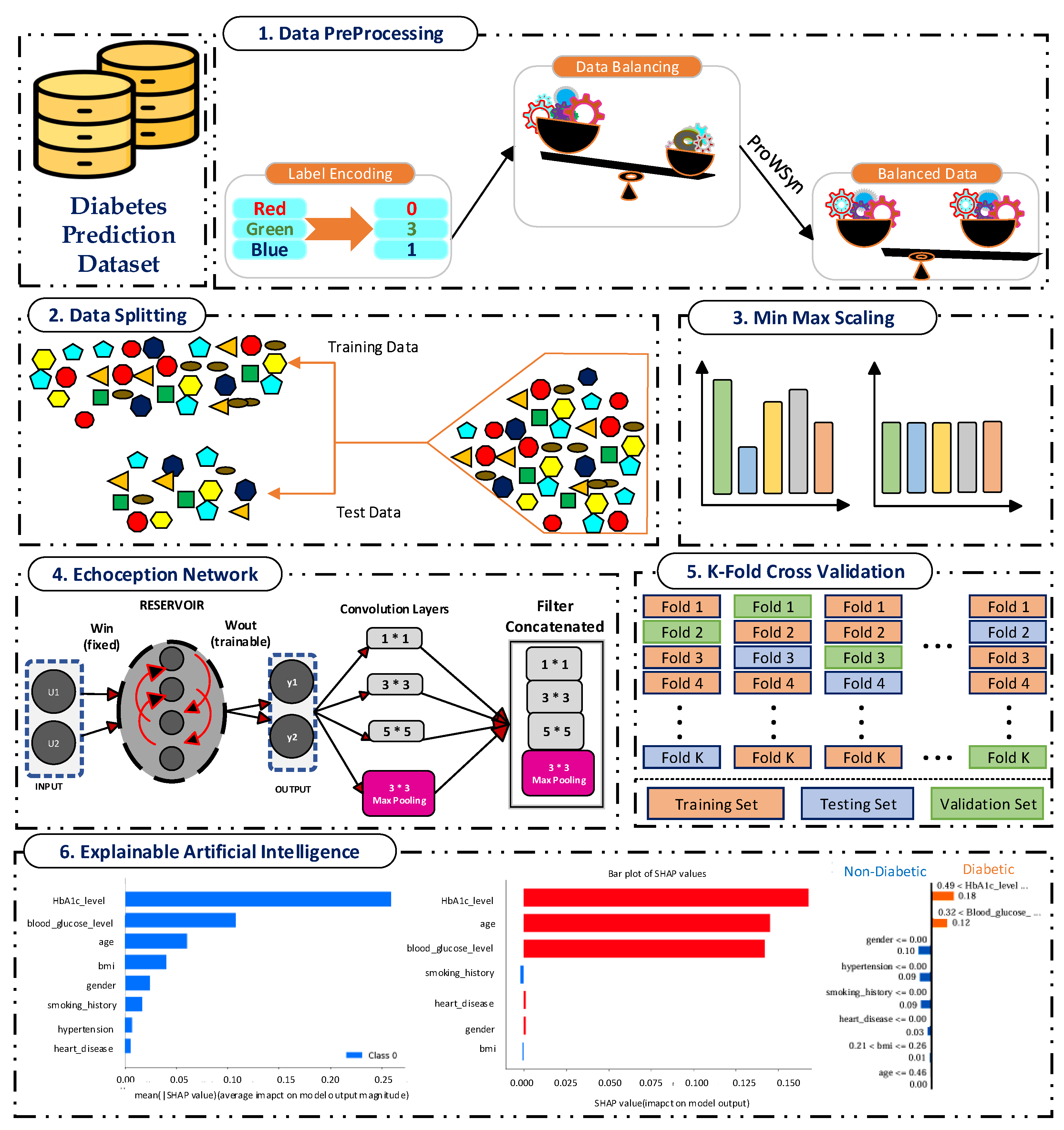
This section focuses on the elements and their interactions in the proposed system model. The proposed EchoceptionNet was developed and evaluated using Electronic Health Records (EHRs) data. This system model consists of three main components—preprocessing, balancing, and classification with EchoceptionNet—as shown in Figure 1. Together, these four elements provide a thorough system model proposed for accurate diabetes prediction. The methodology used for the proposed solution is described in

Table 4. Methodologies used in the paper.

Method	Description	Key Features	Applications
Label Encoder	Converts categorical labels into numeric values to make them suitable for DL models.	Provides efficient transformation of categorical data into numerical format.	Supports data preprocessing for classification tasks, including diabetes prediction.
Min-Max Scaler	Scales the feature values to a range between 0 and 1, improving model convergence.	Retains 99.7% of data within three standard deviations while replacing extreme outliers with boundary values.	Serves as a pre-processing step as models always require standardized input features.
ProWSyn	Generates synthetic data by considering the proximity of instances to create a balanced dataset.	Addressing class imbalance through proximity-based sampling, improving model performance on minority classes.	Facilitates the handling of class imbalance for predictive models, particularly in medical data such as diabetes prediction.
EchoceptionNet	A novel DL model designed for sequential data analysis, incorporating temporal and feature extraction capabilities.	Effective temporal feature modeling, combined with advanced feature extraction for improved prediction.	Predicting diabetes and other medical conditions by analyzing sequential and time-series data.
10-FCV	A model validation technique that divides data into 10 subsets, using each for validation and training.	Reduces overfitting and provides robust model evaluation by averaging results across different folds.	Guides in model selection and evaluation, ensuring generalizability of predictive models.
SHAP	Explains the output of DL models by attributing the prediction to individual features.	Provides transparent, interpretable explanations of model predictions using cooperative game theory.	Enhances interpretability in medical decision support systems, making predictions more understandable to clinicians.
LIME	A technique for explaining black-box DL models by approximating them locally with interpretable models.	Enables model interpretability on a case-by-case basis, especially for complex, opaque models.	Enhances trust in models for medical diagnosis, particularly for explaining predictions in diabetes detection.

.

3.1. Description of Diabetes Prediction Dataset

EHRs are the main source of the diabetes prediction dataset collected and were combined from several EHR sources to develop the diabetes prediction dataset. Inconsistencies in the dataset were eliminated with several pre-processing steps. EHRs offer a significant amount of patient data along with demographic factors. EHRs generate data that builds up over time and ultimately yields patients’ health information. The diabetes prediction dataset was used to identify healthy people and predict the possibility of diabetes. The dataset includes 9 features and 100,000 instances [22]. Along with patient information about their diabetes, the dataset also includes statistical and medical information. Features and their corresponding values in the diabetes prediction dataset are described in

Table 5. Diabetes prediction dataset description.

Feature Name	Description	Value
gender	A person’s biological sex.	Male, Female.
age	Age of an individual.	0–80.
hypertension	When the blood pressure in the arteries is consistently high.	0, 1.
heart_disease	Whether a person is suffering from heart disease or not.	0, 1.
smoking_history	If a person is smoking or not.	Not current, former, no info, current, never, and ever.
bmi	A measure of body fat based on weight and height.	10.16–71.55.
HbA1c	A person’s average blood sugar level over the previous two to three months.	3.5–9.
blood_glucose_level	The amount of blood glucose present at any given time.	80–300.
diabetes	Whether a person is diabetic or not.	0, 1.

.

3.2. Data Preprocessing

The raw data needed to be pre-processed before further use. The dataset was thoroughly examined and found to contain no missing or duplicate values, eliminating the need for imputation or data cleaning. The data were transformed from categorical to integer format using the label encoding technique. The ProWSyn data balancing approach addressed class imbalance, while min-max scaling was applied to normalize the feature ranges.

Label Encoder

In the diabetes prediction dataset, the categorical features of $gender$ and $smoking\_history$ are encoded using the label encoder technique, as DL models require numerical input and cannot process categorical data directly [23]. During label encoding, each category within a feature is assigned a unique integer, enabling the model to process categorical information. This approach ensures that the categories remain distinct. After encoding, the model can use the information located in categorical variables, enhancing the model’s decision-making capabilities.

3.3. Balancing the Highly Imbalanced Diabetes Prediction Dataset

Class imbalance has become a common problem in healthcare datasets, where samples of non-diabetic cases (majority class) outnumber diabetic cases (minority class). In the diabetes prediction dataset, there are 91,500 samples of healthy individuals and only 8500 samples of diabetic patients, indicating a significant class imbalance. This imbalance inclination for healthy people can lead to patients who are at high risk of getting diabetes to go unnoticed, which has detrimental effects on their health. To address this, we applied the ProWSyn oversampling technique, which balanced both classes by generating synthetic minority class samples, resulting in 91,500 instances in each class.

However, ProWSyn was introduced to address the drawbacks of existing oversampling techniques [24]. Most of these methods generate synthetic minority class samples by assigning weights to minority samples based on the calculated value, i.e., $\sigma$. This method assigns weights to the minority points based on their importance. If the KNNs of the minority sample x are close to the majority class, then the value of $\sigma$ will be high. As a result, the weight assigned to the minority samples will be high, i.e., the M point. On the other hand, A will have low weight due to the absence of KNNs in the vicinity of the majority class instances. Thus, $\sigma$ can be inappropriate for assigning the weight values, as it may completely remove some points from the minority class. This phenomenon proves that $\sigma$ cannot differentiate between the minority class and the majority class concerning the importance of learning. To address these limitations, the ProWSyn algorithm, a powerful oversampling technique, is used to generate weighted synthetic samples for the minority class. ProWSyn calculates the distance in the samples of the minority class to the decision boundary. The proximity-based method ensures the generation of synthetic samples in areas where the classifier is most likely to struggle with separating classes. ProWSyn operates in two main phases: proximity-based partitioning and synthetic sample generation. Each phase is carefully optimized to improve the model’s performance.

In the first phase, minority class samples are grouped based on their distance from the decision boundary. Since it is more difficult to categorize samples that are close to the decision boundary, the model needs to give more attention to them. The Euclidean distance formula in Equation (1) is used to determine the distance of each minority class sample x from the decision boundary B.

$$d(x,B)=\sqrt{{\displaystyle \sum _{i=1}^n}{(x_i-B_i)}^2},$$

(1)

where the number of features is n. The sample’s proximity to the decision boundary is indicated by the computed distance $d(x,B)$. However, the distance between each sample and the decision boundary determines which samples are grouped into proximity-based groupings. Each sample x is given a specified proximity level P to create the grouping. This ensures that there is a boundary between samples nearer the decision boundary with lower $P\left(x\right)$ and those farther away with greater $P\left(x\right)$. ProWSyn then divides the samples according to how close they are to the decision boundary. To acquire an equal distribution, it then generates synthetic samples [25]. This stage concentrates on difficult-to-learn areas, typically those close to the decision border with lower $P\left(x\right)$. Equation (2) is used to create synthetic samples $x^{\prime }$.

$$x^{\prime }=x+\alpha ·(x_k-x),$$

(2)

where $x_k$ is a KNN of x, and $\alpha$ is a random number in the range $[0,1]$. The number of synthetic samples generated for each minority sample x is determined using Equation (3).

$$N_x={\displaystyle \frac{C}{P\left(x\right)}},$$

(3)

where C is a constant, and $P\left(x\right)$ is the proximity level. This approach helps to generate more synthetic samples nearer the decision boundary for hard-to-learn instances, enabling the model to learn in relevant areas. Through proximity-based oversampling, ProWSyn enhances the sampling density of the minority class in difficult areas.

3.4. Data Splitting

In this study, 80% of the data is used for training the model, while the remaining 20% is reserved for testing. This split ensures that the model has access to a large portion of the data for learning patterns effectively, while also providing a sufficient and representative subset to evaluate its performance and generalization capability.

Min-Max Scaling

Min-max scaling is applied to normalize all features in the specific range, including age, BMI, and blood glucose level, to enhance the DL model’s performance and consistency. These features contain values that are too high compared to others, which leads to biased model training [26]. Min-max scaling transforms the data into a fixed range between 0 and 1, as demonstrated in Equation (4).

$$x^{\prime }={\displaystyle \frac{x-x_{min}}{x_{max}-x_{min}}}$$

(4)

where x represents the original feature value, $x_{min}$ is the minimum value, and $x_{max}$ is the maximum value of the feature. This process ensures that the values of the feature are scaled evenly in the specified range. With min-max scaling, the influence of features with large ranges, such as age, BMI, and blood glucose levels, is reduced. These features are weighted equally during the training process of EchoceptionNet. The normalization speeds up the convergence of EchoceptionNet and increases the accuracy of EchoceptionNet because features with different ranges will not dominate the learning process.

3.5. Newly Proposed Deep Echoception Network for Accurate Diabetes Prediction

The EchoceptionNet is a novel model developed for accurate and reliable diabetes prediction. Its architecture is centered around two core modules—temporal feature extraction and spatial feature extraction—each targeting distinct aspects of the complex patterns inherent in healthcare data. The dataset is represented as follows:

$$\begin{array}{cc}\hfill \mathcal{D}& ={\left\{({\mathbf{x}}_i,y_i)\right\}}_{i=1}^N,{\mathbf{x}}_i\in {\mathbb{R}}^d,y_i\in \{0,1\},\hfill \end{array}$$

(5)

where ${\mathbf{x}}_i=[x_1,x_2,\dots ,x_d]$ denotes the input features (e.g., age, BMI, and glucose levels), and $y_i$ represents the binary label indicating diabetes status (1 for diabetic and 0 for healthy). The goal of EchoceptionNet is to predict the outcome as follows:

$$\begin{array}{cc}\hfill {\widehat{y}}_i^{\left(t\right)}& =f_{\mathrm{EchoceptionNet}}\left({\mathbf{x}}_i\right),\hfill \end{array}$$

(6)

This can be done by minimizing the binary cross-entropy loss as follows:

$$\begin{array}{cc}\hfill \mathcal{L}(\Theta )& =-{\displaystyle \frac{1}{N}}\sum _{i=1}^N\left[y_{i}log\left({\widehat{y}}_i\right)+(1-y_i)log(1-{\widehat{y}}_i)\right],\hfill \end{array}$$

(7)

where $\Theta$ represents the trainable parameters of the model. To enhance generalization and prevent overfitting, ${\mathsf{\ell }}_2$-regularization is applied, yielding

$$\begin{array}{cc}\hfill {\mathcal{L}}_{\mathrm{reg}}& =\mathcal{L}(\Theta )+{\lambda \parallel \Theta \parallel }_2^2,\hfill \end{array}$$

(8)

where $\lambda$ is the regularization coefficient. Temporal features are extracted using a reservoir computing framework, which leverages sparsely connected neurons with fixed internal states. Unlike traditional recurrent architectures, the reservoir remains static during training, significantly reducing computational overhead. The reservoir state at time $t+1$ is updated as follows:

$$\begin{array}{cc}\hfill {\mathbf{h}}_{t+1}& =f(W_{\mathrm{in}}{\mathbf{u}}_{t+1}+W{\mathbf{h}}_t+W_{\mathrm{back}}{\mathbf{y}}_t),\hfill \end{array}$$

(9)

where $W_{\mathrm{in}}$ maps the input vector ${\mathbf{u}}_{t+1}$ to the reservoir, W governs internal reservoir connections, and $W_{\mathrm{back}}$ incorporates feedback from the output ${\mathbf{y}}_t$. The activation function $f(·)$ introduces non-linearity, enabling the encoding of complex temporal patterns. The reservoir outputs are computed as follows:

$$\begin{array}{cc}\hfill {\mathbf{y}}_{t+1}& =f_{\mathrm{out}}\left(W_{\mathrm{out}}{\mathbf{h}}_{t+1}\right),\hfill \end{array}$$

(10)

where $W_{\mathrm{out}}$ maps the reservoir states to the output. This mechanism effectively captures long-term dependencies in sequential data, such as glucose level trends over time. By maintaining sparsity in the connections, the reservoir avoids vanishing gradient problems while ensuring efficient learning of temporal dependencies.

To further elaborate, although the dataset consists of static features, we treat the input vector as a short sequence to leverage the temporal encoding capabilities of the reservoir. For example, consider a patient with age = 50, BMI = 29.5, glucose = 145, and HbA1c = 6.7, which forms the vector ${\mathbf{u}}_t=[50,29.5,145,6.7]$. This input is fed into the reservoir step by step, with each element influencing the evolving internal state ${\mathbf{h}}_t$. At each time step, the reservoir integrates current input dynamics with its prior state using the transformation ${\mathbf{h}}_{t+1}=tanh(W^{in}·{\mathbf{u}}_{t+1}+W·{\mathbf{h}}_t+W^{back}·{\mathbf{y}}_t)$. As a result, if a patient’s glucose or BMI is abnormally high, it can lead to significant fluctuations in the reservoir’s state, encoding critical non-linear associations. This ability to capture feature dependencies across pseudo-temporal steps enhances the model’s ability to detect at-risk patterns.

The second module focuses on extracting spatial patterns from the input features using a multi-scale convolutional architecture. Convolutional filters of sizes $1\times 1$, $3\times 3$, and $5\times 5$ operate on the input data to capture feature interactions at various scales. The operation is defined as follows:

$$\begin{array}{cc}\hfill F_i\left(\mathbf{x}\right)& =W_i^2\sigma \left(W_i^1\mathbf{x}\right),\hfill \end{array}$$

(11)

where $F_i\left(\mathbf{x}\right)$ represents the feature map generated by filter i, $W_i^1$ and $W_i^2$ are the convolutional weights, and $\sigma (·)$ is the activation function. The $1\times 1$ filter acts as a bottleneck layer, reducing the dimensionality of feature maps while preserving channel-wise information. The $3\times 3$ and $5\times 5$ filters capture local and broader spatial patterns, respectively, enabling the detection of intricate feature interactions such as the combined impact of age and BMI on diabetes (

Table 6. Hyperparameters utilized in Echoception network for accurate diabetes prediction.

Hyperparameter	Echoception Network Value
Batch Size	256
Learning Rate	0.001
Number of Neurons	128
Number of Epochs	30
Loss Function	Binary Cross-Entropy
Number of Filters	32, 64, 16
Kernel Sizes	1, 3, 5
Pool Size	3
Optimizer	Adam
Activation Functions	ReLU, Tanh, Sigmoid
Reservoir Sizes	50, 10

). These feature maps are concatenated:

$$\begin{array}{cc}\hfill \mathrm{Feature}\mathrm{Map}& =\mathrm{Concat}(F_1\left(\mathbf{x}\right),F_2\left(\mathbf{x}\right),F_3\left(\mathbf{x}\right)),\hfill \end{array}$$

(12)

and dimensionality is reduced using max-pooling:

$$\begin{array}{cc}\hfill \mathrm{Pooled}\mathrm{Features}& =max(F_1,F_2,F_3).\hfill \end{array}$$

(13)

The pooled features are integrated into a single feature map (

Table 7. Architecture of newly proposed Echoception network for accurate diabetes prediction.

Architecture
1. Input Layer (input shape = $(batch\_size,time\_steps,1)$)
2. RNN Layer (reservoir_size = `50’, return_sequences = True)
3. RNN Layer (reservoir_size = `10’, return_sequences = False)
4. Dense Layer (neurons = 64, activation = sigmoid)
5. Dense Layer (neurons = 32, activation = sigmoid)
6. Conv1D Layer (kernel_size = 1, filters = 32, activation = relu)
7. Conv1D Layer (kernel_size = 3, filters = 64, activation = relu, padding = same)
8. Conv1D Layer (kernel_size = 5, filters = 16, activation = relu, padding = same)
9. MaxPooling1D Layer (pool_size = 3, strides = 1, padding = same)
10. Concatenate Outputs from All Branches
11. Dense Layer (neurons = 128, activation = tanh)
12. Output Layer (neurons = 1, activation = sigmoid)

lines 6–10). This multiscale approach enhances the model’s accurate intricate pattern detection in the given data, which is beneficial from a highly specialized medical perspective. EchoceptionNet minimizes the risk of overfitting, one of the main problems in DL models. Temporal and spatial features are integrated to form a comprehensive representation of the input data and to reduce overfitting:

$$\begin{array}{cc}\hfill \mathbf{z}& =\mathrm{Concat}({\mathbf{y}}_{t+1},\mathrm{Feature}\mathrm{Map}),\hfill \end{array}$$

(14)

where ${\mathbf{y}}_{t+1}$ encapsulates temporal dependencies, and $\mathrm{Feature}\mathrm{Map}$ represents spatial patterns. This combined feature vector is passed through fully connected layers to produce intermediary representations:

$$\begin{array}{cc}\hfill {\mathbf{z}}_{\mathrm{fc}}& =W_{\mathrm{fc}}\mathbf{z}+{\mathbf{b}}_{\mathrm{fc}},\hfill \end{array}$$

(15)

where $W_{\mathrm{fc}}$ and ${\mathbf{b}}_{\mathrm{fc}}$ are trainable weights and biases. The final prediction is computed using the sigmoid activation function:

$$\begin{array}{cc}\hfill {\widehat{y}}_i& =\sigma (W_{\mathrm{final}}{\mathbf{z}}_{\mathrm{fc}}+b_{\mathrm{final}}),\hfill \end{array}$$

(16)

where $W_{\mathrm{final}}$ and $b_{\mathrm{final}}$ are trainable parameters, and $\sigma \left(z\right)={\displaystyle \frac{1}{1+e^{-z}}}$ ensures the output is a probability between 0 and 1. The reservoir module ensures the effective encoding of temporal dependencies, while the multi-scale convolutional system enhances the model’s ability to detect subtle spatial patterns. EchoceptionNet’s combination of these two modules results in a strong representation of intricate medical data while reducing dimensionality and sparsity to prevent overfitting. Additionally, replacing fully connected layers with global average pooling further reduces trainable parameters without compromising performance.

This hybrid design makes EchoceptionNet particularly suited for healthcare applications, where understanding both temporal trends (e.g., glucose fluctuations) and spatial feature interactions (e.g., BMI and HbA1c levels) is critical for reliable predictions. The step-by-step procedure of EchoceptionNet for diabetes prediction is outlined in Algorithm 1. It starts with Module 1, temporal feature extraction, although it can be modified for sequential data, as shown in Algorithm 1 (Lines 2–8). At this step, age, HbA1c level, blood sugar, and BMI are entered into the network. In this paper, we employ the reservoir framework, where the input passes through a reservoir layer. The weight matrices $W^{in}$ and W connect the inputs and internal states of the reservoirs, and the final output is given by Algorithm 1 (Lines 6–8). The reservoir state stores the dependencies and patterns from the input data and is useful for the management of sequential information in datasets.

The second module focuses on the spatial feature extraction process, as given in Algorithm 1 (Lines 9–14). This module also performs convolution with various kernel sizes, which makes the model capture different levels of abstraction or spatial arrangements within the data. Dimensionality reduction is accomplished using the $1\times 1$ contraction, and finer feature interactions are achieved using the $3\times 3$ and $5\times 5$ contractions. These feature maps are then concatenated and followed by max-pooling to combine all the learned features into one feature vector, as shown in Algorithm 1 (Lines 12–14).

In Algorithm 1 (Lines 15–17), an input from Module 1 carried out with the demographic data is concatenated with the output from Module 2 with the feature maps into the long feature vector, $X_{combined}$. The features combine with fully connected layers, which gives an intermediary output Z (refer to Algorithm 1 (Lines 18–22)). This output is passed through the activation function $\sigma$ to obtain the result of the sigmoid function that falls between 0 and 1, and the final weights $W_{final}$ and bias $b_{final}$ summation yields $\widehat{y}$, the predicted state of the test for diabetes (1 for diabetic and 0 for healthy).    

Algorithm 1: Newly proposed Echoception Network for accurate diabetes prediction

Input: Demographic features (age, HbA1c level, gender, blood sugar level, smoking history, diabetes status, heart disease, hypertension, BMI) Output: predicted diabetes status $\widehat{y}$   1: Module 1: temporal feature extraction   2: Initialize the input data vector $x=[Age,HbA1c,BloodSugar,BMI,\dots ]$   3: Compute the reservoir state for each input using the reservoir weight matrix:   4: $x_{res}(n+1)=f(W^{in}u(n+1)+W{x}_{res}\left(n\right)+W^{back}y\left(n\right))$   5: Calculate the output from the reservoir using:   6: $y(n+1)=f_{out}\left(W_{out}{x}_{res}(n+1)\right)$   7: Module 2: spatial feature extraction   8: Apply convolution filters with sizes $1\times 1$, $3\times 3$, and $5\times 5$ to input data (e.g., age, BMI, blood sugar, etc.) to extract spatial features:   9: $F(x,\left\{W_i\right\})=W_2\sigma \left(W_{1}x\right)$ 10: Concatenate the results from different filters: 11: $FeatureMap=Concat(F_1,F_2,F_3)$ 12: Apply max-pooling operation on the concatenated feature maps to reduce dimensionality: 13: $Pool=max(F_1,F_2,F_3)$ 14: Feature integration 15: Combine the spatial features from Module 2 with other demographic features from Module 1: 16: $X_{combined}=Concat(X_{demographic},FeatureMap)$ 17: Classification 18: Apply a fully connected layer to the combined features: 19: $Z=W_{fc}{X}_{combined}+b_{fc}$ 20: Apply an activation function to the output of the fully connected layer: 21: $A=\sigma \left(Z\right)$ 22: The final prediction is computed as 23: $\widehat{y}=\sigma (W_{final}A+b_{final})$ where $\widehat{y}$ is the predicted diabetes status (1 for diabetic, 0 for healthy). 24: return $\widehat{y}$ as the predicted diabetes status.

4. Simulations and Results Discussion

The simulations were conducted using Google Colab, a cloud-based platform for ML and DL research, utilizing NVIDIA Tesla K80 GPUs along with Python 3.10, TensorFlow 2.12, and PyTorch 2.0. The outcomes of the proposed EchoceptionNet model utilizing the diabetes prediction dataset are covered. The evaluation findings show that EchoceptionNet outperforms the existing DL models. The proposed model is assessed using different evaluation metrics, and their formulas are listed in

Table 8. Formulas of evaluation metrics used.

Metric	Formula
Precision	${\displaystyle \frac{TP}{TP+FP}}$
Accuracy	${\displaystyle \frac{TP+TN}{TP+TN+FP+FN}}$
Recall	${\displaystyle \frac{TP}{TP+FN}}$
F1-Score	$2\times {\displaystyle \frac{\mathrm{Precision}\times Recall}{Precision+Recall}}$
AUC-ROC	${\sum }_{i=1}^{n-1}{\displaystyle \frac{{TPR}_{i+1}+{TPR}_i}{2}}\times ({FPR}_{i+1}-{FPR}_i)$

. The qualities of the EchoceptionNet have a significant impact on its disease prediction capabilities. After prediction, the role of each feature in EchoceptionNet’s prediction is explained using the XAI techniques, SHAP and LIME. Table 6 and Table 7 present the hyperparameters and architecture, respectively, of the EchoceptionNet model.

4.1. Discussion of Newly Proposed Echoception Network Results

The proposed EchoceptionNet was compared with existing and baseline models, including the temporal convolutional network (TCN), vanilla recurrent neural network (VRNN), residual network (ResNet), LeNet, DNN, LSTM, gated recurrent unit (GRU) [27], inception network (InceptionNet), and echo state network (ESN). EchoceptionNet outperformed all these models in diabetes prediction based on all metrics, as shown in

Table 9. Performance comparison of Echoception network with existing DL models for accurate diabetes prediction.

Model	Accuracy	F1-Score	Precision	Recall	AUC	E.Time
TCN	0.78	0.80	0.72	0.90	0.82	293.9
VRNN	0.70	0.65	0.77	0.56	0.78	149.4
ResNet	0.68	0.55	0.95	0.39	0.72	215.1
LeNet	0.73	0.64	0.99	0.47	0.75	143.3
DNN	0.81	0.77	0.96	0.64	0.80	30.6
GRU	0.78	0.77	0.83	0.72	0.79	324.7
LSTM	0.77	0.60	0.53	0.70	0.54	356.3
InceptionNet	0.91	0.90	0.89	0.91	0.90	328.7
ESN	0.83	0.82	0.91	0.75	0.84	426.3
EchoceptionNet	0.95	0.95	0.97	0.93	0.97	386.1

. EchoceptionNet achieved superior performance, demonstrating its ability to handle the intricate patterns present in the dataset, with the highest accuracy of 0.95. The key strengths of EchoceptionNet lie in its ability to combine temporal feature extraction and spatial pattern detection through multi-scale convolutional operations, as shown in Table 7, Lines 2 and 3. This dual capability enables the EchoceptionNet to efficiently process complex relationships between features such as blood sugar levels, BMI, HbA1c levels, and other patient attributes. Consequently, EchoceptionNet excels at learning the intricate temporal dynamics and spatial interactions necessary for precise classification. The comparison of EchoceptionNet with existing DL models in all evaluation metrics is visualized in Figure 2. The insights behind the accuracy achieved by the baseline and proposed EchoceptionNet models are described in

Table 10. Accuracy insights of proposed EchoceptionNet and baseline DL models for diabetes prediction.

Model	Accuracy	Insights
TCN	0.78	TCN excels in sequence modeling, capturing temporal dependencies in time-series data. However, it may struggle with complex feature extraction from high-dimensional data, limiting its performance compared to more advanced models.
VRNN	0.70	VRNN is designed to handle uncertainty in sequential data, but their performance can be limited by the complexity of the data and their susceptibility to overfitting, especially with smaller datasets.
ResNet	0.68	ResNet performs well in vision-based tasks, but its architecture may not be ideal for sequential or tabular data, resulting in lower accuracy for this diabetes prediction task.
LeNet	0.73	LeNet, although an effective convolutional architecture, lacks the depth and complexity needed for more intricate data patterns found in medical prediction tasks. It struggles to achieve higher accuracy in this domain.
DNN	0.81	DNN provides powerful feature extraction and pattern recognition abilities. However, it is prone to overfitting without careful regularization, especially in complex datasets such as those in medical diagnostics.
GRU	0.78	GRU performs well for sequential data, offering advantages over vanilla RNNs in learning dependencies. While effective, it faces challenges in capturing more complex patterns compared to other deep learning models.
LSTM	0.77	LSTM can effectively model long-term dependencies in sequential data through its gated architecture. However, it tends to overfit on small datasets and lacks spatial feature modeling, reducing its performance in tabular medical prediction tasks.
InceptionNet	0.91	InceptionNet uses a multi-scale feature extraction strategy that works well for high-dimensional datasets, leading to superior performance. Its architecture is robust for extracting relevant features in complex prediction tasks such as diabetes detection.
ESN	0.83	ESN performs well with temporal data, leveraging dynamic reservoirs to capture patterns. However, ESN may be limited by the complexity of long-term dependencies in sequential data.
EchoceptionNet	0.95	EchoceptionNet, an advanced model for sequential data, significantly outperforms traditional methods by effectively combining temporal dependencies with advanced feature extraction techniques. Its superior accuracy demonstrates its ability to handle complex medical prediction tasks efficiently.

.

Our proposed EchoceptionNet performs exceptionally well, especially when addressing the class imbalance problem in diabetes detection. A notable improvement in sensitivity is demonstrated by the false-negative (FN) count, which decreased from 557 to 360 after using ProWSyn. This implies that ProWSyn enhances EchoceptionNet’s capacity to learn accurate representations of the minority class by assisting it in efficiently detecting diabetic cases with few false negatives. The key to EchoceptionNet’s success is its capacity to combine temporal and spatial feature extraction methods, enabling it to identify intricate patterns in medical data. Class imbalance is addressed by creating synthetic data, which gives the EchoceptionNet a strong performance that beats baseline models in terms of sensitivity and specificity.

Baseline models, such as InceptionNet and DNN, demonstrate advancements but still have notable drawbacks. Although InceptionNet’s FNs decreased from 1708 to 816, it still does not have a specific temporal extraction mechanism (

Table 11. Performance comparison of baseline and EchoceptionNet with and without data balancing.

Model	With ProWSyn				Without Data Balancing
	TP	TN	FP	FN	TP	TN	FP	FN
TCN	15,863	15,327	1974	3846	913	16,972	1233	718
VRNN	14,415	14,768	2419	4956	847	16,728	1473	863
ResNet	12,954	13,882	3537	6158	721	15,977	2122	1039
LeNet	12,538	14,214	3034	6673	763	16,492	1689	1092
DNN	14,878	15,837	1563	4127	942	17,428	819	752
GRU	15,226	15,574	1739	3962	1007	17,179	1048	713
LSTM	15,574	1739	15,226	3962	467	11,702	6590	1241
InceptionNet	17,494	16,757	1536	816	0	18,292	0	1708
ESN	17,062	16,926	1367	1245	989	18,205	87	719
EchoceptionNet	17,947	16,677	1616	360	1151	18,292	0	557

). This makes it less capable of capturing the sequential nature of medical data, which is essential for predicting diabetes. Despite reducing FNs from 752 to 4127 with its fully connected architecture, DNN still performed worse than did EchoceptionNet because it is unable to capture intricate feature interactions. DNN’s inability to interact with deep features makes it less appropriate for diabetes prediction, where temporal and spatial dependencies are crucial.

Even though ProWSyn improved the performance of several models including GRU, TCN, VRNN, LSTM, and ResNet, and these architectures still exhibited notable limitations. GRU showed an increase in true positives (TPs), from 713 to 15,226; however, it struggled with spatial feature learning, as it is fundamentally designed for temporal dependencies only. GRU’s architecture simplifies the LSTM by combining the forget and input gates into a single update gate, making it computationally efficient, but this simplification limits its capacity to model complex spatial patterns in tabular medical data. As a result, it yielded a relatively lower F1-score of 0.77 and a recall of 0.72 despite balanced data. Similarly, the LSTM model improved its TPs from 467 to 15,574 after ProWSyn, but exhibited a high false-positive (FP) count of 15,226 and a low true-negative (TN) count of 1739, indicating poor specificity and misclassification of non-diabetic patients. LSTM’s architecture, with separate input, forget, and output gates, allows it to retain long-term dependencies effectively. However, in this case, it failed to generalize well, possibly due to overfitting or inefficiencies in managing diverse spatial–temporal feature interactions.

Even though TCN’s TPs increased substantially from 913 to 15,863, it continued to suffer from a high FP count of 1974, highlighting its limited specificity. VRNN improves its TPs to 14,415 but also saw an increase in FPs to 2419, showing poor distinction between diabetic and non-diabetic samples. ResNet, although powerful in spatial feature extraction, recorded a high FN count of 6158 after balancing, suggesting its inability to capture temporal relationships. Likewise, LeNet only marginally increased TPs but had a high FN count of 3034, indicating that its shallow architecture struggles with complex medical data and class imbalance. EchoceptionNet is the best option for diabetes prediction because of its integrated approach to both temporal and spatial data, although ProWSyn enhances the performance of these models.

The spatial pattern detection component of the proposed EchoceptionNet model is critical in preserving the temporal dependency in the data. Several spatial features, such as insulin level changes periodically over a period, which are the most decisive signs of diabetes progression, cannot be effectively managed by conventional DL models, including DNN or GRU. To address this challenge, EchoceptionNet adopts sparse and randomly connected neurons within this module to perform temporal pattern identification without the vanishing gradients that usually affect the recurrent-based architecture, as shown in Table 7 Lines 1, 2, and 12. Meanwhile, the spatial component employs reservoir layers to capture varying degrees of feature interaction at various sizes. By addressing both local dependencies and global trends within the dataset, EchoceptionNet achieved the highest F1-score of 0.95 and a precision of 0.97, as shown in Figure 2.

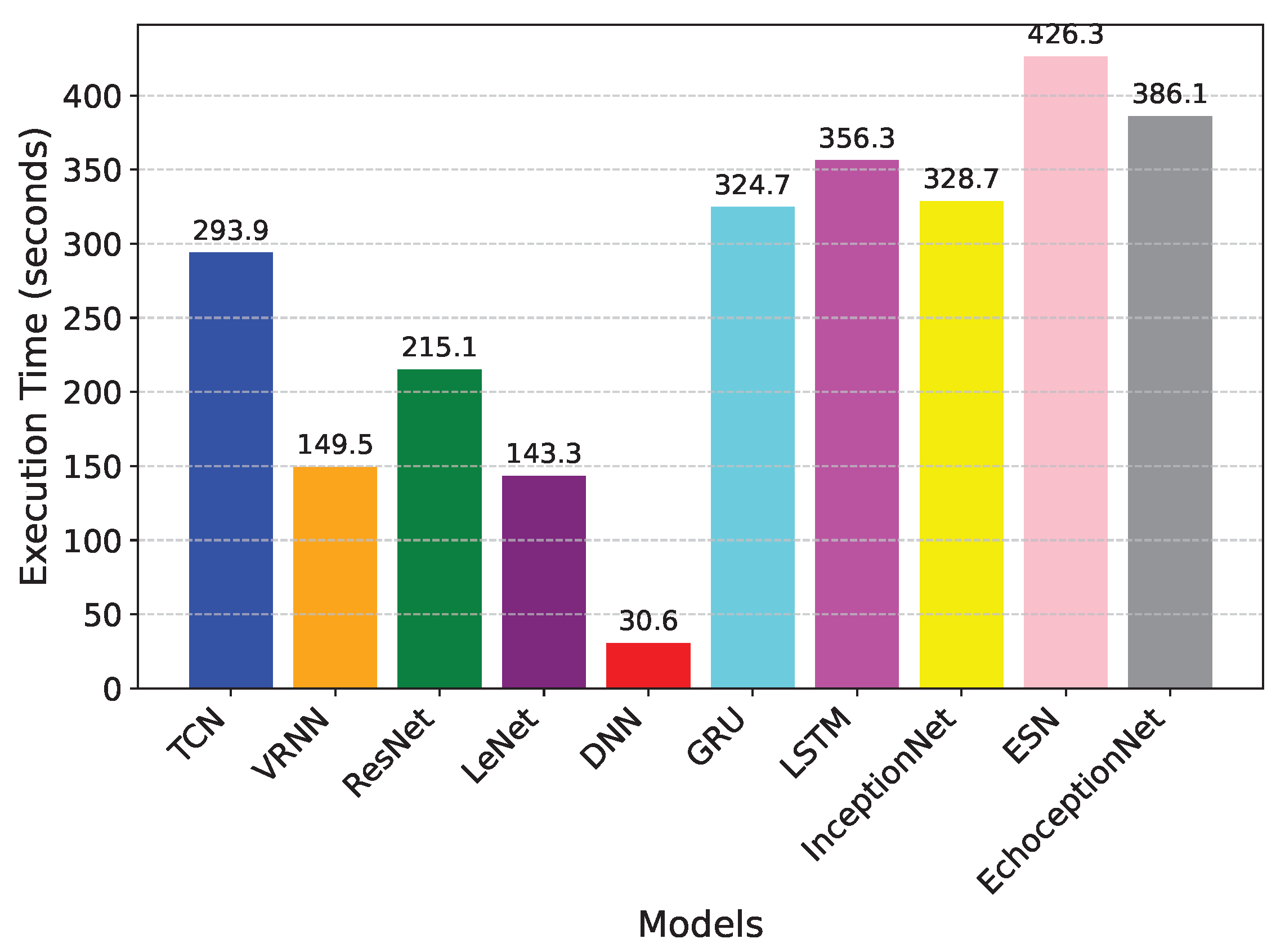
There is a noticeable difference between EchoceptionNet and InceptionNet, the model with the second-best performance. Despite achieving a commendable accuracy of 0.91, InceptionNet was unable to fully capture the sequential nature of the dataset due to its lack of temporal feature extraction, as shown in Figure 2. Its lower recall of 0.91, which indicates that it missed a larger percentage of TP cases as compared to EchoceptionNet’s recall of 0.93, reflects this weakness. The EchoceptionNet’s computational efficiency is further demonstrated by InceptionNet’s longer execution time of 328.7 s, although it has a simpler architecture than does the two-module EchoceptionNet. The execution time comparison is visualized in Figure 3.

DNN, which is employed in many classification tasks, was considerably less accurate than was EchoceptionNet, with an accuracy of 0.81. For healthcare datasets with intricate interdependencies, DNN’s generalization potential is constrained by its inability to accurately capture temporal dependencies and its dependence on fully connected layers. Its tendency to generate a high rate of FPs is highlighted by its recall of 0.64, which is especially harmful in medical applications where accurate detection is crucial. DNN’s core strength is its computational speed. This efficiency is useful in low-latency applications, but it comes at the expense of decreased predictive power, making it inappropriate for applications requiring high accuracy and dependability, such as disease prediction.

GRU also showed a relatively moderate performance, achieving an accuracy of 0.78 and a recall of 0.72. Although the GRU is specifically designed for modeling sequential data, it lacks the architectural complexity required to capture intricate spatial feature relationships, which are crucial in medical datasets such as those used for diabetes prediction. GRU simplifies the internal mechanisms of the LSTM by combining the forget and input gates into a single update gate and merging the cell and hidden states, leading to faster training and lower memory usage. However, this simplification compromises its capacity to learn deep spatial representations, resulting in a lower F1-score of 0.77 and a precision of 0.83. In contrast to LSTM, which achieved similar recall (0.70) but a significantly lower precision (0.53) and F1-score (0.60), GRU offers slightly better generalization. Nevertheless, both models fall short of the performance required for accurate diabetes classification. Additionally, the execution time of GRU was 324.7 s, which is comparable to 386.1 s of the proposed EchoceptionNet, yet the latter significantly outperformed GRU across all performance metrics, particularly with an accuracy of 0.95 and an F1-score of 0.95. This highlights the importance of integrating both spatial and temporal learning capabilities, as done in EchoceptionNet, for reliable disease prediction.

With respective accuracies of 0.68 and 0.73, ResNet and LeNet performed among the worst of the models that were evaluated. ResNet works well with image data, but it has trouble with tabular datasets because it relies too much on residual connections that are not very useful for capturing non-linear dependencies in this situation. It appears unreliable for making medical predictions due to its poor F1-score of 0.55, which further emphasizes its inability to strike a balance between recall and precision. LeNet, which was initially created for image classification, has comparable difficulties. Its 0.47 recall score, which is a result of its dependence on fixed kernel sizes and lack of temporal pattern recognition mechanisms, suggests a high rate of missed diabetic cases. Although it has a faster execution time of 143 s as compared to most models, its predictive capabilities are not adequate for practical healthcare applications.

The performance of VRNN and TCN also suggests that healthcare data is more complex and requires more refined DL models. The accuracy of the VRNN model was 0.70, while the recall was 0.56, which shows that VRNN is unable to detect diabetic cases. Similarly, TCN yielded a higher recall of 0.90 but a low precision score of 0.72, resulting in an overall accuracy of 0.78. This evidence indicates that the performance of both models puts them in a dynamic situation of compromising between sensitivity and specificity, which is a crucial measure in medical prediction.

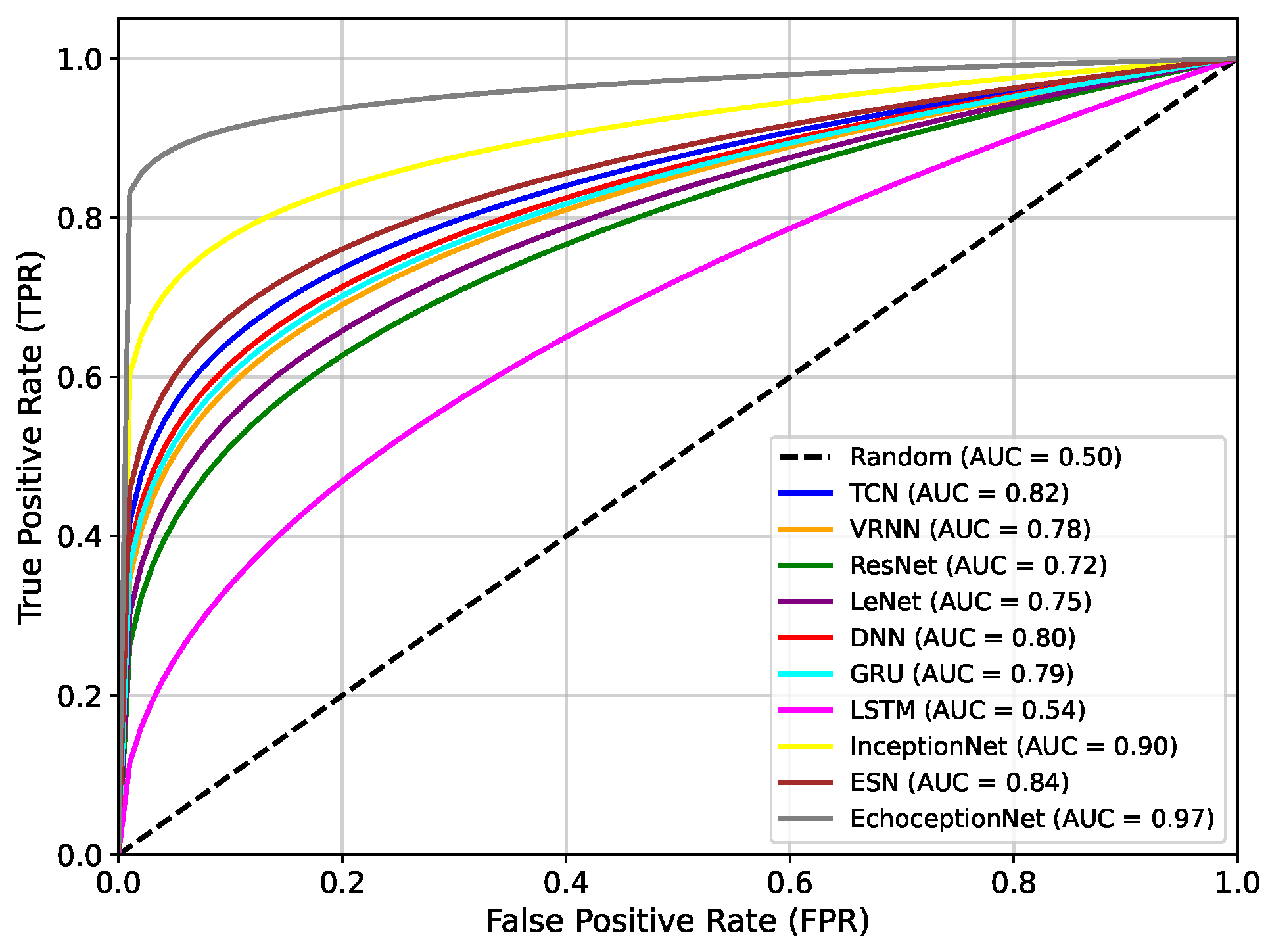
Figure 4 presents the area under the receiver operating characteristic curve (AUC-ROC) comparison of the proposed EchoceptionNet against various baseline DL models. AUC is a critical metric for evaluating a classifier’s ability to distinguish between positive (diabetic) and negative (non-diabetic) classes across all decision thresholds. Higher AUC values indicate better discrimination capabilities. The proposed EchoceptionNet achieved the highest AUC of 0.97, demonstrating superior predictive power and robustness in distinguishing diabetic patients from non-diabetic ones. This remarkable performance is attributed to its hybrid architecture that integrates both temporal and spatial feature extraction, enabling it to learn complex nonlinear patterns in the dataset effectively.

InceptionNet showed the second-best performance, with an AUC of 0.90. Although it performs well in spatial feature detection due to its multi-scale convolutional architecture, it lacks dedicated temporal modeling, which limits its sensitivity to sequential medical patterns such as blood glucose trends over time. ESN achieved an AUC of 0.84, benefiting from its reservoir-based temporal learning. However, its limited feature extraction capabilities and static internal weights hinder adaptability to complex patterns in the feature space. TCN and DNN registered AUC values of 0.82 and 0.80, respectively. TCN effectively models temporal dependencies using causal convolutions but struggles with spatial generalization. DNN, while good at static pattern recognition, lacks mechanisms for modeling temporal dynamics, limiting its ability to adapt to fluctuating patient profiles.

GRU recorded an AUC of 0.79, slightly lower than that of TCN and DNN. Its recurrent structure captures sequential data moderately well, but the absence of spatial feature modeling causes it to underperform in complex multimodal datasets.

VRNN and LeNet achieve AUCs of 0.78 and 0.75, respectively. VRNN handles uncertainty in sequences but suffers from overfitting due to its probabilistic nature. LeNet, being a shallow CNN, is inadequate for deep feature extraction in high-dimensional structured data, especially lacking both depth and temporal modeling. ResNet showed a relatively poor performance, with an AUC of 0.72. While effective in deep feature extraction, its architecture is primarily suited for image tasks and fails to adapt well to sequential tabular data. The lowest AUC was observed for green LSTM, with a value of only 0.54. Despite its powerful memory structure suitable for long-term dependencies, LSTM in this setting performs poorly due to overfitting, an excessive number of parameters, and ineffective spatial representation learning.

Overall, the steep and dominant ROC curve of EchoceptionNet validates its ability to make highly accurate predictions across different thresholds, significantly outperforming all other models in both sensitivity and specificity.

The dual-module architecture of EchoceptionNet, which synergistically integrates temporal and spatial feature extraction, is the main cause of this superiority. The temporal module aids in the model’s identification of minor temporal patterns that are crucial for the diagnosis of diabetes using reservoir layers to document sequential relationships. The spatial module simultaneously employs multi-scale convolutional filters to detect complex feature interactions that are often missed by standard DL models, such as the compounding effects of age, hypertension, and BMI. By addressing class imbalance using the ProWSyn approach, EchoceptionNet provides a balanced trade-off compared to InceptionNet, which is excellent at spatial extraction but lacks mechanisms for temporal dynamics. The proximity-based oversampling strategy, which generates synthetic data near decision boundaries, suggests that the model can better classify minority diabetic cases, as seen by its higher TP rate. To ensure convergence to a globally optimal solution without overfitting, the EchoceptionNet’s architecture is also tuned using the Adam optimizer, efficient convolutional layers, and modified hyperparameters. These features make EchoceptionNet a robust and clinically reliable model. Its steep and noticeable ROC curve shows that it can differentiate between cases with and without diabetes at all thresholds with remarkably accurate prediction.

4.2. Validating Echoception Network Results with 10-Fold Cross Validation

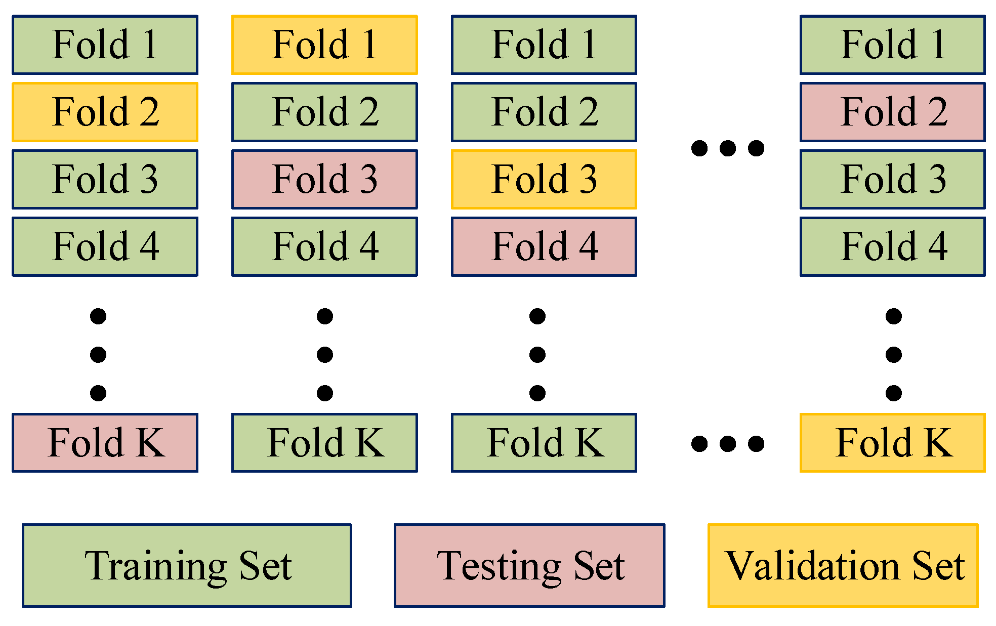
K-FCV is an effective technique used to evaluate the performance of ML or DL models when applied to different data partitions. For EchoceptionNet, the dataset is first partitioned into ten folds, where each fold is used once as the testing set, and the remaining nine folds are further split into training and validation sets. This method provides an estimate of the model’s predictive performance on unseen data, which is essential for real-world applicability and practical deployment [28]. In each iteration, eight folds are used for training, one for validation, and one for testing. In an attempt to prevent bias and volatility in the results, this procedure is repeated ten times, with each data point used for both training and testing, as shown in Figure 5.

Table 12. Ten-fold cross-validation results of proposed EchoceptionNet for accurate diabetes prediction.

Metric	1st F	2nd F	3rd F	4th F	5th F	6th F	7th F	8th F	9th F	10th F	Average
Accuracy	0.94	0.92	0.93	0.95	0.93	0.94	0.93	0.96	0.94	0.95	0.95
F1-score	0.94	0.93	0.93	0.95	0.93	0.94	0.94	0.95	0.94	0.96	0.95
Precision	0.96	0.94	0.92	0.96	0.97	0.96	0.92	0.92	0.96	0.95	0.94
Recall	0.93	0.96	0.94	0.91	0.94	0.90	0.95	0.95	0.96	0.96	0.94
E.Time	200.8	184.2	181.7	182.2	265.1	159.4	191.3	266.1	200.7	265.5	215.7

shows the 10-FCV results of EchoceptionNet, with the last column depicting the mean performance across the 10 folds. The results of EchoceptionNet were cross-validated using 10-FCV. The reliability of the model is reinforced by Table 9, which validates EchoceptionNet’s performance over multiple folds. It is important to use 10-FCV for evaluation to reduce the influence of the methodology split of data on the model. Unlike traditional methods that use a single train–test split, this approach incorporates a dedicated validation set within each fold to fine-tune model performance and avoid overfitting. In contrast, train–test splits into a single training and testing set, which can sometimes lead to biased estimates due to the uneven distribution of data. 10-FCV offers a more systematic way to evaluate the model’s performance across the many data splits that are available. This enables the reduction of the influence of random fluctuations and makes the evaluation metrics truly indicative of the potential of the proposed model. For EchoceptionNet, this is relevant since healthcare datasets often contain highly imbalanced samples, increasing the risks of biased and noisy model results.

4.3. Interpretability Using Local Interpretable Model-Agnostic Explanations

LIME is a prominent technique in explainable AI. To clarify how a black-box model arrives at a specific prediction, LIME approximates the complex model locally using a simpler, interpretable model [29]. This local interpretability is particularly valuable in the healthcare industry, where practical deployment and trustworthiness depend on an understanding of model predictions, such as diabetes prediction [30]. In the case of EchoceptionNet, LIME enhances model transparency by identifying the contributions of individual features to specific predictions. This is important as medical professionals need justifications for critical choices such as how the contribution of BMI or HbA1c levels helps to predict diabetes.

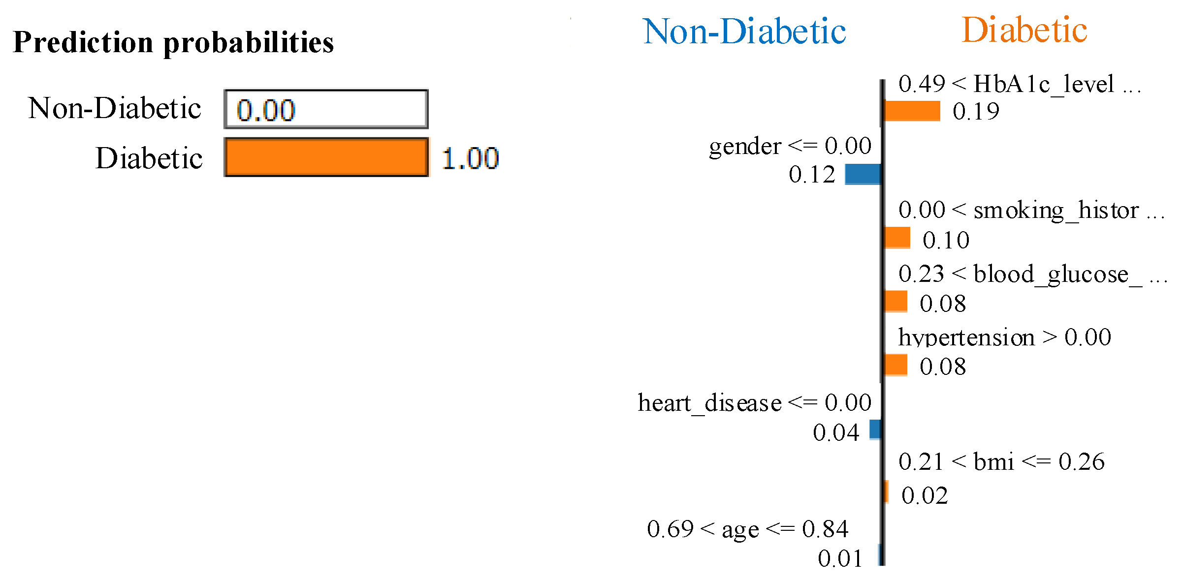
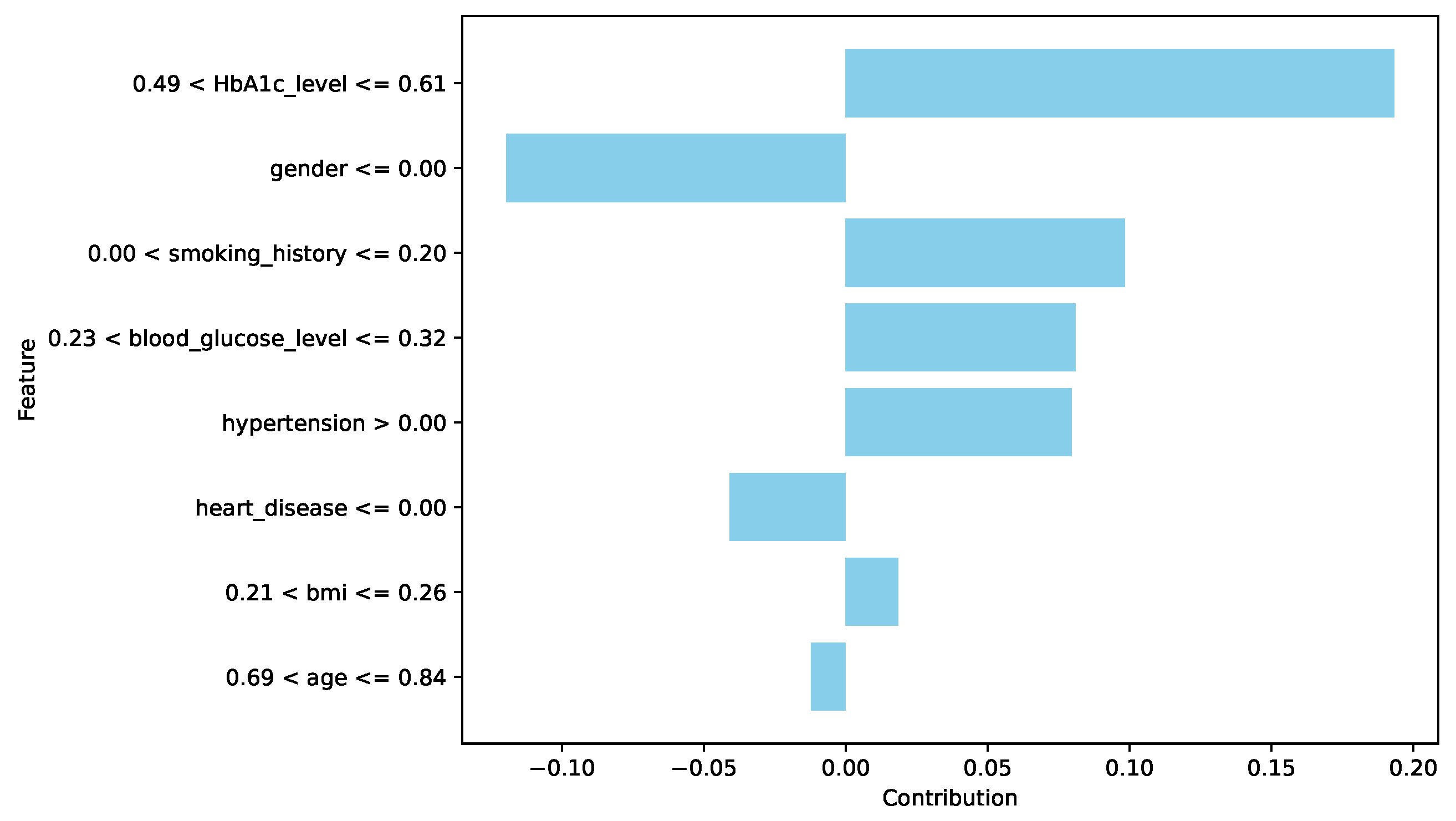
The use of LIME for the first sample is shown in Figure 6 and Figure 7. Visualizations of the probabilistic effects of features on predictions are presented, highlighting the significance of variables such as $bloodglucose,BMI$, and $HbA1c$ levels. Higher $BMI$ and $HbA1c$ values considerably skew the prediction in favor of the diabetic class, according to the histograms and summary plots in Figure 6 and Figure 7. This is consistent with medical knowledge, which holds that an elevated HbA1c is a sign of diabetes since it shows poor blood sugar control over time. The clarity of these figures is their technical advantage: it enables practitioners to see the relative contributions of each feature, such as age or hypertension, to diabetes prediction. This interpretability builds trust in EchoceptionNet by reducing the gap between clinical reasoning and AI predictions.

Similarly, Figure 8 and Figure 9 examine how features affected the 200th sample. The results support previous conclusions showing that BMI and HbA1c levels are still important predictors. Granular insights are revealed in Figure 8 and Figure 9, which highlight the small but significant contributions of secondary features such as hypertension and smoking history to EchoceptionNet’s diabetes predictions. This multi-feature analysis demonstrates the model’s resilience in capturing intricate relationships by highlighting the interdependence of diabetes risk factors. Personalized medicine relies heavily on the model’s sensitivity to individual data characteristics, which is further highlighted by the variation in feature contributions across samples.

4.4. Explainability Using Shapley Additive Explanations

SHAP is a game-theoretic approach in explainable AI that quantifies the contribution of each feature in EchoceptionNet’s predictions [31]. Since DL models often function as black boxes with limited interpretability, SHAP is employed to provide insights into the model’s decision-making process. In our implementation, background_summary is used by creating k-means clusters of 25 data points in the training set. This subset is considered a reference set to understand the importance of each feature. We utilized SHAP’s KernelExplainer, which estimates the impact of each feature by comparing model predictions for different perturbations, using background_summary as the background distribution.

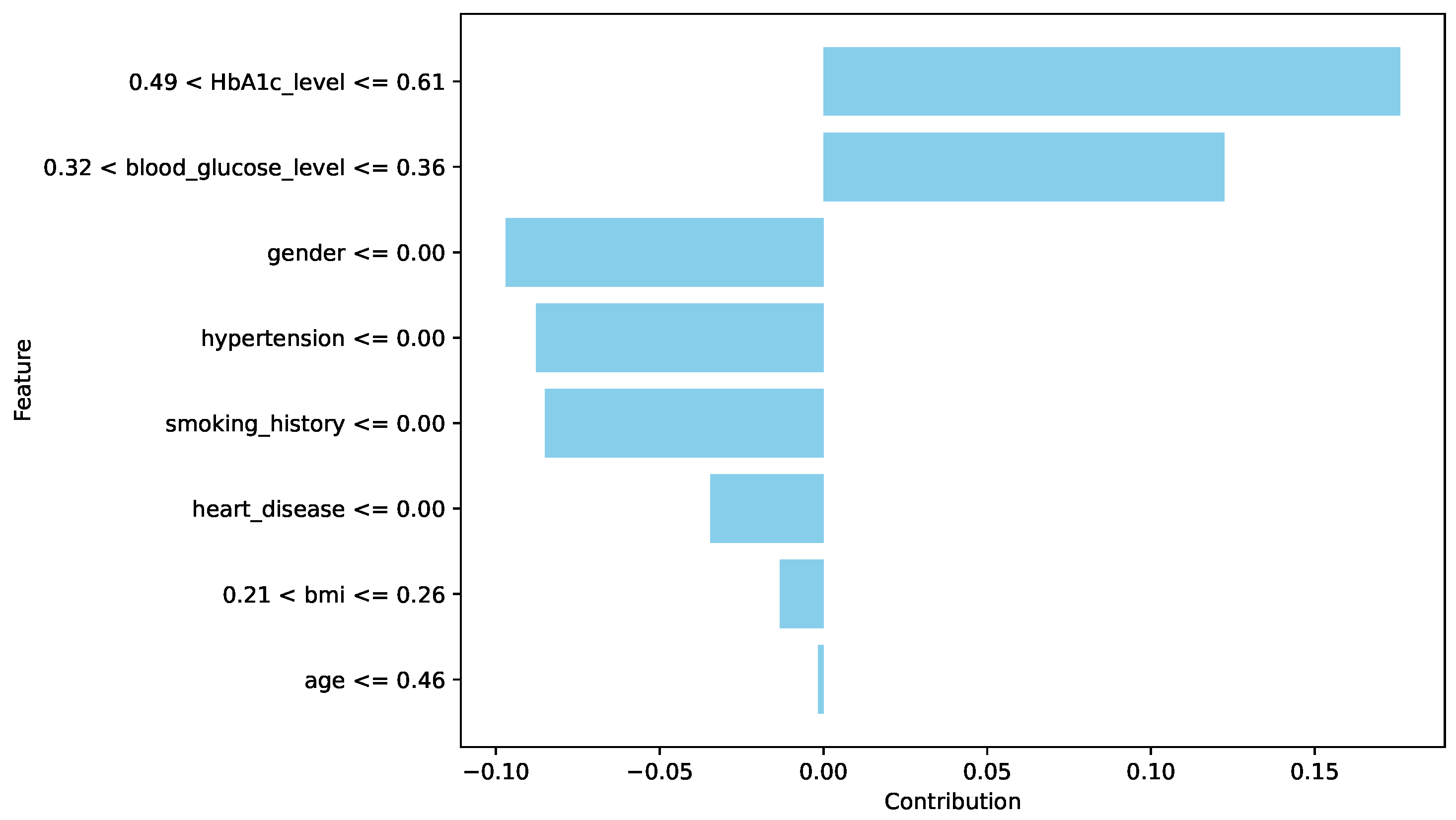
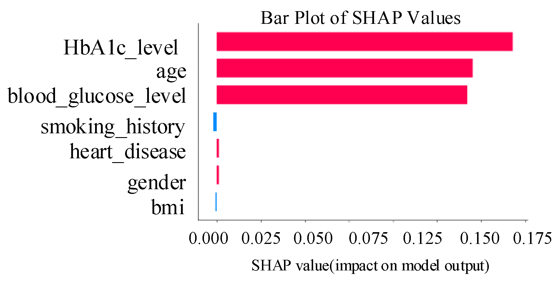
In the bar plot of Figure 10, the seven features having a positive correlation with diabetes are presented. The most important features, such as HbA1c levels, blood glucose, age, and BMI, are identified, which aligns with theoretical knowledge about diabetes. These features dominate the model’s decision-making as they offer more direct information about a particular individual’s diabetes. For example, HbA1c is one of the most important average blood glucose metrics that reflects the blood sugar level over the previous 2–3 months; logically, that it is one of the crucial predictors. Other characteristics, such as hypertension and smoking history, also show significant effects in the bar plot. These factors are not related to diabetes, but they serve as secondary predictors by identifying general tendencies related to diabetes risk. For instance, in patients, hypertension will sometimes co-occur with diabetes, enhancing its predictive capability.

The summary plot in Figure 11 shows how important each feature within the sample is and how each influences the outputs [32]. It gives a breakdown of the effect of feature values on the model’s decision whether to predict diabetes or not. In the summary plot, each bar corresponds to a particular SHAP value of the feature, while the bar indicates the extent of the feature. Additional findings include an increase in impact score, with increasing values of HbA1c level predicting diabetes. Similarly, the BMI values exhibit a similar trend, thereby supporting the clinical understanding that obesity is a key risk factor for diabetes. We can see that age or smoking history appears to have more distributed effects, which implies that these features are involved with other features in diabetes prediction.

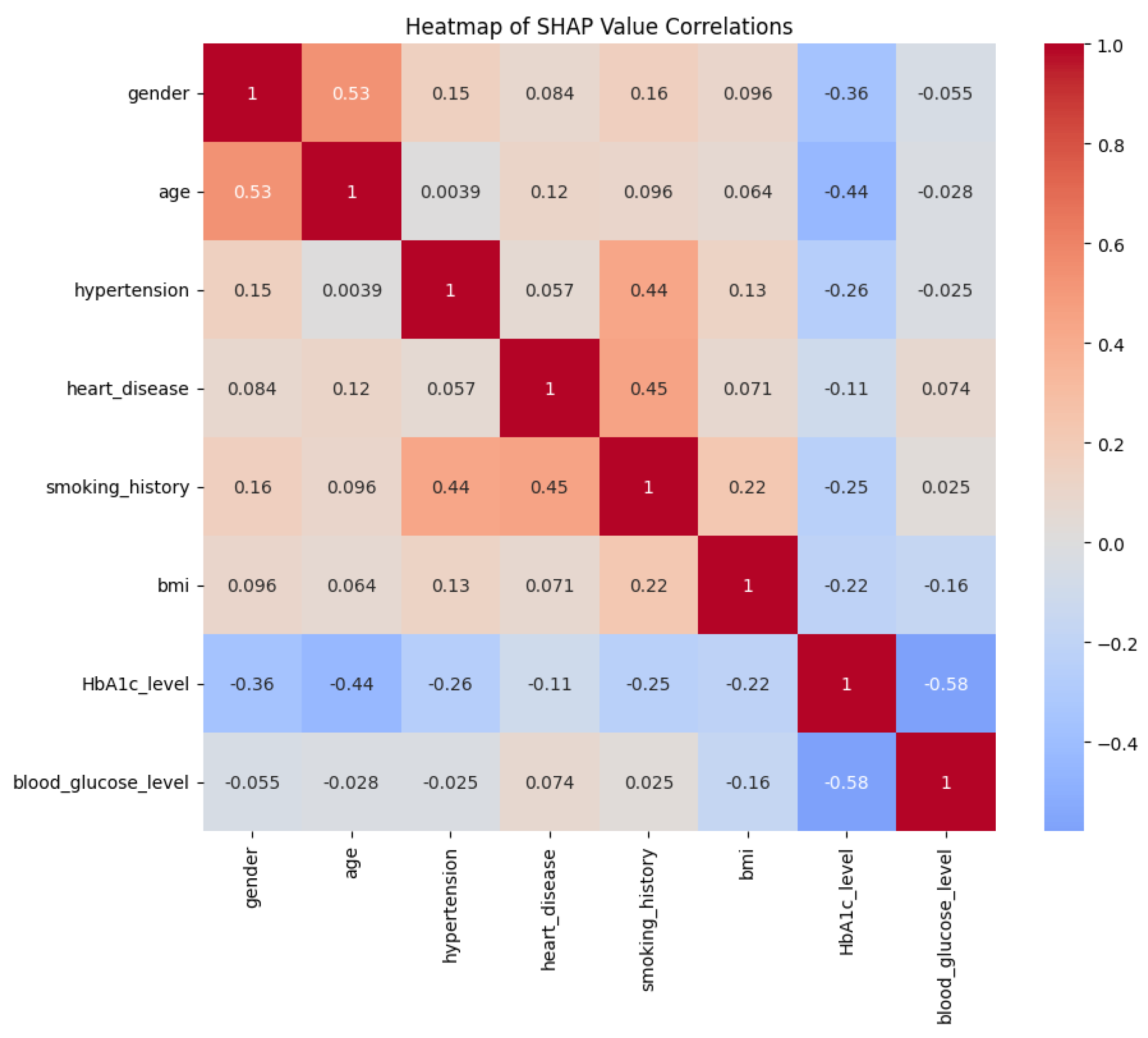
The heatmap in Figure 12 displays the general distribution of feature contributions on multiple predictions using a grid format. It helps identify regions where the model may slow down and areas where it is most effective. This is especially important for understanding how features may support predictions or diminish model projections while mapped in the spatial context. For example, heatmap analysis shows that HbA1c and blood glucose have positive contributions toward better prediction in almost all instances. However, prediction uncertainties may arise in regions with potential outliers or atypical patterns of predictor variables such as low BMI together with high blood glucose.

5. Conclusion, Limitations, and Future Work

In this study, a novel DL model, EchoceptionNet, was proposed for accurate diabetes prediction. EchoceptionNet integrates temporal feature extraction and spatial pattern detection to effectively capture complex feature interactions and temporal dependencies within the data. To mitigate the class imbalance, the ProWSyn oversampling technique was employed, enabling balanced learning and improved performance across both classes. Experimental results demonstrated that EchoceptionNet outperformed state-of-the-art DL models, achieving an accuracy of 0.95, a precision of 0.97, a recall of 0.94, and an F1-score of 0.95. To validate these findings further, 10-FCV was applied, confirming that EchoceptionNet consistently performed well across all folds. Using explainable AI techniques, such as LIME and SHAP, the decision-making process of EchoceptionNet was analyzed, revealing the significance of features, both locally and globally. These interpretations aligned closely with established clinical knowledge, reinforcing the reliability and transparency of EchoceptionNet’s predictions. With its interpretability, class-balancing capability, and robust predictive performance, EchoceptionNet provides a reliable solution for accurate diabetes prediction.

5.1. Limitations

Despite the promising results achieved by EchoceptionNet, there are a few limitations to this study that warrant further attention. First, the model was trained and validated on a static dataset from a single source, which may limit its generalizability to other populations or healthcare settings. Second, the current model framework is tailored for binary classification (diabetic vs. non-diabetic) and does not differentiate between various types or stages of diabetes. Third, the dataset lacks real-time or temporal sequence data, which limits the model’s applicability in continuous monitoring scenarios. Fourth, while SHAP and LIME were used to interpret the model’s predictions, no clinical feedback or user study was conducted to verify whether these explanations are actually useful or actionable in practice. Lastly, the model has not yet been tested in a clinical deployment environment, and factors such as integration with EHRs, user-friendliness for healthcare professionals, and interpretability under clinical constraints remain areas for future exploration.

5.2. Future Work

Future research will focus on addressing the limitations identified in this study. One direction is to evaluate EchoceptionNet on longitudinal and multi-source datasets to enhance its generalizability across different populations and clinical environments. Additionally, the model will be extended to support multi-class classification, enabling the identification of different stages and types of diabetes. Another important avenue is the integration of real-time and longitudinal health data to support continuous monitoring and early intervention. The implementation of EchoceptionNet in real-world clinical workflows, including integration with EHR systems and the development of user-friendly interfaces for healthcare providers, will also be explored. Furthermore, incorporating privacy-preserving techniques such as federated learning will be considered to ensure secure deployment in practical healthcare settings. In addition, future work will explore defining spatial relationships among demographic and clinical features based on medical domain knowledge to better inform the convolutional modeling and improve interpretability. We also plan to conduct expert reviews and user studies to evaluate the usefulness and clarity of model explanations provided by SHAP and LIME in clinical practice. Moreover, we will investigate the clinical deployment feasibility and assess runtime constraints in more detail, including response time requirements and hardware limitations, to determine the model’s suitability for real-time clinical decision support systems.

References

1. Katiyar, N.; Thakur, H.K.; Ghatak, A. Recent advancements using machine learning & deep learning approaches for diabetes detection: A systematic review. e-Prime-Advances in Electrical Engineering. Electron. Energy 2024, 9, 100661. [Google Scholar]
2. Wei, J.; Xu, Y.; Wang, H.; Niu, T.; Jiang, Y.; Shen, Y.; Su, L.; Dou, T.; Peng, Y.; Bi, L.; et al. Metadata information and fundus image fusion neural network for hyperuricemia classification in diabetes. Comput. Methods Programs Biomed. 2024, 256, 108382. [Google Scholar] [CrossRef]
3. Olisah, C.C.; Smith, L.; Smith, M. Diabetes mellitus prediction and diagnosis from a data preprocessing and machine learning perspective. Comput. Methods Programs Biomed. 2022, 220, 106773. [Google Scholar] [CrossRef] [PubMed]
4. Hasan, M.K.; Alam, M.A.; Das, D.; Hossain, E.; Hasan, M. Diabetes prediction using ensembling of different machine learning classifiers. IEEE Access 2020, 8, 76516–76531. [Google Scholar] [CrossRef]
5. Vivek Khanna, V.; Chadaga, K.; Sampathila, N.; Prabhu, S.; Chadaga, P.R.; Bhat, D.; Swathi, K.S. Explainable artificial intelligence-driven gestational diabetes mellitus prediction using clinical and laboratory markers. Cogent Eng. 2024, 11, 2330266. [Google Scholar] [CrossRef]
6. Modak, S.K.S.; Jha, V.K. Diabetes prediction model using machine learning techniques. Multimed. Tools Appl. 2024, 83, 38523–38549. [Google Scholar] [CrossRef]
7. Ahmed, N.; Ahammed, R.; Islam, M.M.; Uddin, M.A.; Akhter, A.; Talukder, M.A.; Paul, B.K. Machine learning based diabetes prediction and development of smart web application. Int. J. Cogn. Comput. Eng. 2021, 2, 229–241. [Google Scholar] [CrossRef]
8. Huang, C.C.; Kuo, W.Y.; Shen, Y.T.; Chen, C.J.; Lin, H.J.; Hsu, C.C.; Liu, C.F.; Huang, C.C. Artificial intelligence prediction of In-Hospital mortality in patients with dementia: A multi-center study. Int. J. Med. Inform. 2024, 191, 105590. [Google Scholar] [CrossRef]
9. Kumar, S.; Bhusan, B.; Singh, D.; kumar Choubey, D. Classification of diabetes using deep learning. In Proceedings of the 2020 International Conference on Communication and Signal Processing (ICCSP), Chennai, India, 28–30 July 2020; pp. 651–655. [Google Scholar]
10. Nadesh, R.K.; Arivuselvan, K. Type 2: Diabetes mellitus prediction using deep neural networks classifier. Int. J. Cogn. Comput. Eng. 2020, 1, 55–61. [Google Scholar] [CrossRef]
11. Shamsutdinova, D.; Stamate, D.; Stahl, D. Balancing accuracy and Interpretability: An R package assessing complex relationships beyond the Cox model and applications to clinical prediction. Int. J. Med. Inform. 2024, 194, 105700. [Google Scholar] [CrossRef]
12. Swapna, G.; Vinayakumar, R.; Soman, K.P. Diabetes detection using deep learning algorithms. ICT Express 2018, 4, 243–246. [Google Scholar] [CrossRef]
13. Alex, S.A.; Nayahi, J.J.V.; Shine, H.; Gopirekha, V. Deep convolutional neural network for diabetes mellitus prediction. Neural Comput. Appl. 2022, 34, 1319–1327. [Google Scholar] [CrossRef]
14. Butt, U.M.; Letchmunan, S.; Ali, M.; Hassan, F.H.; Baqir, A.; Sherazi, H.H.R. Machine learning based diabetes classification and prediction for healthcare applications. J. Healthc. Eng. 2021, 2021, 9930985. [Google Scholar] [CrossRef]
15. Madan, P.; Singh, V.; Chaudhari, V.; Albagory, Y.; Dumka, A.; Singh, R.; Gehlot, A.; Rashid, M.; Alshamrani, S.S.; AlGhamdi, A.S. An optimization-based diabetes prediction model using CNN and Bi-directional LSTM in real-time environment. Appl. Sci. 2022, 12, 3989. [Google Scholar] [CrossRef]
16. Maniruzzaman, M.; Rahman, M.J.; Ahammed, B.; Abedin, M.M. Classification and prediction of diabetes disease using machine learning paradigm. Health Inf. Sci. Syst. 2020, 8, 1–14. [Google Scholar] [CrossRef]
17. Islam, M.M.; Rahman, M.J.; Roy, D.C.; Maniruzzaman, M. Automated detection and classification of diabetes disease based on Bangladesh demographic and health survey data, 2011 using machine learning approach. Diabetes Metab. Syndr. Clin. Res. Rev. 2020, 14, 217–219. [Google Scholar] [CrossRef]
18. Ramesh, J.; Aburukba, R.; Sagahyroon, A. A remote healthcare monitoring framework for Accurate Diabetes Prediction using machine learning. Healthc. Technol. Lett. 2021, 8, 45–57. [Google Scholar] [CrossRef]
19. Zhou, H.; Myrzashova, R.; Zheng, R. Diabetes prediction model based on an enhanced deep neural network. EURASIP J. Wirel. Commun. Netw. 2020, 2020, 1–13. [Google Scholar] [CrossRef]
20. Wang, Q.; Cao, W.; Guo, J.; Ren, J.; Cheng, Y.; Davis, D.N. DMP_MI: An effective diabetes mellitus classification algorithm on imbalanced data with missing values. IEEE Access 2019, 7, 102232–102238. [Google Scholar] [CrossRef]
21. Chatrati, S.P.; Hossain, G.; Goyal, A.; Bhan, A.; Bhattacharya, S.; Gaurav, D.; Tiwari, S.M. Smart home health monitoring system for predicting type 2 diabetes and hypertension. J. King Saud-Univ.-Comput. Inf. Sci. 2022, 34, 862–870. [Google Scholar] [CrossRef]
22. Diabetes Prediction Dataset. (n.d.). Kaggle: Your Machine Learning and Data Science Community. Available online: https://www.kaggle.com/datasets/iammustafatz/diabetes-prediction-dataset (accessed on 5 August 2025).
23. Kumar, G.R.; Reddy, R.V.; Jayarathna, M.; Pughazendi, N.; Vidyullatha, S.; Reddy, P.C.S. Web application based Diabetes prediction using Machine Learning. In Proceedings of the 2023 International Conference on Advances in Computing, Communication and Applied Informatics (ACCAI), Chennai, India, 25–26 May 2023; pp. 1–7. [Google Scholar]
24. Shaheen, I.; Javaid, N.; Ali, Z.; Ahmed, I.; Khan, F.A.; Dragan, D. A transparent and robust framework for early diabetes prediction using deep residual networks and proximity-based data balancing. Biomed. Signal Process. Control 2025, 112, 108361. [Google Scholar]
25. Núñez-Vidal, E.; Fernández-Ruiz, R.; Álvarez-Marquina, A.; Hidalgo-delaGuía, I.; Garayzábal-Heinze, E.; Hristov-Kalamov, N.; Domínguez-Mateos, F.; Conde, C.; Martínez-Olalla, R. Noninvasive Deep Learning Analysis for Smith–Magenis Syndrome Classification. Appl. Sci. 2024, 14, 9747. [Google Scholar] [CrossRef]
26. Kalagotla, S.K.; Gangashetty, S.V.; Giridhar, K. A novel stacking technique for prediction of diabetes. Comput. Biol. Med. 2021, 135, 104554. [Google Scholar] [CrossRef]
27. Giancotti, R.; Bosoni, P.; Vizza, P.; Tradigo, G.; Gnasso, A.; Guzzi, P.H.; Bellazzi, R.; Irace, C.; Veltri, P. Forecasting glucose values for patients with type 1 diabetes using heart rate data. Comput. Methods Programs Biomed. 2024, 257, 108438. [Google Scholar] [CrossRef]
28. Shaheen, I.; Javaid, N.; Rahim, A.; Alrajeh, N.; Kumar, N. Empowering early predictions: A paradigm shift in diabetes risk assessment with Deep Active Learning. Knowl.-Based Syst. 2025, 315, 113284. [Google Scholar] [CrossRef]
29. Ahmed, S.; Kaiser, M.S.; Hossain, M.S.; Andersson, K. A comparative analysis of LIME and SHAP interpreters with explainable ML-based diabetes predictions. IEEE Access 2024, 13, 37370–37388. [Google Scholar] [CrossRef]
30. Lam, S.; Liu, Y.; Broers, M.; van der Vos, J.; Frasincar, F.; Boekestijn, D.; van der Knaap, F. Local interpretation of deep learning models for Aspect-Based Sentiment Analysis. Eng. Appl. Artif. Intell. 2025, 143, 109947. [Google Scholar] [CrossRef]
31. Khan, H.; Javaid, N.; Bashir, T.; Ali, Z.; Khan, F.A.; Pamucar, D. A novel deep gated network model for explainable diabetes mellitus prediction at early stages. Knowl.-Based Syst. 2025, 328, 114178. [Google Scholar] [CrossRef]
32. Ekanayake, I.U.; Meddage, D.P.P.; Rathnayake, U. A novel approach to explain the black-box nature of machine learning in compressive strength predictions of concrete using Shapley additive explanations (SHAP). Case Stud. Constr. Mater. 2022, 16, e01059. [Google Scholar] [CrossRef]
Figure 1. Newly proposed Echoception Network for accurate diabetes prediction.
Applsci 15 09162 g001
Figure 2. Performance comparison of proposed Echoception network with baseline DL models for accurate diabetes prediction.
Applsci 15 09162 g002
Figure 3. Execution time of proposed EchoceptionNet for accurate diabetes prediction.
Applsci 15 09162 g003
Figure 4. AUC-ROC comparison of proposed EchoceptionNet with existing DL models for accurate diabetes prediction.
Applsci 15 09162 g004
Figure 5. Architecture of K-FCV for the proposed Echoception network.
Applsci 15 09162 g005
Figure 6. Impact of each feature on the 1st sample illustrated by LIME. Orange bars indicate features pushing the prediction toward the diabetic class, while blue bars push it toward the non-diabetic class. Bar length reflects the strength of each feature’s contribution.
Applsci 15 09162 g006
Figure 7. Summary plot for the 1st sample by LIME. Left-side blue bars indicate negative influence toward diabetes, while right-side blue bars indicate positive influence toward the non-diabetic prediction. Bar length represents contribution strength.
Applsci 15 09162 g007
Figure 8. Impact of each feature on the 200th sample illustrated by LIME. Orange bars indicate features pushing the prediction toward the diabetic class, while blue bars push it toward the non-diabetic class. Bar length reflects the strength of each feature’s contribution.
Applsci 15 09162 g008
Figure 9. Summary plot for the 200th sample by LIME. Left-side blue bars indicate negative influence toward diabetes, while right-side blue bars indicate positive influence toward the non-diabetic prediction. Bar length represents contribution strength.
Applsci 15 09162 g009
Figure 10. Bar plot of EchoceptionNet feature contributions. Red bars indicate positive influence toward the diabetic class, while blue bars indicate negative influence.
Applsci 15 09162 g010
Figure 11. Summary plot of EchoceptionNet. All blue bars represent features contributing toward the non-diabetic (class 0) prediction. Bar length indicates the strength of each feature’s negative influence.
Applsci 15 09162 g011
Figure 12. Heatmap of EchoceptionNet feature contributions. Color intensity represents the magnitude of each feature’s influence on the model’s prediction, with darker shades indicating stronger impact.
Applsci 15 09162 g012