Unraveling Electrochemical–Thermal Synergy in Lithium-Ion Batteries: A Predictive Framework Based on 3D Modeling and SVAR

Abstract

Energy shortage and environmental pollution have accelerated the adoption of lithium-ion batteries (LIBs) as efficient energy storage solutions. However, their performance and safety challenges under extreme temperatures highlight the urgent need for effective temperature control during charging and discharging, making a comprehensive understanding of electrochemical and thermal behaviors crucial. This paper develops a 3D electrochemical–thermal coupled model for 150 Ah lithium iron phosphate (LFP) batteries to investigate thermal behavior at varying charge–discharge rates. An integrated learning regression prediction system, incorporating a structured vector autoregression (SVAR) model, is subsequently proposed to analyze the interactions among multiple electrochemical and thermal variables. The temperature difference exceeds 5 °C at higher charging rates (1.3C, 1.5C), driven primarily by accelerated heat generation—especially reversible heat. Complex interactions exist between electrochemical and thermal parameters. When charging at 0.5C, voltage, current density, battery capacity, and the maximum temperature difference (MTD) are all significantly and positively correlated (p < 0.001). Under 1C discharge conditions, voltage exhibits a strong positive correlation with most thermal characteristic variables, and correlation coefficients across different operating conditions range from −0.9731 to 0.973. Finally, the proposed ensemble learning system exhibits excellent prediction accuracy, strong generalization, and robust trend analysis, with practical guiding value.

1. Introduction

Energy shortage and environmental pollution represent some of the most formidable global challenges. The exploration of new energy technologies and the formulation of environmental protection strategies have become pivotal for promoting sustainable development [1]. Lithium-ion battery technology, as an efficient energy storage means, is actively intervening to address the dual predicaments of energy shortage and environmental protection [2]. However, the performance and capacity of lithium-ion batteries (LIBs) are impaired under low- and high-temperature conditions [3,4], so the safety of LIBs during use remains a concern among the public. The electrochemical and thermal performance of LIBs is influenced not only by their physical parameters and electrode material properties but also by the battery’s operating temperature, internal temperature uniformity, and fast charging/discharging performance [5,6]. During charge/discharge cycles, excessive temperature rise and non-uniform temperature distribution can undermine the battery’s stability [7], potentially triggering thermal runaway (TR) and posing serious safety risks. The thermal management of LIBs is regarded as one of the core challenges in its technological advancement [2]. The heat generation in LIBs mainly stems from the exothermic electrochemical reactions and the internal heat transfer processes. Therefore, an in-depth investigation of the electrochemical behavior and thermal characteristics of LIBs is of great necessity. Compared with experimental studies, simulation techniques offer a more precise and profound way to understand the thermodynamic characteristics during electrochemical reactions [8,9].

Numerous scholars have used simulation methods to conduct detailed analyses and research on the electrothermal coupling characteristics of LIBs. Doyle et al. [10] laid the foundation for the simulation modeling of LIBs. As one of the early pioneers to use the pseudo-two-dimensional (P2D) model combined with concentrated solution theory, they accurately modeled the constant-current charge/discharge behavior of lithium anodes, solid polymer diaphragms, and insertion cathode batteries. The model considered battery kinetics and thermodynamics but did not account for heat generation and dissipation during charge/discharge cycles, thus limiting the study of battery thermal behavior. Therefore, it is imperative to study the electrochemical–thermal coupling model of batteries. Mei et al. [11] combined the classic P2D electrochemical model and a three-dimensional thermal model to establish an electrochemical–thermal coupling model to simulate the internal temperature distribution of the battery and study the impact of electrode design parameters on battery performance. Nie et al. [12] used the P2D model combined with a two-dimensional thermal model to simulate the internal electrochemical reactions and heat transfer processes, studied the thermal behavior of three commercial LIBs during charge and discharge, and verified the model’s accuracy and reliability through experiments. One-dimensional and two-dimensional (1D and 2D) models have acceptable accuracy in describing the average battery temperature but are evidently insufficient in describing battery temperature distribution and temperature differences [13]. Most commercial or non-commercial electrochemical–thermal coupling models use the P2D model to simulate the heat generated by battery electrochemical kinetics [14,15] and then input the simulated heat into 2D or 3D models for calculation to obtain the temperature distribution [16,17]. However, this approach often neglects the non-uniformity of battery heat generation and the heat exchange between battery structures [18]. In contrast, 3D models perform better in this regard [19]. Bayatinejad et al. [20] established a 20 Ah 3D electrochemical–thermal model, studied the electrochemical–thermal behavior of LIBs at different discharge rates, and explored methods to improve battery performance by changing the battery’s geometric structure and current collector position. They found that changing the geometric structure could significantly enhance the uniformity of 20 Ah battery parameters and reduce the maximum surface temperature. Li et al. [21] established a 30 Ah 3D electrochemical–thermal coupling model to simulate and analyze the internal electrochemical processes and thermal characteristics of large LIBs under different discharge rates, battery thicknesses, and heat dissipation coefficients. They found that increasing the battery thickness led to an increase in the internal temperature gradient and thermal non-uniformity of the 30 Ah battery. The above studies focused only on small-capacity LIBs. However, large-capacity energy storage has become a trend, and recent research has revealed that under adiabatic conditions, the charge–discharge rate of large-capacity LIBs has a significant impact on the battery’s heat generation rate [22], Therefore, it is particularly necessary to conduct in-depth research on the thermal variation laws of large-capacity LIBs at different charge–discharge rates. Intelligent optimization algorithms, by simulating various existing phenomena, have been applied in various fields of LIBs. Wang et al. [23] proposed an improved GA-ACO-BPNN optimization algorithm for predicting the remaining useful life of LIBs. The research results showed that this algorithm has strong robustness and engineering application value in detecting and warning of the remaining useful life of LIBs. An et al. [24] developed a new decomposition genetic algorithm to solve the optimization problem of a large number of parameters in the equivalent circuit model of LIBs. The results showed that the newly developed decomposition genetic algorithm has high accuracy in multi-variable optimization. Zhu et al. [25] proposed a hybrid kernel least squares support vector regression prediction model based on variational mode decomposition and improved dung beetle optimization for the high-precision prediction of the state of health (SOH) of LIBs. They found that the determination coefficient of the model for predicting six battery health states was higher than 0.98388, verifying its high accuracy and effectiveness in predicting the SOH of LIBs. In the field of LIBs, research on out-of-condition data extrapolation prediction based on intelligent algorithms is relatively scarce.

In the research field of battery electrochemical–thermal coupling models, a large number of studies have used the P2D model, mainly focusing on the impact of changes in the geometric structure (such as height, width, and stack thickness) of small-capacity batteries on temperature distribution and cooling effects. Currently, there is relatively little research on the extrapolation of operating condition parameters of large-capacity LIBs at different charge–discharge rates based on intelligent algorithms. Most existing research focuses on battery life prediction [23,26], parameter optimization [27,28], and SOH estimation [25,29]. etc. Although existing research has used intelligent algorithms to model and optimize battery performance, there is still a significant gap in the extrapolation prediction of parameters beyond actual operating conditions. This paper constructs a 150 Ah 3D lithium iron phosphate (LFP) battery electrochemical–thermal coupling model to simulate the thermal behavior of LIBs during charge/discharge cycles. The structural vector autoregression (SVAR) model is employed to explore dynamic interactions between multiple electrochemical and temperature variables, clarifying their relative significance in the system. To reduce time costs for SVAR simulation data acquisition, an integrated learning regression prediction system is proposed. By integrating multiple advanced machine learning models, it accurately predicts key parameters (max temp difference, average temp, uniformity index) for LIBs, significantly saving calculation time and enhancing research efficiency. Through comprehensive judgment of the battery temperature distribution characteristics, it is expected to provide theoretical support for the electrochemical–thermal coupling research of LIBs.

2. Model Development and Validation

2.1. Model Assumptions

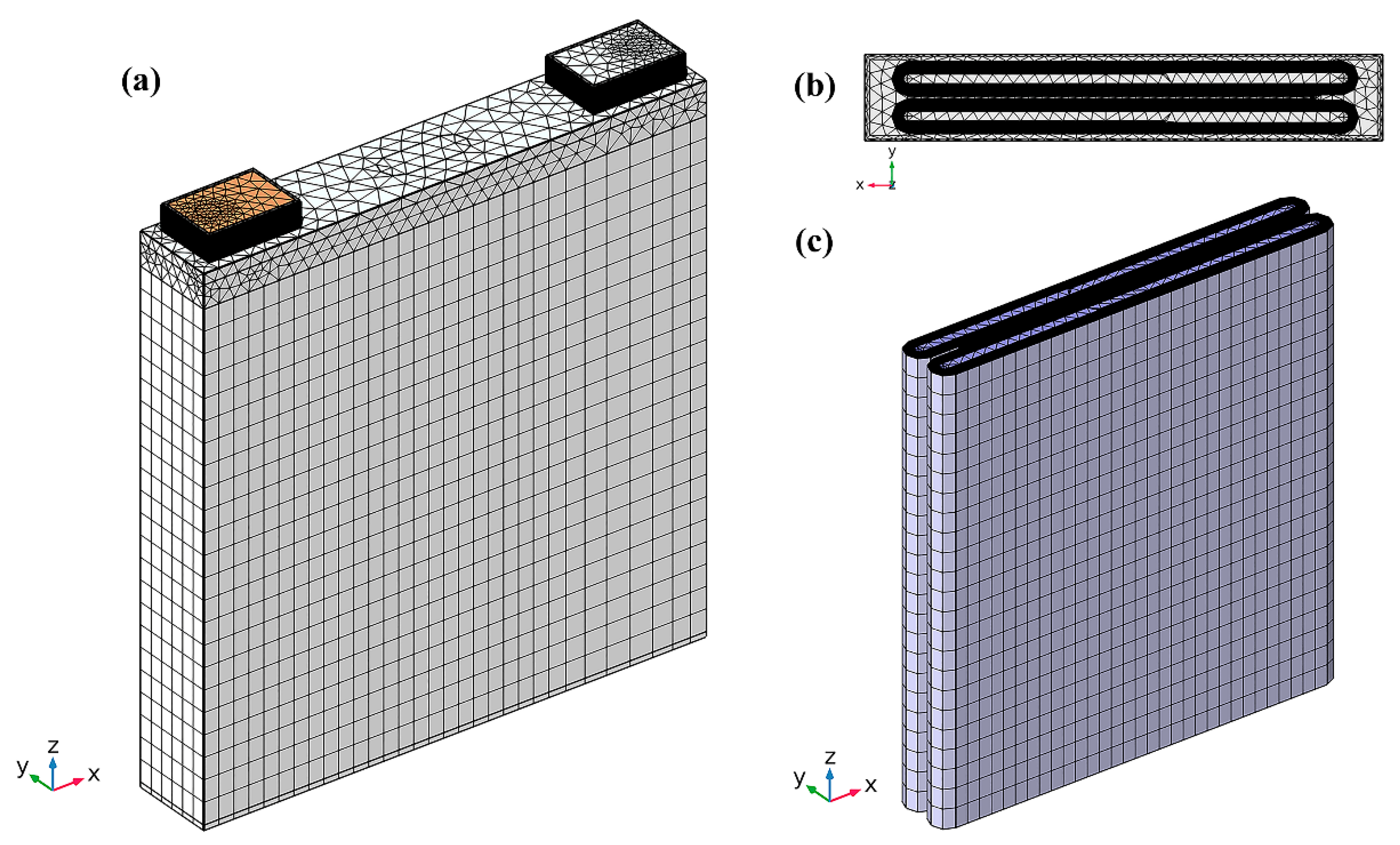
This study develops a model based on Newman’s framework [30], using a 150 Ah prismatic LiFePO₄ battery from Contemporary Amperex Technology Co., Limited (CATL), a company located in Ningde City, Fujian Province, China. The model is constructed with precise dimensions and meshed according to actual component layouts. Building upon the P2D model, this research extends charge transport, Li⁺ diffusion, and heat transfer processes into three dimensions. Boundary conditions are defined based on real-world operating environments, resulting in a 3D electrochemical–thermal coupling model for prismatic Li-ion batteries. The structure and chemical equilibrium during charge/discharge cycles [31] are shown in Figure 1. In this paper, X, Y, and Z directions correspond to the battery’s width, thickness, and height, respectively. In Figure 1b, the multi-unit domain features an adiabatic boundary on the left (internal battery) and a convective heat transfer boundary on the right (outer surface in contact with air). Figure 1c depicts a single computational unit with identical electrochemical boundary conditions across all units. The model adheres to the following principles to ensure validity [32,33]:

(1)

The particles of the active electrode material are uniformly sized spheres.

(2)

The volume change of the electrodes during the charging and discharging processes is ignored.

(3)

All side reactions between the solid, the electrolyte, and the separator are ignored.

(4)

The current collector has high electrical conductivity.

(5)

The heat generation of the current collector is ignored.

(6)

The gases that may be generated during the charging and discharging processes are ignored.

(7)

The electrodes, current collectors, separators, and electrolytes are regarded as superimposed continua.

Figure 1. (a) An electrochemical–thermal coupling model diagram of the battery. (b) A schematic diagram of the battery lamination in the multi-unit computational domain. (c) A schematic diagram of the electrochemical reaction of the battery in a single-unit computational domain.

Figure 1. (a) An electrochemical–thermal coupling model diagram of the battery. (b) A schematic diagram of the battery lamination in the multi-unit computational domain. (c) A schematic diagram of the electrochemical reaction of the battery in a single-unit computational domain.

The charging and discharging processes of LIBs involve multiple complex physical fields such as ion movement, charge transfer, and heat transfer. Based on equations such as mass conservation, charge conservation, electrochemical kinetics, and electrode kinetics, this paper establishes the physical field of heat conduction, the chemical physical field, and the electrochemical–thermal coupling physical field of a prismatic lithium-ion battery cell. It also uses intelligent algorithms to assist in analyzing the electrothermal characteristics of LIBs during the charging and discharging processes.

2.2. Electrochemical Model

2.2.1. Mass Conservation

During the charging and discharging processes of LIBs, mass conservation mainly refers to the migration of lithium ions (Li⁺) between the positive and negative electrodes of the battery. As shown in Figure 1c, during charging, Li⁺ migrate from the positive electrode to the negative electrode, and during discharging, Li⁺ migrate from the negative electrode to the positive electrode. The migration of Li⁺ is achieved through the electrolyte [33]. Therefore, the mass conservation during the charging and discharging processes of LIBs involves three aspects: the solid phase, the liquid phase, and the electrochemical kinetics of Li⁺.

When Li⁺ are deintercalated from the solid-phase electrode, the mass conservation between Li⁺ and the active substances of the solid-phase electrode follows Fick’s law, as defined by Equation (1) [5,34]:

$${\displaystyle \frac{\partial c_{{\mathrm{L}\mathrm{i}}^{+},s}}{\partial t}}-{\displaystyle \frac{D_{{\mathrm{L}\mathrm{i}}^{+},s}}{r^2}}{\displaystyle \frac{\partial }{\partial r}}\left(r^2{\displaystyle \frac{\partial c_{{\mathrm{L}\mathrm{i}}^{+},s}}{\partial r}}\right)=0$$

(1)

where c_Li⁺_,s is the concentration of Li⁺ in the spherical active particles in the solid phase, mol/m³; t is the time, s; D_Li⁺_,s is the diffusion coefficient of Li⁺ in the spherical active particles in the solid phase, m²/s; r is the particle radius of the spherical active particles, µm.

After Li⁺ are deintercalated from the solid-phase electrode and migrate to the other electrode through the electrolyte, the mass conservation of Li⁺ in the electrolyte follows Equation (2) [35].

$${\epsilon }_e{\displaystyle \frac{\partial c_{{\mathrm{L}\mathrm{i}}^{+},e}}{\partial t}}=\nabla ·\left(D_e^{eff}\nabla c_e\right)+{\displaystyle \frac{{\mathrm{a}}_{sap}{J}_{lcd}}{F}}(1-t_{+})$$

(2)

After the homogenization treatment of the porous electrode, the diffusion coefficient of Li⁺ in the electrolyte needs to be corrected according to the porosity and tortuosity, and the Bruggeman tortuosity exponent can be used for the correction, as shown in Equation (3) [1].

$$D_{{\mathrm{L}\mathrm{i}}^{+},e}^{eff}=D_{{\mathrm{L}\mathrm{i}}^{+},e}{\epsilon }_e^{\gamma }$$

(3)

where ε_e is the volume fraction of the electrolyte; c_Li⁺_,e is the concentration of Li⁺ in the electrolyte, mol/m³; $\nabla$ is the gradient operator, which is used to calculate the divergence of the vector field; $D_{{\mathrm{L}\mathrm{i}}^{+},e}^{eff}$ is the diffusion coefficient of Li⁺ in the electrolyte corrected by the Bruggeman tortuosity exponent, m²/s; a_sap is the specific surface area of the spherical active particles; J_lcd is the local current density, A/m²; F is the Faraday constant; t₊ is the transference number of Li⁺, C/mol; D_Li⁺_,e is the diffusion coefficient of Li⁺ in the electrolyte, m²/s; γ is the Bruggeman tortuosity exponent.

2.2.2. Charge Conservation

During the charging process, Li⁺ are deintercalated from the positive electrode (LFP), move through the electrolyte to the negative electrode (graphite), and are intercalated into it. At the same time, in the external circuit, electrons flow back from the positive electrode to the negative electrode. The situation is reversed during the discharging process. At any moment, the total charge of Li⁺ intercalated in the electrode material must be equal to the total charge of electrons flowing through the external circuit. The charge conservation of Li⁺ in the solid phase follows Equations (4) and (5) [35].

$$\nabla ·i_s=Q_s$$

(4)

$$i_s=-{\sigma }_s^{eff}\nabla ·{\varphi }_s$$

(5)

After the homogenization treatment of the porous electrode, the electrical conductivity of the electrolyte needs to be corrected according to the porosity and tortuosity, and the Bruggeman tortuosity exponent can be used for the correction, as shown in Equations (6) and (7) [1].

$${\sigma }_s^{eff}={\sigma }_s·{\epsilon }_s^{\gamma }$$

(6)

$$Q_s=-a_{sap}\left[J_{lcd}+C_{edl}\left({\displaystyle \frac{\partial {\phi }_s}{\partial t}}-{\displaystyle \frac{\partial {\phi }_e}{\partial t}}\right)\right]$$

(7)

where i_s is the solid-phase current, A; Q_s is the total charge variation in the solid-phase active material, C; ${\sigma }_s^{eff}$ is the electrical conductivity of Li⁺ in the solid phase after correction, S/m; σ_s is the electrical conductivity of the solid phase, S/m; ${\epsilon }_s^{\gamma }$ is the volume fraction of the solid phase corrected by the Bruggeman tortuosity exponent; C_edlL is the electric double layer capacitance; φ_s is the solid-phase potential, V; φ_e is the liquid-phase potential, V.

The charge conservation in the current collector follows Equation (8) [36]:

$$-{\sigma }_{cc}\nabla ·{\phi }_{cc}=i_{add}$$

(8)

where σ_cc is the electrical conductivity of the current collector, S/m; φ_cc is the potential of the current collector, V; i_add is the externally applied current, A/m².

The charge conservation in the liquid phase is described by the transport Formulas (9)–(12) of Li⁺ in the electrolyte:

$$\nabla ·i_e=Q_e$$

(9)

$$i_e=-{\sigma }_e^{eff}\nabla ·{\phi }_e+{\displaystyle \frac{2RT{\sigma }_e^{eff}}{F}}(1+{\displaystyle \frac{\partial In{f}_{\pm }}{\partial In{c}_{{\mathrm{L}\mathrm{i}}^{+},e}}})(1-t_{+})\nabla (In{c}_{e{\mathrm{L}\mathrm{i}}^{+},e})$$

(10)

$${\sigma }_e^{eff}={\sigma }_e·{\epsilon }_e^{\gamma }$$

(11)

$$Q_e=a_{sap}·J_{lcd}$$

(12)

where i_e is the liquid-phase current, A; Q_e is the total charge variation in the electrolyte, C; ${\sigma }_e^{eff}$ is the electrical conductivity of Li⁺ in the liquid phase after correction, S/m; R is the gas constant, J/(mol‧K); T is the battery temperature, K; f_± is the mean molar activity coefficient; ${\epsilon }_e^{\gamma }$ is the volume fraction of the liquid phase corrected by the Bruggeman tortuosity exponent.

2.2.3. Electrochemical Kinetics

When an electrochemical reaction occurs at the battery electrode, the current density of the local current follows the Butler–Volmer formula, as shown in Equations (13)–(15) [37]:

$$J_{lcd}=J_0\left[\mathrm{e}\mathrm{x}\mathrm{p}\left({\displaystyle \frac{F{\alpha }_{sap}\eta }{RT}}\right)-\mathrm{e}\mathrm{x}\mathrm{p}\left({\displaystyle \frac{-F{\alpha }_{sap}\eta }{RT}}\right)\right]$$

(13)

$$J_0=F·k_0·c_e^{{\alpha }_a}{\left(c_{{\mathrm{L}\mathrm{i}}^{+},s,max}-c_{{\mathrm{L}\mathrm{i}}^{+},s,surf}\right)}^{{\alpha }_a}·c_{{\mathrm{L}\mathrm{i}}^{+},s,surf}^{{\alpha }_c}$$

(14)

$${\eta }_i={\phi }_s-{\phi }_e-U$$

(15)

where J₀ is the initial exchange current density, A/m²; ƞ is the overpotential, V; k₀ is the reaction temperature rate, m^2.5/(mol‧^0.5s); α_a is the anodic charge transfer coefficient; α_c is the cathodic charge transfer coefficient; C_Li⁺_,s,max is the maximum concentration of Li⁺ in the spherical active particles, mol/m³; C_Li⁺_,s,surf is the concentration of Li⁺ on the surface of the spherical active particles, mol/m³; U is the open-circuit potential of the solid-phase electrode, V.

2.3. Thermal Model

The heat sources generating heat during the charging and discharging processes of the battery are divided into three categories: reversible heat, polarization heat, and ohmic heat. There is an internal resistance inside the battery. During the charging and discharging processes of the battery, the current flowing through the internal resistance converts part of the electrical energy into heat energy, forming ohmic heat. During charging and discharging, chemical reactions occur along with the deintercalation and reintercalation of Li⁺, generating heat, which is reversible heat. Polarization heat is an irreversible phenomenon caused by electrochemical, concentration, and ohmic polarization during battery charging and discharging, leading to a drop in internal voltage and the generation of excess heat.

The energy conservation in the battery follows Equation (16) [38,39], and the calculation formulas for reversible heat, polarization heat, and ohmic heat are shown in Equations (17)–(19) [6,38]:

$$\rho C_p{\displaystyle \frac{dT}{dt}}-\lambda {\nabla }^{2}T=Q_{rev,h}+Q_{pol},h+Q_{ohm,h}$$

(16)

where ρ is the density, kg/m³; λ is the thermal conductivity, W/(m‧K); C_p is the heat capacity at constant pressure, J/(kg‧K).

$$Q_{rev,h}=a_{sap}·J_{lcd}·T\left({\displaystyle \frac{\partial U}{\partial T}}\right)=a_{sap}·J_{lcd}·T{\displaystyle \frac{∆S}{F}}$$

(17)

$$Q_{pol,h}=a_{sap}·J_{lcd}·\eta$$

(18)

$$Q_{ohm,h}=-i_s\nabla •{\phi }_s-i_e\nabla •{\phi }_e-i_{cc}\nabla •{\phi }_{cc}$$

(19)

where Q_rev,h is the reversible heat, J; Q_pol,h is the polarization heat, J; Q_ohm,h is the ohmic heat, J; ΔS is the entropy change of the battery, J/(mol‧K).

Heat exchange occurs between the outer surface of the battery and the surrounding air. The convective heat dissipation in the thermal model is calculated according to the principle of Newton’s law of cooling, and the calculation formula is shown in Equation (20) [40]:

$$Q_{con,h}=h·A(T-T_{amb})$$

(20)

where Q_con,h is the convective heat, J; h is the convective heat transfer coefficient of the thermal model, W/(m²‧K); A is the surface area of the battery that is in contact with the air and conducts convective heat transfer, m²; T_amb is the ambient temperature, K.

2.4. Electrochemical–Thermal Coupling Model

In the electrochemical–thermal coupling model, the heat source of the thermal model is derived from the electrochemical model. The thermal model calculates the battery temperature and then feeds it back into the electrochemical model. When the battery is charging and discharging, the diffusion coefficient of Li⁺, the electrical conductivity, the reaction rate, and the open-circuit potential of the battery are all temperature-sensitive parameters. Once the temperature changes, these parameters will change accordingly.

2.4.1. Solid-Phase Parameters

In the solid phase, the diffusion coefficient of Li⁺ changes with temperature and follows the Arrhenius equation, as shown in Equation (21) [41].

$$D_{{\mathrm{L}\mathrm{i}}^{+},s,i}=D_{{\mathrm{L}\mathrm{i}}^{+},s,ref}\mathrm{e}\mathrm{x}\mathrm{p}[{\displaystyle \frac{E_{aD,i}}{R}}({\displaystyle \frac{1}{T_{ref}}}-{\displaystyle \frac{1}{T_i}})]$$

(21)

where D_Li⁺_,s,i is the diffusion coefficient of Li⁺ at the temperature T_i, m²/s; D_Li⁺_,s,ref is the diffusion coefficient of Li⁺ at the reference temperature T_ref, m²/s; E_aD,i is the energy required for the substance to diffuse, J/mol; T_ref is the reference temperature, K; T_i is the temperature, K.

2.4.2. Electrode Kinetic Parameters

The reaction rate constant changes with temperature and follows the Arrhenius equation, as shown in Equation (22) [30].

$$k_{0,i}=k_{0,ref,i}\mathrm{e}\mathrm{x}\mathrm{p}[{\displaystyle \frac{E_{aR,i}}{R}}({\displaystyle \frac{1}{T_{ref}}}-{\displaystyle \frac{1}{T_i}})]$$

(22)

where k_0,i is the reaction rate constant of Li⁺ at the temperature T_i, m^2.5/(mol‧^0.5s); k_0,ref,i is the reaction rate constant of Li⁺ at the reference temperature T_ref, m^2.5/(mol‧^0.5s); E_aR,i is the energy required for the substance to react, J/mol.

The open-circuit potential is affected not only by the temperature but also by the local state of charge (SOC) on the surface of the spherical active particles. The open-circuit potential can be described by Equation (23) [5].

$$U_i=U_{ref,i}+{\displaystyle \frac{d{U}_i}{dT}}(T_i-T_{ref})$$

(23)

where U_i is the open-circuit potential of Li⁺ at the temperature T_i, V; U_ref,i is the open-circuit potential of Li⁺ at the reference temperature T_ref, V.

At the reference temperature of 298.15 K, U_ref,i is a function of the state of charge (SOC) of the electrode, and the specific expressions are shown in Equations (24) and (25) [5,42].

$$\begin{array}{cc}\hfill U_{ref,n}& =0.6379+0.5416exp(-305.5309b)+0.044tanh(-{\displaystyle \frac{b-0.1958}{0.1088}})\hfill \\ & -0.1978\mathit{tanh}\left({\displaystyle \frac{b-1.0571}{0.0854}}\right)-0.6875\mathit{tanh}\left({\displaystyle \frac{b-0.0117}{0.0529}}\right)\hfill \\ & -0.0175tanh({\displaystyle \frac{b-0.5692}{0.0875}})\hfill \end{array}$$

(24)

$$\begin{array}{cc}{U}_{ref,p}& =3.4323-0.4828exp(-80.2493(1-a{)}^{1.3198})\hfill \\ & -3.2474\times {10}^{-6}exp\left(20.2645\right(1-a{)}^{3.8003})\hfill \\ & +3.2482\times {10}^{-6}exp\left(20.2646\right(1-a{)}^{3.7995})\hfill \end{array}$$

(25)

where a is the SOC of the positive electrode; b is the SOC of the negative electrode.

Combining with Equation (17), the entropy of the electrode is in the form of Equation (26) [5].

$$∆S=nF{\displaystyle \frac{dU}{dT}}$$

(26)

where ΔS is the entropy change of the battery, J/(mol‧K); n is the number of electrons transferred in the battery reaction.

At the reference temperature of 298.15 K, dU_n/dT and dU_p/dT are also functions of the SOC of the electrode, and the specific expressions are shown in Equations (27)–(29) [43,44].

$$\begin{array}{cc}{\displaystyle \frac{d{U}_n}{dT}}\hfill & =344.1347148\times {\displaystyle \frac{exp(32.9633287+8.316711484)}{1+749.0756003exp(-34.79099646+8.887143624)}}\\ & -0.8520278805b+0.362299009b^2+0.2698001697\hfill \end{array}$$

(27)

$$\begin{array}{cc}{\displaystyle \frac{d{U}_p}{dT}}\hfill & =-0.35376a^8+1.3902a^7-2.2585a^6+1.9635a^5-0.98716a^4\\ & +0.28857a^3-0.046272a^2+0.0032158a-1.9186\times {10}^{-5}\hfill \end{array}$$

(28)

$${SOC}_i={\displaystyle \frac{c_{{Li}^{+},s}}{c_{{Li}^{+},s,max}}}$$

(29)

where c_Li⁺_,s,max is the maximum concentration of Li⁺ in spherical active particles of the solid phase, mol/m³.

2.4.3. Electrolyte Parameters

The diffusion coefficient and ionic conductivity of Li⁺ in the electrolyte are affected by temperature and the concentration of Li⁺. Assuming that Li⁺ follow the migration trend of a similar electrolyte system in a LiPF₆ solution with a volume ratio of ethylene carbonate (EC) to dimethyl carbonate (DMC) of 1:2, the diffusion coefficient and ionic conductivity of Li⁺ can be calculated by Equations (30) and (31) [45,46].

$$\begin{array}{cc}{\sigma }_e(c_{{Li}^{+},e},T)\hfill & =1.2544c_{{Li}^{+},e}\times {10}^{-4}(-8.2488+0.053248T-2.9871\times {10}^{-5}{T}^2\hfill \\ & +0.26235c_{{Li}^{+},e}-9.3063\times {10}^{-3}{c}_{{Li}^{+},e}T+8.069\hfill \\ & \times {10}^{-6}{c}_{{Li}^{+},e}{T}^2+0.22002c_{{Li}^{+},e}^2-1.765\times {10}^{-4}{c}_{{Li}^{+},e}^{2}T{)}^2\hfill \end{array}$$

(30)

$$D_{{\mathrm{L}\mathrm{i}}^{+},e}(c_{{\mathrm{L}\mathrm{i}}^{+},e},T)=1\times {10}^{-4}\times {10}^{-4.43-{\displaystyle \frac{54.0}{T-229.0-0.005c_{{\mathrm{L}\mathrm{i}}^{+},e}}}-2.2\times {10}^{-4}{c}_{{\mathrm{L}\mathrm{i}}^{+},e}}$$

(31)

2.5. Model Parameters and Boundary Conditions

The parameters used in the model are shown in

Table 1. Key parameters used in the 3D model.

Parameter	Symbol (Unit)	Positive Electrode	Negative Electrode	Separator
Density	ρ (kg/m3)	3600	2300	2000
Heat Capacity at Constant Pressure	Cp (J/(kg‧K))	881	750	300
Thermal Conductivity	λ (W/(m‧K))	1	1	10
Radius of Active Particle	r (µm)	1.2	0.3875
Volume Fraction of Electrolyte	εe	0.32	0.31	0.37
Volume Fraction of Solid Phase	εs	0.633	0.655
Bruggeman Tortuosity Exponent	γ	1.5	1.5
Electrical Conductivity of Current Collector	σcc (S/m)	2.326 × 107	5.998 × 107
Initial Exchange Current Density	Jo (A/m2)	1.5727	0.534
Anodic Charge Transfer Coefficient	αa	0.5	0.5
Cathodic Charge Transfer Coefficient	αc	0.5	0.5
Faraday Constant	F (°C/mol)	96,487
Gas Constant	R (J/(mol‧K))	8.314
Convective Heat Transfer Coefficient	h (W/(m2‧K))	5
Ambient Temperature	Tamb (K)	293.15

. During the charging and discharging processes of the battery, Li⁺ move freely inside the spherical particles and reach a concentration equilibrium at the center of the sphere, making the concentration gradient of Li⁺ at the center of the spherical active particles zero. However, on the surface of the spherical active particles, there are complex electrochemical reactions at the interface between the solid phase and the liquid phase, which affect the ion diffusion rate and electron transport rate at the surface and further affect the concentration gradient of Li⁺ at the surface. The boundary conditions at the center and the surface of the spherical active particles can be described by Equations (32) and (33) [34].

$$D_{{Li}^{+},s}{\displaystyle \frac{\partial c_{{Li}^{+},s}}{\partial r}}{|}_{r=0}=0$$

(32)

$$D_{{Li}^{+},s}{\displaystyle \frac{\partial c_{{\mathrm{L}\mathrm{i}}^{+},s}}{\partial r}}{|}_{r=R_s}=-{\displaystyle \frac{J_{lcd}}{a_{asp}F}}$$

(33)

where R_s is the distance from the center to the surface of the spherical active particle, µm.

For the two types of boundaries in a single-unit computational domain: the interface between the electrode and the current collector (E-C) and the interface between the electrode and the separator (E-S), there are different boundary conditions. For the E-C boundary, the model sets the negative electrode to be grounded; that is, the solid-phase potential of the negative electrode is zero. The positive electrode of the model is the charging and discharging port, and the charge flux is equal to the average current density of the battery. Its expressions can be represented by Equations (34) and (35) [5]. Only electrons can pass through the E-C boundary, and ions cannot pass through. The liquid-phase potential is continuous, and its expression can be represented by Equation (36) [5].

$${\phi }_s{|}_{x=0}=0$$

(34)

$$-{\sigma }_s^{eff}{\left.{\displaystyle \frac{\partial {\phi }_s}{\partial x}}\right|}_{x=L_A+L_S+L_C}=-i_{add}$$

(35)

$${\left.{\displaystyle \frac{\partial {\phi }_e}{\partial x}}\right|}_{x=0}={\left.{\displaystyle \frac{\partial {\phi }_e}{\partial x}}\right|}_{x=L_A+L_S+L_C}=0$$

(36)

where x is the distance from the positive E-C boundary to the negative E-C boundary within a unit computational domain, µm, with x = 0 at the positive E-C boundary; L_A is the distance from the positive E-C boundary to the positive E-S boundary, µm; L_S is the distance from the positive E-S boundary to the negative E-S boundary, µm; L_C is the distance from the positive E-S boundary to the negative E-C boundary, µm.

For the E-S boundary, there is no charge flux or electron flux, and only ions can pass through. Its expression can be represented by Equation (37) [5].

$$-{\sigma }_s^{eff}{\left.{\displaystyle \frac{\partial {\phi }_s}{\partial x}}\right|}_{x=L_A}=-{\sigma }_s^{eff}{\left.{\displaystyle \frac{\partial {\phi }_s}{\partial x}}\right|}_{x=L_A+L_S+L_C}=0$$

(37)

For the E-C boundary, there is convective heat transfer, and its expression can be represented by Equation (38) [2,5].

$$-\lambda {\displaystyle \frac{\partial T}{\partial x}}{|}_{x=0}=-\lambda {\displaystyle \frac{\partial T}{\partial x}}{|}_{x=L_A+L_S+L_C}=h\left(T_i-T_{amb}\right)$$

(38)

2.6. Grid Independence Test

An appropriate grid size is crucial for ensuring the calculation accuracy of the model and improving the computational efficiency. In order to verify the applicability of the selected grid under different charging and discharging conditions, this paper systematically conducts a grid independence test before performing the model calculations. This paper defines the variable “Temperature Uniformity Index (UI)” to assist in analyzing the uniformity of the temperature distribution of the lithium-ion battery. The calculation formula of UI is as shown in Equation (39):

$$UI=1-{\displaystyle \frac{\mathrm{S}\mathrm{D}}{{\mathrm{T}}_{max}-T_{min}}}$$

(39)

where UI is the temperature uniformity index; SD is the temperature standard deviation; T_max is the maximum temperature; T_min is the minimum temperature.

This paper selects the low-rate (0.3C) and high-rate (1.5C) charging conditions, and calculates the UI of the battery model under the settings of the number of grid nodes being 104,575, 205,275, 541,133, and 1,183,595, respectively. By comprehensively analyzing the calculation time of the model under different working conditions, the influence of the number of grids on the accuracy of the simulation results and the computational efficiency is evaluated in order to determine the grid independence.

The results of the grid independence test are shown in Figure 2. The results in Figure 2 show that under the 1.0C charging condition, starting from the number of grids being 549,090, the UI curve becomes flatter. At this time, the calculation error of 1,183,595 compared to 549,090 is only 0.0029%. And compared with the calculation results of 1,183,595, the calculation times of the other three kinds of grids are shorter. Considering the calculation accuracy comprehensively, the grid node setting of 549,090 is selected for the subsequent model calculations.

Figure 3 shows the detailed grid division diagram of the lithium-ion battery under the setting of 541,133 grid nodes. In terms of the grid division strategy, as shown in Figure 3a,b, for the external structure of the battery, the surfaces of the pole terminal cover and the bottom shell are discretized using triangular elements, while the surface of the side plate of the shell is discretized using quadrilateral elements. For the internal structure of the battery, as shown in Figure 3c, the surfaces of the positive and negative electrodes, the tabs of the positive and negative electrodes, and the current collectors of the positive and negative electrodes are all discretized using quadrilateral elements, and the electrical connectors of the positive and negative electrodes and the poles of the positive and negative electrodes are discretized using triangular elements. By adjusting the predefined fineness of the grid mapping and the set value of the fixed number of elements for grid sweeping, the overall number of grids in the model is flexibly changed, providing a variety of grid configurations for the grid independence test. In the model mesh setup, a standard size calibration was applied overall, with the entire geometric domain mapped to an ultra-fine mesh. Specifically, the terminal end cap used a free triangular mesh, with finer size calibration and sweeping applied, resulting in 2 elements. The bottom shell was swept with a free triangular mesh, giving 1 element. The shell side plates and core were swept with a quadrilateral mesh, each with 1 element. The sweep path calculation for all meshes was set to automatic. Two physics interfaces were used: lithium-ion battery and solid heat transfer, with electrochemical–thermal coupling selected for multiphysics interaction. The model was transient, with a custom time step starting at 0s and incrementing by 5 s up to 750 s. The PARDISO solver was selected, with adaptive iteration configured to accelerate convergence. The tolerance factor of the transient solver was set to 0.1, and convergence was ensured by automatically updating the scaled absolute tolerance. The model calculation uses COMSOL Multiphysics 6.2 software. The computer platform for running the software is configured with an Intel(^®) Xeon(^®)CPU E5-2696 v3 processor, with a main frequency of 2.3 GHz, which provides reliable environmental support for the stable operation of the simulation software.

2.7. Experimental Verification

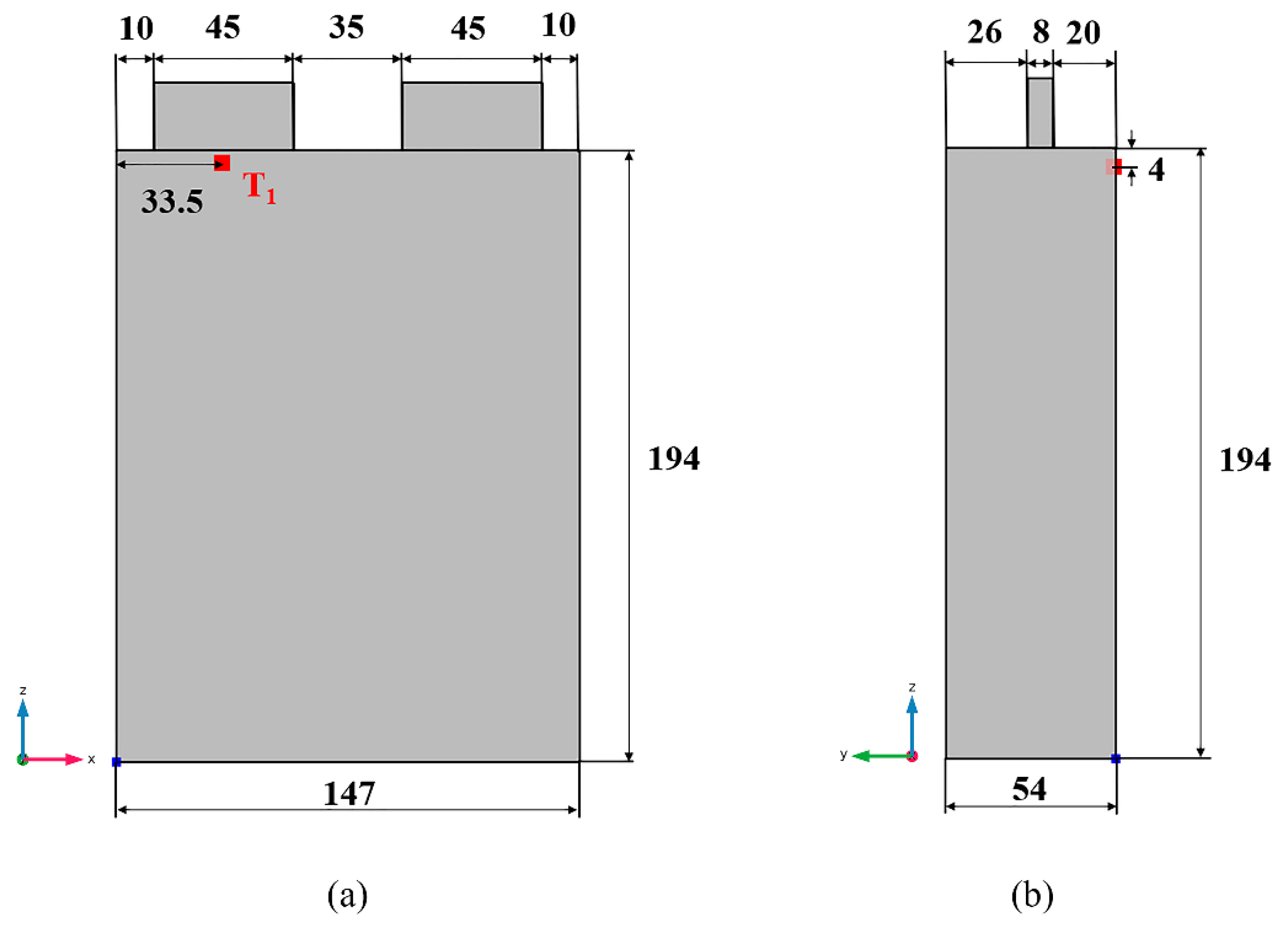
According to the parameters used by Kim et al. [47,48] in the study of the thermal behavior of prismatic battery cells under various ambient air temperatures, this paper conducts transient modeling of prismatic battery cells with LiMn₂O₄ as the cathode material, maintaining the same geometric structure, parameter configuration, and boundary condition settings. In Figure 4, the overall initial temperature of the prismatic battery is set to the ambient temperature of 25 °C. The surface heat transfer coefficient of the surface in contact with the air is set to 10 W/(m²‧K), and the surface emissivity of the surface radiation to the environment is set to 0.8. The detailed parameters of the prismatic battery are shown in

Table 2. Detailed parameters of the prismatic battery for experimental verification.

Parameter	Thermal Conductivity (W/(m‧K))	Heat Capacity at Constant Pressure (J/(kg‧K))	Density (kg/m3)	Reference
Positive Current Collector	238	900	2700	[49]
Negative Current Collector	400	385	8960

. Under the condition that the ambient air temperature is set to 25 °C, the voltages and battery capacities at point T₁ near the positive electrode, as shown in Figure 4 under 1C, 3C, and 5C discharges, are calculated and then compared with the experimental results obtained by Kim et al. [48] to verify the accuracy of the simulation.

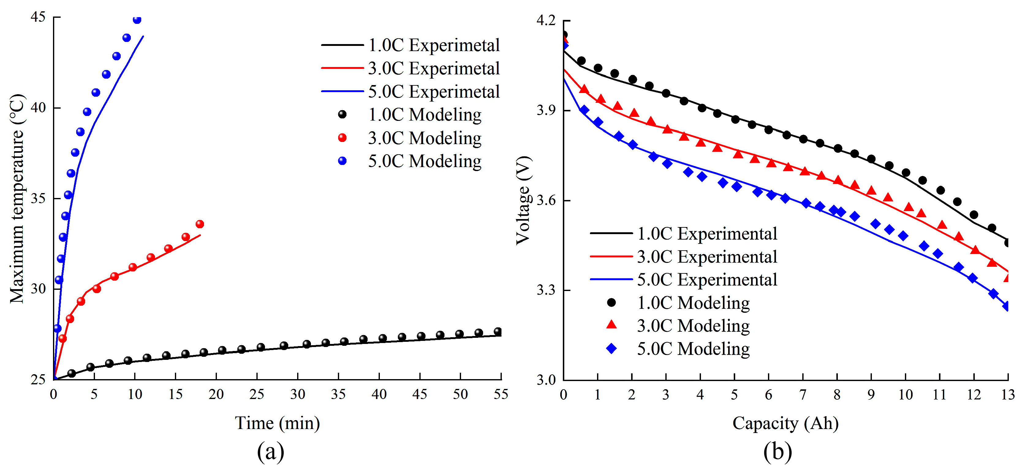
Figure 5 compares simulation and experimental results for voltage–capacity curves and maximum temperature of LIBs under different constant current discharge rates with the experimental results for the simulation model. Figure 5b shows the maximum model experiment errors of 2.06%, 2.57%, and 2.73% under 1C, 3C, and 5C discharge. Error increases slightly with higher rates but remains low overall. Figure 5a shows higher accuracy, with maximum errors of 0.01%, 0.02%, and 0.28% under 1C, 3C, and 5C discharge, confirming the theoretical reliability and engineering applicability of the Multiphysics-built lithium-ion battery cell transient model.

2.8. SVAR Model

The time-varying curves of various parameter variables were obtained through simulation. The electrochemical and thermal relationships of LIBs are extremely complex. Analyzing only the electrochemical and thermal laws of a single variable makes it difficult to meet the research requirements. Common time-series models include autoregressive integrated moving average (ARIMA), SVAR, and long short-term memory (LSTM) networks. The ARIMA model, based on linear regression, decomposes time series into autoregression, moving average, and differencing components. It captures univariate dynamics and lag dependencies but cannot incorporate other variables or describe their dynamic responses. The SVAR model, an extension of ARIMA, is a structured statistical model. It identifies structural shocks (causal relationships) between variables via matrix decomposition, suitable for multivariate economic or specific systems requiring causal analysis. The LSTM model is a data-driven nonlinear mapping, adaptively capturing nonlinear patterns and long-term dependencies. However, it involves complex calculations, requires extensive training and parameter tuning, and cannot explain the causes of inter-factor relationships.

This paper employs a Bayesian-estimated SVAR model based on the vector autoregression (VAR) framework to study dynamic response relationships among any four thermal and electrochemical variables. The lag coefficient matrix A_l is identified using Markov chain Monte Carlo (MCMC) to generate posterior samples, with short-term constraints applied recursively according to variable order to enhance model realism.

A simplified form of VAR is shown in Equation (40):

$$Y_t=\beta +\sum _{l=1}^3{B}_l{Y}_{t-1}+u_t,u_t~N(0,\mathsf{\Sigma })$$

(40)

where Y_t is the dependent variable vector at time t; β, B, and u_t are the conforming vectors and matrix of coefficients and residuals, respectively.

A SVAR model with 3 lags is applied, as shown in Equation (41):

$$A_0{Y}_t=d+\sum _{l=1}^3{A}_l{Y}_{t-1}+e_t$$

(41)

where A₀ is the parameter matrix for the current period, including coefficients of simultaneous relationships between endogenous variables; d is the conforming vector of coefficients; A_l is the lag coefficient matrix; e_t is the structural shock vector, as shown in Equation (42).

$$e_t=A_0^{-1}{u}_t$$

(42)

The SVAR model, a time-series method widely used in economics to analyze relationships among multiple variables, is applicable to studying electrochemical and thermal variables of LIBs. Methodologically, SVAR’s structured shock decomposition and dynamic time-series modeling mirror the multi-factor coupling in battery parameter analysis. Both emphasize causal transmission and lag effects of system variables, using impulse response functions (IRF) to quantify time-varying impacts—such as oil price shocks on financial risks or operational changes on battery temperature. In adaptability, the time-varying degradation of battery parameters across life cycles aligns with periodic evolutions of economic macro-indicators. SVAR’s capability to capture time-varying parameters accurately describes the nonlinear dynamics of battery temperature rise. In universality, the model constructs causal networks via simultaneous correlation matrices and quantifies factor contributions through error decomposition. Applicable to both electrochemical parameter evaluation and battery temperature warning, it bridges economic systemic risk analysis with engineering science, offering a universal quantitative framework for time-series analysis of cross-disciplinary complex systems. Model results reflect dynamic variable relationships. Impulse response functions reveal how other variables respond over time to external shocks. Variance decomposition shows the contribution of each variable to fluctuations in others, clarifying their relative importance in the system.

2.9. Integrated Learning Regression Prediction System

While the SVAR model enables in-depth analysis of variable relationships, the data it requires rely on traditional calculation methods such as experiments and simulations, which are often time-consuming and difficult to meet the needs of rapid research and optimization, resulting in high time costs. To reduce the cost, this paper proposes a multi-output regression prediction system based on ensemble learning—the ensemble learning regression prediction system. This system integrates multiple advanced machine learning models to accurately predict key parameters such as the maximum temperature difference (MTD), average temperature, and uniformity index of the battery, improving the research efficiency. The system architecture of the ensemble learning regression prediction system is shown in Figure 6. Its core advantage lies in the ability to comprehensively utilize three advanced machine learning techniques, namely, random forest, gradient boosting, and extra trees, to enhance the accuracy of prediction. Its system architecture is shown in Figure 6. Figure 6a represents the data preparation stage, where the original data are preprocessed to improve their quality and adapt them for training. Figure 6c shows the construction of basic models, such as random forest, gradient boosting, and extra trees, and the creation of ensemble models in the form of multi-output regressors for each basic model. The preprocessed data and ensemble models are input into the training and evaluation process to construct the ensemble model, as shown in Figure 6d. The data are split to obtain the X-test set (X-test) and Y-test set (Y-test), which are combined with the trained ensemble prediction model (ensemble-pred) and the updated scaler, and work together with the ensemble models to evaluate the prediction results, completing the system construction. As shown in Figure 6e, when using this system for extrapolation prediction, first the scaler is called to standardize and update the input data, and then, the ensemble-pred performs the calculation to complete the extrapolation prediction process.

Key hyperparameters of the base models are systematically tuned, including tree count, maximum depth, and minimum samples per split, using random search with cross-validation. Each hyperparameter combination is evaluated on the validation set using metrics such as R- square, root-mean-square error (RMSE), mean absolute error (MAE), etc., documenting results in detail. The optimal hyperparameter combination is selected based on comprehensive validation set performance across multiple metrics to balance high predictive accuracy with strong generalization. The random forest employs 500 decision trees, requiring 3 minimum samples for node splitting, with a max depth limited to 15 to avoid overfitting. In the gradient boosting model, the number of decision trees is set to 300, the maximum depth of each tree is 8, and the learning rate is set to 0.1. The extremely randomized trees model has 400 trees with a maximum depth 12. This paper constructs the framework of the integrated learning regression prediction system based on the Python 3.9 programming environment. During the training process, the training set and the test set are divided in a ratio of 8:2. Twelve working conditions (0.3C–1.5C charge/discharge) yield 151 time-series samples each, totaling 1812 data points. The training data file requires at least 6 columns of data, where the first three columns are input features and the last three columns are target variables. The three columns of input features are current rate, charging/discharging mode (charging is digitized as 1, discharging is digitized as 2), and representative numbers of the time series (a sequence of numbers increasing at fixed intervals). The three columns of target variables are MTD, mean temperature, and UI, and all target variables are derived from the calculation results of the battery simulation model. In the integrated system’s input features, current rate and charge/discharge mode act as independent variables for the battery simulation model, with time-interval incremental numerical sequences ensuring smooth operation. The system uses standardization for normalization to eliminate rate-related numerical differences affecting machine learning model training. Outliers are processed via standard deviation; feature interactions and squared/cubic terms are added to capture nonlinear relationships and high-order effects, improving model performance. To evaluate the accuracy of the integrated learning regression prediction system, this paper uses multiple evaluation indicators such as R-square, RMSE, MAE, mean absolute percentage error (MAPE), and correlation coefficient (r). The calculation formulas of the evaluation indicators are shown in Equations (43)–(47) [50,51].

$$R^2=1-{\sum }_{i=1}^N {\displaystyle \frac{{\left(Y_{p,i}-Y_{a,i}\right)}^2}{Y_{a,i}^2}},$$

(43)

$$\mathrm{R}\mathrm{M}\mathrm{S}\mathrm{E}=\sqrt{{\displaystyle \frac{1}{N}}\sum _{\mathrm{i}=1}^N {\left(Y_{p,i}-Y_{a,i}\right)}^2}$$

(44)

$$\mathrm{M}\mathrm{A}\mathrm{E}={\displaystyle \frac{1}{N}}\sum _{\mathrm{i}=1}^N |Y_{p,i}-Y_{a,i}|$$

(45)

$$\mathrm{M}\mathrm{A}\mathrm{P}\mathrm{E}={\displaystyle \frac{100\mathrm{\%}}{N}}\sum _{\mathrm{i}=1}^N \left|{\displaystyle \frac{Y_{p,i}-Y_{a,i}}{Y_{a,i}}}\right|$$

(46)

$$r={\displaystyle \frac{\sum _{i-1}^N (X_{p,i}-\overline{X})(Y_{p,i}-\overline{Y})}{\sqrt{\sum _{i=1}^N (X_{p,i}-\overline{X}{)}^2}\sqrt{\sum _{i=1}^n (Y_{p,i}-\overline{Y}{)}^2}}}$$

(47)

where X_p,i is the model-predicted value of variable X; Y_p,i is the model-predicted value of variable Y; Y_a,i is the actual value; N is the number of samples; $\overline{X}$ is the average value of variable X; $\overline{Y}$ is the average value of variable Y.

3. Results

3.1. Effect of Charge and Discharge Rate on Battery Temperature

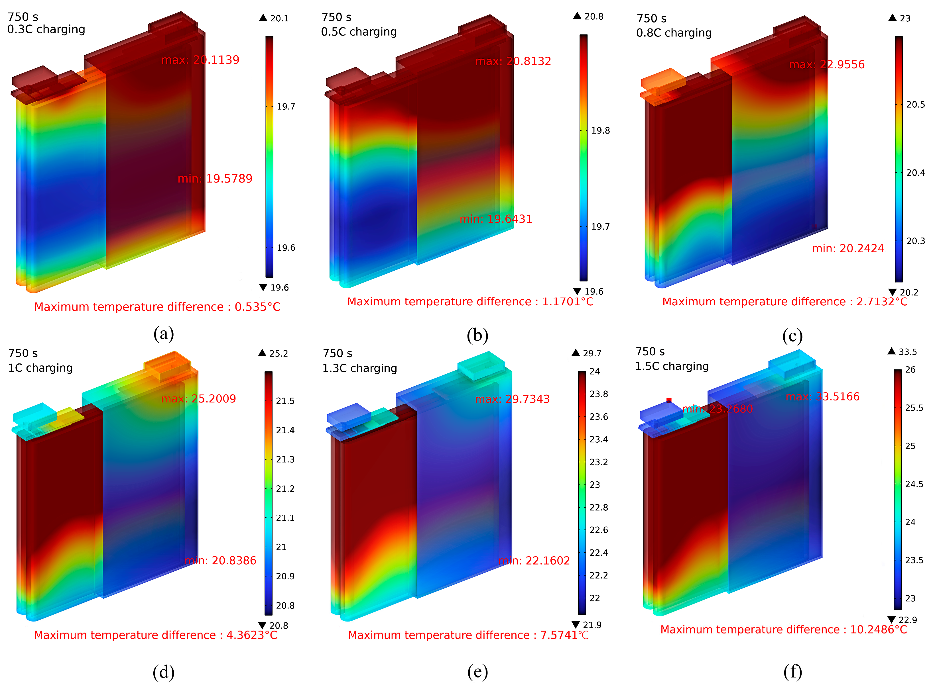
Figure 7 shows the overall temperature distribution of the battery at different charging rates. It indicates that during lithium-ion battery charging, the maximum temperature is concentrated at the positive tab, while the minimum is at a position far from it. With the negative grounded and the positive as the charging port, the positive tab first receives different rate currents. As the charging rate is a key factor for battery electrothermal characteristics (confirmed by Guo et al. [52] to determine electrode current), the maximum temperature is always at the positive tab. At the start of charging, the battery surface and positive/negative electrodes have uniform temperatures close to the ambient temperature, in line with Mei et al. [36]. During charging, as the rate increases, the maximum temperature of the lithium-ion battery rises 1.03–1.67 times, with the minimum of 1–1.19 times and the MTD of 2.19–19.16 times. The MTD is the most affected, followed by the maximum temperature, and the minimum temperature is the least affected. At high charging rates (1.3C and 1.5C), the MTD of the battery reaches 7.5741 °C and 10.2486 °C, respectively, exceeding 5 °C, which may cause danger and requires prompt cooling.

The overall temperature distribution of the battery at different discharge rates is presented in Figure 8. Results in Figure 8 show that with the increase in discharge rate, the maximum temperature rises 1.04–1.67 times, with the minimum of 1–1.19 times and the MTD of 2.19–19.16 times. Comparing temperature data at the same current rate reveals that the maximum and minimum temperatures and MTD during battery discharge are nearly the same as in charging, indicating little impact of the charge/discharge cycle on the electrothermal properties of lithium-ion batteries. During battery discharge, higher rates initiate high-speed electrochemical reactions, causing uneven utilization of active materials at electrodes and excessive heat accumulation, with electrode temperatures much higher than other areas [21]. At high-rate discharge, the rapid movement of lithium ions creates a high concentration difference, increasing the radial stress gradient of active particles at electrodes [21]. This may lead to particle failure and increased internal resistance and may affect normal charge/discharge processes.

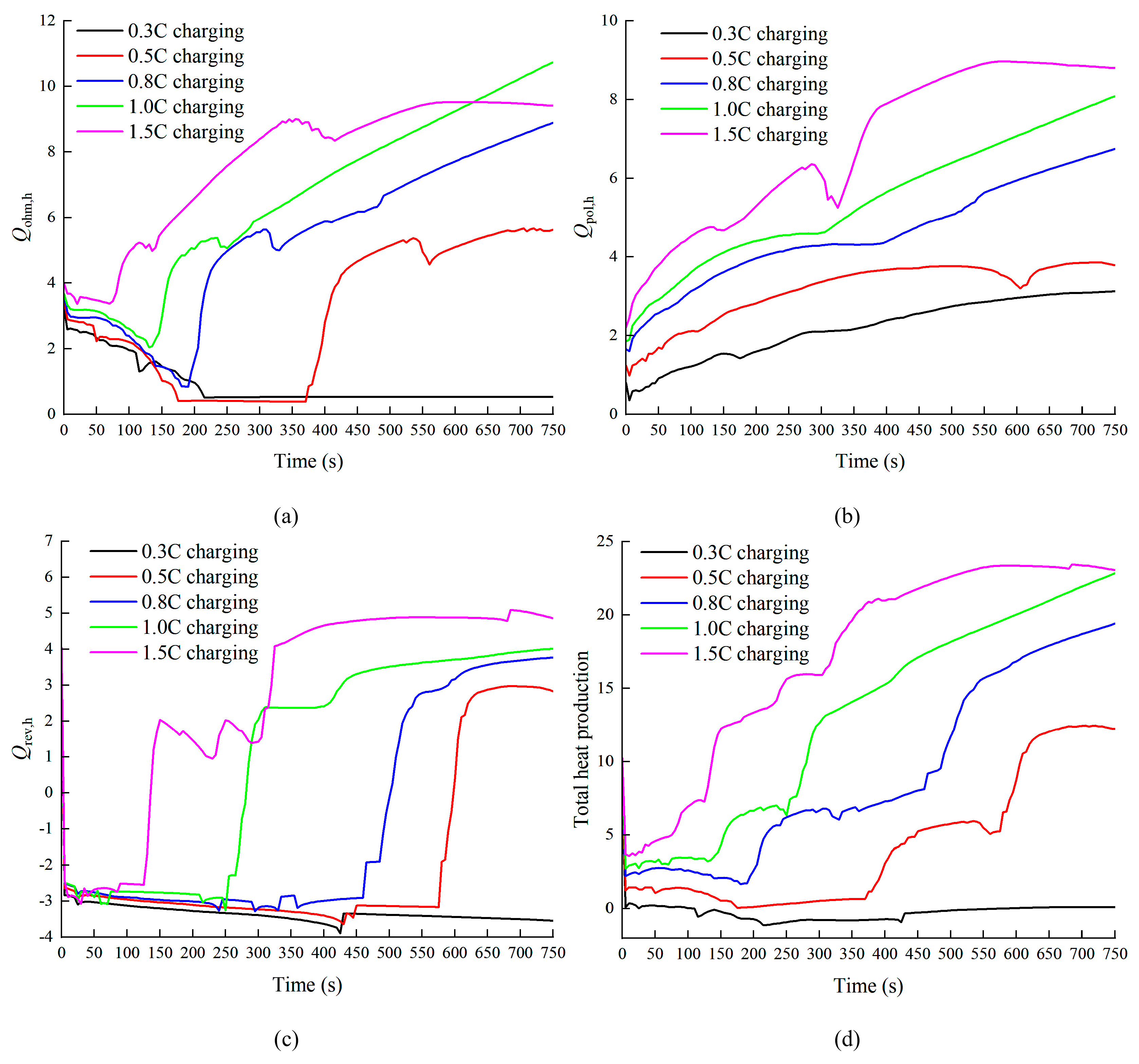
Figure 9 shows the variations of ohmic, polarization, reversible, and overall heat generation of the battery over time at different charging rates. The calculation point is selected at the junction of the positive and negative electrodes and current collectors in the battery stack near the negative electrode of the two-dimensional planar battery. As the charging rate increases, the rates of the three types of heat generation increase significantly. Reversible heat generation has the fastest growth rate, followed by polarization heat generation, and ohmic heat generation is the slowest. Reversible heat comes from the chemical reactions at the positive and negative electrodes. As the charging rate speeds up, as shown in Figure 7, the battery temperature rises. Within a certain safe temperature range, the temperature rise promotes chemical reactions and accelerates the generation of reversible heat. The higher the rate, the earlier this acceleration point occurs. Over time, the polarization and ohmic heat generation under the 1.5C charging condition are lower than those under the 1C condition. Since polarization and ohmic heat generation are related to over-potential, the temperature rise in the constant-current stage accelerates chemical transport and reduces the ion concentration on the electrode surface, thus reducing the over-potential [11]. This improves the internal reaction and ion migration rates, and the heat generation tends to be stable.

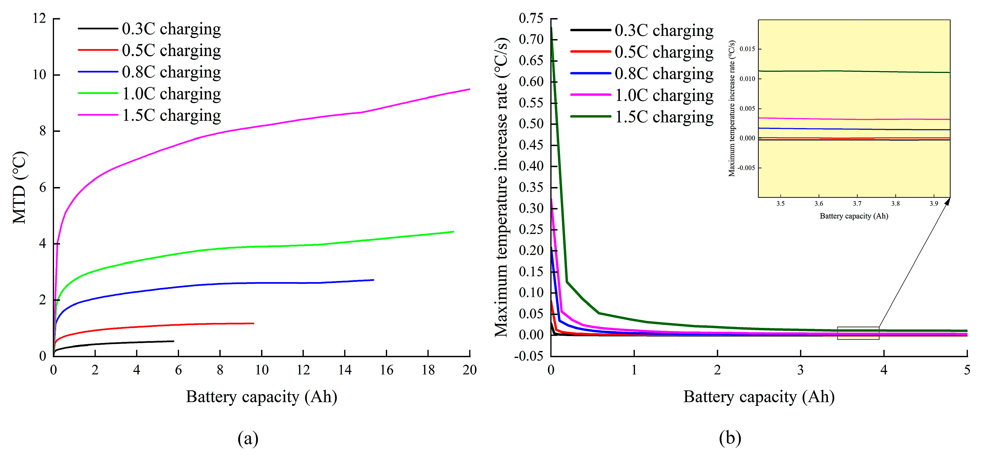
The MTD of LIBs reflects the temperature uniformity inside the battery and among individual cells, which is an important thermodynamic indicator. The battery capacity reflects the aging and health status of the battery, serving as a crucial electrochemical indicator. To explore the relationship between the battery heat and electrochemical parameters, the curves of the MTD and the maximum temperature growth rate versus the battery capacity are plotted, as shown in Figure 10. At the initial stage of charging, the MTD of the battery under different charging rates increases rapidly, leading to a significant unevenness of the battery temperature in the short term, as shown in Figure 7 (the same applies during discharging, as shown in Figure 8). As time goes by, the growth rate of the maximum battery temperature decreases and tends to stabilize, causing the MTD of the battery to level off in the later stage and eventually stabilize near 0.00. This further confirms the changes of the three heat sources with the charging rate in Figure 9.

3.2. Dynamic Impact Analysis Results of the Structured Vector Autoregression Model

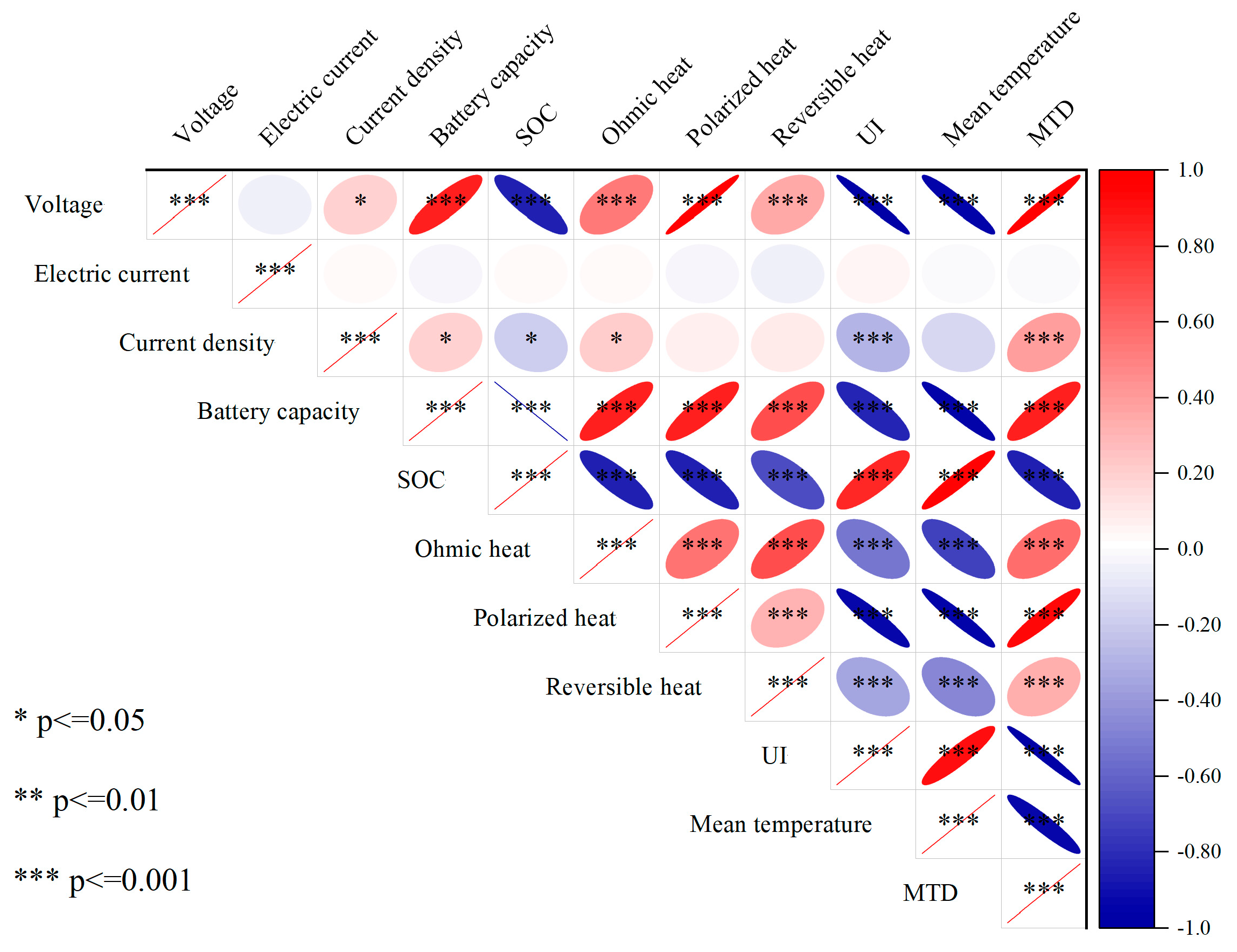
The relationship between the electrochemistry and the heat of LIBs is complex. To explore the interaction between electrochemical and thermal variables, a correlation heatmap of the two during 0.5C charging is plotted, as shown in Figure 11. Figure 11 shows that voltage, current density, battery capacity, and MTD are significantly positively correlated when the p-value is less than 0.001, and the SOC of the battery and the MTD are significantly negatively correlated when the p-value is less than 0.001. The correlation coefficients between voltage, UI, average temperature, and MTD are −0.9731, −0.9486, and 0.9725, respectively, indicating a strong correlation. Based on this, this paper takes the interaction relationships between UI, average temperature, MTD, and voltage as the starting point to explore the mutual influence mechanism of the electrochemical and thermal characteristics of LIBs during 0.5C charging.

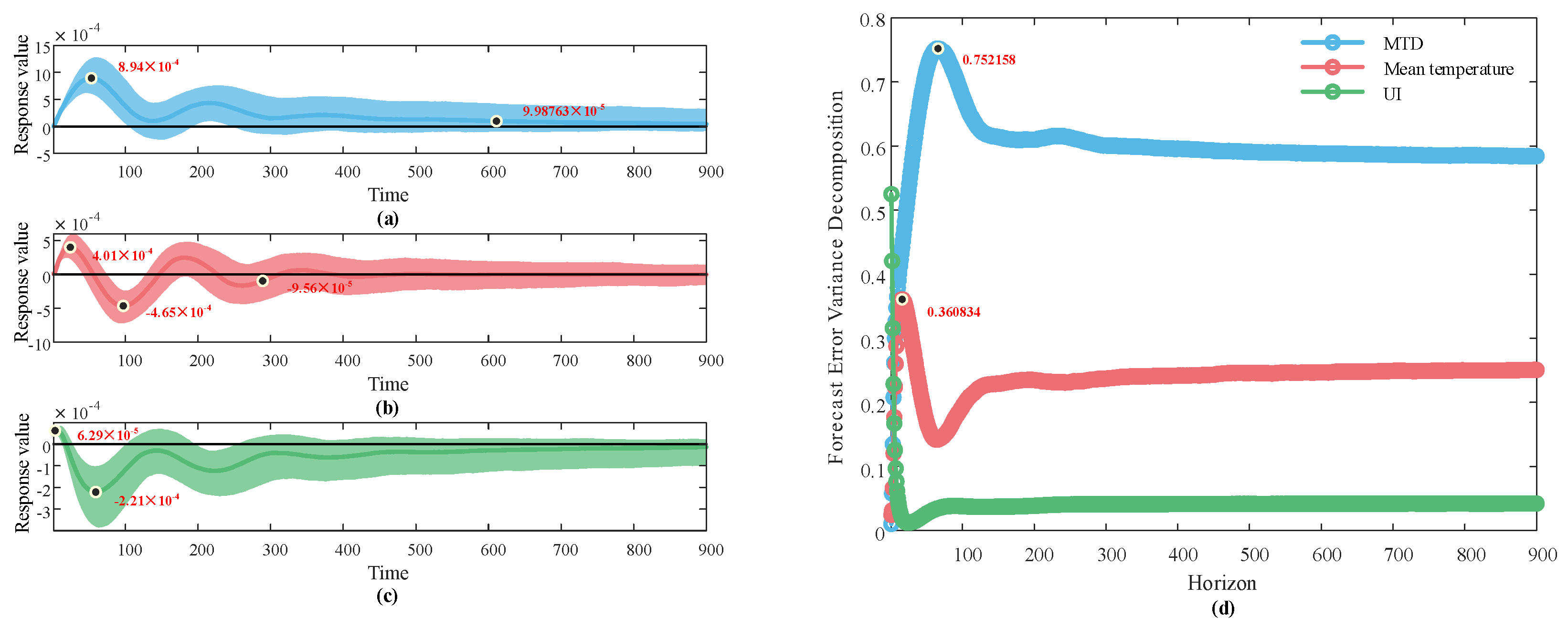
Figure 12 illustrates the synergistic effects of the MTD, average temperature, and UI on the voltage during 0.5C charging. The solid line in the frequency band represents the median of the thermal characteristic effects, with the upper and lower boundaries being the 16th and 84th percentiles, respectively [53]. The IRF cycle value is set to 900. In Figure 12a, the MTD is positively correlated with the voltage, in line with Figure 11. Its impact on voltage peaked at 8.94 × 10⁻⁴ during the 53rd IRF cycle, with a rapid response. This was due to the instantaneous heat generation from the battery’s ohmic resistance at the initial charging stage, which caused a rapid rise in local battery temperature and a sharp increase in the MTD. At cycle 611, heat began to diffuse within the battery via thermal conduction, causing the MTD to gradually decrease and then stabilize regionally. The impact is below 1.00 × 10⁻⁴, having a long duration and great influence. The overall impact decays with the cycle, and the voltage eventually returns to stability or reaches a new equilibrium. In Figure 12b, the average temperature and the voltage alternate between positive and negative correlations initially, and finally show a negative correlation, with complex interactions, as well as indirect and lagging effects. During the 24th IRF cycle, voltage shock superimposed ohmic and polarization heating, causing a rapid average temperature rise and a positive correlation peak of 4.01 × 10⁻⁴. Between IRF cycles 20 to 97, undissipated heat caused a continued temperature rise, showing a negative correlation between average temperature and voltage. At cycle 97, thermal conduction-heat generation equilibrium stabilized the impact, with a rapid negative correlation peak of −4.65 × 10⁻⁴. Its impact on voltage exhibited a positive correlation peak of 4.01 × 10⁻⁴ at the 24th IRF cycle and a negative correlation peak of −4.65 × 10⁻⁴ at the 97th cycle, with rapid responses. At cycle 289, the impact was below 1.00 × 10⁻⁴, with a short duration and little influence, probably due to changes in internal reactions and ion migration in the battery at high temperatures [11]. Figure 12c shows that the complexity of the impact of UI on the voltage is lower than that of the average temperature. In the short term, UI increases the voltage, while in the long term, the opposite is true. Its impact on the voltage has a positive correlation peak of 6.29 × 10⁻⁵ at IRF cycle 3 and a negative correlation peak of −2.21 × 10⁻⁴ at cycle 59, with a quick response. The overall impact was almost all below 1.00 × 10⁻⁴, with little influence. Figure 12d reveals that under 0.5C charging, in the short term, the MTD has the most significant impact on the voltage, followed by the average temperature, with UI having the weakest impact. As the IRF cycle progresses, the impacts of the MTD and the average temperature on the voltage first increase and then decrease, and then increase briefly before stabilizing. The MTD reaches a maximum contribution value of 75.22% at IRF cycle 66 and then stabilizes around 59.00%. The average temperature reaches a maximum contribution value of 36.08% at IRF cycle 16 and then stabilizes around 23.00%. The impact of UI on the voltage first decreases and then increases, tending to be gentle in the long term, and the final contribution value stabilizes around 4.00%. The MTD has the greatest influence on the voltage, followed by the average temperature, and UI has the weakest influence. Moreover, changes in the MTD and the average temperature tend to increase the risk of voltage changes, which is significant in most periods.

Figure 13 is a correlation heatmap of electrochemical characteristics and thermal characteristics during 1C discharging. Compared with Figure 11, the correlation between voltage and thermal characteristic variables is significantly enhanced at a higher current rate, and it is significantly positively correlated, except for UI. This indirectly shows that an increase in voltage is not conducive to the uniformity of the battery temperature. Consistent with Figure 11, the correlation between current and thermal characteristic variables is still not significant. As can be seen from Figure 13, voltage and current density have a significant positive correlation with the MTD. The correlation coefficients between voltage, current density, and the MTD are 0.9730 and 0.5054, respectively. To explore the synergistic effects among voltage, current density, and the MTD, UI is introduced to assist in the calculation of SVAR.

Figure 14 shows the interaction between the battery’s electrochemical and thermal characteristics during 1C discharging, with IRF’s period set at 300. Figure 14a reveals the complex impact of voltage increase on the MTD under high-rate discharging. It shows alternating positive and negative correlations, finally reaching a new equilibrium. At IRF cycle 97, the voltage’s impact on the MTD peaks at 5.84 × 10⁻⁴, 2.82 times the negative peak of −2.07 × 10⁻⁴, indicating a rapid and significant response of the MTD to voltage changes. At IRF cycle 164, a one-unit voltage increase has less than 1.00 × 10⁻⁴ impact on the risk of MTD increase, showing a short-lasting and weak impact of voltage on it. Figure 14b shows similar trends of current density and voltage impacts on the MTD under high-rate discharging. Current density reaches a negative peak of −1.46 × 10⁻³ at IRF cycle 47 and a positive peak of 6.29 × 10⁻⁴ at IRF cycle 134, more significant than the voltage’s impact. At IRF cycle 206, a one-unit current density increase has less than 1.00 × 10⁻⁴ impact on the risk of MTD increase, with a longer-lasting response than voltage. However, both voltage and current density responses to the MTD impact will return to a stable state or a new equilibrium as the IRF cycle goes on. Figure 14d shows the influence degrees of voltage, current density, and UI on the MTD during 1C discharging. Initially, their contribution values decrease. Current density reaches 4.62% at IRF cycle 21 and then stabilizes around 23%. Voltage’s contribution is 6.94% at the start and stabilizes around 5%. Overall, current density has a greater impact on the MTD than voltage. Although their impacts alternate between positive and negative, both voltage and current density tend to increase the MTD risk, consistent with the positive correlation in Figure 13.

3.3. Prediction Results of the Integrated Learning Regression Prediction System

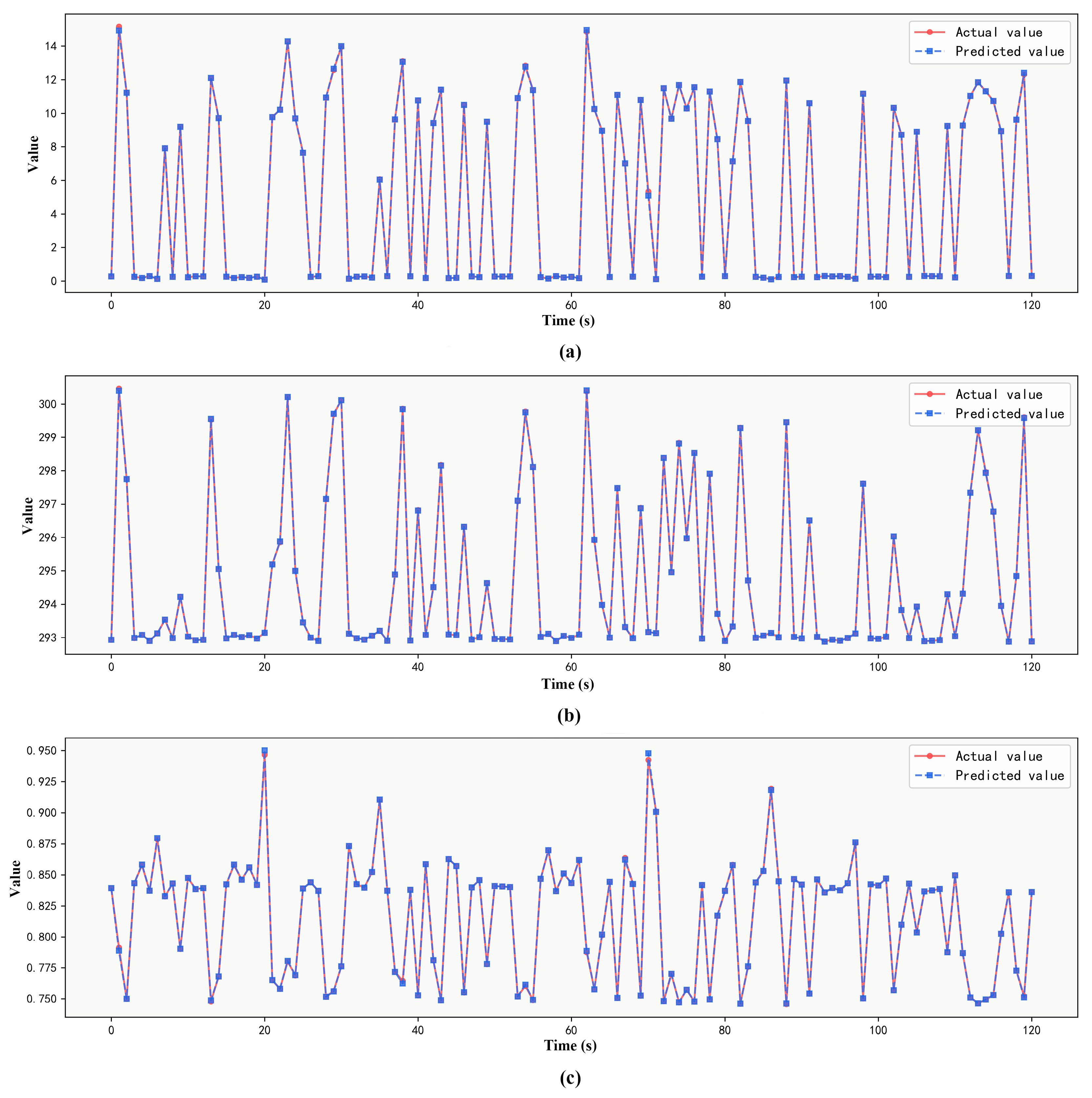
Figure 15 shows the precision radar chart of the prediction model. Figure 15a–c correspond to the system’s self-prediction precision results for Output 1, Output 2, and Output 3, respectively. The results in Figure 15a show that for Output 1 prediction, the overall model’s R-square is 0.9998, which is higher than the random forest’s 0.9996 and slightly lower than those of the gradient boosting tree and extremely randomized trees (both 0.9999). However, its RMSE, MAE, and MAPE are better, indicating a stronger prediction ability for Output 1. Figure 15b shows that among the three basic models and the overall model, the maximum R-square is 1 for the extremely randomized trees. The overall model’s MASE is 0.0083, lower than the gradient boosting tree’s 0.0184 and the extremely randomized trees’ 0.0115, and its MAE is 0.0029, close to the extremely randomized trees’ 0.0016. The overall model predicts Output 2 better. In Figure 15c, the overall model’s R-square is 0.9983, higher than the random forest’s 0.9973 and the gradient boosting tree’s 0.9943. RMSE is 0.0019 lower than the gradient boosting tree’s 0.0035, and r is 0.9992 higher than both, showing a better prediction for Output 3. Both the three basic models and the integrated model have high prediction accuracy. Moreover, considering algorithm complexity and program operation, the prediction system’s trend prediction R-square reaches 0.7769, indicating a relatively high accuracy in analyzing the trends of the three output values of LIBs at different charging and discharging rates. In conclusion, the integrated learning regression prediction system developed in this paper has extremely high prediction accuracy, is suitable for predicting the dependent variable values of LIBs at different charging and discharging rates, and can be used for subsequent research.

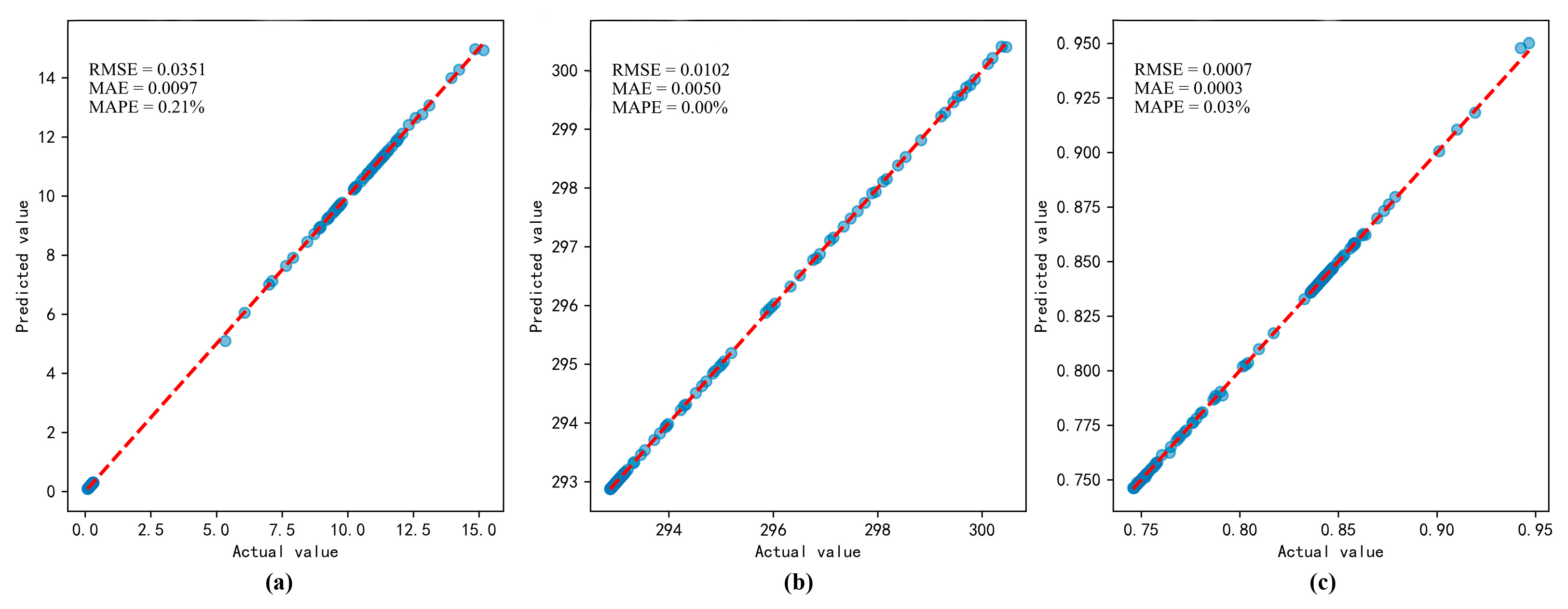
To evaluate the generalization and extrapolation capabilities of the integrated learning regression prediction system, this paper adds the analysis of four working conditions: 0.2C charging and discharging and 1.6C charging and discharging, and uses the system model to predict the data. The comparison between the predicted and actual values is shown in Figure 16. Figure 16 shows that the data points of the three outputs are all close to the red dotted line, indicating that the predicted values are very close to the actual values. Among the three outputs, Output 3 exhibits the smallest RMSE (0.0007) and MAE (0.0003), with a very low MAPE of 0.03%, indicating the system’s strongest performance in UI prediction. Output 1 and Output 2 have slight deviations at some extreme values but perform well overall.

Figure 17 is the prediction accuracy chart of the integrated learning regression prediction system. Taking Output 1 (MTD) as an example, the R-square value of the model in predicting the MTD is 0.9996, the RMSE is 0.3448, the MAE is 0.0732, the MAPE is 0.0056, and r is 0.9998, indicating that the prediction system model has a good prediction ability for the data of these four operating conditions. Combining with the comparison between the prediction results of the three outputs and the true values in Figure 15, it can be concluded that the integrated learning regression prediction system has extremely high prediction accuracy. Furthermore, when extrapolating predictions for four working conditions (0.2C and 1.6C charge/discharge) based on 1812 existing samples, the system completes calculations within 30 s—significantly faster than the cumulative 58,881 s required for simulations. This highlights the system’s remarkable efficiency in reducing time costs.

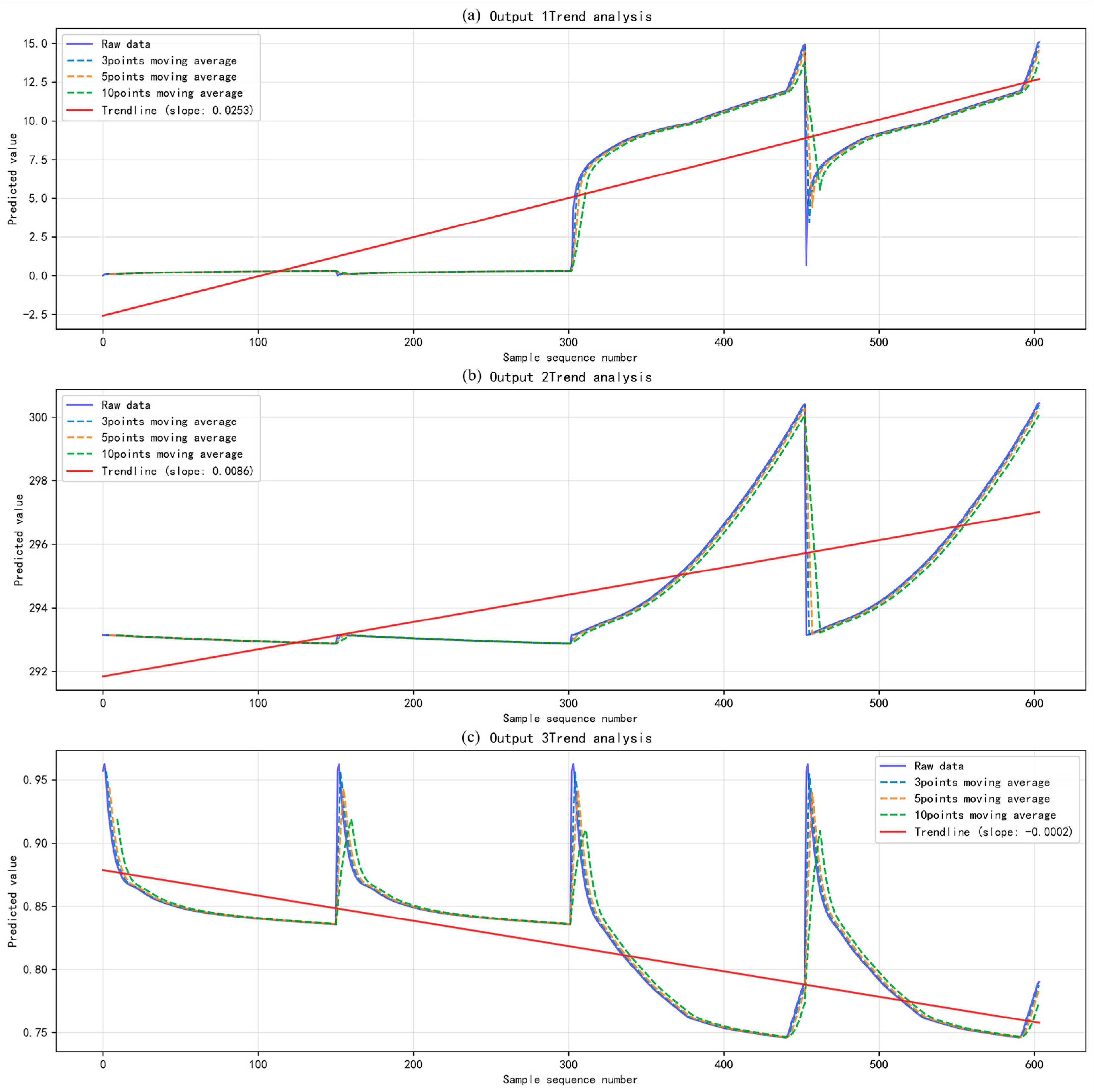
The integrated learning regression prediction system developed in this paper can not only accurately predict the MTD, average temperature, and UI under specific current rates and charging and discharging modes, but it can also fit the trend lines of the input current rates and charging and discharging modes and conduct periodic tests. For the MTD, average temperature, and UI, the prediction results of the trend indicators of the system for the four operating conditions are shown in

Table 3. Trend indicators.

	MTD	Mean Temperature	UI
Mean Value	5.0574 K	294.4292 K	0.8183
Standard Deviation	5.0272	2.0964	0.0482
Coefficient of Variation	0.9940	0.0071	0.0589
Maximum Value	15.0845 K	300.4394 K	0.9627
Minimum Value	0.0103 K	292.8757 K	0.7459
Range	15.0742 K	7.5638 K	0.2167
Trend Slope	0.0253 K/s	0.0086 K/s	−0.0002
Trend R-square	0.7726	0.5094	0.5263
Autocorrelation Coefficient	0.9922	0.9899	0.9773

. Table 3 shows that although the R-square of the trend fitting is low, the autocorrelation coefficient is close to 1, indicating that the model has a high internal correlation. Considering the complexity of the algorithm and the implementation of the program comprehensively, in the presence of certain errors, the integrated learning regression prediction system shows good performance in predicting the trends of the four operating conditions: 0.2C charging, 0.2C discharging, 1.6C charging, and 1.6C discharging.

Figure 18 shows the predictive trend analysis of the system under four operating conditions: 0.2C charging, 0.2C discharging, 1.6C charging, and 1.6C discharging. Figure 18 shows that the 3-point moving average nearly coincides with the original data line, indicating stable short-term data and accurate short-term trend capture during extrapolation. The 5-point moving average generally follows the original data line, overlapping at first, with a slight deviation at the end, and being smoother, showing that the system filters short-term fluctuations and presents a stable medium-term trend. The 10-point moving average has a similar trend to the original data line throughout, reflecting the system’s strong ability to grasp long-term trends. Overall, the integrated learning regression prediction system in this paper has strong abilities in grasping both short-term and long-term trends when predicting the trends of extrapolated conditions.

4. Discussion

This paper deeply explores the electrochemical–thermal coupling characteristics of 150Ah prismatic lithium iron phosphate batteries, yielding remarkable results. However, there are still some deficiencies in this paper’s research. Model assumptions were simplified, neglecting electrode volume change, side reactions, current collector heating, battery aging effects on heat generation/temperature distribution, safety failures (e.g., internal short circuits), and simplified electrolyte diffusion. These limit accuracy, generalizability, and prediction precision in long-term cycling, extreme conditions, and safety warning scenarios. Additionally, the economics-derived SVAR model may fail to capture nonlinear/time-varying relationships in complex battery electrothermal coupling. Constrained by training conditions and battery systems, the ensemble learning system’s generalizability needs improvement. Future work will optimize the system by refining assumptions, incorporating practical factors, enhancing parameter validation, enriching verification conditions, and integrating algorithms to advance lithium-ion battery research.

5. Conclusions

This paper develops a 3D electrochemical–thermal coupling model for 150 Ah lithium iron phosphate batteries. Using SVAR to explore multi-variable synergy, it proposes an integrated learning regression prediction system that combines multiple models to precisely predict key battery parameters. Conclusions are as follows:

(1) The charge/discharge rate significantly affects thermal characteristics. During charging, increasing the rate from 0.3C to 1.5C raises the maximum battery temperature up to 1.67 times and the maximum temperature difference up to 19.16 times; at 1.3C and 1.5C, the maximum temperature differences reach 7.57 °C and 10.25 °C, respectively, both exceeding the 5 °C safety threshold. The heat generation rate increases significantly with the rate, with reversible heat increasing the fastest, followed by polarization heat and then ohmic heat. Discharge temperature characteristics are similar to those during charging.

(2) Electrochemical and thermal parameters interact dynamically. During 0.5C charging, voltage is strongly positively correlated with the maximum temperature difference, with a correlation coefficient of 0.9725 and p < 0.001, and strongly negatively correlated with the temperature uniformity index, with a correlation coefficient of −0.9731 and p < 0.001; SOC is significantly negatively correlated with the maximum temperature difference. The SVAR model shows that during 1C discharge, the peak impulse response of voltage to the maximum temperature difference is 5.84 × 10⁻⁴ at the 97th cycle; the peak impulse response of current density to the maximum temperature difference is −1.46 × 10⁻³ at the 47th cycle, and the influence of current density lasts longer, approximately 206 cycles.

(3) The developed integrated learning regression prediction system performs well for lithium-ion batteries at different charge/discharge rates. Basic and integrated models have high accuracy. In the generalization evaluation, predicted values are close to the true ones. Trend analysis shows the system can well grasp short-, medium-, and long-term trends. It is suitable for lithium-ion battery dependent-variable prediction and further research.

References

1. Lei, D.; Wang, Y.; Fu, J.; Zhu, X.; Shi, J.; Wang, Y. Electrochemical-thermal analysis of large-sized lithium-ion batteries: Influence of cell thickness and cooling strategy in charging. Energy 2024, 307, 132629. [Google Scholar] [CrossRef]
2. Zhao, R.; Gu, J.; Liu, J. An investigation on the significance of reversible heat to the thermal behavior of lithium ion battery through simulations. J. Power Sources 2014, 266, 422–432. [Google Scholar] [CrossRef]
3. Xiong, R.; Zhang, K.; Qu, S.; Tian, J.; Shen, W. A fast pre-heating method for lithium-ion batteries by wireless energy transfer at low temperatures. eTransportation 2023, 16, 100227. [Google Scholar] [CrossRef]
4. Ianniciello, L.; Biwolé, P.H.; Achard, P. Electric vehicles batteries thermal management systems employing phase change materials. J. Power Sources 2018, 378, 383–403. [Google Scholar] [CrossRef]
5. An, Z.; Jia, L.; Wei, L.; Dang, C.; Peng, Q. Investigation on lithium-ion battery electrochemical and thermal characteristic based on electrochemical-thermal coupled model. Appl. Therm. Eng. 2018, 137, 792–807. [Google Scholar] [CrossRef]
6. Liu, T.; Ge, S.; Yang, X.-G.; Wang, C.-Y. Effect of thermal environments on fast charging Li-ion batteries. J. Power Sources 2021, 511, 230466. [Google Scholar] [CrossRef]
7. Zhang, X.; Chang, X.; Shen, Y.; Xiang, Y. Electrochemical-electrical-thermal modeling of a pouch-type lithium ion battery: An application to optimize temperature distribution. J. Energy Storage 2017, 11, 249–257. [Google Scholar] [CrossRef]
8. Liu, Y.; Tang, S.; Li, L.; Liu, F.; Jiang, L.; Jia, M.; Ai, Y.; Yao, C.; Gu, H. Simulation and parameter identification based on electrochemical- thermal coupling model of power lithium ion-battery. J. Alloys Compd. 2020, 844, 156003. [Google Scholar] [CrossRef]
9. Khan, F.M.N.; Rasul, M.G.; Sayem, A.S.M.; Mandal, N.K. A computational analysis of effects of electrode thickness on the energy density of lithium-ion batteries. Energy 2024, 288, 129774. [Google Scholar] [CrossRef]
10. Doyle, M.; Fuller, T.F.; Newman, J. Modeling of Galvanostatic Charge and Discharge of the Lithium/Polymer/Insertion Cell. J. Electrochem. Soc. 1993, 140, 1526. [Google Scholar] [CrossRef]
11. Mei, W.; Chen, H.; Sun, J.; Wang, Q. The effect of electrode design parameters on battery performance and optimization of electrode thickness based on the electrochemical–thermal coupling model. Sustain. Energy Fuels 2019, 3, 148–165. [Google Scholar] [CrossRef]
12. Nie, P.; Zhang, S.-W.; Ran, A.; Yang, C.; Chen, S.; Li, Z.; Zhang, X.; Deng, W.; Liu, T.; Kang, F.; et al. Full-cycle electrochemical-thermal coupling analysis for commercial lithium-ion batteries. Appl. Therm. Eng. 2021, 184, 116258. [Google Scholar] [CrossRef]
13. Lin, X.-W.; Jiang, Y.; Yu, H.-T.; Shi, M.-Y.; Liu, B.; Wen, X.-L.; Zhou, Z.-F. A comprehensive investigation on the electrochemical and thermal inconsistencies for 280 Ah energy storage lithium-ion battery. Energy Convers. Manag. 2024, 315, 118750. [Google Scholar] [CrossRef]
14. Jiang, F.; Peng, P.; Sun, Y. Thermal analyses of LiFePO4/graphite battery discharge processes. J. Power Sources 2013, 243, 181–194. [Google Scholar] [CrossRef]
15. Panchal, S.; Mathew, M.; Fraser, R.; Fowler, M. Electrochemical thermal modeling and experimental measurements of 18650 cylindrical lithium-ion battery during discharge cycle for an EV. Appl. Therm. Eng. 2018, 135, 123–132. [Google Scholar] [CrossRef]
16. Jilte, R.; Afzal, A.; Panchal, S. A novel battery thermal management system using nano-enhanced phase change materials. Energy 2021, 219, 119564. [Google Scholar] [CrossRef]
17. Mevawalla, A.; Panchal, S.; Tran, M.-K.; Fowler, M.; Fraser, R. Mathematical Heat Transfer Modeling and Experimental Validation of Lithium-Ion Battery Considering: Tab and Surface Temperature, Separator, Electrolyte Resistance, Anode-Cathode Irreversible and Reversible Heat. Batteries 2020, 6, 61. [Google Scholar] [CrossRef]
18. Yin, L.; Björneklett, A.; Söderlund, E.; Brandell, D. Analyzing and mitigating battery ageing by self-heating through a coupled thermal-electrochemical model of cylindrical Li-ion cells. J. Energy Storage 2021, 39, 102648. [Google Scholar] [CrossRef]
19. Huang, Y.; Lai, X.; Ren, D.; Kong, X.; Han, X.; Lu, L.; Zheng, Y. Thermal and stoichiometry inhomogeneity investigation of large-format lithium-ion batteries via a three-dimensional electrochemical-thermal coupling model. Electrochim. Acta 2023, 468, 143212. [Google Scholar] [CrossRef]
20. Bayatinejad, M.A.; Mohammadi, A. Investigating the effects of tabs geometry and current collectors thickness of lithium-ion battery with electrochemical-thermal simulation. J. Energy Storage 2021, 43, 103203. [Google Scholar] [CrossRef]
21. Li, H.; Saini, A.; Liu, C.; Yang, J.; Wang, Y.; Yang, T.; Pan, C.; Chen, L.; Jiang, H. Electrochemical and thermal characteristics of prismatic lithium-ion battery based on a three-dimensional electrochemical-thermal coupled model. J. Energy Storage 2021, 42, 102976. [Google Scholar] [CrossRef]
22. Zhang, Y.; Zhang, W.; Kong, W. Numerical and experimental study on thermal behavior of prismatic lithium-ion battery for large-capacity energy storage. J. Energy Storage 2024, 83, 110620. [Google Scholar] [CrossRef]
23. Wang, C.; Huang, Z.; He, C.; Lin, X.; Li, C.; Huang, J. Research on remaining useful life prediction method for lithium-ion battery based on improved GA-ACO-BPNN optimization algorithm. Sustain. Energy Technol. Assess. 2025, 73, 104142. [Google Scholar] [CrossRef]
24. An, Q.; Zhang, X.; Rao, L.; Zhang, M. Novel decomposed genetic algorithm for equivalent circuit model parameter optimization of lithium-ion battery. J. Energy Storage 2025, 108, 115116. [Google Scholar] [CrossRef]
25. Zhu, T.; Wang, S.; Fan, Y.; Hai, N.; Huang, Q.; Fernandez, C. An improved dung beetle optimizer- hybrid kernel least square support vector regression algorithm for state of health estimation of lithium-ion batteries based on variational model decomposition. Energy 2024, 306, 132464. [Google Scholar] [CrossRef]
26. Zhou, Y.; Wang, S.; Xie, Y.; Zeng, J.; Fernandez, C. Remaining useful life prediction and state of health diagnosis of lithium-ion batteries with multiscale health features based on optimized CatBoost algorithm. Energy 2024, 300, 131575. [Google Scholar] [CrossRef]
27. Jiang, Q.; Zhang, Y.; Liu, Y.; Xu, R.; Zhu, J.; Wang, J. Structural optimization of serpentine channel water-cooled plate for lithium-ion battery modules based on multi-objective Bayesian optimization algorithm. J. Energy Storage 2024, 91, 112136. [Google Scholar] [CrossRef]
28. Yang, H.; Liu, N.; Gu, M.; Gao, Q.; Yang, G. Optimized design of novel serpentine channel liquid cooling plate structure for lithium-ion battery based on discrete continuous variables. Appl. Therm. Eng. 2025, 264, 125502. [Google Scholar] [CrossRef]
29. Chen, K.; Li, J.; Liu, K.; Bai, C.; Zhu, J.; Gao, G.; Wu, G.; Laghrouche, S. State of health estimation for lithium-ion battery based on particle swarm optimization algorithm and extreme learning machine. Green Energy Intell. Transp. 2024, 3, 100151. [Google Scholar] [CrossRef]
30. Bernardi, D.; Pawlikowski, E.; Newman, J. A General Energy Balance for Battery Systems. J. Electrochem. Soc. 1985, 132, 5. [Google Scholar] [CrossRef]
31. Alkhedher, M.; Al Tahhan, A.B.; Yousaf, J.; Ghazal, M.; Shahbazian-Yassar, R.; Ramadan, M. Electrochemical and thermal modeling of lithium-ion batteries: A review of coupled approaches for improved thermal performance and safety lithium-ion batteries. J. Energy Storage 2024, 86, 111172. [Google Scholar] [CrossRef]
32. Lin, X.-W.; Zhou, Z.-F.; Zhu, X.-G.; Chen, B.; Zhu, H.; Ben, N.-Y.; Wang, X.-D.; Xu, W.-W. Non-uniform thermal characteristics investigation of three-dimensional electrochemical-thermal coupled model for pouch lithium-ion battery. J. Cleaner Prod. 2023, 417, 137912. [Google Scholar] [CrossRef]
33. Dao, T.-S.; Vyasarayani, C.P.; McPhee, J. Simplification and order reduction of lithium-ion battery model based on porous-electrode theory. J. Power Sources 2012, 198, 329–337. [Google Scholar] [CrossRef]
34. He, C.X.; Yue, Q.L.; Wu, M.C.; Chen, Q.; Zhao, T.S. A 3D electrochemical-thermal coupled model for electrochemical and thermal analysis of pouch-type lithium-ion batteries. Int. J. Heat Mass Transf. 2021, 181, 121855. [Google Scholar] [CrossRef]
35. Li, J.; Cheng, Y.; Ai, L.; Jia, M.; Du, S.; Yin, B.; Woo, S.; Zhang, H. 3D simulation on the internal distributed properties of lithium-ion battery with planar tabbed configuration. J. Power Sources 2015, 293, 993–1005. [Google Scholar] [CrossRef]
36. Mei, W.; Chen, H.; Sun, J.; Wang, Q. Numerical study on tab dimension optimization of lithium-ion battery from the thermal safety perspective. Appl. Therm. Eng. 2018, 142, 148–165. [Google Scholar] [CrossRef]
37. Dong, T.; Peng, P.; Jiang, F. Numerical modeling and analysis of the thermal behavior of NCM lithium-ion batteries subjected to very high C-rate discharge/charge operations. Int. J. Heat Mass Transf. 2018, 117, 261–272. [Google Scholar] [CrossRef]
38. Wang, S.; Zhang, D.; Li, C.; Wang, J.; Zhang, J.; Cheng, Y.; Mei, W.; Cheng, S.; Qin, P.; Duan, Q.; et al. Numerical optimization for a phase change material based lithium-ion battery thermal management system. Appl. Therm. Eng. 2023, 222, 119839. [Google Scholar] [CrossRef]
39. Li, L.; Ling, L.; Xie, Y.; Zhou, W.; Wang, T.; Zhang, L.; Bei, S.; Zheng, K.; Xu, Q. Comparative study of thermal management systems with different cooling structures for cylindrical battery modules: Side-cooling vs. terminal-cooling. Energy 2023, 274, 127414. [Google Scholar] [CrossRef]
40. Mei, W.; Li, H.; Zhao, C.; Sun, J.; Wang, Q. Numerical study on thermal characteristics comparison between charge and discharge process for lithium ion battery. Int. J. Heat Mass Transf. 2020, 162, 120319. [Google Scholar] [CrossRef]
41. Guo, M.; Sikha, G.; White, R.E. Single-Particle Model for a Lithium-Ion Cell: Thermal Behavior. J. Electrochem. Soc. 2011, 158, A122. [Google Scholar] [CrossRef]
42. Safari, M.; Delacourt, C. Modeling of a Commercial Graphite/LiFePO4 Cell. J. Electrochem. Soc. 2011, 158, A562. [Google Scholar] [CrossRef]
43. Li, J.; Cheng, Y.; Jia, M.; Tang, Y.; Lin, Y.; Zhang, Z.; Liu, Y. An electrochemical–thermal model based on dynamic responses for lithium iron phosphate battery. J. Power Sources 2014, 255, 130–143. [Google Scholar] [CrossRef]
44. Al Hallaj, S.; Venkatachalapathy, R.; Prakash, J.; Selman, J.R. Entropy Changes Due to Structural Transformation in the Graphite Anode and Phase Change of the LiCoO2 Cathode. J. Electrochem. Soc. 2000, 147, 2432. [Google Scholar] [CrossRef]
45. Wu, W.; Xiao, X.; Huang, X. The effect of battery design parameters on heat generation and utilization in a Li-ion cell. Electrochim. Acta 2012, 83, 227–240. [Google Scholar] [CrossRef]
46. Han, X.; Huang, Y.; Lai, H. Electrochemical-thermal coupled investigation of lithium iron phosphate cell performances under air-cooled conditions. Appl. Therm. Eng. 2019, 147, 908–916. [Google Scholar] [CrossRef]
47. Heidarshenas, B.; Aghaei, A.; Hossein Zamani, A.; Yuan, Y. Comparison of different cooling techniques for a lithium-ion battery at various discharge rates using electrochemical thermal modeling. Appl. Therm. Eng. 2025, 258, 124596. [Google Scholar] [CrossRef]
48. Yi, J.; Kim, U.S.; Shin, C.B.; Han, T.; Park, S. Three-Dimensional Thermal Modeling of a Lithium-Ion Battery Considering the Combined Effects of the Electrical and Thermal Contact Resistances between Current Collecting Tab and Lead Wire. J. Electrochem. Soc. 2013, 160, A437. [Google Scholar] [CrossRef]
49. Seong Kim, U.; Yi, J.; Shin, C.B.; Han, T.; Park, S. Modeling the Dependence of the Discharge Behavior of a Lithium-Ion Battery on the Environmental Temperature. J. Electrochem. Soc. 2011, 158, A611. [Google Scholar] [CrossRef]
50. Wang, Y.; Liu, J.; Yang, K.; Liu, J.; Wu, X. Performance and parameter optimization design of microchannel heat sink with different cavity and rib combinations. Case Stud. Therm. Eng. 2024, 53, 103843. [Google Scholar] [CrossRef]
51. An, W.; Gao, B.; Liu, J.; Ni, J.; Liu, J. Predicting hourly heating load in residential buildings using a hybrid SSA–CNN–SVM approach. Case Stud. Therm. Eng. 2024, 59, 104516. [Google Scholar] [CrossRef]
52. Guo, Q.; Liu, S.; Zhang, J.; Huang, Z.; Han, D. Effects of charging rates on heat and gas generation in lithium-ion battery thermal runaway triggered by high temperature coupled with overcharge. J. Power Sources 2024, 600, 234237. [Google Scholar] [CrossRef]
53. Primiceri, G.E. Time Varying Structural Vector Autoregressions and Monetary Policy. Rev. Econ. Stud. 2005, 72, 821–852. [Google Scholar] [CrossRef]
Figure 2. Verification results of different grids under the charging rate of 1.0C.
Applsci 15 09129 g002
Figure 3. Meshing of a lithium-ion battery. (a) Three-dimensional view of the battery. (b) Cross-sectional view of the x-y bottom shell. (c) Three-dimensional view of the jelly roll.
Applsci 15 09129 g003
Figure 4. Dimensions of the model for experimental verification: (a) front view; (b) side view. Dimensions are in mm.
Applsci 15 09129 g004
Figure 5. Comparison charts of calculated and experimental values for (a) voltage–capacity characteristic curves and (b) maximum temperature under different discharge conditions.
Applsci 15 09129 g005
Figure 6. System architecture of the integrated learning regression prediction system.
Applsci 15 09129 g006
Figure 7. Overall temperature distribution of the battery at (a) 0.3C, (b) 0.5C, (c) 0.8C, (d) 1.0C, (e) 1.3C, and (f) 1.5C charging rate.
Applsci 15 09129 g007
Figure 8. Overall temperature distribution of the battery at (a) 0.3C, (b) 0.5C, (c) 0.8C, (d) 1.0C, (e) 1.3C, and (f) 1.5C discharging rate.
Applsci 15 09129 g008
Figure 9. Variation of (a) ohmic heat, (b) polarization heat, (c) reversible heat, and (d) total heat of the battery over time under different charging rates.
Applsci 15 09129 g009
Figure 10. Variation of (a) MTD and (b) the maximum temperature growth rate with capacity.
Applsci 15 09129 g010
Figure 11. Correlation heatmap of electrochemical variables and thermal variables during 0.5C charging; p indicates the significance level.
Applsci 15 09129 g011
Figure 12. Interaction of (a) MTD, (b) average temperature, (c) UI on voltage, and (d) contribution value change under 0.5C charging.
Applsci 15 09129 g012
Figure 13. Correlation heatmap of electrochemical characteristics and thermal characteristics during 1C discharging.
Applsci 15 09129 g013
Figure 14. Interaction of (a) voltage, (b) mean temperature, and (c) UI on MTD and (d) the contribution value change under 1.0C charging.
Applsci 15 09129 g014
Figure 15. System model accuracy of (a) Output 1, (b) Output 2, and (c) Output 3.
Applsci 15 09129 g015
Figure 16. A comparison of system (a) Output 1, (b) Output 2, and (c) Output 3 predicted value and true value.
Applsci 15 09129 g016
Figure 17. A comparison of model prediction accuracy of system (a) Output 1, (b) Output 2, and (c) Output 3.
Applsci 15 09129 g017
Figure 18. Analysis diagram of the system’s predictive trend.
Applsci 15 09129 g018