STACS: A Spatiotemporal Adaptive Clustering–Segmentation Algorithm for Fishing Activity Recognition

Abstract

To ensure sustainable marine resource utilization, advanced monitoring methods are urgently needed to mitigate overfishing and ecological imbalances. Conventional fishing activity detection methods, including speed threshold-based approaches and Gaussian Mixture Models, often fail to accurately handle complex vessel trajectories, resulting in imprecise quantification of fishing effort and hindering effective monitoring of illegal, unreported, and unregulated (IUU) fishing activities. To address these limitations, we propose a spatiotemporal adaptive clustering and segmentation (STACS) framework for recognizing fishing activities. First, ST-DBSCAN clustering distinguishes concentrated fishing operations from transit movements. Second, an adaptive segmentation algorithm that incorporates heading stability and local density dynamically partitions trajectories into coherent segments, using spatiotemporal clusters as the basic units. Third, multiple features capturing temporal dynamics and spatial patterns are extracted to characterize fishing behaviors. Finally, an XGBoost classifier with run-length encoding post-processing converts point-level predictions to continuous fishing episodes. Experiments on fishing vessel trajectory datasets demonstrate that STACS outperforms conventional methods and advanced segmentation approaches, improving both point-level classification and segment-level coherence across diverse fishing scenarios. By enhancing IUU fishing detection and reducing classification inconsistencies, STACS provides valuable insights for marine conservation, policymaking, and fisheries management, bridging local behavioral dynamics with global trajectory analysis.

1. Introduction

Marine fisheries provide essential protein for over 3 billion people globally, yet over one-third of fish stocks are now overexploited, threatening both marine ecosystems and food security [1,2]. Accurate monitoring of fishing activities has therefore become crucial for sustainable management. The Automatic Identification System (AIS), initially designed for maritime safety, now enables unprecedented tracking of fishing behaviors by transmitting vessel positions every few seconds to minutes—a dramatic improvement over traditional systems that update only hourly [3,4]. These high-resolution data allow researchers to analyze vessel movements as continuous trajectories, revealing spatiotemporal patterns that identify high-pressure areas and potential illegal activities [5,6]. Beyond simple location tracking, continuous trajectory analysis provides behavioral context essential for ecosystem-based fisheries management [7]. As climate change and intensifying ocean use demand more adaptive approaches [8], integrating vessel tracking with machine learning represents a fundamental advance in marine conservation [9].

Current fishing detection methods struggle to capture the complexity of vessel behaviors. Traditional speed threshold approaches classify vessels moving below 4–5 knots as fishing vessels, yet they fail to accommodate the diverse operational speeds across different gear types. Trawlers, for example, operate at speeds ranging from 2.5 to 5.5 knots, while longliners follow entirely different patterns [5]. This limitation results in false positive rates of 15–25%, particularly when vessels slow down near ports or in congested waters [10]. Machine learning approaches analyzing individual AIS positions face similar challenges, producing fragmented results that fail to capture complete spatiotemporal information for each fishing operation [11]. Consequently, continuous trawling operations appear as scattered fishing and non-fishing points, preventing accurate effort estimation [12]. Fishing activities are inherently continuous processes where the entire operation from gear deployment to hauling forms a coherent behavioral unit. The sequential nature of vessel movements proves critical for accurately inferring behavioral patterns [13]. Methods that ignore this continuity exhibit misclassification rates 10–20% higher than those that preserve temporal coherence, thereby limiting their utility for ecosystem-based management decisions.

Trajectory segmentation methods have emerged to address these limitations by analyzing vessel movements as coherent behavioral units rather than individual points [11]. Methods like GRASP-UTS, SWS, and WBS-RLE maintain temporal coherence within segments, yet each faces constraints: GRASP-UTS has high computational complexity from its iterative kernel optimization [14], SWS requires context-specific parameter tuning, and WBS-RLE’s rigid windows may miss complete fishing activities during mixed operations [11]. These methods rely on fixed parameters that cannot adapt to varying fishing patterns across different gear types [15]. Moreover, analyzing spatial and temporal features separately fails to capture the multi-dimensional nature of fishing behavior—both the spatial clustering that reveals fishing grounds and the temporal dynamics of operational sequences. This separation prevents detection of rapid motion changes and spatial relationships within trajectory segments [15], highlighting the need for adaptive frameworks that integrate spatiotemporal features comprehensively.

Current machine learning approaches face three core challenges in detecting fishing activity. First, point-based methods create fragmented results by classifying each position independently, breaking up continuous fishing operations. Second, fixed parameters in segmentation methods cannot adapt to different fishing patterns and gear types. Third, analyzing spatial and temporal features separately misses important patterns that emerge when both dimensions are considered together. These limitations motivate the need for an integrated approach that preserves trajectory continuity while adapting to behavioral variations.

To address these challenges, this paper proposes STACS (Spatiotemporal Adaptive Clustering–Segmentation), a framework that analyzes fishing vessel trajectories while preserving behavioral continuity. STACS integrates (1) ST-DBSCAN clustering for identifying fishing activity clusters through spatial proximity and temporal continuity, (2) adaptive windowing that adjusts segment boundaries based on local trajectory characteristics, and (3) multi-dimensional feature extraction capturing both temporal dynamics (velocity, acceleration) and spatial patterns (trajectory shape, density). An XGBoost classifier processes these features to achieve robust classification of fishing activities. By enabling continuous trajectory analysis, STACS supports automated vessel monitoring, fishing effort estimation, and detection of unreported activities. This paper is organized as follows: Section 2 reviews related work; Section 3 describes the methodology; Section 4 presents the experimental results; Section 5 discusses the findings and limitations; and Section 6 concludes the study.

2. Related Work

2.1. Fishing Activity Detection Methods

Traditional fishing detection methods rely on vessel speed thresholds, where vessels moving below 4–5 knots are classified as fishing vessels [16]. While simple to implement, these methods struggle with gear-type diversity. Trawlers have clearly defined fishing speeds, but gillnet and longline vessels operate at variable speeds that overlap with non-fishing activities [3]. This results in misclassification rates of 15–25% when vessels slow down near ports or in adverse weather conditions. To improve accuracy, Gaussian Mixture Models (GMMs) model the bimodal speed distribution of vessels, with low speeds indicating fishing and high speeds indicating transit [16]. However, GMMs still rely solely on speed patterns and overlook spatial and temporal context.

Machine learning has significantly advanced fishing detection capabilities. Recent work by Samarão et al. achieved 99% accuracy using Random Forest and XGBoost with careful feature engineering [17]. Global Fishing Watch analyzes tens of millions of AIS positions daily using machine learning to map fishing efforts worldwide [5]. For ecological applications, Coro et al. integrated vessel tracking with species data to assess fishing impacts on biodiversity [18]. Despite these advances, a critical problem remains: current methods employ point-based classification that analyzes each AIS position independently [19]. This creates fragmented results where continuous fishing operations appear as scattered fishing and non-fishing points [11]. Such fragmentation prevents accurate effort estimation and makes it difficult to detect illegal fishing patterns that require understanding complete fishing sequences.

2.2. Trajectory Segmentation and Spatiotemporal Analysis

Trajectory segmentation methods have emerged to address the fragmentation problem by analyzing vessel movements as behavioral units. These approaches divide raw trajectories into meaningful consecutive subsequences, recognizing that behavioral patterns may not hold for entire trajectories but rather for parts of the trajectory [20]. Segmentation transforms recognition from single points to trajectory segments, enabling the detection of complete fishing activities with multiple operational phases [11]. Various algorithms have been developed: GRASP-UTS uses the Minimum Description Length principle to measure trajectory homogeneity [14], while SWS detects behavioral changes by analyzing deviations from interpolated points [20]. WBS-RLE combines sliding windows with run-length encoding to merge adjacent fishing segments. These methods show improvements in maintaining temporal coherence compared to point-based approaches.

Spatiotemporal clustering provides complementary capabilities by identifying activity patterns. ST-DBSCAN extends density-based clustering to discover patterns using both spatial and temporal dimensions [21]. This approach can identify clusters of arbitrary shapes and remove noise in a single pass, making it suitable for detecting fishing grounds with irregular boundaries. Han et al. demonstrated the potential of adaptive clustering for predicting Antarctic krill fishing areas under changing environmental conditions [22]. These clustering methods excel at identifying concentrated fishing zones and distinguishing them from transit routes through density analysis. Beyond fishing-specific applications, vessel behavior analysis has broader implications for maritime safety and monitoring. Shi et al. developed an abnormal ship behavior detection framework using graph structure learning and isolation forest algorithms, highlighting the importance of both spatial and thematic information in vessel monitoring [23]. These advances in vessel behavior analysis provide valuable insights for detecting fishing activities.

However, current trajectory analysis methods face challenges in practical fishing scenarios. While segmentation algorithms are designed for flexibility across different domains [20], they typically require predetermined parameters that may not suit diverse fishing contexts. Fixed window sizes work well for consistent trawling but struggle with intermittent operations like gillnet deployment. Similarly, density thresholds suitable for coastal fishing may fail in open ocean scenarios. Most critically, existing methods analyze spatial and temporal features separately, missing the integrated nature of fishing behavior. Effective detection requires capturing both spatial and temporal dependencies [10], as vessel trajectories combine temporal progression with two-dimensional movement patterns [24]. Without integrating features such as speed variations, heading changes, and spatial clustering patterns, these methods cannot fully distinguish between complex fishing operations and other maritime activities, limiting their utility for ecosystem-based management applications.

3. Materials and Methods

3.1. Study Area and Data

This study evaluates the proposed fishing activity recognition method using two publicly accessible fishing vessel trajectory datasets. The first dataset, obtained from the Danish Maritime Authority’s AIS records [11], comprises high-resolution trajectories of fishing vessels in Danish waters from 14 November to 20 November 2021. Characterized by a temporal sampling rate of 20 s and an average sampling interval of 36 m, this dataset provides fine-grained annotations of fishing activities. The second dataset, sourced from Global Fishing Watch (GFW) [5], includes de-identified global-scale trawler trajectories with gear-type metadata, offering daily-level temporal granularity and worldwide spatial coverage. As illustrated in Figure 1, these datasets exhibit complementary characteristics: the Danish dataset contains localized details of fishing behavior, while the GFW data exhibit heterogeneous fishing patterns across oceanic regions, enabling comprehensive validation of the proposed STACS algorithm.

The basic statistical information of the two fishing vessel trajectory datasets is reported in

Table 1. Summary of statistical information for fishing vessel trajectory datasets.

Statistic	Danish AIS Dataset	Global Fishing Watch (GFW) Dataset
Number of vessels	84	9
Number of trajectories	123	21
Total trajectory points	546,765	51,999
Average trajectory length	152.47 km	3359.99 km
Maximum trajectory length	568.94 km	20,310.07 km
Minimum trajectory length	33.85 km	489.63 km
Time period	14–20 November 2021	17 September 2012–21 November 2015
Spatial coverage	Danish waters (Lat: [54.62, 58.04], Lon [6.65, 12.34])	Global waters (Lat: [−47.11, 77.59], Lon [−90.94, 37.99])
Sampling frequency	20.0 s	641.0 s
Average sampling interval	36 m	1235 m
Fishing/non-fishing labels	79.1%/20.9%	77.8%/22.2%

. To ensure analytical reliability, both datasets were pre-processed according to the following steps. Specifically, vessel trajectories missing critical fields (e.g., IMO numbers, timestamps, coordinates) were removed, and duplicate entries were eliminated through spatiotemporal hashing. Anormal points in speed and heading were filtered using domain-informed thresholds (0.1–25 knots for vessel speed; 0–360° with continuity checks for heading values). Continuous berthing events near ports were aggregated by merging stationary points (speed < 0.5 knots within 5 km of shorelines), which can effectively isolate sailing and fishing phases. Temporal inconsistencies were resolved through linear interpolation at one-minute intervals, with recalculated kinematic features (speed, heading, turning angle) ensuring metric coherence. The above pre-processing enables vessel trajectories to focus more on fishing operational behaviors while preserving spatiotemporal integrity.

3.2. A Novel Framework for Fishing Activity Recognition

The STACS framework integrates spatiotemporal clustering with adaptive segmentation to achieve continuous fishing activity recognition. As illustrated in Figure 2, the proposed framework consists of four stages: (1) the spatiotemporal clustering step groups trajectory points with ST-DBSCAN to identify activity areas; (2) the adaptive segmentation step creates variable-length scanning windows based on the detected spatiotemporal clusters; (3) the feature extraction step computes the temporal and spatial features from each scanning window; (4) the classification and recognition step uses the XGBoost and RLE post-processing algorithms to produce continuous fishing segments and activity pattern classification.

First, spatiotemporal density clustering using ST-DBSCAN identifies concentrated activity areas by grouping trajectory points that are both spatially proximate and temporally continuous. Second, an adaptive window segmentation strategy partitions trajectories into coherent segments, using the spatiotemporal clusters as basic units rather than fixed-length windows. This cluster-based segmentation allows window boundaries to align with natural behavioral transitions. Third, comprehensive features are extracted from each segment to characterize fishing behaviors. These features capture temporal dynamics (velocity changes, acceleration patterns, low-speed dwelling) and spatial patterns (trajectory sinuosity, convex hull area, point density). The multi-dimensional feature set enables the detection of complex fishing patterns that single-domain analyses would miss. Finally, an XGBoost classifier processes these features to identify fishing activities, followed by run-length encoding (RLE) post-processing that merges fragmented segments into continuous episodes. This integrated approach ensures that fishing activities are recognized as comprehensive operations rather than isolated points, providing the continuous behavioral analysis essential for accurate estimation of fishing effort and ecosystem-based management.

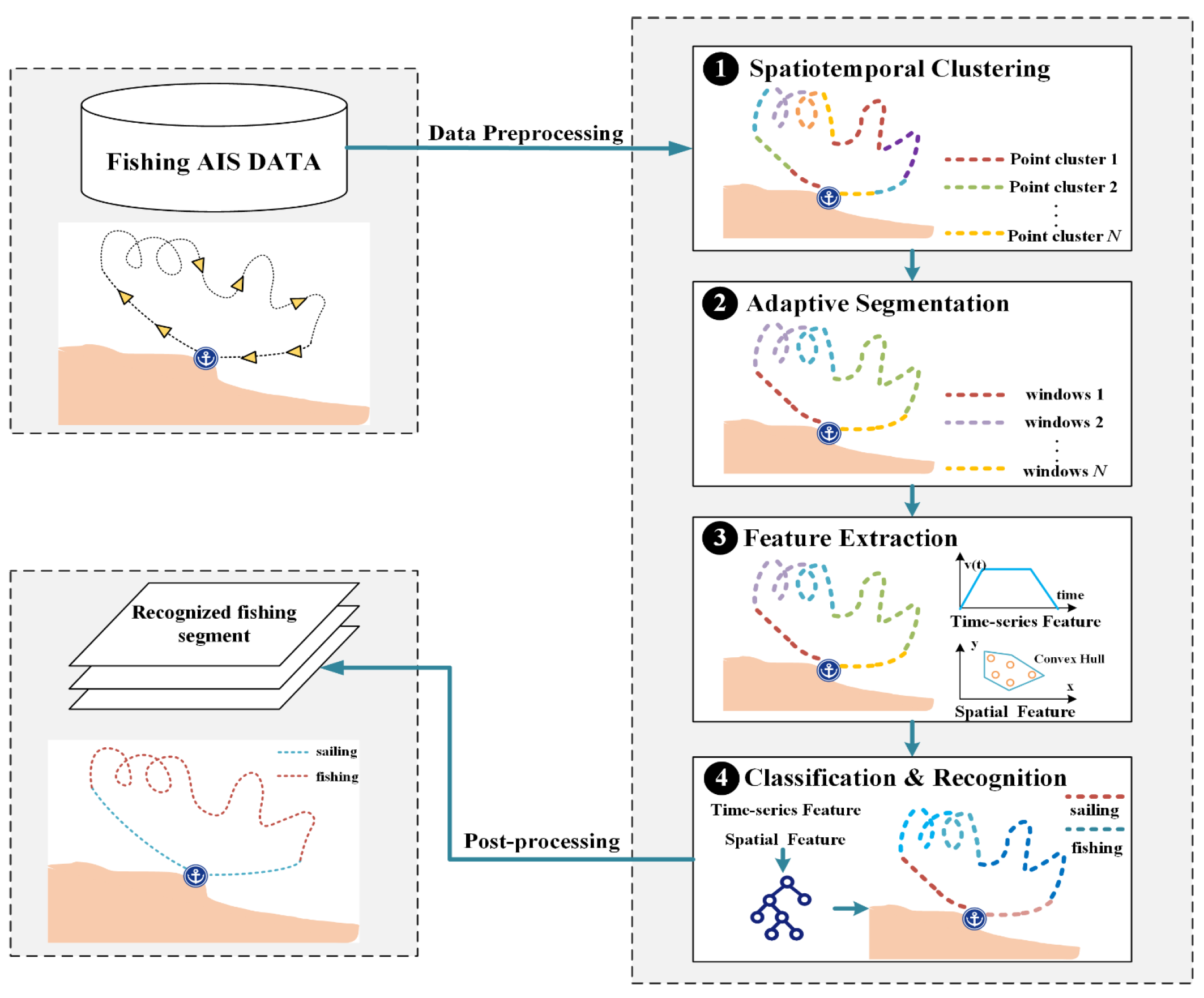
3.3. Spatiotemporal Clustering

Fishing vessel trajectories exhibit high variability, making it challenging to detect patterns. Point-based methods analyze each AIS position independently, failing to capture the continuous nature of fishing operations [25]. Spatiotemporal clustering addresses this limitation by grouping trajectory points based on both spatial proximity and temporal continuity. This approach identifies concentrated fishing areas while preserving the behavioral context essential for distinguishing fishing from transit activities.

Density-based clustering methods, such as DBSCAN, can identify clusters of any shape and handle noise in vessel data [26]. However, DBSCAN only considers spatial attributes. We use ST-DBSCAN, which adds temporal constraints to capture the dynamic nature of fishing activities. This is important because fishing vessels operate in specific areas over extended time periods. ST-DBSCAN has been empirically validated to be well suited for analyzing dynamic spatiotemporal data, such as navigation trajectories [24].

Specifically, we consider a fishing vessel trajectory point sequence P = {p₁, p₂, …, p_i, …, p_n}, where n represents the total number of points in the given vessel trajectory, and each point p_i contains spatial coordinates (x_i, y_i), a timestamp t_i, and other non-spatial attributes (e.g., speed and direction). The ST-DBSCAN algorithm involves three parameters: the spatial radius threshold ε_s, the temporal radius ε_t, and the minimum number of points minPts. Here, points satisfying both spatial (distance ≤ ε_s) and temporal (time difference ≤ ε_t) constraints form neighborhoods. Regions with at least minPts form clusters representing fishing activities, while isolated points are classified as noise, typically indicating transit movements.

To quantify the proximity between vessel trajectory points, we establish a spatial and temporal joint distance metric. Specifically, given two trajectory points p_i and p_j ∈ P, the spatial similarity between p_i and p_j is measured by their geographical distance, while the temporal similarity between p_i and p_j is quantified through their absolute timestamp difference. Then, the spatiotemporal joint distance d_joint between p_i and p_j is thus formulated as follows:

$$d_{joint}(p_i,p_j)\left\{\begin{array}{c}{d}_s=d_{\mathrm{geo}}\left(p_i,p_j\right)\\ d_t=\left|t_i-t_j\right|\end{array}\right.$$

(1)

where d_geo represents the geographical distance (e.g., great-circle distance or projected Euclidean distance) between p_i and p_j, while t_i and t_j denote the timestamp information of p_i and p_j, respectively.

The use of this spatial and temporal joint distance ensures that only adjacent vessel trajectory points exhibiting both spatial density consistency and temporal continuity are grouped together, reflecting real-world fishing activities where vessels conduct localized operations (e.g., trawling within confined areas) over sustained periods. Then, we can use the ST-DBSCAN algorithm to find meaningful clusters from vessel trajectory points. The clustering process is implemented as follows:

Step 1: Denote all vessel trajectory points in P as unlabeled (denoted as P_u).

Step 2: Randomly select an unlabeled point p_i from the set P_u.

Step 3: Compute the spatiotemporal neighborhood N_st(p_i) of p_i by identifying all unlabeled points that satisfy both spatial and temporal proximity constraints relative to p_i, i.e., find all p_j ∈ P_u such that d_s(p_i, p_i) ≤ ε_s and d_t(p_i, p_i) ≤ ε_t. If the number of vessel trajectory points in this spatiotemporal neighborhood of p_i |N_st(p_i)| ≥ minPts, p_i is designated as a core point. Otherwise, repeat Step 2 until a core point is found.

Step 4: Beginning with the identified core point p_i, incorporate all points in its spatiotemporal neighborhood and recursively extend its cluster boundary by traversing the points in its neighborhood and performing Step 3 until no additional points can be added to this cluster.

Step 5: If a point cannot be classified as a core point or is not within the spatiotemporal neighborhood of the core points during the expansion process, it is labeled as a noise point.

Step 6: Repeat Steps 2–5 until all points in P_u have been assigned to a cluster or labeled as noise.

The parameters ε_s and ε_t are crucial for defining the spatiotemporal density thresholds, thus influencing the clustering results. To enhance the adaptability of ST-DBSCAN across diverse scenarios, including varying vessel speeds, vessel types, and meteorological conditions, we propose a data-driven parameter optimization strategy. Specifically, the average spatial distance and the average time interval between consecutive vessel trajectory points within a given vessel trajectory are computed as initial estimates for ε_s and ε_t, respectively. They can be further fine-tuned based on domain-specific knowledge, such as historical fishing ground distributions and user experiences. In this way, the parameters of ST-DBSCAN can be adaptively set according to the inherent characteristics of the specific vessel data without the need for complex parameter search processes.

Dense point clusters in the trajectories of vessels in the results of ST-DBSCAN are labeled as clusters, and sparse clusters are labeled as noise (i.e., cluster label −1). When examining this noise in the context of a time series, we can observe that some subsequences of noise points (i.e., noise segments) in the continuous space have some degree of coherence and persistence over time. These temporal noise segments, despite being labeled as noise due to their sparsity, may represent meaningful fishing patterns. Therefore, to improve the coherence of the segmentation results at the temporal level, we further propose a post-processing step that re-evaluates these noise segments and treats them as independent new clusters.

After clustering, we apply post-processing to improve results. Some consecutive noise points may represent meaningful fishing patterns despite low density. We identify these temporal segments and reclassify them as new clusters when they exhibit temporal continuity and sufficient duration. Specifically, continuous sequences of noise points are promoted to new clusters if they maintain temporal coherence and exceed a minimum duration threshold, ensuring that only persistent behavioral patterns are captured rather than transient movements. This captures fishing activities in less crowded areas or during dispersed operations.

3.4. Trajectory Segmentation

Trajectory segmentation is necessary because fishing patterns may not hold throughout the entire trajectory, but rather in specific parts of it. Traditional methods use fixed-size windows that cannot adapt to varying fishing behaviors. Fixed-window approaches often merge segments with distinct motion patterns, thereby reducing the accuracy of identifying fishing activities. Current adaptive segmentation methods face two key limitations. First, they typically adjust windows based on single parameters, such as speed, missing the multi-dimensional nature of fishing movements. Second, the continuous-valued data in the AIS message requires methods that consider both spatial patterns and temporal continuity simultaneously. Instead of working with individual points, effective segmentation must preserve behavioral coherence across trajectory segments. In addition, when vessel trajectories exhibit diverse spatiotemporal patterns, such as rapid transitions from high-speed navigation to low-speed fishing, a single adaptive criterion often fails to subdivide different fishing behavioral trajectory segments accurately.

Our adaptive segmentation leverages spatiotemporal clusters as fundamental units rather than arbitrary time intervals. The segmentation divides the trajectories into comparable segments by aligning window boundaries with cluster transitions. This approach ensures that each segment captures coherent behavioral patterns identified by ST-DBSCAN clustering, whether representing concentrated fishing activities or transit movements. The method adapts window lengths based on actual vessel activities rather than predetermined thresholds.

Window length thresholds are determined dynamically from trajectory properties. For a trajectory of length L, the initial threshold is set to L/20, balancing segment granularity with computational efficiency. This ratio ensures that there are sufficient data points within each window for meaningful feature extraction, while avoiding over-segmentation. The adaptive mechanism operates by accumulating spatiotemporal clusters until reaching the desired window size. Rather than using fixed-length windows, the algorithm dynamically includes clusters sequentially until the total number of points approaches the threshold. This approach ensures that window boundaries naturally align with behavioral transitions identified by ST-DBSCAN clustering, with each window containing a variable number of clusters depending on their density and size.

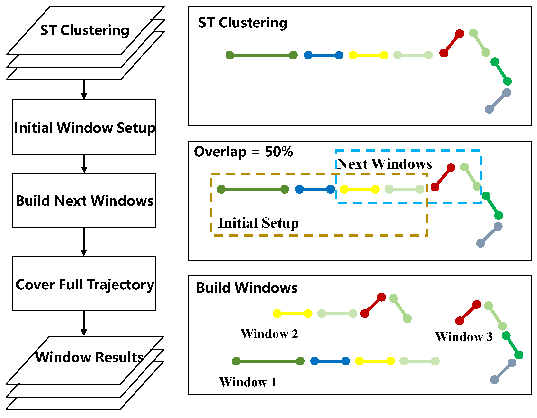
As illustrated in Figure 3, The segmentation process follows four steps. First, trajectory points are organized chronologically with their cluster labels from ST-DBSCAN. Second, windows are constructed by accumulating clusters until the length threshold is reached, starting from the first cluster. Third, subsequent windows incorporate a 50% overlap to maintain continuity between segments, preventing abrupt transitions at window boundaries. Finally, this process iterates until the entire trajectory is covered. To detect complete fishing activities, a run-length encoding technique is used to combine close fishing windows in post-processing.

Using clusters as segmentation units allows the method to account for heterogeneous movement patterns within trajectories. This approach captures both concentrated fishing activities and transitional movements. The adaptive segmentation handles the uncertainty inherent in fishing vessel movements, distinguishing between purposeful fishing operations and random vessel wandering. The result is trajectory segments that correspond to actual fishing behaviors rather than arbitrary divisions.

3.5. Feature Extraction

To classify the trajectories, features are extracted from the tracks, enabling the modeling of ship behavior. Various factors, including vessel performance, hydrological characteristics, and meteorological conditions, influence ship motion. Within each trajectory segment, vessels exhibit distinct patterns during fishing operations compared to transit movements. During a fishing trip, the movement profiles of vessels depend on the activity they are engaged in. Therefore, we extract features that capture both temporal dynamics and spatial patterns to distinguish these behaviors [27]. The multi-dimensional feature enables more accurate classification of fishing behavior compared to single-domain methods, particularly in distinguishing complex fishing operations from transit movements [28]. We therefore select features that directly reflect vessel operational states. The kinematics of ships according to different fishing gears can be effectively classified using movement parameters extracted from each segment. All features are calculated within the adaptive windows to maintain behavioral consistency. Temporal and spatial features provide different but necessary information. Temporal features measure changes in speed and direction over time. Spatial features describe the shape and pattern of vessel movements. Using only one type leads to errors. For example, fishing vessels exhibit similar low speeds during both slow transit and active fishing. However, slow transit typically follows straight paths while fishing operations create curved or repetitive patterns. By analyzing both speed and path shape together, the algorithm can correctly distinguish between these different vessel states. The features used in this study include six main categories.

(1) Velocity Dynamics: This includes average velocity and the frequency of velocity change.

Average velocity: The average velocity in the window represents the overall motion state, calculated as the mean of all velocity values within the window. Straight-line migration behavior tends to have high average velocities, while low average velocities or near-stalling states tend to be low-speed maneuvering for fishing operations.

Velocity change frequency: This metric counts the number of short-term velocity changes, which are likely to be associated with fishing activities. The frequency is calculated as the number of significant velocity changes (where |v_i+1 − v_i| > δ_v) divided by the window duration ΔT. The number of speed changes reflects the ship’s movement in response to the conditions of the fishery and the distribution of the fish school.

(2) Acceleration and steering patterns: This feature class captures the dynamic maneuvering behavior of fishing vessels, such as the volatility of acceleration and the frequency of turning events.

Acceleration volatility: This feature calculates the variability in acceleration patterns. For the provided acceleration sequence $\{a_i{\}}_{i=1}^{b-1}$ within the window, the variance in the acceleration is calculated as follows:

$${\sigma }_a^2={\displaystyle \frac{1}{b-2}}{\displaystyle \sum }_{i=1}^{b-1}{(a_i-\overline{a})}^2$$

(2)

where $\overline{a}$ denotes the average acceleration within the window, and b is the number of trajectory points within the window. Larger acceleration variance indicates frequent correction of fishing vessels’ propulsion, which is consistent with fine-tuning movements during fishing operations.

Turning event frequency: It measures the frequency of directional changes within the window. Given the heading sequence $\{{\theta }_i{\}}_{i=1}^{b-1}$ and a predefined directional change threshold θ_thr, it is calculated as follows:

$$F_{\mathrm{turn}}={\displaystyle \frac{{{\displaystyle \sum }}_{i=1}^{b-1}I(\mathrm{\Delta }{\theta }_i>{\theta }_{\mathrm{thr}})}{\mathrm{\Delta }T}}$$

(3)

where ΔT denotes the time length of the window, Δθ_i = |θ_i+1 − θ_i| represents the absolute difference between adjacent headings, and I(Δθ_i − θ_thr) is an indicator function that equals 1 if Δθ_i > θ_thr and 0 otherwise. Generally, a high number of turning events would imply frequent direction changes in the short term, most commonly corresponding to the repeated circling or maneuvering behaviors of vessels in fishing areas [29].

(3) Low-speed dwelling and temporal features: Two features are utilized to quantify low-speed dwelling behaviors, which are crucial for identifying fishing operations.

Low-speed ratio: This feature calculates the ratio of low-speed points within the window:

$$r_v={\displaystyle \frac{1}{b}}{\displaystyle \sum _{i=1}^{b}I(v_i\le v_{ϵ})}$$

(4)

where v_ϵ is a predefined low speed threshold, b is the length of the speed sequence within the window, and I() is an indicator function that equals 1 if vi ≤ v_ϵ and 0 otherwise. A high value of the low-speed ratio indicates that the vessel is more likely to be conducting slow search or net-casting operations in a specific sea area.

Maximum dwell duration: This feature calculates the maximum duration of continuous low-speed segments within the window, where continuous low-speed segments are identified by the low-speed ratio feature.

$$T_{\mathrm{dwell}}=\max (\{t_i\})$$

(5)

where {t_i} denotes the set of durations for continuous low-speed segments within the window. This feature can effectively discriminate between transient deceleration events and sustained fishing operations through duration-based thresholding. Focusing on continuous low-speed segments rather than isolated points can reduce misclassification caused by sporadic AIS gaps and capture operationally significant dwelling patterns.

In addition to the above temporal features that emphasize motion dynamics, spatial patterns provide complementary information about the fishing behaviors of vessels. Fishing operations often generate distinctive movement patterns, such as repeated turns and complex path shapes within confined areas, which differ significantly from the straight trajectories typical of transit movements. To effectively capture these patterns, we implement a set of spatial features, including geometric morphology, tortuosity, directional complexity, and spatial distribution and compactness features.

(4) Geometric morphology: This type of feature quantifies the global characteristics (i.e., overall shape, structure, and spatial extent) of the vessel trajectory within the window.

Trajectory length: It quantifies the spatial path coverage of a vessel’s movement and can be calculated by accumulating the distance between consecutive points within the window.

$$L=\sum _{i=1}^{b-1}d\left(p_i, p_{i+1}\right)$$

(6)

where d (p_i, p_i+1) denotes the geographical distance between point p_i and its next point p_i+1, and b is the number of trajectory points within the window. Fishing trajectories typically exhibit longer cumulative lengths within localized areas, which are characterized by a higher density of trajectory points due to repetitive search patterns.

Straightness: The straightness index calculates the ratio of the total trajectory length L to the displacement (direct distance between start point p₁ and end point p_b), which can be used to further distinguish linear transit from curved fishing paths.

$$R_{\mathrm{straight}}={\displaystyle \frac{L}{d\left(p_1,p_b\right)}}$$

(7)

When R_straight approaches 1, the vessel trajectory approximates a straight line. When R_straight is significantly greater than 1, this indicates a curved trajectory, which aligns with the meandering pattern generally observed during fishing operations.

(5) Tortuosity and directional complexity: These two features characterize the local path variability (e.g., curvature and turning complexity) of the vessel trajectory within the window.

Local sinuosity: It evaluates the curvature or twistiness of the path by comparing the total path length to the maximum straight-line segment distance within the window, as defined in Equation (8).

$$S={\displaystyle \frac{L}{\underset{1\le j<k\le b}{\max d(p_i,p_j)}}}$$

(8)

where b is the number of trajectory points within the window and L denotes the trajectory path distance within the window.

High sinuosity signifies that the trajectory exhibits multiple turns, windings, and localized dwelling patterns within the spatial domain [30]. Complex fishing behaviors, such as trawling or seine netting, typically result in high sinuosity values due to frequent directional changes and confined movement patterns.

Directional diversity: This metric quantifies the diversity in the heading directions of the vessel. Specifically, the direction space (0~360°) is partitioned into M equal intervals, and the number of trajectory points in each interval is enumerated. Then, the directional distribution entropy is defined to measure the uniformity of directional distribution, as formalized in Equation (9).

$$H_{\theta }=-{\displaystyle \sum }_{\theta =1}^M{\displaystyle \frac{n_{\theta }}{n}}\ln \left({\displaystyle \frac{n_{\theta }}{b}}\right)$$

(9)

where b is the total number of trajectory points within the window, and n_θ is the number of trajectory points whose direction falls within the direction interval θ. High H_θ values indicate uniform directional distribution and frequent turning, which is often associated with fishing operations.

(6) Spatial distribution and compactness features: Two features of the convex hull area and ratio, as well as spatial densities, are used which focus on the spatial distribution and compactness of trajectory points within the window.

Convex hull area and ratio: We construct the minimum convex hull of the trajectory points within the window and compute the area (denoted as A_hull) and perimeter (denoted as P_hull) of the convex hull. Then, the aspect ratio of the convex hull is defined as follows:

$$R_{\mathrm{hull}}={\displaystyle \frac{\underset{1\le i<j\le q}{\max }d(p_i,p_j)}{\underset{1\le i<j\le q}{\min }d(p_i,p_j)}}$$

(10)

where q denotes the number of vertices of the convex hull, and d(p_i, p_j) represents the distance between any pair of vertices of the convex hull.

Fishing activities often involve repeated maneuvering, leading to a relatively compact convex hull, characterized by smaller A_hull values and R_hull values approaching 1.

Spatial density variance: Point density is defined as the number of points falling within a circular neighborhood of radius r centered at a given point. We use the variance in spatial point density to measure the spatial distribution of trajectory points within the window, which is formulated as follows:

$${\sigma }_{\rho }^2={\displaystyle \frac{1}{b}}{\displaystyle \sum }_{i=1}^b{({\rho }_{pi}-\overline{\rho })}^2$$

(11)

where b is the number of trajectory points within the window, ${{\rho }_p}_i$ denotes the density of point p_i, and $\overline{\rho }$ represents the mean density of points within the window. A higher density variance suggests local point clustering within the trajectory, which aligns with the high-density wandering patterns of fishing areas [31].

3.6. Classification and Post-Processing

Vessel trajectory classification requires algorithms that can handle multi-dimensional features while maintaining computational efficiency. Tree-structure-based classifiers generally achieve high evaluation metrics for trajectory-based vessel classification [32,33]. XGBoost is selected as the classification algorithm for this study. The method constructs an ensemble of decision trees using gradient boosting, enabling it to capture nonlinear patterns in vessel movements. The XGBoost and Random Forest algorithms outperformed other methods in classification metrics for this problem. We selected the XGBoost for its computational efficiency and robust performance with multi-dimensional features. The key contributions of STACS lie in the integrated framework that combines spatiotemporal clustering, adaptive segmentation, and comprehensive feature extraction, enabling accurate recognition of fishing activities. The algorithm processes the extracted features from each trajectory segment to predict whether the segment is fishing or non-fishing. Its proven efficiency in handling sparse features, rapid training convergence, and robust generalization have been demonstrated in trajectory analysis and vessel type identification tasks [32,34,35].

During model construction, labeled trajectory subsegments are partitioned into training and validation sets. Formally, the training set comprises M labeled instances $\left\{\right(X_j,y_j){\}}_{j=1}^M$, where $X_j=\left(x_{j1},x_{j2},\dots ,x_{jd}\right)$ denotes the feature vector of the j-th trajectory subsegment, and y_j∈{0, 1} indicates the fishing status (1 for fishing and 0 for navigation). XGBoost constructs an additive ensemble of decision trees by minimizing the following regularized objective function.

$$\mathcal{L}\left(\mathrm{\Theta }\right)={\displaystyle \sum }_{j=1}^{M}l\left(y_j,{\widehat{y}}_j\right)+{\displaystyle \sum }_t\mathrm{\Omega }\left(f_t\right)$$

(12)

where l(.) represents the loss function (e.g., logistic loss), y_j denotes the predicted probability, Ω(f_t) penalizes the complexity of the t-th tree, and Θ encompasses all tree parameters. Through second-order gradient approximation and greedy tree-splitting optimization, XGBoost incrementally improves predictive accuracy while controlling overfitting.

After classification, each trajectory segment receives a binary label indicating whether it is fishing or non-fishing. However, fishing activities can last for hours or even days, and multiple fishing windows likely belong to a single complete fishing activity. Point-based classification often yields fragmented results, where continuous fishing operations appear as alternating segments of fishing and non-fishing activity. Therefore, post-processing is necessary to merge these fragments into coherent fishing episodes.

To resolve transient prediction inconsistencies, run-length encoding (RLE) compresses the label sequence {y₁, y₂, …, y_n} into alternating intervals of consecutive fishing (y = 1) and non-fishing (y = 0) windows.

$$\dots \to a_k^{\left(1\right)}\to b_k^{\left(0\right)}\to c_{k+1}^{\left(1\right)}\to \dots$$

(13)

where $a_k,b_k,c_{k+1}\in {\mathbb{N}}^{+}$ represent the duration (window count) of each interval.

Valid fishing segments are identified via two criteria: (1) Boundary Integrity: Segments must start and end with fishing intervals ($a_k^{\left(1\right)},c_{k+1}^{\left(1\right)}$). (2) Interval Dominance: Non-fishing interruptions $b_k^{\left(0\right)}$ must satisfy the following:

$$b_k\le min\left(a_k,c_{k+1}\right)$$

(14)

This constraint ensures that only brief interruptions are merged while preserving distinct fishing operations. In practice, temporary pauses within a fishing operation are typically much shorter than the fishing activity itself. When a non-fishing period exceeds the duration of adjacent fishing segments, it is more likely to represent a genuine transition between separate fishing operations rather than a temporary interruption. This prevents the over-merging of independent fishing events while effectively reducing fragmentation from operational pauses.

RLE post-processing corrects prediction inconsistencies by merging brief non-fishing segments into surrounding fishing segments when they meet defined criteria. This simple scan extracts continuous fishing segments while identifying non-fishing segments as complementary intervals, ensuring temporal coherence in activity recognition.

3.7. Performance Evaluation

The evaluation examines STACS performance using two datasets with different characteristics. The Danish dataset contains high-resolution coastal trajectories, while the Global Fishing Watch (GFW) dataset provides global-scale vessel movements. Two evaluation levels are used. Point-level metrics measure classification accuracy for individual trajectory points. Segment-level metrics assess the coherence of fishing episodes. This approach evaluates both classification accuracy and the continuity of detected fishing activities, which is essential for practical fisheries management applications.

Specifically, at the point level, we adopt three standard metrics derived from the confusion matrix between ground-truth labels and the predicted labels of fishing activities.

(1) Precision: It is defined as the ratio of the number of correctly classified fishing points to the total number of points predicted as fishing, which reflects the reliability of detected fishing points.

$$Precision={\displaystyle \frac{TP}{TP+FP}}$$

(15)

where TP represents correctly classified fishing points and FP denotes non-fishing points incorrectly classified as fishing points.

(2) Recall: It is defined as the ratio of the number of correctly classified fishing points to the total number of actual fishing points, which measures the ability of the algorithm to detect true fishing activities.

$$Recall={\displaystyle \frac{TP}{TP+FN}}$$

(16)

where FN represents fishing points incorrectly classified as non-fishing points.

(3) F1-score: It is defined as the harmonic mean of precision and recall, which provides a balanced evaluation metric of the algorithm’s ability to identify fishing points.

$$F1-score=2\times {\displaystyle \frac{Precision\times Recall}{Precision+Recall}}$$

(17)

For segment-level evaluation, we quantify semantic coherence through two complementary metrics. Let Θ_T = {θ₁, θ₂, …, θ_T} denote the predicted fishing segments and Ψ_V = {Ψ₁, Ψ₂, …, Ψ_V} represent the ground-truth fishing episodes. We use average purity, average coverage, and their harmonic mean metrics to access segment-level classification quality.

(1) Average Purity (AP): It evaluates internal consistency within predicted segments:

$$AP={\displaystyle \frac{100}{T}}{\displaystyle \sum }_{i=1}^T\underset{j\in \left\{1,\dots ,L\right\}}{max}\left({\displaystyle \frac{N_{i,j}}{N_i}}\right)$$

(18)

where N_i,j denotes the number of points with label γ_j in segment θ_i, L represents the total number of unique ground-truth labels, T denotes the total number of predicted segments, j ∈ {1, …, L} indicates the label index, and i ∈ {1, …, T} represents the segment index.

(2) Average Coverage (AC): It measures how completely each ground-truth fishing segment is captured by the predicted fishing segments, which quantifies the completeness of fishing activities.

$$AC={\displaystyle \frac{100}{V}}{\displaystyle \sum }_{i=1}^V\underset{j\in \left\{1,\dots ,T\right\}}{max}\left({\displaystyle \frac{N_{intersects}\left({\psi }_i,{\theta }_j\right)}{N_i}}\right)$$

(19)

where N_intersects(Ψ_i, θ_j) represents the number of data points that intersect between the ground-truth fishing segment Ψ_i and the predicted fishing segment θ_j, N_i denotes the total number of data points in the ground-truth fishing segment Ψ_i, V is the total number of ground-truth fishing segments, i ∈ {1, …, V} indicates the index of ground-truth segments, and j ∈ {1, …, T} represents the index of predicted segments.

(3) Harmonic Mean (H): It resolves the intrinsic trade-off between purity and coverage and can be calculated as follows:

$$H={\displaystyle \frac{2\times AP\times AC}{AP+AC}}$$

(20)

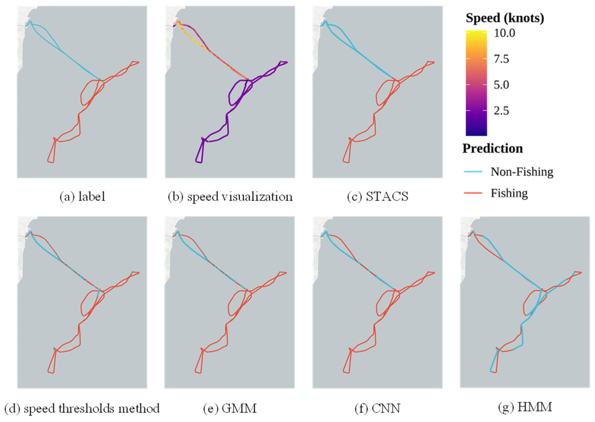
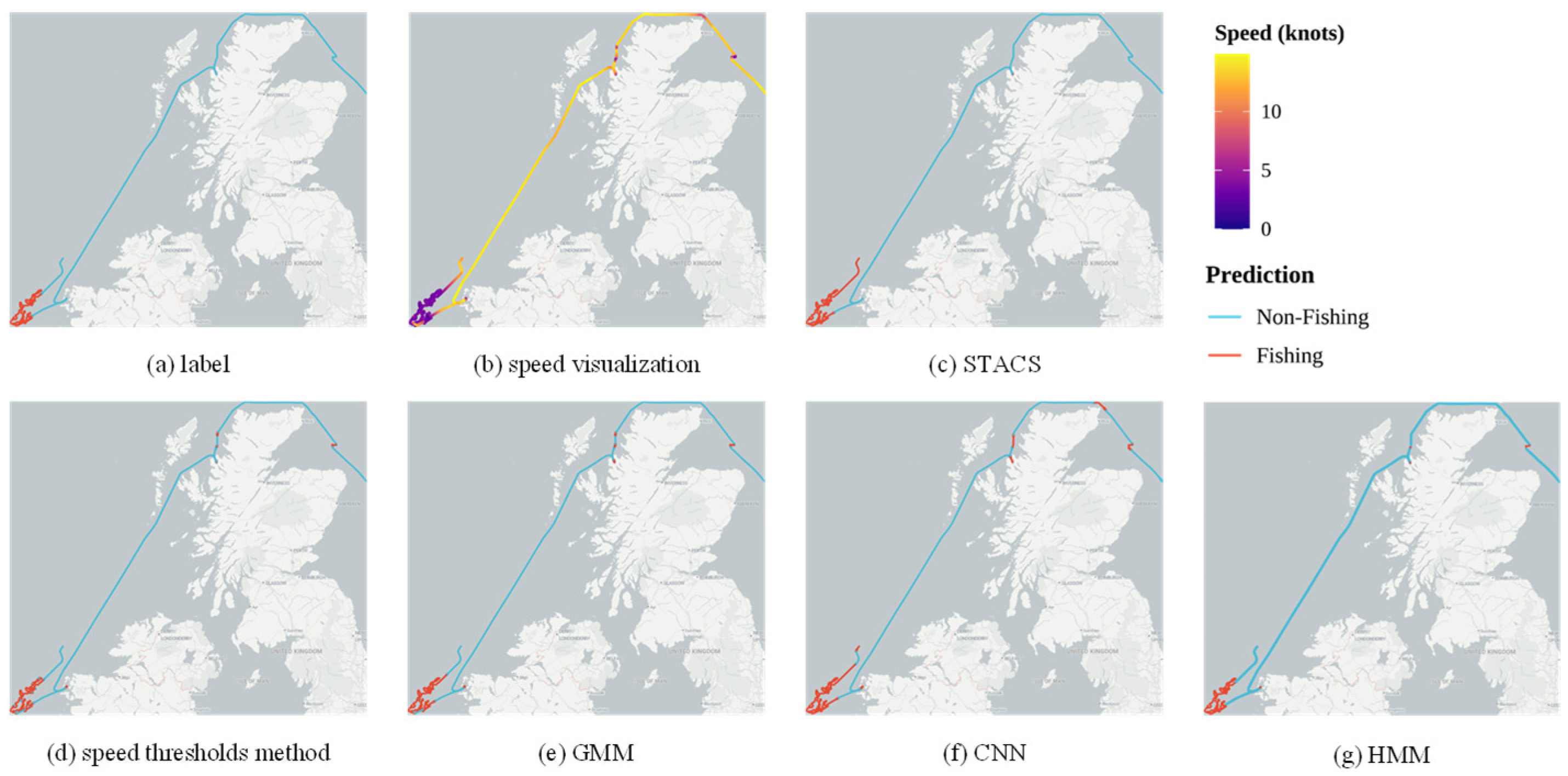
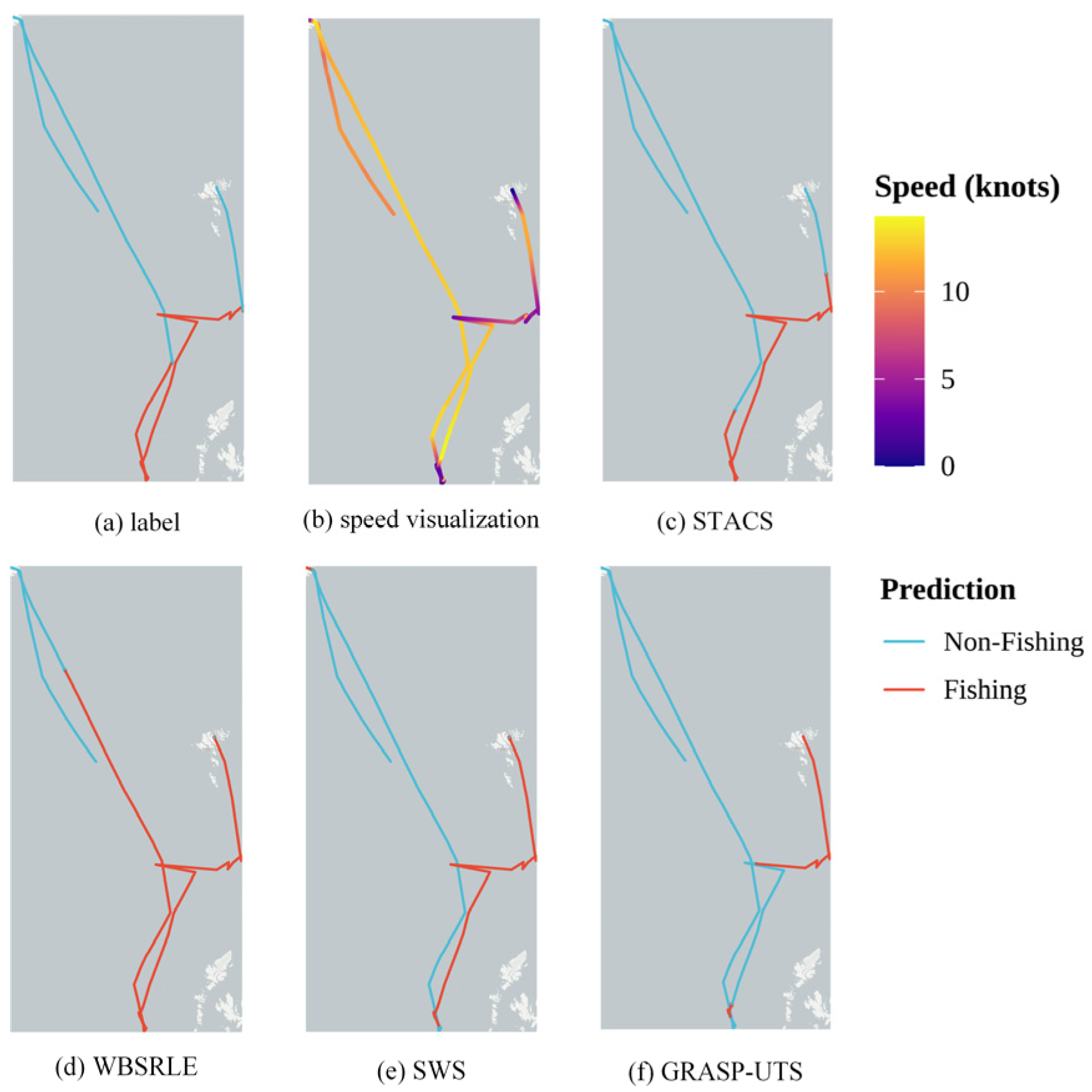
Seven baseline methods are compared to demonstrate the performance of the proposed STACS algorithm. Traditional approaches include speed thresholding (1–5 knots) and Gaussian mixture models (GMMs) for analyzing bimodal speed distributions [16,36]. Advanced methods comprise Hidden Markov Models (HMMs) for state-based behavioral classification using movement parameters [37], convolutional neural networks (CNNs) for spatiotemporal feature extraction, and three segmentation-centric algorithms: GRASP-UTS for multi-objective optimization, sliding window segmentation (SWS), and WBS-RLE, which combines wild binary segmentation with run-length encoding [5,11,14,20].

Experiments are conducted using standardized protocols to ensure comparability. Both the pre-processing pipelines and hardware configurations are identical for all approaches, with trajectories divided by unique vessel identifiers to preserve temporal continuity. This setup enables both instantaneous classification fidelity and operational episode coherence to be stringently assessed on heterogeneous maritime scenarios. Detailed parameter settings and implementation specifications for all baseline methods are provided in Appendix A. While inspired by the original publications, parameters were adjusted to accommodate the characteristics of our dataset and experimental requirements. All processing and computations were performed on an Intel i9-13900K/NVIDIA RTX 4090 platform using Python 3.8 with Pandas and NumPy libraries. The standardized pipeline ensures reproducibility across experiments.

4. Results

4.1. Comparative Performance Evaluation

We evaluated STACS against six baseline methods using both point-level and segment-level metrics across two datasets with distinct characteristics. The Danish dataset represents high-resolution coastal fishing activities, while the GFW dataset captures global-scale oceanic fishing patterns with diverse gear types.

Table 2. Comparative performance of fishing detection methods using point-level indicators.

Dataset	Method	Precision (%)	Recall (%)	F1-Score
Danish data	Speed threshold-based method	94.81	82.05	0.8797
	GMM	94.37	93.97	0.9417
	CNN	94.37	96.13	0.9524
	HMM	74.22	56.97	0.6446
	STACS	95.02	98.92	0.9693
GFW data	Speed threshold-based method	94.60	56.61	0.7083
	GMM	90.91	80.16	0.8520
	CNN	86.89	97.97	0.9210
	HMM	91.06	67.60	0.7759
	STACS	95.63	99.01	0.9729

Bold values indicate the best performance for each metric.

presents the point-level classification performance across all methods. STACS consistently outperformed baseline approaches on both datasets, achieving the highest F1-scores of 0.9693 (Danish) and 0.9729 (GFW). The traditional speed threshold method demonstrated high precision (94.81%) but suffered from low recall (82.05%) on the Danish data, indicating that fishing activities were missed during variable-speed operations. This performance gap widened on the GFW dataset, where recall dropped to 56.61%, highlighting the method’s inability to handle diverse fishing patterns across different gear types and oceanic regions. The GMM achieved balanced precision and recall rates (both exceeding 90%) on the Danish dataset, yielding an F1-score of 0.9417. However, its performance deteriorated on the GFW dataset, with precision dropping to 90.91% and recall to 80.16%, suggesting limited adaptability to heterogeneous fishing patterns. The HMM achieved F1-scores of 0.6446 (Danish) and 0.7759 (GFW), with recall rates of 56.97% and 67.60% respectively. These results suggest that the discrete state-based modeling approach may not fully capture the continuous nature of fishing vessel behaviors, where activities often involve gradual transitions rather than distinct state switches. The higher precision values (74.22% for Danish, 91.06% for GFW) indicate that when the HMM identifies fishing activities, the predictions are relatively reliable, though conservative. The CNN demonstrated high recall (97.97%) on the GFW data but compromised precision (86.89%), resulting in an F1-score of 0.9210. Among all methods tested, STACS achieved optimal performance with a precision of 95.02%, a recall of 98.92%, and an F1-score of 0.9693 on the Danish data, maintaining similar excellence on the GFW data. This demonstrates that STACS, through its spatiotemporal clustering and adaptive segmentation strategies, effectively balances fishing detection rates and false alarm rates while maintaining robustness, even in complex trajectories and varying speed conditions.

Table 3. Comparative performance of fishing detection methods using segment-level indicators.

Dataset	Method	Precision (%)	Recall (%)	F1-Score	Average Purity (%)	Average Coverage (%)	Harmonic Mean (%)
Danish data	WBS-RLE	91.47	99.99	0.9554	89.61	100.00	94.52
	SWS	82.21	95.25	0.8825	90.41	99.98	94.95
	GRASP-UTS	85.29	87.43	0.8634	86.88	100.00	92.98
	STACS	95.02	98.92	0.9693	90.98	99.96	95.26
GFW data	WBS-RLE	89.92	99.41	0.9443	82.62	98.90	90.03
	SWS	86.10	83.33	0.8469	84.75	95.70	89.89
	GRASP-UTS	87.95	55.67	0.6818	83.00	99.29	90.41
	STACS	95.63	99.01	0.9729	85.39	99.52	91.92

Bold values indicate the best performance for each metric.

presents segment-level performance metrics across all methods. WBS-RLE achieved 100.00% coverage on the Danish data but exhibited lower purity (89.61%) and precision (91.47%), indicating over-segmentation, which compromises segment consistency. The unsupervised methods SWS and GRASP-UTS demonstrated variable performance across datasets. These methods achieved adequate coverage under specific conditions but produced inconsistent segmentation when processing trajectories from vessels with different operational patterns. On the GFW data, their F1-scores fluctuated between 0.6818 (GRASP-UTS) and 0.8469 (SWS), reflecting limited adaptability to heterogeneous fishing behaviors.

STACS achieved 90.98% purity, 99.96% coverage, and a 95.26% harmonic mean on the Danish data, maintaining comparable performance on the GFW data (85.39%, 99.52%, and 91.92%, respectively). The method balanced segment purity and coverage across both datasets, outperforming baseline approaches in harmonic mean by 0.31–10.28% on the Danish data and 1.51–24.71% on the GFW data. This performance consistency demonstrates STACS’s effectiveness in preserving behavioral continuity while minimizing segmentation errors across diverse fishing patterns.

To further investigate the contribution of RLE post-processing, we conducted an ablation study comparing STACS with and without this component.

Table 4. STACS performance with and without RLE post-processing.

Dataset	Configuration	Precision (%)	Recall (%)	F1-Score	Average Purity (%)	Average Coverage (%)	Harmonic Mean (%)
Danish data	STACS w/o RLE	93.84	98.32	0.9603	92.65	99.96	96.16
	STACS (full)	95.02	98.92	0.9693	90.98	99.96	95.26
	RLE contribution	+1.18	+0.60	+0.0090	−1.67	0.00	−0.90
GFW data	STACS w/o RLE	92.44	98.98	0.9560	87.42	98.40	92.58
	STACS (full)	95.63	99.01	0.9729	85.39	99.52	91.92
	RLE contribution	+3.19	+0.03	+0.0169	−2.03	+1.12	−0.66

Bold values indicate the best performance for each metric.

presents the detailed comparison. The ablation results reveal that even without RLE, STACS achieves F1-scores of 0.9603 (Danish) and 0.9560 (GFW), substantially outperforming all baseline methods. RLE contributes a 0.90–1.69% improvement in F1-score through smoothing short misclassification sequences. The segment-level metrics show a trade-off: while RLE improves point-level accuracy, it reduces segment purity by 1.67% (Danish) and 2.03% (GFW) due to occasional over-merging of adjacent segments. This trade-off is acceptable given the primary objective of accurate fishing effort quantification. These results confirm that STACS’s core performance stems from its integrated spatiotemporal approach rather than post-processing refinements.

4.2. Visual Analysis of Fishing Activity Detection Results

This section presents visual comparisons of fishing activity detection results between STACS and baseline methods. Point-level methods (speed threshold, GMM, CNN) and segment-level methods (WBS-RLE, SWS, GRASP-UTS) are evaluated using representative trajectories from both Danish and GFW test datasets.

Figure 4 and Figure 5 illustrate how STACS resolved fragmented detection patterns compared to point-level methods on the Danish and GFW datasets. The speed threshold method (Figure 4d) and GMM (Figure 4e) produced scattered results with frequent switching between fishing and non-fishing labels. In contrast, STACS (Figure 4c) maintained continuous segments. For example, in the circular fishing pattern shown in Figure 4, STACS correctly identified the entire slow trawling operation as fishing, while the CNN (Figure 4f) produced broken segments in the same area. This fragmentation issue also appears in the GFW dataset (Figure 5d–g), particularly when vessels slow down near shore, where traditional methods incorrectly classify these slow-speed coastal movements as fishing activities. This contrast underscores the advantage of STACS, which integrates and fuses multi-dimensional features, in mitigating the inherent fragmentation observed in point-level approaches, which ensures meaningful behavioral segmentation that conforms to the logic of fishing operations.

Figure 6 and Figure 7 compare STACS with three segment-level baseline methods. On the Danish dataset (Figure 6), STACS (Figure 6c) correctly identified the fishing segments in the circular pattern while maintaining clear boundaries with transit segments. However, SWS (Figure 6e) and GRASP-UTS (Figure 6f) showed severe over-classification, marking almost the entire trajectory as fishing, including obvious transit movements. WBS-RLE (Figure 6d) performed slightly better but still had some misclassification issues.

The GFW dataset (see Figure 7) reveals different data scenarios. STACS (Figure 7c) accurately separated the long transit segment from the fishing area at the bottom. In contrast, WBS-RLE (Figure 7d) showed over-classification, incorrectly marking the straight transit portion as fishing. Meanwhile, SWS (Figure 7e) and GRASP-UTS (Figure 7f) had worse performances, as they under-classified actual fishing activities by labeling them as transit. These results indicate that fixed-threshold methods often fail to identify the correct segment boundaries. They either merge different activities (over-classification) or fail to recognize continuous fishing operations (under-classification). The proposed STACS method addresses these issues through its adaptive approach, which considers both spatial patterns and temporal continuity. The adaptive clustering groups similar movements together, while the combination of directional consistency and velocity patterns helps distinguish fishing from transit phases. Experiments demonstrate that the proposed method in this paper yields segmentation results that more closely align with actual fishing operations compared to methods employing fixed statistical thresholds.

5. Discussion

This study demonstrates that combining spatiotemporal clustering with adaptive segmentation can effectively enhance the detection of fishing activity from vessel fishing trajectories. The proposed STACS framework achieved an F1-score exceeding 0.96 on both Danish and GFW datasets, outperforming available alternative methods. Compared with previous studies, STACS shows consistent improvements. Kroodsma et al. reported an accuracy of ~90% using a CNN on global AIS data [5]. STACS achieved F1-scores of 0.9693 (Danish) and 0.9729 (GFW), representing a 5–10% improvement. Beyond activity pattern classification, STACS also addresses challenges in ship trajectory segmentation. Wu et al. reported a 92.7% harmonic mean due to over-segmentation issues [11], while STACS achieves 95.26% (Danish). This improvement in ship trajectory segment coherence is crucial for accurately quantifying fishing effort.

The primary reasons for the improvement in classification accuracy of fishing vessel behavior using our method are as follows. First, the ST-DBSCAN clustering algorithm is used to preserve trajectory continuity, addressing a significant limitation of spatial-only clustering which often fragments continuous fishing activities. As demonstrated in Figure 4 and Figure 5, point-based methods yield scattered predictions, whereas STACS maintains coherent segments. By optimizing both spatial and temporal features, our method maintains the integrity of fishing operations across different density regions. Second, the proposed adaptive windowing strategy outperforms fixed-parameter methods like SWS and GRASP-UTS. Figure 6 and Figure 7 demonstrate that conventional segmentation methods yield incorrect segment boundaries, whereas STACS accurately identifies the start and end points of fishing activities. While conventional methods struggle with shifts between fishing operations, our method can dynamically adjust segment boundaries based on local trajectory features, which enhances segment coherence across diverse datasets. Third, the integration of multiple temporal and spatial features that characterize different aspects of vessel fishing behaviors enhances the accurate identification of fishing activities and better differentiates non-fishing activities. Unlike earlier studies that often focus on either temporal patterns or spatial characteristics, the proposed STACS approach considers fishing movement patterns in both dimensions, enabling the detection of complex fishing patterns, such as trawling circles.

Despite the above advancements, two limitations remain that need to be addressed. Firstly, binary classification (fishing/non-fishing) simplifies the variability in fishing activities, considering the difference among various stages of fishing operations. Secondly, environmental factors such as water depth or ocean currents are not considered in our study, which have a non-negligible influence on detecting fishing activity. This is particularly important for gaining a better understanding of fishing behaviors in areas where environmental factors heavily affect fish distribution. Integrating more data sources of ocean currents (e.g., speed, direction, temperature) could aid in classifying different fishing types. Different fishing activity recognition methods are effective in various ocean conditions, and leveraging the advantages of these methods would be beneficial for multi-class classification.

6. Conclusions

This paper presents a novel framework for detecting fishing activities, STACS, which integrates spatiotemporal clustering, adaptive segmentation, multiple feature extraction, and XGBoost classification. STACS addresses three key challenges in fishing activity recognition: trajectory fragmentation, rigid segmentation, and limited feature utilization. Our proposed framework leverages multiple spatiotemporal features and fuses useful information into a robust detection model via an advanced classifier. Comparative experiments were conducted on both coastal (Danish) and global (GFW) datasets and evaluated using both point-level and segment-level indicators. The results demonstrated consistent improvements in both point-level and segment-level metrics over baseline methods. This indicates that STACS effectively identifies fishing activities and preserves fishing behavioral continuity across diverse geographic areas and fishing operations.

By converting raw vessel fishing trajectories into meaningful fishing segments, STACS bridges the gap between trajectory analysis and practical fisheries management. As global fisheries face the pressures of climate change and overfishing, data-driven monitoring becomes increasingly important. In future work, we will focus on identifying more specific types of fishing gear and fishing phases by developing multi-classification methods. More ocean current features (speed, direction, temperature) and ocean environmental data sources, such as water depth, will be integrated for fishing activity classification. Furthermore, the advantages of different methods under various conditions can be fully analyzed and considered, allowing for the development of an integrated method that incorporates multiple strategies to enhance the recognition ability and robustness of existing methods across diverse conditions. Also, we will improve processing efficiency for real-time monitoring applications. These advancements will further strengthen the role of trajectory analysis in supporting sustainable fisheries and ocean management.