Multi-Scale Feature Analysis Method for Soil Heavy Metal Based on Two-Dimensional Empirical Mode Decomposition: An Example of Arsenic

Abstract

The spatial distribution of soil heavy metals was influenced by both natural and anthropogenic factors, and the multi-scale characteristics of heavy metals played a key role in analyzing their influencing factors. Taking arsenic (As) of an oil refining site in Shandong as an example, the As was firstly decomposed into intrinsic mode functions (IMFs) at different scales and a residual using two-dimensional empirical mode decomposition (EMD). Secondly, the spatial variation scales of As, the IMFs, and the residual were quantified by their semi-variograms, respectively. Finally, local spatial correlation analysis and random forest model were employed to analyze the multi-scale features of As, the IMFs, the residual, and environmental variables. The results indicated that the As was decomposed into IMF1, IMF2, IMF3, and a residual using the two-dimensional EMD method, and the corresponding spatial ranges were 72.60 m, 159.30 m, 448.00 m, and 592.36 m, respectively. IMF3 had the highest percentage of variance with a value of 57.56%, indicating that the spatial variation of As was mainly concentrated on a large scale. There were correlations between As and aspect and land use type. However, after the scale decomposition of two-dimensional EMD, there were significant correlations between oil residue thickness and IMF1, land use type and IMF3, land use type, and aspect and residual, respectively. The IMFs and residual had a significant scale–location dependence on environment variables, and the impact of anthropogenic factors on As was mainly reflected at the small and medium scales, while the influence of natural factors was mainly reflected at the large scale. The developed method can provide a methodological framework for the spatial analysis and pollution control of soil heavy metals.

1. Introduction

Soil resources are important components of the earth’s ecosystem, and frequent anthropogenic interference increases pressure on the soil environment. Heavy metal pollution from industrial and mining activities is particularly prominent and has become a key focus of soil pollution prevention and control [1,2]. Large-scale and high-intensity refinery operations discharge substantial waste residue, gases, and wastewater containing heavy metals such as arsenic (As), cadmium (Cd), and lead (Pb) [3]. The disposal of waste residue in the low-lying areas and quarries allows heavy metals to diffuse into and deposit within soil. Similarly, heavy metals in gases and wastewater disperse through the atmosphere and accumulate in the surrounding soil [4]. At industrial waste disposal sites, pH critically controls metal leaching: a low pH dissolves cationic metals, while a high pH mobilizes amphoteric/anionic metals. The waste’s acid neutralization capacity is crucial for buffering pH, though its depletion risks causing pH decline [5]. Spatial heterogeneity generates acidification hotspots, significantly intensifying both spatial variability in metal leaching and environmental risks. During the storage, transportation, and disposal, oil refining waste catalysts undergo leaching, releasing heavy metals such as copper (Cu), nickel (Ni), As, and chromium (Cr) under environmental exposure [6]. The waste generated in the oil refining process is discharged into the soil environment. Due to the irreversibility of potential heavy metal elements, they accumulate and spread in the soil, causing harm to the local environment and human health [7,8]. Implementing the Soil Pollution Prevention and Control Action Plan in China [9,10] aims to strengthen pollution prevention and control efforts, reduce environmental risk costs, and achieve sustainable soil health management. Therefore, investigating the soil heavy metal pollution sources around the refinery is crucial for the subsequent prevention and restoration.

Existing studies primarily examined on-site heavy metal distribution characteristics and sources. An et al. [11] identified smelting and industrial waste as the main sources of As in soil. Deng et al. [12] analyzed spatial distribution characteristics and sources at different depths in copper smelting sites, finding that the average As levels in soil exceeded background values at different depths, while Pb, Cd and As hotspots were concentrated in production areas, with a notably high As near smelting workshops and raw material storage. These studies confirmed that As was a major pollutant with distinct spatial patterns. However, spatial variation results from interactions among natural and anthropogenic factors at different scales, locations, and intensities [13,14]. Scale is a major characteristic of heavy metal pollution, and a scale discrepancy causes a change in the spatial distribution of variables and their spatial relationships [15]. The spatial heterogeneity of heavy metals in soil exhibits a strong scale and location dependence, but the complexity of such multi-scale changes makes it difficult to fit an effective spatial model [16,17]. Given this, it is necessary to deeply explore the variation of heavy metals in soil and its potential influencing factors at different scales. Existing methods for assessing the variability of soil properties at specific scales and locations and the scale-dependent effects on environmental variables mainly include empirical mode decomposition (EMD) [18], wavelet transform (WT) [19], multi-scale kriging nested models [20], factorial kriging [21], and multivariate geostatistical analysis [22]. EMD and WT methods have advantages in processing non-stationary spatial data, and can only analyze the scale variation characteristics of soil properties in one-dimensional spatial sequences. The multi-scale kriging nesting model has advantages in revealing the spatial structure of soil properties and improving the accuracy, but its premise is based on the assumption of stationary data. Factorial kriging allows the decomposition of soil heavy metals into spatial variations of different scales, but can only simulate heavy metal variations within a preset scale range. Multivariate geostatistical methods are also based on the assumption of the stationarity of soil heavy metal variation, while ignoring the spatial scale information of the data. In summary, these methods rely on the stationarity assumptions or preset scales.

However, the variation of soil properties is inherently non-stationary and the scale of variation cannot be preset. Existing studies mainly focus on the spatial variation of soil heavy metals at different scales, but neglect the scale–location variation of soil heavy metals and its response to potential environmental variables. Recently, two-dimensional empirical mode decomposition has been gradually applied to soil science [23,24], which has advantages for processing non-stationary data and the adaptive identification of soil attribute variation scale. Based on the assumption that different simple inherent oscillations at different scales are superimposed on each other, processes occurring in two-dimensional spatial data can be decomposed to separate multi-scale spatial variabilities [25,26]. Therefore, this study selected a refinery in Shandong Province, China, as a case study, and used the key pollutant As element to decompose its spatial variation at different scales. It clarified the distribution characteristics of As at different scales and locations, and identified the influencing factors of environmental variables at different scales, aiming to provide support for the differentiated restoration and treatment of heavy metals for refinery site soils.

2. Materials and Methods

2.1. Study Area

The study area is located in Lixia District, Jinan City, Shandong Province, China, with center coordinates of 117°09′ E and 36°41′ N (Figure 1). The landform type is characterized as a hilly area, with the southern part being a low hilly region and the northern part a sloping plain. The average annual temperature is 14.2 °C, and the annual precipitation is 703.43 mm. The site covers an area of 0.37 km². Due to mountain quarrying in the area, stone pits have formed, and most of the covering layer has been manually removed. The regional surface was developed for the construction of houses and factories, and quarrying backfill was carried out. Waste oil residues were dumped in low-lying areas and stone pits, and oil sludge was distributed in localized areas. Due to frequent human activities, it is crucial to clarify the multi-scale spatial heterogeneity of soil heavy metals at the refinery site.

2.2. Data and Data Processing

The spatial distribution and sources of heavy metals in soil are mainly influenced by both natural and anthropogenic factors [27]. Due to the limited area of the site, the soil type and climate of influencing factors remained essentially invariant in the study area and could not determine the extent of their influence on soil heavy metals. Based on site conditions, data acquisition challenges, soil heavy metal sources, and the influencing factor selection method established by Gong et al. [28], this study selected three natural factors (elevation, slope, and aspect) and three anthropogenic activity factors (land use type, distance to roads, and oil residue thickness) as potential environmental variables affecting As content in soil.

2.2.1. Soil Sample Collection and Analysis

Given the historical dumping areas of petroleum wastes, on-site field surveys, and stakeholder interviews with refinery operational staff, a total of 72 surface soil samples were acquired from April to May 2020, and the spatial distribution of sampling sites is illustrated in Figure 1. Five subsamples were collected from 10 × 10 m quadrat vertices and centroids, and surface soils (0–20 cm depth) were homogenized after removing lithic fragments and biogenic detritus to obtain a 1 kg representative sample for each sampling site. The soil samples were air-dried at 25 ± 2 °C, achieved through agate mortar trituration, and sieved through NIST-certified 2.0 mm stainless steel mesh. The As contents of field samples were then measured using the atomic fluorescence method according to the national standard GB/T 22105.2-2008 in China [29].

2.2.2. Environmental Variables

Using the M210 RTK V2 (DJI, Shenzhen, China) UAV tilt photography technology, remote sensing images that directly reflected the appearance, position, height, and other attributes of the ground objects were obtained from different angles simultaneously. The elevation, slope, and aspect of this refinery site were calculated. Land use type (built-up land and woodland) and road data (width ≥ 2.0 m) were interpreted from remote sensing images, and the nearest-neighbor distance to roads data was calculated using the Euclidian distance tool of ArcGIS 10.8. Oil residue thickness was derived from field investigations. The locations of waste oil residue bottom plate and top plate were obtained by drilling at each soil sampling site, and these measurements were used to calculate the thickness of the oil residue.

2.3. Methods

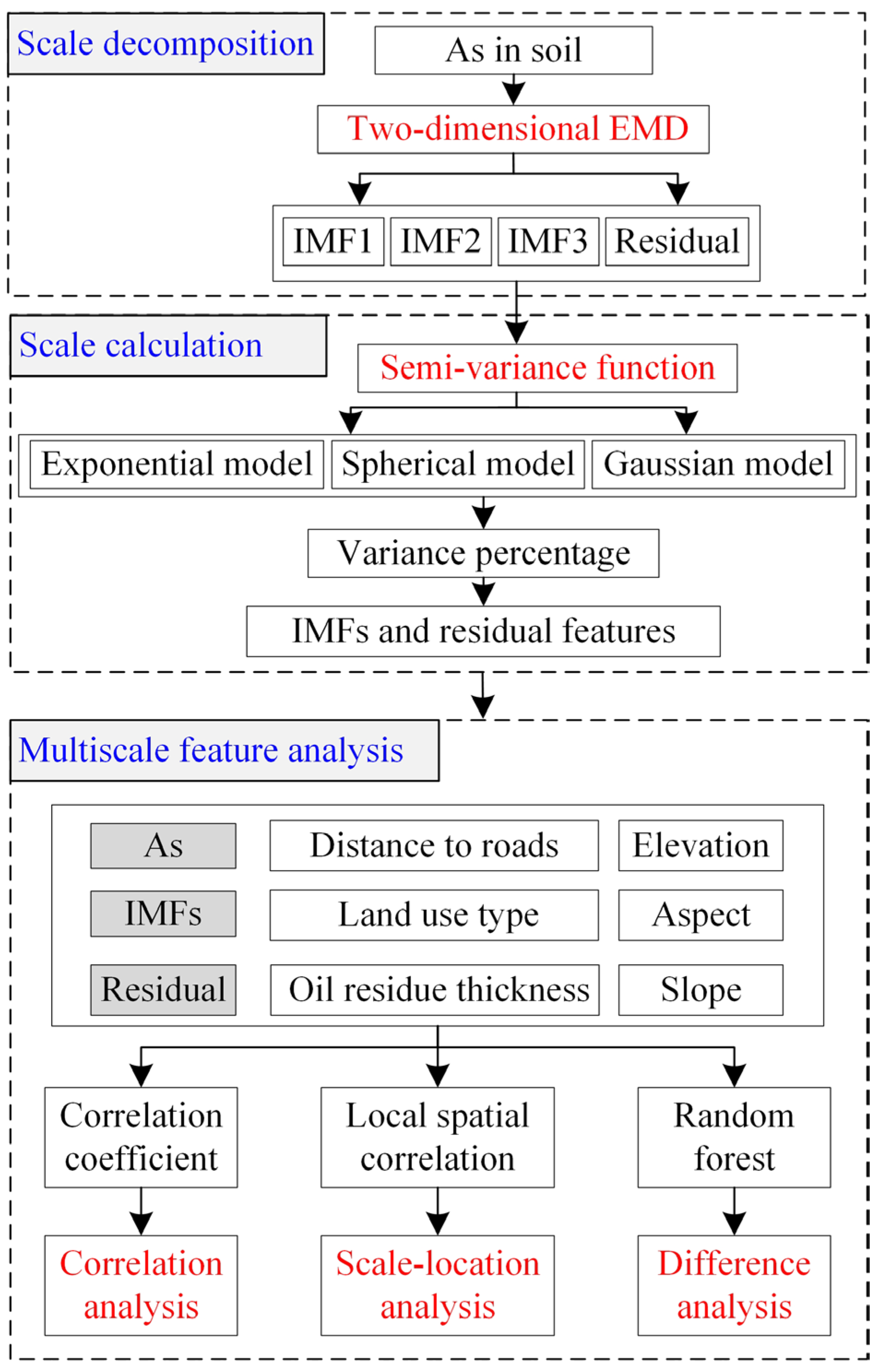
As shown in Figure 2, the technical route was mainly divided into three parts based on scale decomposition, scale calculation, and multi-scale feature analysis. For the scale decomposition part, the two-dimensional EMD method was used to obtain the intrinsic mode functions (IMFs) and residual components representing the spatial variation characteristics of As at a refinery site across different scales. For the scale calculation part, based on the semi-variance function model, the different components from the scale decomposition were fitted to obtain the variation range of heavy metal As at different scales, and the variance percentages at different scales were calculated to determine the main variation scale. For the multi-scale feature analysis part, the main environmental variables affecting As contents were identified by performing correlation analysis, scale–location analysis and difference analysis between As concentrations, the IMFs, the residual component, and the different environmental variables.

2.3.1. Two-Dimensional Empirical Mode Decomposition

Empirical mode decomposition involved the adaptive decomposition of a signal into intrinsic mode functions of different frequencies by extracting the local high-frequency oscillation part of the signal [30]. Two-dimensional empirical mode decomposition was a method used to decompose two-dimensional images or spatial data based on EMD, which can be used to determine the spatial heterogeneity in the scale and location of soil heavy metals [31]. Two-dimensional EMD extracted local oscillations into different intrinsic mode functions and separated the changes within the original data series at different scales. The theoretical mean of the IMFs was 0, and the mean of the residual was equal to the mean of the original data. The decomposition process of two-dimensional EMD was as follows [32,33]. Firstly, the local extreme points of spatial data h_k(x,y) were identified, including the maximum and minimum values. Secondly, the maxima and minima were interpolated to obtain the upper envelope surface and lower envelope surface functions. Finally, the average value of the maximum and minimum values of the interpolation was calculated as the mean envelope surface d_i(x,y). This sifting process continues until the IMF criteria were met, at which point the sifting process was stopped and the residual component was output. The two-dimensional EMD of a spatial dataset is defined as follows:

$$z\left(x,y\right)=\sum _{i=1}^{n-1}{d}_i\left(x,y\right)+r\left(x,y\right)$$

(1)

where z(x,y) is the original two-dimensional dataset; d_i(x,y) and r(x,y) represent the IMFs and the residual, respectively. Usually, the IMF criteria are set between 0.02 and 0.30, while in this study, a value of 0.10 was used, which yielded satisfactory IMFs and the residual.

2.3.2. Semi-Variance Function Model

The semi-variance function model was an effective tool for evaluating spatial variability [34,35,36], which was expressed by the average variance between each pair of points, separated by vector h. The semi-variance is calculated by

$$\gamma (h)={\displaystyle \frac{1}{2N\left(h\right)}}\sum _{i=1}^{N\left(h\right)}{\left[Z\right(x_i)-Z(x_i+h\left)\right]}^2$$

(2)

where γ(h) is the semi-variance; N(h) is the number of soil sampling sites within a distance h; Z(x_i) is the value at a specific point; and Z(x_i + h) is the value at points separated by a distance h. A semi-variogram consists of three basic parameters that describe the spatial structure: $\gamma \left(h\right)=C_0+C$. $C_0$ represents the nugget effect, and $C_0+C$ is total variance (sill). The distance at which the semi-variogram levels off at the sill is called the range.

In the calculation process of the semi-variance function model, common models included the spherical model, Gaussian model, exponential model, etc., and the fitting effect of the model was represented based on the range, R² and variance percentage. In this study, the function model with the highest R² value was selected to determine the range of the different-scale components (IMFs) and the residual for As, representing the dominant scale of spatial variation for the IMFs and the residual. For example, the variable ranges of the three IMFs were ordered from small to large as IMF1, IMF2, and IMF3, corresponding to small-scale, medium-scale, and large-scale variations, respectively, while the residual indicated the overall trend.

2.3.3. Local Spatial Correlation Analysis

Local spatial correlation analysis was used to assess the correlation between two variables within a local spatial range [14]. Based on a moving window, local spatial correlation analysis was performed between soil heavy metal As in different-scale components (IMFs or residual) and environmental variables to produce local spatial correlation coefficient maps between heavy metal As and environmental variables. The calculation formulas for the Pearson correlation coefficient (normal distribution) and Spearman correlation coefficient (non-normal distribution) are shown in Equations (3) and (4), respectively.

$$r={\displaystyle \frac{\sum _{i=1}^n\left(x_i-\overline{x}\right)\left(y_i-\overline{y}\right)}{\sqrt{\sum _{i=1}^n{\left(x_i-\overline{x}\right)}^2\sum _{i=1}^n{\left(y_i-\overline{y}\right)}^2}}}$$

(3)

$$r_s=1-{\displaystyle \frac{6\sum _{i=1}^m{d_i}^2}{m\left(m^2-1\right)}}$$

(4)

where r is the Pearson correlation coefficient; $\overline{x}$ and $\overline{y}$ are the mean values of variables x and y, respectively; x_i and y_i are the ith values of variables x and y, respectively; n is the number of samples; $r_s$ is the Spearman correlation coefficient; m is the number of grades; and $d_i$ is the grade difference of the variables. The larger the correlation coefficient, the more significant the synergistic variation between soil heavy metals and environmental parameters.

2.3.4. Random Forest Method

Random forest (RF) was an advanced statistical method based on machine learning, which used the bootstrap sampling method to randomly extract n samples from the original dataset as a training set. For each bootstrap sample, a decision tree was constructed. Through repeated sampling and training, multiple decision trees were generated to form the random forest [37,38]. Variable importance analysis of random forest provided a robust framework for quantifying the relative contributions of independent parameters [39]. The importance of each parameter on model estimation accuracy was directly quantified using a permutation approach, with lower importance values indicating minor impacts on model performance and higher values reflecting greater influence.

In this study, we only utilized the variable importance evaluations from the RF model, where the importance ranking of environmental variables for the spatial variation of heavy metal As reflected the relative impact of different environmental variables on As. The RF method measured the variable importance using mean decrease accuracy (MDA) [40]. The MDA calculation is shown in Equation (5).

$$MD{A}_r(j)={\displaystyle \frac{1}{T}}{\sum }_t^T\left[{\displaystyle \frac{1}{\left|D_t\right|}}\left({\sum }_{X_i^j\in D_t^i}{\sum }_k{\left(R_k\left(X_i^j\right)-y_i^k\right)}^2-{\sum }_{X_i\in D_t}{\sum }_k{\left(R_k\left(X_i\right)-y_i^k\right)}^2\right)\right]$$

(5)

where T is the number trees in the RF, $X_i^j$ denotes the feature vector where the jth feature of X_i is randomly permuted; D_t is the out-of-bag sample set for tree t; R_k(X_i) is the predicted value for the kth output dimension of sample X_i; $y_i^k$ is the true value for the kth output dimension of sample i; and k is the number of output dimensions.

3. Results

3.1. Two-Dimensional Empirical Mode Decomposition of As

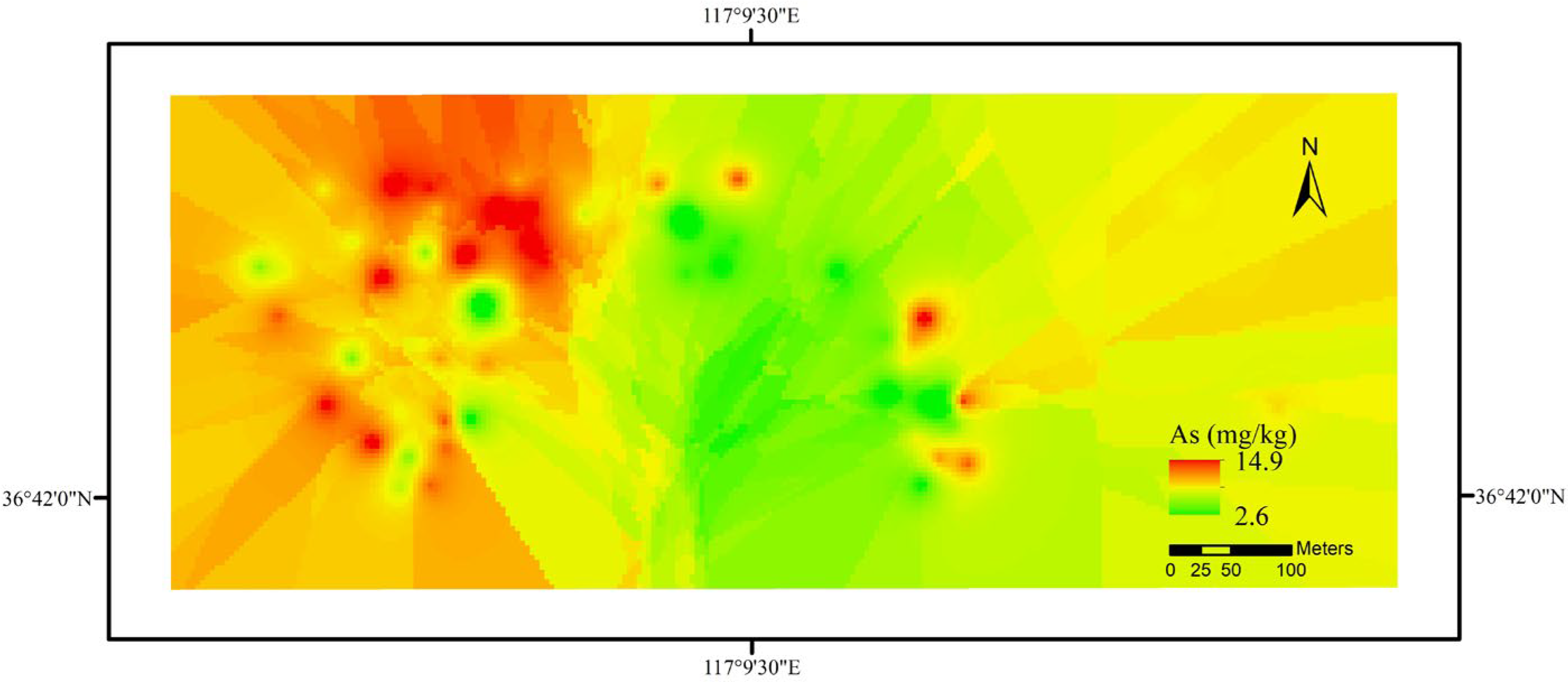
Based on soil samples, the lowest concentration of heavy metal As at the refinery site was 2.6 mg/kg, while the highest concentration was 14.9 mg/kg, with an average concentration of 10.1 mg/kg. None of the As concentrations in the samples exceeded the risk screening value (60 mg/kg, GB 36600-2018) [41]. However, 33 samples had As concentrations exceeding the background value for Jinan soil (10.4 mg/kg) [42], accounting for 45.83% of the total samples, indicating the significant accumulation of As in the refinery site soil. The inverse distance-weighted interpolation of As concentrations in the 72 soil samples was performed, and the results are shown in Figure 3. High concentrations of As were located in the northwest part of the study area, while lower concentrations were mainly distributed in the central part, showing a spatial distribution pattern of higher values in the west and lower values in the east.

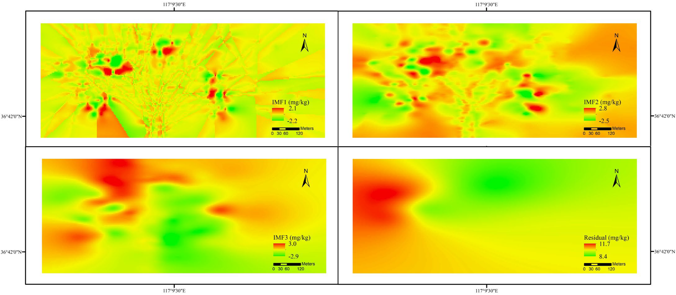
Based on two-dimensional EMD, soil heavy metal As was decomposed into intrinsic mode functions (IMF1, IMF2, IMF3) and a residual component (Figure 4). The spatial distribution of heavy metal As varied significantly across different scales. The variated range of IMF1 was between −2.2 and 2.1 mg/kg, with high and low values distributed in spots. The IMF2 ranged from −2.5 to 2.8 mg/kg, with high values distributed in the built-up areas of the study site. The IMF3 ranged from −2.9 to 3.0 mg/kg, with high values in the northeast building areas and low values in the central and southern wooded areas. The residual ranged from 8.4 to 11.7 mg/kg, reflecting the overall trend of heavy metal As variation. The spatial variation of As changed with scale: IMF1 and IMF2 exhibited fragmented distributions and pronounced local variations, whereas IMF3 and the residual showed continuous distributions. The original scale of As spatial distribution was most similar to IMF3, indicating that dominant variation occurred at this scale.

3.2. Characterization of Intrinsic Modal Functions and Residual

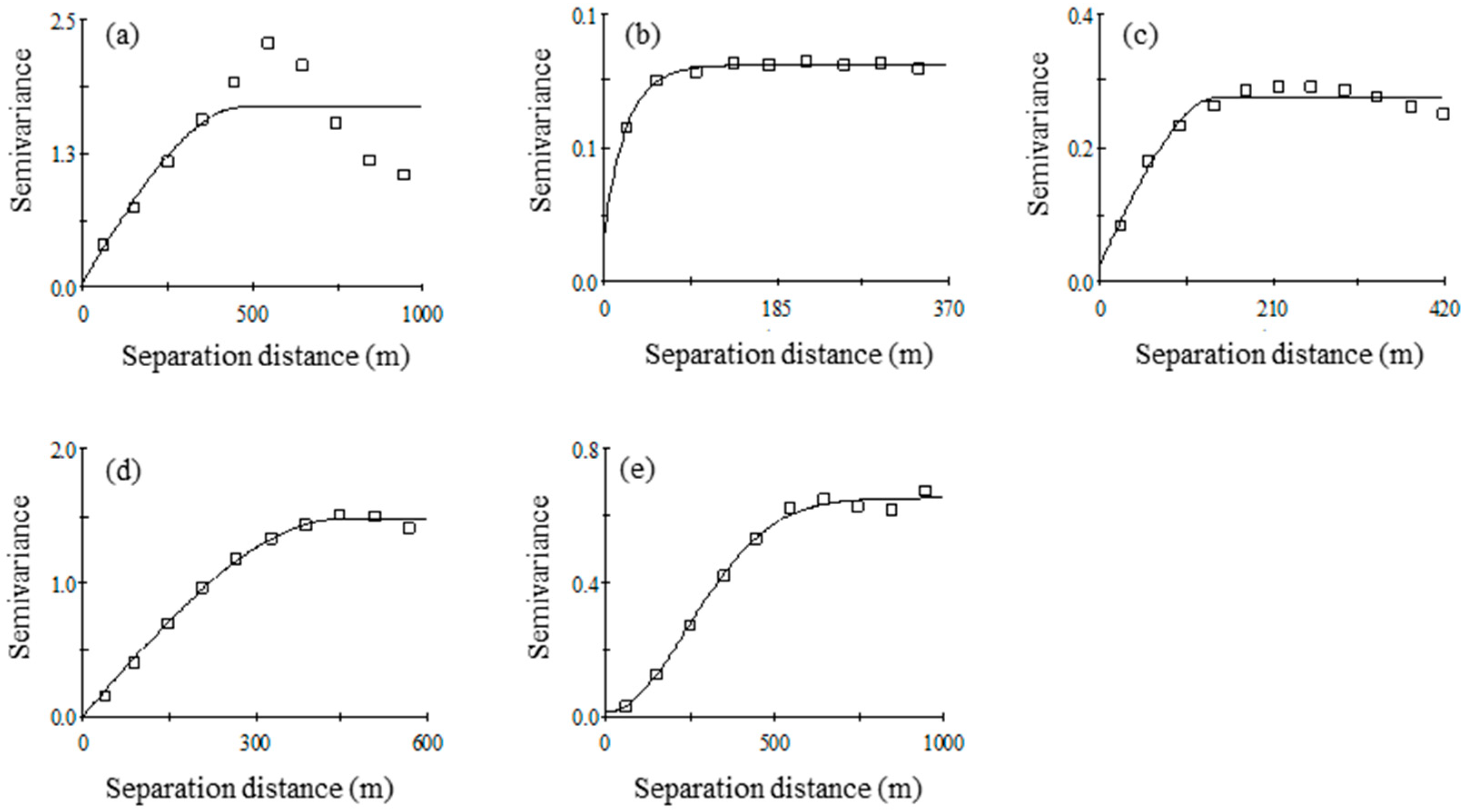
The spatial variability of the original As, IMFs, and the residual was quantified using the semi-variance function, and the optimal fit functions are shown in

Table 1. Optimal semi-variance function models for original As, IMFs, and residual.

Parameter	Model	Separation Distance (m)	R2	Variance Percentage (%)
As	Spherical	466.00	0.61	100
IMF1	Exponential	72.60	0.98	3.72
IMF2	Spherical	159.30	0.97	14.13
IMF3	Spherical	448.00	0.99	57.56
Residual	Gaussian	592.36	0.97	24.59

. The results indicated that the variability scale gradually increased from IMF1 to IMF3, and the residual represented the largest scale of spatial variability for As, which could not be decomposed further. The range of the semi-variance function for the original As at the original scale was 466.00 m (R² = 0.61, Figure 5a), indicating that the spatial variability scale of As was 466.00 m. The variability scale of component IMF1 was fitted by an exponential model (R² = 0.98, Figure 5b), and the semi-variance function showed that the spatial variability scale of IMF1 was 72.60 m. The variability scale of IMF2 was fitted by a spherical model (R² = 0.97, Figure 5c), with a spatial variability scale of 159.30 m. The variability scale of IMF3 was also fitted by a spherical model (R² = 0.99, Figure 5d), with a spatial variability scale of 448.00 m, which was close to the variability scale of the original As. The variability scale of the residual was fitted by a Gaussian model (R² = 0.97, Figure 5e), with a spatial variability scale of 592.36 m. Based on the range sizes, the IMF1, IMF2, and IMF3 were defined as small, medium, and large scales, respectively. The variance percentage of As spatial variability at different scales to its original spatial variability was in the order of IMF3 > residual > IMF2 > IMF1 (Table 1). The two-dimensional EMD extracted IMF components that matched the local spatial oscillation scale through iterative screening. The IMF3 range (448.00 m) derived from the semi-variance function was highly consistent with the original As variation scale (466.00 m) and IMF3 had an optimal determination coefficient (model fit). Consequently, IMF3 accounted for 57.56% of the variance, indicating that As variability predominantly occurred at large scales.

3.3. Analysis of Environmental Variables Influencing Heavy Metal As

3.3.1. Correlation Analysis Between As, IMFs/Residual, and Environmental Variables

Based on the distribution characteristics (normal distribution or non-normal distribution) of environmental variables, the correlation between As and elevation, slope, aspect, distance to roads, and oil residue thickness was calculated using the Pearson correlation coefficient (Equation (3)), respectively, while correlation with land use type was calculated using Spearman correlation coefficient (Equation (4)). The results are shown in

Table 2. Correlation coefficients between original As and environmental variables.

Environment Variables	Elevation	Slope	Aspect	Distance to Roads	Land Use Type	Oil Residue Thickness
Correlation coefficient	−0.05	0.04	−0.28 *	0.22	−0.35 **	−0.18

** Significant at the 0.05 level; * Significant at the 0.1 level.

. Heavy metal As showed significant correlations with aspect and land use type. No other environmental variables showed significant correlations at the original scale, indicating that the spatial variability of As was mainly influenced by aspect and land use type at the original scale.

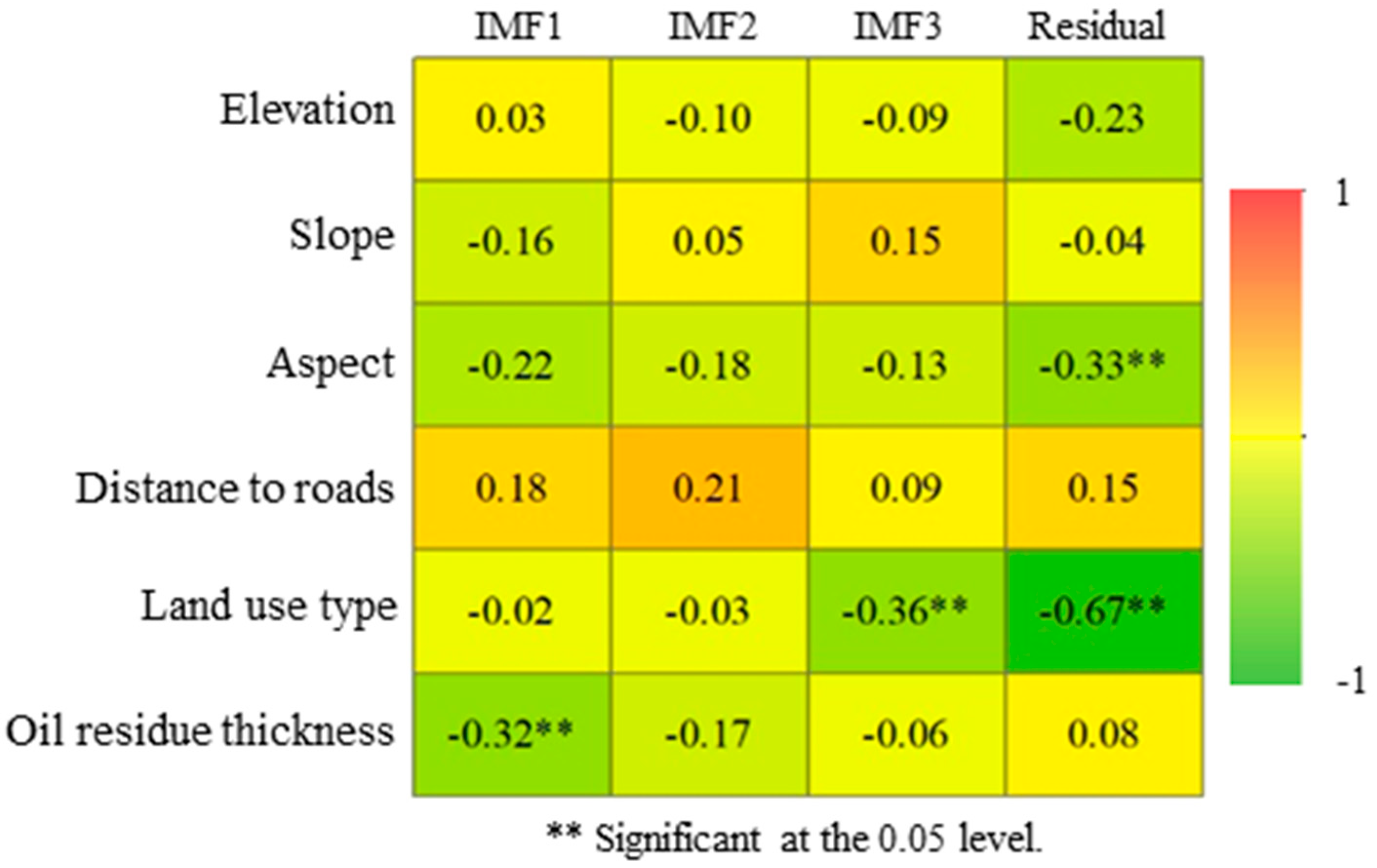
After scale decomposition using two-dimensional EMD, correlations between IMF1, IMF2, IMF3, residual, and environmental variables were determined, as shown in Figure 6. The correlations between small-scale IMF1, medium-scale IMF2, large-scale IMF3, the residual, and environmental variables were not consistent with the correlations between the original As and environmental variables (Table 2, Figure 6). Specifically, aspect was significantly correlated with As at the residual scale, but no significant correlations were achieved at other scales. Land use type showed a significant correlation at the large-scale IMF3 and the residual, with a particularly strong correlation with the residual, indicating that land use type mainly influenced the spatial variability of As at a large scale. The correlations between medium-scale IMF2 and environmental variables were not significant. After scale decomposition, oil residue thickness was significantly correlated with small-scale IMF1, while the influence of oil residue thickness on As was not identified at the original scale.

3.3.2. Scale–Location Analysis of IMFs/Residual and Environmental Variables

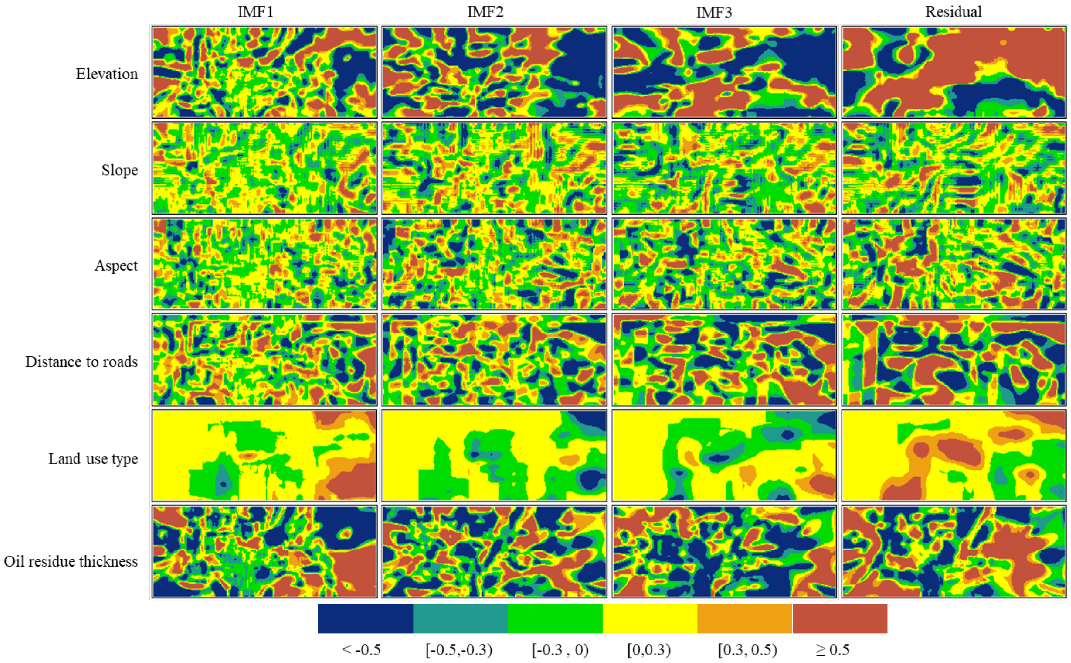
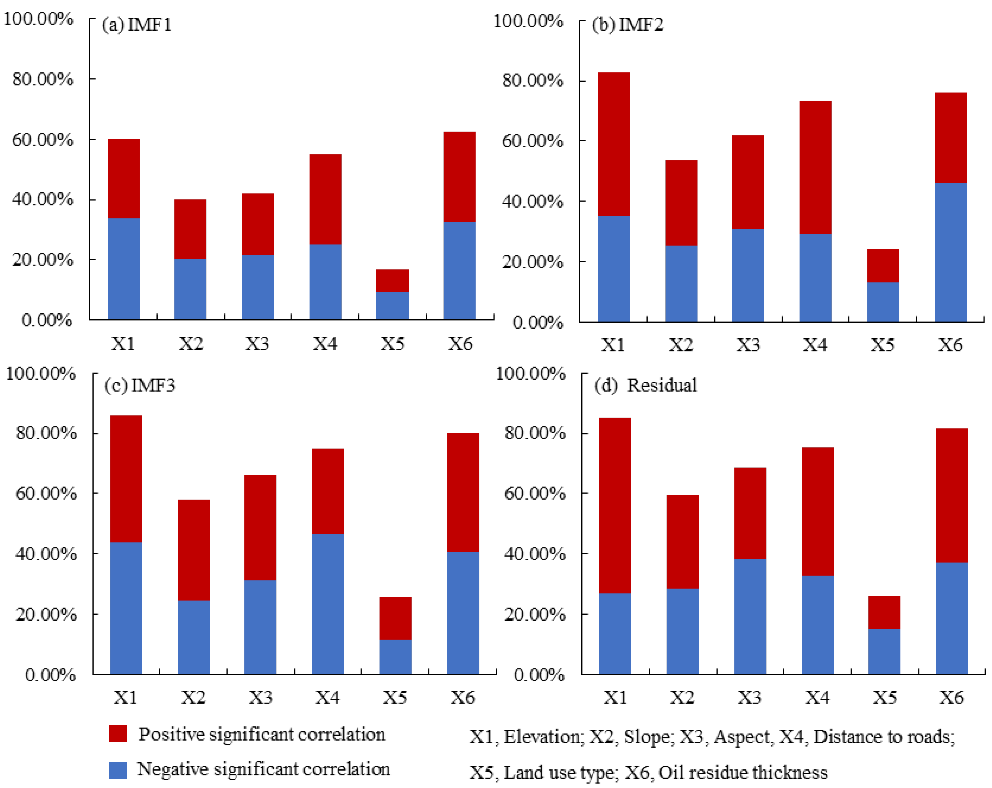
The local spatial correlations between IMFs/residuals and environmental variables are shown in Figure 7. The correlations between environmental variables and As exhibited clear scale–location dependency, meaning their impacts on As varied with both scale and spatial heterogeneity. Figure 8 illustrated the proportion of area with significant correlations between each environmental variable and IMFs or residual. For small-scale IMF1 (72.60 m), oil residue thickness and elevation had significant correlation coverage with IMF1, accounting for 62.61% and 60.18% of the area, respectively (Figure 8). These were the primary drivers of As variability at this scale. For medium-scale IMF2 (159.30 m), In addition to oil residue thickness and elevation, distance to roads also showed significant correlation coverage with IMF2, with a proportion of 69.76%. For large-scale IMF3 (448.00 m) and residual (592.36 m), the significant correlation coverage for all environmental factors increased progressively, indicating strengthening correlations at larger scales. Slope and aspect exhibited significant correlations (r = 0.3–0.5; Figure 7), while elevation, distance to roads, and oil residue thickness showed stronger significant correlations (r > 0.5; Figure 7).

3.3.3. Difference Analysis in Environmental Variables Influencing As, and IMFs/Residual

The differences in the impact of environmental variables on heavy metal As were reflected through the relative importance results of the random forest model. The random forest model revealed that the influence of natural factors and anthropogenic factors on As variability was relatively similar at the original scale, accounting for 49.51% and 50.49%, respectively (Figure 9a). These results indicated that both natural and anthropogenic factors jointly influenced the As variability at the original scale. At different scales, the influence of natural and anthropogenic factors on As variability showed differences. For small- and medium-scale components of As (IMF1, IMF2) and the residual, anthropogenic factors had larger proportions of influence. Conversely, for the large-scale component (IMF3), natural factors dominated (77.17% vs. 22.84%), as suggested in Figure 9b. At a medium scale (IMF2), anthropogenic factors accounted for 60.25%, which was a greater proportion of natural factors (39.75%). At a large scale (IMF3), natural factors comprised 77.17%, which was more than three times the proportion of anthropogenic factors (22.84%) (Figure 9b).

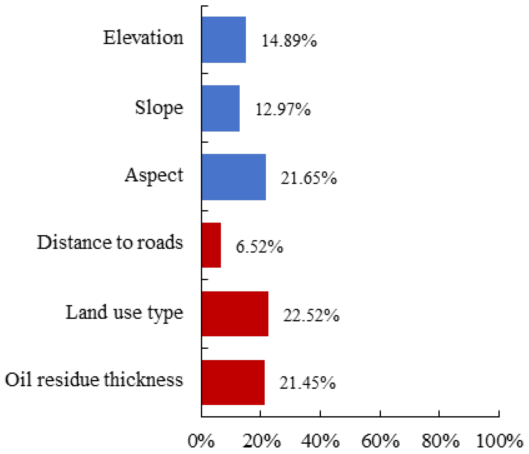
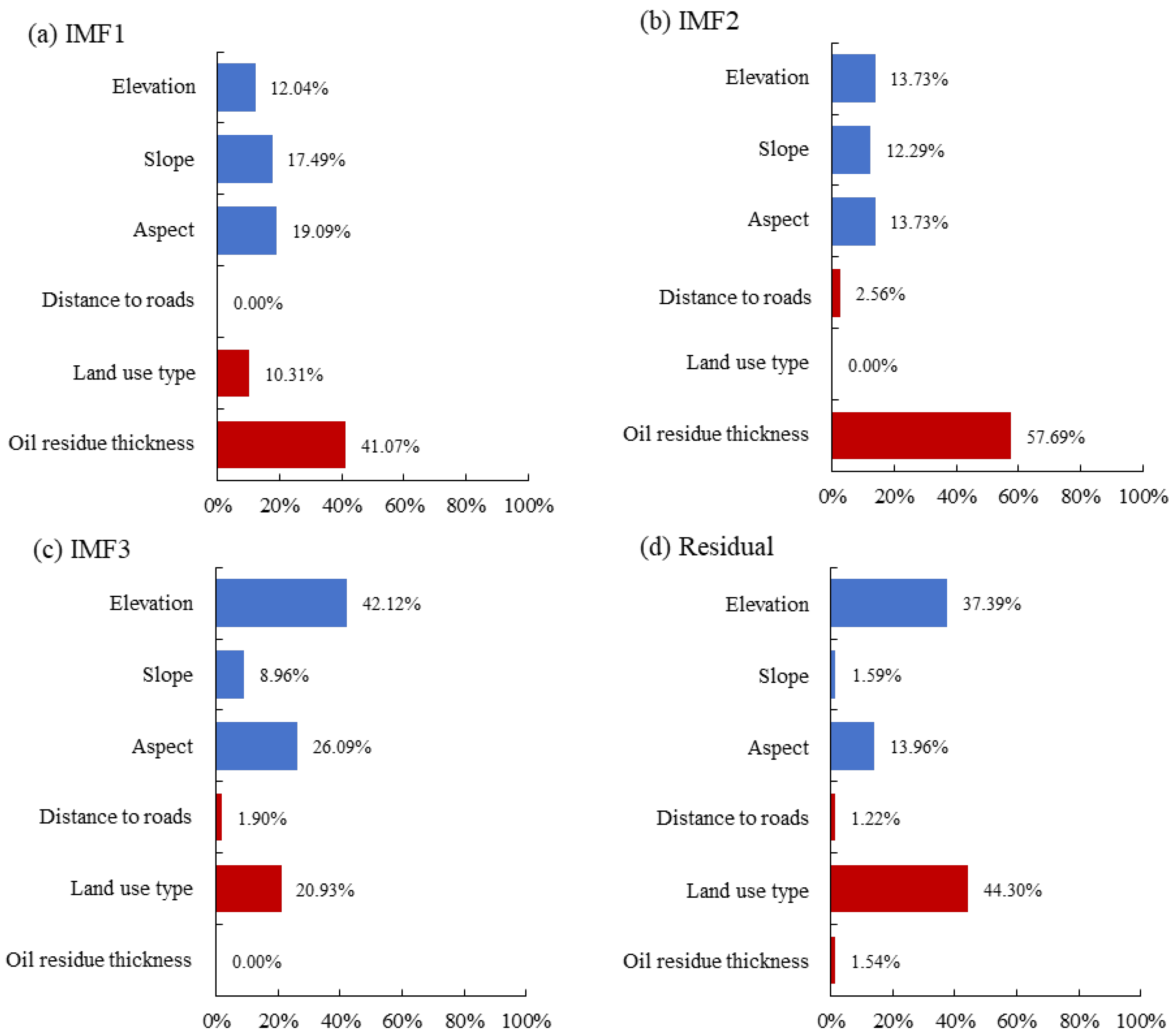
Figure 10 and Figure 11 show the differences in each environmental factor’s impact on As, IMFs/residual variability, respectively. The results indicated that the contribution of each factor ranged between 6.52% and 22.52% at the original scale, with land use type, aspect, and oil residue thickness having relatively greater influence. For small-scale IMF1 (Figure 11a) and medium-scale IMF2 (Figure 11b), oil residue thickness accounted for 41.07% and 57.69%, respectively, indicating that oil residue thickness was the dominant factor influencing As variability at small and medium scales. As scale increased, the contributions of elevation and aspect (natural factors), and land use type (anthropogenic factor) increased significantly. However, the influence of land use type on As variability was less than the combined effect of elevation and aspect, suggesting that elevation and aspect were the dominant factors influencing the spatial variability of As at large scale (IMF3). Residual-scale variability was primarily driven by the interaction of elevation, aspect, and land use type. In summary, the influence of environmental factors on As variability showed significant differences across different scales.

4. Discussion

4.1. Comparisons with Related Studies

Considering the refinery’s development history and specific context, this study comprehensively compared the multi-scale characteristics of As in soil with existing studies. The refinery in the study area was established during the Ninth Five-Year Plan period in China, with a long history of producing gasoline, diesel, and fuel oil. Over thirty years, significant changes occurred in topography and land use. Four original waste oil residue disposal sites (depressions/quarries) were backfilled, covered, and repurposed. This dumping caused spatial heterogeneity in As distribution, with distinct variations across different-scale components (IMFs). Previous studies indicated that the residual represented the overall spatial trend of soil properties [17]. In this study, land use type primarily governed the spatial variations of IMF3 and the residual for As, showing a particularly strong correlation with the residual (Figure 6). According to Figure 11, land use type accounted for 20.93% of the variation in IMF3 and 44.30% of the residual spatial variation, respectively. This indicates that land use type predominantly influenced the large-scale spatial patterns of As. The transition between high and low residual values of soil As was consistent with the distinction between developed and undeveloped land, further indicating that the As variation trend reflected differences between these land use types. Additionally, variability scales increased progressively from IMF1 to residual, consistent with prior findings on the two-dimensional spatial characteristics of soil properties [14,32].

The spatial distribution of soil heavy metals was primarily influenced by factors such as topography, climate, vegetation, anthropogenic activities, and soil-forming factors. Previous studies often analyzed the impact of single environmental factors on the accumulation of soil heavy metals by controlling variables or using global correlation coefficients to represent the relationship between heavy metals and environmental factors [32]. However, the spatial correlation between environmental factors and heavy metal As varied across different scales and locations in this study, indicating that the relationship was not singular but changed with scale and location. Given the small study area, limited slope/aspect variations resulted in minimal influence on As, especially in the local regions. Elevation showed large significant correlation areas across scales, indicating microtopography’s crucial local role. While prior research suggested that heavy metals accumulated in low-lying areas [43], this study found no consistent low-elevation enrichment trend across As scales. This was mainly due to the small differences in elevation within local areas, and the significant randomness in As migration and diffusion, factors responsible for the impact of elevation on heavy metals complexes. Road transport of refinery waste caused As pollution near roads through pollutant deposition [44]. The positive correlation between As and distance to roads was only significant in large-scale IMF3 areas, indicating that As enrichment decreased with increasing distance to roads. Waste oil residue thickness showed large significant correlation areas across scales. Field investigations revealed the site was originally a limestone quarry where waste oil was dumped in depressions/pits. Weathering and rainwater erosion accelerated heavy metal migration, creating identifiable point-source pollution in local areas. Additionally, the significant correlation zones between As and land use type were small across all scales. Significant correlation was only observed in certain developed areas, due to frequent anthropogenic activities, such as wastewater and exhaust emissions, making heavy metal pollution, which was consistent with existing findings [45,46]. Furthermore, the significant correlation area between As’s small-scale component (IMF1) and environmental variables was notably smaller than other scales. This suggested small-scale As variability may be governed by microscale soil properties or formation processes, highlighting the need for further investigation into microscopic mechanisms.

4.2. Advantages and Limitations for Analysis Results of Different Methods

The results of correlation analysis and local spatial correlation analysis diverged substantially, which was consistent with findings by Zhu et al. [14] and Zhou et al. [31]. Taking elevation as an example, the results of correlation analysis showed that the correlation between elevation and IMFs/residual of As was not significant, while the local spatial correlation analysis results revealed that elevation significantly affected the spatial differentiation of As at different scales. This discrepancy likely arises because soil properties integrate complex geographic and formation processes operating at different scales, where environmental variables exert varying magnitudes and mechanisms of influence across regions. In addition, local spatial autocorrelation may exist in both heavy metal As and environmental variables, making localized analysis more reflective of true relationships. However, local spatial methods may also neglect environmental variables with minimal local variation, and subtle effects within limited spatial ranges. For example, the local spatial correlation analysis of land use type on As in this study showed completely insignificant results in the contiguous construction areas in the west and north-central regions, and the significant effects of land use type on As variation were much smaller than those of the other factors in terms of the area of significant correlation zones. Therefore, advantages and limitations of different methods should be considered, and a comprehensive evaluation should be conducted.

Random forest results reflected environmental variables’ relative influence on As but not directionality (positive/negative). The differences in the impact of natural and anthropogenic factors on the variation of As at different scales (Figure 9) indicated that natural and anthropogenic factors jointly controlled As variability at the original scale. After scale decomposition, (1) anthropogenic factors dominated at the medium-scale IMF2; (2) natural factors dominated at the large-scale IMF3; and (3) both natural and anthropogenic factors jointly governed the variation at the small-scale IMF1 and residual. For the single factor, oil residue thickness had the largest impact at the small-scale IMF1 and medium-scale IMF2, which was consistent with the results of the local spatial correlation analysis. Oil residue thickness dominated As variation at the small and medium scales. For large-scale IMF3 and residual component, the random forest model detected elevation’s effect on As; however, like correlation analysis, it failed to capture local impacts of waste oil residue thickness and distance to roads on As. Both the random forest and correlation analysis methods can reflect the association relationship between environmental variables and As in the whole area. The random forest model can also reflect the differences in the effects of environmental variables on the As variation and rank the effect sizes. However, both methods ignore the relationship between environmental variables and As in the local area, while local spatial correlation analysis effectively identifies location-specific impacts of environmentally dynamic variables on As. Therefore, integrating these approaches provides more accurate foundations for site-specific remediation strategies at future refinery sites.

4.3. Multi-Scale Determination Method for Spatial Variability of Soil Heavy Metals

The spatial distribution of heavy metals in soil manifested multi-scale heterogeneity due to the interactions between geopedological matrices and cross-scale environmental drivers. Determining the scales for spatial variability of soil heavy metals was critical and challenging. Traditional methods for scale determination mainly included two types. Firstly, empirical analyses were conducted at basin, county, or site levels to analyze the impact of environmental factors on the spatial heterogeneity of soil heavy metals within various spatial extents [47]. Secondly, resampled grid pixels of environmental factors with different sizes were used to analyze their effects on the spatial heterogeneity for soil heavy metals at different scales [32]. However, those methods could not accurately capture the nonlinear and non-stationary spatial variations of soil heavy metals. To address this challenge, the proposed two-dimensional EMD method had significant advantages in handling non-stationary and nonlinear spatial data. The method identified effectively the scales for spatial variation of heavy metals in soil (Table 1 and Figure 5), and accurately obtained the scale effects and influencing factors for spatial variation of heavy metals in soil.

For future implementation, we developed a technical specification outlining appropriate methodologies and procedures for multi-scale feature analysis, and also provided recommendations for the effective global application of this approach. When deploying the proposed method across diverse environmental contexts worldwide, localization adjustments must account for variations in data sources, study scales, and research targets.

5. Conclusions

This study proposed a multi-scale feature analysis method of heavy metal As in soil based on two-dimensional empirical mode decomposition, and its performance was demonstrated in an oil refining site in Shandong Province, China. The results showed that As was decomposed into small-scale IMF1, medium-scale IMF2, large-scale IMF3, and a residual using two-dimensional EMD, and corresponding spatial variation scales were 72.60 m, 159.30 m, 448.00 m and 592.36 m, respectively. The spatial variation of heavy metal As occurred primarily at large scale. After scale decomposition, there were significant correlations between oil residue thickness and IMF1, land use type and IMF3, land use type, and aspect and residual, respectively. These factors exhibited greater influence than those detectable at the original As scale. IMFs/residual showed clear scale–location dependence with environmental variables. Natural and anthropogenic factors jointly drive soil As variability. Anthropogenic factors dominated small/medium scales for the impact on As, while natural factors dominated large scale. The method developed in this study can provide technical support for spatial analysis and the targeted remediation of heavy metal pollution.

References

1. Singha, W.J.; Deka, H. Ecological and human health risk associated with heavy metals (HMs) contaminant sourced from petroleum refinery oily sludge. J. Hazard. Mater. 2024, 476, 135077. [Google Scholar] [CrossRef]
2. Guo, J.; Zhao, J.; Li, Y.; Liu, X.; Liu, T.; Niu, Y.; Li, X. Research progress on remediation technology for heavy metal-contaminated soil in mines. J. Agri. Resour. Environ. 2023, 40, 249–260. [Google Scholar]
3. Shao, H.; Zhang, Y.; Qu, C.; Li, W.; Zhao, Y.; Liu, N.; Cai, H.; Wu, C.; Liu, J. Analysis of heavy metal contamination in the soil and enrichment capabilities of terrestrial plants around a typical vanadium smelter area. Chin. J. Eng. 2020, 42, 302–312. [Google Scholar]
4. Teng, Y.; Ni, S.; Wang, J.; Zuo, R.; Yang, J. A geochemical survey of trace elements in agricultural and non-agricultural topsoil in Dexing area. J. Geochem. Explor. 2010, 104, 118–127. [Google Scholar] [CrossRef]
5. Kuznietsov, P.M.; Biedunkova, O.O. The formation of the carbonate system of circulating cooling water of the Rivne NPP and its influence on changes in the surface waters pH levels of the Styr river. In IOP Conference Series: Earth and Environmental Science; IOP Publishing: Bristol, UK, 2023; Volume 1254, p. 012102. [Google Scholar]
6. Li, X.; Qin, J.; Sun, H.; Gan, Z.; Chen, W.; Li, Z. Leaching of heavy metals and their impacting factors from a spent catalyst in the refinery industry. Environ. Chem. 2021, 40, 1147–1156. [Google Scholar]
7. Khan, K.; Younas, M.; Yaseen, M.; Sher, H.; Maryam, A.; Ibrahim, S.M.; Adnan, A.; Ali, A.; Fawad, M.; Khan, A.Z.; et al. Heavy metals pollution in riverine sediments: Distribution, source, and environmental implications. Environ. Monit. Assess. 2025, 197, 225. [Google Scholar] [CrossRef]
8. Goncharov, G.; Soktoev, B.; Farkhutdinov, I.; Matveenko, I. Heavy metals in urban soil: Contamination levels, spatial distribution and human health risk assessment (the case of Ufa city, Russia). Environ. Res. 2024, 257, 119216. [Google Scholar] [CrossRef]
9. Peng, C.; Liu, X.; Zhou, Z.; Jiang, Z.; Guo, Z.; Xiao, X. Characteristics and risk assessment of heavy metals in the soil around copper smelting sites. Environ. Sci. 2023, 44, 367–375. [Google Scholar]
10. Zhang, J.; Dong, J.; Liang, Q.; Yang, N.; Geng, Y. Heavy metal pollution characteristics and influencing factors in Baoji Arban soils. Environ. Sci. 2019, 40, 3774–3784. [Google Scholar]
11. An, L.; Liu, M.; Zhang, J.; Huan, L.; Chen, Z. Sources of arsenic in soil and affecting factors of migration and release: A review. Soils 2020, 52, 234–246. [Google Scholar]
12. Deng, J.; Yu, D.; Wu, H.; Du, J.; Pu, S. Soil contamination characteristics and source analysis of a copper smelting site in Guangxi. Acta Scien Circum. 2023, 43, 290–299. [Google Scholar]
13. Guo, H.; Sun, Y.; Wang, X.; Zhang, L.; Mei, Y.; Liu, Q.; Wang, Q. Spatial distribution characteristics and source analysis of soil heavy metals in county-level city. Acta Scien. Circum. 2022, 42, 287–297. [Google Scholar]
14. Zhu, H.; Bi, R.; Sun, R.; Xu, Z.; Lv, C.; Yang, J. Revealing the 2D scale-location specific variations of soil properties in the coal mining area of Changhe watershed, China. Land Degrad. Dev. 2020, 31, 2775–2788. [Google Scholar] [CrossRef]
15. Ge, Y.; Jin, Y.; Stein, A.; Chen, Y.; Wang, J.; Wang, J.; Cheng, Q.; Bai, H.; Liu, M.; Atkinson, P. Principles and methods of scaling geospatial earth science data. Earth-Sci. Rev. 2019, 197, 102897. [Google Scholar] [CrossRef]
16. Wang, B.; Jiang, K.; Shi, H.; Xu, J.; Wu, H.; Luo, C. Differences of soil pollution source analysis models based on geostatistics. J. Agro-Environ. Sci. 2022, 41, 2181–2189. [Google Scholar]
17. Zhu, H.; Hu, W.; Jing, Y.; Cao, Y.; Bi, R.; Yang, W. Soil organic carbon prediction based on scale-specific relationships with environmental factors by discrete wavelet transform. Geoderma 2018, 330, 9–18. [Google Scholar] [CrossRef]
18. Lv, J.; Liu, Y.; Zhang, Z.; Dai, J.; Dai, B.; Zhu, Y. Identifying the origins and spatial distributions of heavy metals in soils of Ju country (Eastern China) using multivariate and geostatistical approach. J. Soil. Sediment. 2014, 15, 163–178. [Google Scholar] [CrossRef]
19. Hazirtiali, K.; Li, X. Inversion model of soil heavy metal content in lakeside oasis in the west bank of Bosten lake based on continuous wavelet transform. Environ. Sci. Technol. 2022, 45, 201–207. [Google Scholar]
20. Huo, X.; Li, H.; Sun, D.; Zhou, L.; Li, B. Multi-scale spatial structure of heavy metals in agricultural soils in Beijing. Environ. Monit. Assess. 2010, 164, 605–616. [Google Scholar]
21. Hu, K.; Wang, S.; Li, H.; Huang, F.; Li, B. Spatial scaling effects on variability of soil organic matter and total nitrogen in suburban Beijing. Geoderma 2014, 226, 54–63. [Google Scholar] [CrossRef]
22. Yu, D.; Wang, Y.; Ding, F.; Chen, X.; Wang, J. Comparison of analysis methods of soil heavy metal pollution sources in China in last ten years. Chin. J. Soil Sci. 2021, 52, 1000–1008. [Google Scholar]
23. Lv, J.; Liu, Y.; Zhang, Z.; Dai, B. Multivariate geostatistical analyses of heavy metals in soils: Spatial multi-scale variations in Wulian, Eastern China. Ecotox. Environ. Safe 2014, 107, 140–147. [Google Scholar] [CrossRef] [PubMed]
24. Kalbermatten, M.; Van De Ville, D.; Turberg, P.; Tuia, D.; Joost, S. Multiscale analysis of geomorphological and geological features in high resolution digital elevation models using the wavelet transform. Geomorphology 2012, 138, 352–363. [Google Scholar] [CrossRef]
25. Si, B. Spatial scaling analyses of soil physical properties: A review of spectral and wavelet methods. Vadose Zone J. 2008, 7, 547–562. [Google Scholar] [CrossRef]
26. Biswas, A.; Cresswell, H.P.; Chau, H.W.; Rossel, R.A.V.; Si, B. Separating scale-specific soil spatial variability: A comparison of multi-resolution analysis and empirical mode decomposition. Geoderma 2013, 209, 57–64. [Google Scholar] [CrossRef]
27. Sun, H.; Bi, R.; Guo, Y.; Yuan, Y.; Chai, M.; Guo, Z. Source apportionment analysis of trace metal contamination in soils of Guangdong province, China. Acta Scien. Circum. 2018, 38, 704–714. [Google Scholar]
28. Gong, C.; Wang, L.; Wang, S.; Zhang, Z.; Dong, H.; Liu, J.; Wang, D.; Yan, B.; Chen, Y. Spatial differentiation and influencing factor analysis of soil heavy metal content at town level based on geographic detector. Environ. Sci. 2022, 43, 4566–4577. [Google Scholar]
29. GB/T 22105.2-2008; Soil Quality—Analysis of Total Mercury, Arsenic and Lead Contents—Atomic Fluorescence Spectrometry—Part 2: Analysis of Total Arsenic Contents in Soils. General Administration of Quality Supervision. Inspection and Quarantine of the People’s Republic of China: Beijing, China, 2008.
30. Iqbal, J.; Thomasson, J.A.; Jenkins, J.N.; Owens, P.R.; Whisler, F.D. Spatial variability analysis of soil physical properties of alluvial soils. Soil Sci. Soc. Am. J. 2005, 69, 1338–1350. [Google Scholar] [CrossRef]
31. Zhou, Y.; Biswas, A.; Ma, Z.; Lu, Y.; Chen, Q.; Shi, Z. Revealing the scale-specific controls of soil organic matter at large scale in Northeast and North China. Geoderma 2016, 271, 71–79. [Google Scholar] [CrossRef]
32. Zhou, Y. High Resolution Mapping of Soil Organic Carbon and Its Spatial Multiscale Controlling Factors in Tibet. Ph.D. Thesis, Zhejiang University, Hangzhou, China, 2018. [Google Scholar]
33. Wu, C.F.; Huang, J.Y.; Minasny, B.; Zhu, H. Two-dimensional empirical mode decomposition of heavy metal spatial variation in agricultural soils, Southeast China. Environ. Sci. Pollut. Res. 2017, 24, 8302–8314. [Google Scholar] [CrossRef]
34. Wu, X.; Zhao, L.; Chen, M.; Fang, H.; Yue, G.; Chen, J.; Pang, Q.; Wang, Z.; Ding, Y. Soil organic carbon and its relationship to vegetation communities and soil properties in permafrost areas of the central western Qinghai-Tibet plateau, China. Permafrost Periglac. 2012, 23, 162–169. [Google Scholar] [CrossRef]
35. Lark, R.M.; Webster, R. Analysing soil variation in two dimensions with the discrete wavelet transform. Eur. J. Soil Sci. 2004, 55, 777–797. [Google Scholar] [CrossRef]
36. Zhang, M.; Chen, H.; Shi, Q.; Zhang, H.; Liu, D.; Zhao, Y. Spatial heterogeneity of heavy metals and influencing factors in the surface cultivated soil of the loess hilly-gully region, China. J. Agro-Environ. Sci. 2019, 38, 2465–2475. [Google Scholar]
37. Li, P.; Wu, T.; Jiang, G.; Pu, L.; Wang, X.; Zhang, J.; Xu, F.; Xie, X. Source identification and spatial differentiation of health risks of cultivated soil heavy metals in Jinhua City. Acta Scien. Circum. 2022, 42, 257–266. [Google Scholar]
38. Chen, Y.; Wang, W.; Shi, H.; Wang, M.; Xu, C. Comparative case study on the influence of spatial distribution of heavy metals in regional area. Res. Environ. Sci. 2019, 32, 1213–1223. [Google Scholar]
39. Hu, J.; Szymczak, S. A review on longitudinal data analysis with random forest. Brief. Bioinform. 2023, 24, bbad002. [Google Scholar] [CrossRef]
40. Yang, L.; Wang, T.; Su, Z.; Hou, C.; Feng, R. An optimized dimensionality reduction method of characteristic parameters for retrieving oasis soil moisture using random forest. J. Northwest Univ. Nat. Sci. Ed. 2022, 52, 181–191. [Google Scholar]
41. GB 36600-2018; Soil Environmental Quality Risk Control Standard for Soil Contamination of Development Land. China Envi-ronmental Science Press: Beijing, China, 2018.
42. Dai, J.; Pang, X.; Yu, C.; Wang, C.; Wang, Z.; Hu, X. Geochemical baselines and background values and element enrichment characteristics in soils in eastern Shandong Province. Geochimica 2011, 40, 577–587. [Google Scholar]
43. Qi, X.; Gao, B.; Pan, Y.; Yang, J.; Gao, Y. Influence factor analysis of heavy metal pollution in large-scale soil based on the geographical detector. J. Agro-Environ. Sci. 2019, 38, 2476–2486. [Google Scholar]
44. Zhou, W.; Li, L.; Zhou, X.; Shi, P.; Huang, D. Influence factor analysis of soil heavy metal based on geographic detector and its pollution risk assessment. Ecol. Environ. Sci. 2021, 30, 173–180. [Google Scholar]
45. Liu, P.J. Safe Utilization Evaluation and Regulation of Agricultural Land Soil Contaminated by Heavy Metal Elements in a Chinese County. Ph.D. Thesis, China University of Geosciences, Beijing, China, 2017. [Google Scholar]
46. Ge, X.; Ou, Y.; Yang, L.; Li, F. Concentration, risk assessment and sources of heavy metals in soil around Bohai Rim. Acta Scien. Circum. 2019, 39, 1979–1988. [Google Scholar]
47. Liu, H.; Wei, W.; Huang, J.; Zhao, G. Heavy metal pollution characteristics and health risk assessment of soil-crops system in Anhui section of the Yangtze River basin. Environ. Sci. 2023, 44, 1686–1697. [Google Scholar]
Figure 1. Study area and sampling sites.
Applsci 15 09078 g001
Figure 2. Technical process.
Applsci 15 09078 g002
Figure 3. Spatial distribution of As contents.
Applsci 15 09078 g003
Figure 4. Spatial distribution of IMFs and residual.
Applsci 15 09078 g004
Figure 5. Semi-variograms of As (a), IMF1 (b), IMF2 (c), IMF3 (d), and residual (e).
Applsci 15 09078 g005
Figure 6. Correlation coefficients between IMFs/residual and environmental variables.
Applsci 15 09078 g006
Figure 7. Local spatial correlation coefficients of IMFs/residual and environmental variables.
Applsci 15 09078 g007
Figure 8. Local correlation area proportions of IMFs/residual and environmental variables.
Applsci 15 09078 g008
Figure 9. Influence of natural/anthropogenic factors on As (a) and IMFs/residual (b).
Applsci 15 09078 g009
Figure 10. The proportions of environmental factors to spatial variation of As.
Applsci 15 09078 g010
Figure 11. The proportions of environmental factors to spatial variation of IMFs/residual.
Applsci 15 09078 g011