Article

Explainable AI Methods for Identification of Glue Volume Deficiencies in Printed Circuit Boards

by
Theodoros Tziolas
1,
Konstantinos Papageorgiou
1,
Theodosios Theodosiou
1,
Dimosthenis Ioannidis
2,
Nikolaos Dimitriou
2,
Gregory Tinker
3 and
Elpiniki Papageorgiou
1,*
1
Department of Energy Systems, Gaiopolis Campus, University of Thessaly, 41500 Larisa, Greece
2
Information Technologies Institute, Centre for Research & Technology, 57001 Thessaloniki, Greece
3
Microchip Technology Inc., Caldicot NP26 5YW, UK
*
Author to whom correspondence should be addressed.
Appl. Sci. 2025, 15(16), 9061; https://doi.org/10.3390/app15169061 (registering DOI)
Submission received: 3 July 2025 / Revised: 4 August 2025 / Accepted: 9 August 2025 / Published: 17 August 2025
(This article belongs to the Special Issue Recent Applications of Explainable AI (XAI))

Abstract

In printed circuit board (PCB) assembly, the volume of dispensed glue is closely related to the PCB’s durability, production costs, and the overall product reliability. Currently, quality inspection is performed manually by operators, inheriting the limitations of human-performed procedures. To address this, we propose an automatic optical inspection framework that utilizes convolutional neural networks (CNNs) and post-hoc explainable methods. Our methodology handles glue quality inspection as a three-fold procedure. Initially, a detection system based on CenterNet MobileNetV2 is developed to localize PCBs, thus, offering a flexible lightweight tool for targeting and cropping regions of interest. Consequently, a CNN is proposed to classify PCB images into three classes based on the placed glue volume achieving 92.2% accuracy. This classification step ensures that varying glue volumes are accurately assessed, addressing potential quality issues that appear early in the production process. Finally, the Deep SHAP and Grad-CAM methods are applied to the CNN classifier to produce explanations of the decision making and further increase the interpretability of the proposed approach, targeting human-centered artificial intelligence. These post-hoc explainable methods provide visual explanations of the model’s decision-making process, offering insights into which features and regions contribute to each classification decision. The proposed method is validated with real industrial data, demonstrating its practical applicability and robustness. The evaluation procedure indicates that the proposed framework offers increased accuracy, low latency, and high-quality visual explanations, thereby strengthening quality assurance in PCB manufacturing.

1. Introduction

Through the automation of quality inspection, Industry 4.0 aims to increase production efficiency and eliminate product failures that escape from production environments. In the electronics industry, manufactured printed circuit boards (PCBs) are intended to be integral parts of all modern equipment; thus, their quality and resilience must be ensured. Moreover, PCB failures could have a negative impact on the manufacturer’s reputation and increase the overall costs [1]. PCB quality control can be benefited by the advancements of smart manufacturing and automatic optical inspection (AOI) systems [2]. AOI systems utilize machine vision, which is a synthesis of camera sensors and data-driven models, to enhance the speed and the accuracy of the up-to-now manually performed quality inspection. Moreover, the main disadvantage of the predecessor technique is that the accuracy of the inspection is greatly affected by human factors, such as fatigue and the ability to handle massive information [3].
Even though machine vision systems have mitigated the drawbacks of entirely manual optical inspections, there are still points for improvement. In real production environments, defect characteristics may be unique in each product and unrepresented in the current data; thus, expert decision making is vital and can be considered irreplaceable to ensure the quality assurance of products. Specifically, in PCB manufacturing, where both high volumes and customization of products occur simultaneously, justifying the results of AOI is essential for tracking and validating accuracy performance [4]. This highlights the need for more human-centered models and frameworks to address the challenges arising in the dynamic production environments of Industry 4.0 [5]. Specifically, the designing of AOI systems should focus on providing explainable and interpretable models in the scope of explainable artificial intelligence (XAI) [6]. XAI is an active area of research and development that involves a variety of models and methods. It aims to enhance human supervision and decision-making in AI models, without compromising efficiency, which is often proportional to the model’s complexity. According to the literature, XAI models and methods fall into two major categories [6]: (1) transparent models such as decision trees, rule-based systems, and linear models [7,8], and (2) post-hoc techniques [9], such as feature importance and visual explanations methods [10,11], that are either model agnostic or model specific.
The rise of deep learning (DL) [12,13], which involves deep neural networks, indicates that model explainability remains largely unexploited despite its clear advantages. Moreover, ΑΟΙ systems that employ DL and convolutional neural networks (CNNs) are widely adopted in the electronics industry [14,15], as they achieve remarkable accuracy in computer vision tasks. CNN efficiency with structured data lies in their inner structure that extracts and selects features in an unsupervised manner [16]. This capability allows CNNs to automatically learn and represent intricate patterns and features from raw data, eliminating the need for manual feature engineering. Consequently, there is an increasing demand for explanations of CNN’s opaque internal mechanisms that contribute to decision making. This opacity poses a problem in critical applications, such as quality control in manufacturing, where understanding the reasoning behind a decision is as important as the decision itself. To address this issue, the research community is focusing on the utilization of post-hoc CNN explainability methods [17], applicable to any trained model, that aim to disclose the input features exploited by the model for decision-making. The integration of post-hoc techniques and state-of-the-art CNNs contributes to the development of robust XAI methods that do not compromise accuracy for explainability, addressing the common trade-off drawback identified in transparent models.
To this end, the purpose of this work is to develop and propose an AOI quality system based on XAI for the identification of glue volume inconsistencies in PCBs. To elaborate further on the examined problem and to ensure PCBs with high quality standards, the characteristics of the placed glue are an indispensable aspect of the PCB assembly. The glue dispensing process is used for waterproof, dustproof, and anti-corrosion features and further affects the resilience of the PCB in the mechanical forces [18]. An insufficient amount of glue can compromise the long-term protection of the PCB from environmental conditions, whereas an excessive amount can lead to unnecessary production costs and size irregularities. In this context, the quality inspection in PCB glue volume is addressed as a multiclass classification problem. To achieve this, we assess popular CNN classifiers from the literature on real industrial imagery data of PCBs. These classifiers are evaluated for their ability to accurately categorize the glue volume, ensuring that both under-application and over-application issues are identified. Furthermore, to enhance the interpretability of the CNN decisions, post-hoc explainability methods such as Deep SHAP [10] and Grad-CAM [19] are applied to the developed CNN. These methods provide visual and quantitative insights into the features and regions of the input data that most significantly influence the model’s predictions. This interpretability is crucial for building trust in the automated system, as it allows human operators to understand and verify the decision-making process. In addition, the proposed framework utilizes the lightweight object detection model, CenterNet MobileNetV2 [20,21], to accurately localize individual circuits in the PCB board. This detection system facilitates the precise targeting and cropping of regions of interest, which is essential for focused analysis and accurate classification. To summarize, the contribution of this work is two-fold:
  • The development and evaluation of a holistic, computationally efficient DL-based AOI quality inspection method for a real-world industrial process in the electronics industry;
  • The incorporation of high accuracy and interpretable decision-making in the proposed CNN, which contributes to a more human-centered and understandable AI in smart manufacturing.
The rest of the paper is organized as follows. The related work regarding the concepts that are utilized is presented in the next section. Consequently, the details that elucidate the proposed framework are presented in the third section. Section 4 encompasses and discusses the obtained results, whereas the last section summarizes this work.

2. Related Work

This section aims to present the significant literature contributions in an attempt to address the challenges and lay the groundwork for the proposed approach.

2.1. Convolutional Neural Networks and Post-Hoc Explainable Methods

The realm of image classification has witnessed the proliferation of numerous CNN models, meticulously documented within the scientific literature [22]. These models leverage a diverse array of architectures for the critical tasks of feature extraction and selection. The fundamental building blocks of these architectures typically comprise convolutional layers, pooling layers, and fully connected layers, each serving a distinct purpose in the feature learning process. While newer concepts and architectures like vision transformers (ViTs) have gained attention [23], CNNs are still highly adopted due to their simplicity, robust performance, and proven utility in various applications [24].
VGG-16 and VGG-19, introduced in 2014 [25], continue to garner widespread adoption due to their ability to achieve remarkable classification accuracy across a multitude of application domains [26,27]. Notably, VGG-16, as the name implies, incorporates a total of sixteen layers within its architecture, while VGG-19 boasts nineteen layers. A significant contribution of these models lies in the pioneering use of the 3 × 3 kernel size within convolutional layers, a practice that has since become a widely accepted standard in the field. VGG models rely on a relatively straightforward architecture composed primarily of 3 × 3 convolutional layers with a fixed number of filters followed by rectified linear unit (ReLU) activations. Finally, the VGGNets have three fully connected layers at the top of the network.
The year 2015 witnessed a revolutionary advancement in the realm of deep network architectures with the introduction of residual connections, also known as skipped connections, within the proposition of the residual networks (ResNets) [28]. This groundbreaking technique, termed residual learning, empowered the development of exceptionally deep CNNs. Previously, such deep architectures encountered significant training challenges, often leading to suboptimal performance due to phenomena like vanishing or exploding gradients and optimization failures. The introduction of residual connections effectively mitigated these issues, paving the way for the construction of deeper and more powerful CNNs. Another architectural concept that has garnered significant traction within the domain of CNNs is the inception module [29]. This ingenious approach involves the implementation of filters possessing diverse sizes within a single network layer. This technique serves the dual purpose of expanding the receptive field of the network and enabling the concurrent capture of features at various scales or aspects from the input image. This capability significantly enhances the feature learning capacity of the model.
In the ongoing pursuit of optimizing classification efficiency for deployment on mobile and edge devices, the research community witnessed the introduction of MobileNets, as described in [20,30]. MobileNetV2, a specific iteration within this family [20], inherits the concept of depthwise separable convolution from its predecessor. This technique plays a pivotal role in reducing the overall number of processing parameters within the model, thereby enhancing computational efficiency. MobileNetV2 further builds upon this foundation by introducing novel architectural elements such as inverted residuals and linear bottlenecks, ultimately leading to a CNN architecture that is both lightweight and highly effective.
Beyond image classification, CNNs are achieving remarkable results in object detection (OD) tasks [31], where, in contrast to the straightforward label prediction, an estimation of the object’s location is predicted, typically in the form of a bounding box that encompasses the object. In the literature, proposed CNN OD models are categorized into two major groups, including (1) single-stage and (2) two-stage models, with a trade-off between accuracy and processing latency. The former group consists of more lightweight models [21,32] that emphasize low processing times, whereas the latter consists of models that employ a more complex processing pipeline to increase the accuracy of the task [33]. Specifically, CenterNet is a single-stage OD algorithm that identifies objects as triplets and offers an advantageous speed/accuracy trade-off [34]. Furthermore, OD efficiency is greatly affected by the employed feature extractor CNN, or as it is commonly known the “backbone network”, with various CNNs, such as those presented in this section, utilized for experimentation. By combining the advantages of CenterNet and MobileNetV2, real-time processing speed can be achieved without compromising the accuracy in quality inspection and defect detection [34].
Class activation mapping (CAM) [35] is among the proposed methods for the interpretation of the decisions of CNNs. Such methods are employing a global average pooling layer for the calculation of the weighted average contribution of each feature map in the last convolutional layer. Grad-CAM [19] specifically calculates this contribution in any trained CNN without any architectural changes and has been successfully applied in a variety of domains [36,37,38]. Regarding the PCB defect detection domain, Grad-CAM was recently employed in [39,40] to provide visualizations of the defective PCB areas that contributed to the decisions of CNNs.
Another powerful XAI method for the interpretation of any machine learning (ML) model is the SHAP (SHapley Additive exPlanation) method. This method explains the output of ML models using Shapley values from the cooperative game theory [41]. SHAP values measure the contribution of each feature to the prediction while considering the interaction effects with other features. In simpler terms, for a tabular dataset, SHAP assigns a score to each feature for a particular prediction, indicating how much that feature influences the model’s decision. In this work, concerning the appliance in CNN models, the enhanced version of DeepLIFT [42], Deep SHAP [10], is employed. DeepLIFT is an additive attribution method that employs a reference instance while searching during backpropagation for differences in the neurons’ activation between the reference and the examined instance. Deep SHAP exploits the concept of DeepLIFT for the approximation of the conditional expectations of SHAP values using a selection of background images. In the literature, and specifically for quality inspection in smart manufacturing, Deep SHAP was compared to other XAI methods in [43], proving its efficacy for the fiber layup defect identification task. Deep SHAP and Grad-CAM were also applied to explain the model predictions in the pharmaceutical industry quality control [44], and it was concluded that Deep SHAP is more trustworthy for misclassifications.

2.2. Machine Vision for Glue Dispensing

Machine vision has been successfully applied for a variety of use cases in the electronics industry [14]. However, AOI applications in glue-dispensed PCBs is not a heavily explored topic. Before the escalation of CNNs, machine vision approaches addressed the AOI with conventional image processing techniques, where features, such as the edges of the glue track’s boundaries, were manually extracted [45,46]. Such straightforward methods are still employed for adhesive detection [47]. A downside of these approaches is the dependency on properly extracted features that may be vulnerable to translational, rotational, and lighting condition changes in the data acquisition procedure [48].
In the work of [49], a 3-dimensional (3D) CNN, the Regression Net (RNet), was proposed to estimate the placed glue volume during the attachment of electronic components on PCBs. For data acquisition, a 3D scanning module was developed that produced point clouds of the scanned PCB placeholder areas, which were then transformed into voxel grids and passed as input to the RNet. Even though their model was proven to be more efficient than other state-of-the-art 3D methods, the time-consuming scanning and inspection process of their approach are barriers to its application in real-time inspection.
To enhance the previous methodology, a deep regression framework was proposed in [50]. In more detail, their research was focused on a soft sensor framework that utilizes an RGB camera and CNNs, instead of the time-consuming scanning method, to estimate the glue volume of PCBs from 2D imagery data. To achieve this, a regression CNN with residual connections (R2esNet) was proposed, along with an error-correction scheme. Essentially, the calculated glue volume from the high-end profilometer sensor of [49], was utilized as ground truth during the training of R2esNet. Furthermore, the Mask R-CNN and the Faster R-CNN models were exploited to segment the circuits and detect the glue areas respectively. The obtained results proved that the proposed framework achieved significantly smaller processing times, without compromising the accuracy of the volume estimation.
To sum up, the presented research findings illustrate the significant contributions and further indicate that the proposed explainable classification approach has not been applied previously in the field of glue volume quality inspection.

3. Materials and Methods

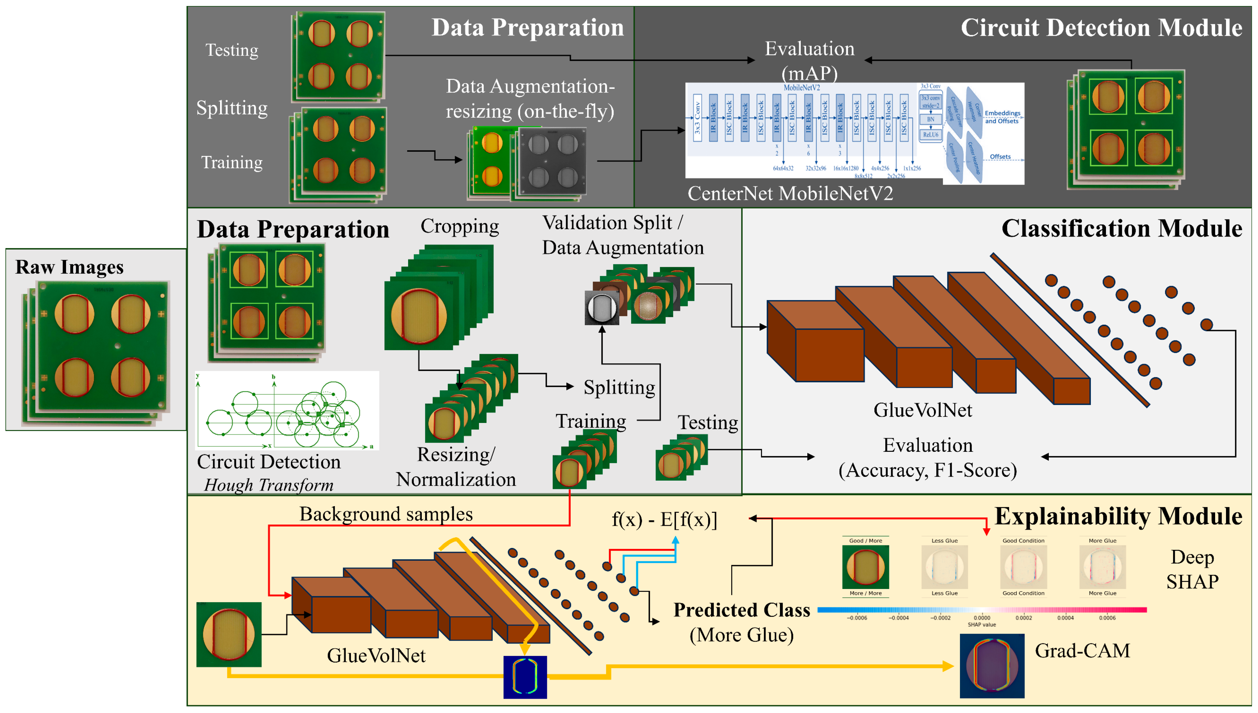
The overall proposed XAI framework for PCB glue inspection is presented in Figure 1 and consists of three modules. Initially, the raw data are passed to the Circuit Detection Module that aims to accurately localize all available circuits in a PCB board. Subsequently, the Classification Module classifies each detected circuit based on the placed glue volume. Finally, the XAI Module leverages the interpretability of the black-box classifier by providing the end users with insights into the model’s working principle. As it is comprehensively presented in Figure 2, each module in the framework is built and tested separately, and the specifics are delineated in the subsequent sections. The methodology is developed in the Python programming language (version 3.10) with the use of open packages such as TensorFlow 2.9.1 [51] for developing CNNs, OpenCV 4.10.0 [52] for image processing, and Matplotlib 3.7.1 [53] for data visualization.

3.1. Dataset

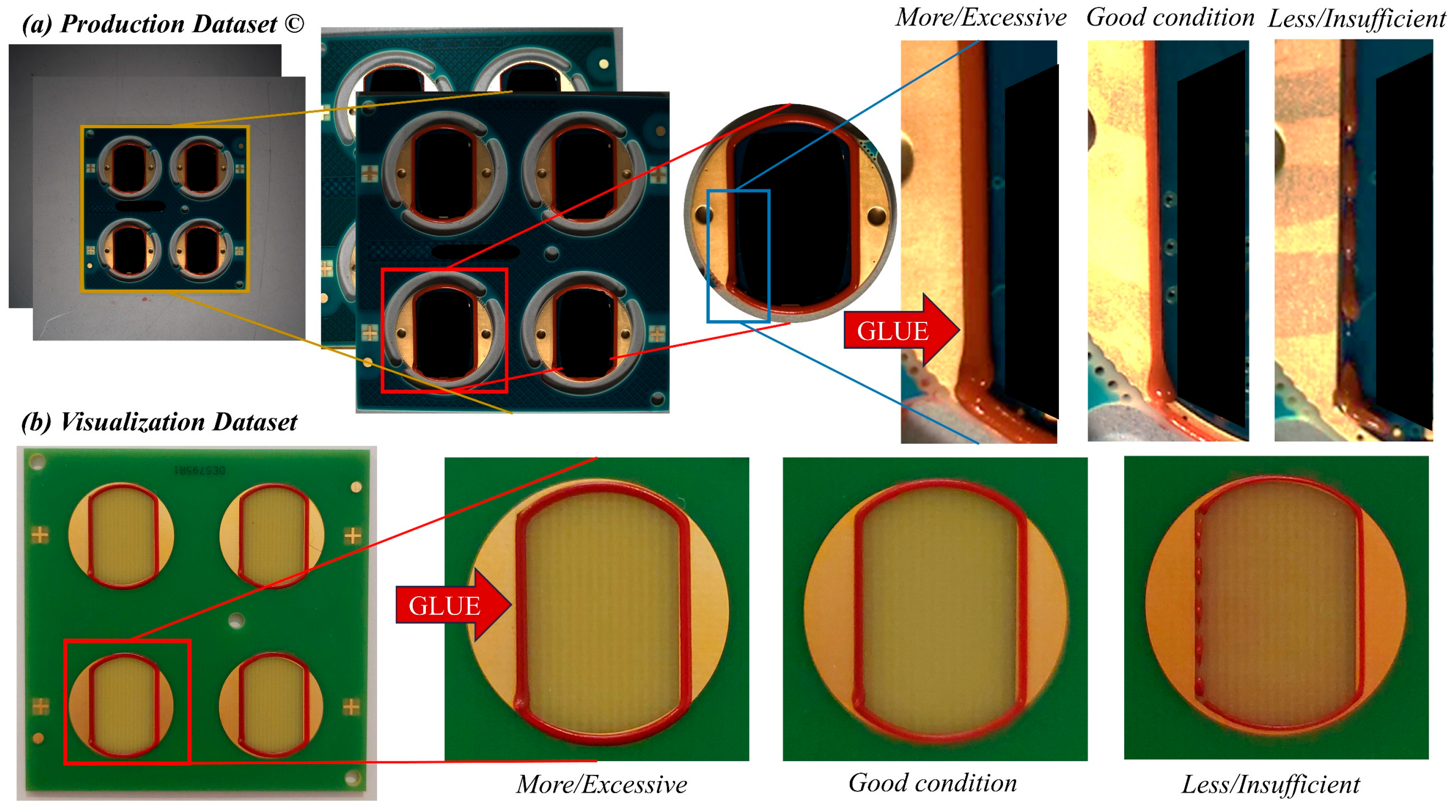
In real industrial environments, datasets are often limited, with defective classes particularly underrepresented [15,54]. This presents a significant challenge in developing robust data-driven tools. A similar situation was encountered in this study. To simulate real-world variability encountered during glue dispensing on production lines, a set of 100 printed circuit boards (PCBs) was meticulously fabricated by production personnel. These PCBs deliberately exhibited a wide range of potential glue dispensing outcomes, encompassing scenarios from insufficient to excessive glue application. Moreover, each PCB panel incorporated four identical printed circuits. This design ensured that the dispensing parameters were meticulously controlled, resulting in approximately the same glue quantity per circuit within a single panel. Consequently, the operators categorized each PCB board into three classes based on the glue volume condition: (1) less/insufficient glue for 24 PCBs, (2) good condition for 18 PCBs, and (3) more/excessive glue for 58 PCBs. It is worth mentioning that the creation and labeling of such a dataset required both production and human resources, which inherently limited the amount of data that could be generated.
To introduce a degree of quantification into the labeling process and reduce subjectivity, the glue dispensing procedure was systematically controlled through the adjustment of diffuser pressure, a parameter strongly correlated with glue volume. A golden sample was fabricated to establish the mean of the pressure distribution, representing the target standard for acceptable glue application. Samples with values close to this mean were considered to exhibit optimal glue volume, while deviations on either side corresponded to insufficient or excessive application. To formalize this categorization, a standard deviation of 1 (σ = 1) was used as the threshold for acceptable variance, with pressure values within this range labeled as “good”. However, these thresholds were used as practical guidelines rather than absolute limits, and their adjustment reflects the level of strictness applied in enforcing quality standards. It is important to note that the boundaries between classes are inherently fuzzy due to the gradual nature of glue volume variation. Consequently, samples near the class boundaries may exhibit ambiguous features, and misclassifications are more likely in these transitional regions. This reflects the physical variability of the dispensing process and mirrors the challenges typically encountered in real-world industrial settings.
The industrial area scan camera, the Baumer VCXG-201.R, was employed to capture a high-resolution RGB image from each PCB board. Notably, the image acquisition process was conducted under varying ambient lighting conditions, reflecting the potential variability encountered in real-world production environments. In addition, PCBs were not precisely centered in the frame, allowing for the inclusion of different viewing angles. In contrast, the focal distance is kept constant throughout the data acquisition process. This setup closely mimics a typical station on a production line, where PCBs are placed for automated visual quality inspection.
The images used for training and evaluating the model contained customer-specific PCB layouts, which must remain undisclosed. All samples consist of the same layout and the same glue pattern, with red glue being placed perimetrically of the circuits (Figure 3). To ensure privacy while demonstrating our approach, we generated a few additional PCB samples with the customer-specific layout removed. These modified samples are primarily used for visualization purposes in this paper. Figure 3 showcases a curated selection of samples from both datasets specifically chosen to illustrate the range of glue dispensing outcomes encountered. It is worth mentioning that the dataset encompasses a broader range of variability, and these images do not fully convey the uniqueness and complexity of the data.

3.2. Circuit Detection Module

As mentioned previously, each board is fabricated with four identical printed circuits. Their separation enhances the quality inspection procedure as it considers all available circuits and provides more specific data to the classifier. Moreover, the tiny sizes of the PCBs induce background noise even when they have a close distance from the image sensor, as presented in Figure 3 and the raw PCB image.
The core objective of the circuit detection module is to achieve rapid and accurate detection of all circuits present on the PCB board, while simultaneously minimizing the computational requirements. Initially, the standard machine vision algorithm, circle Hough transform [55], was implemented as an automatic cropping tool during the pre-processing stage. While this method successfully identified all circuits within the employed dataset, achieving 100% accuracy, it is crucial to acknowledge its limitations. This exceptional performance can be attributed in part to the controlled laboratory environment under which the image data was captured (uniform background, standardized focal distance, centered object placement, etc.). These ideal conditions simplify the task and may not reflect real-world scenarios with potentially higher noise levels or less stringent data acquisition procedures. Consequently, the generalizability of Hough transform in such scenarios may be compromised.
According to the research findings [50], DL models for OD and semantic segmentation are alternative methods for localizing circuits in PCBs. OD models are robust against translational, rotational, and scaling invariances of the objects of interest and do not employ parameters for the detection, such as Hough transform. However, such models may substantially increase the computation needs and the processing times. Hence, the lightweight CenterNet [21] with MobileNetV2 [20] backbone network is utilized to replace Hough transform in the circuit detection task. The model is developed with the TensorFlow Object Detection Python Library (TFOD) [56]. The bounding boxes (BB) of the PCB circuits are manually annotated in the PASCAL VOC [57] format. To alleviate data scarcity, a pre-trained on COCO dataset [58] model is fine-tuned for the circuit detection task. Moreover, heavy data augmentation is performed on-the-fly during training for regularization. The model is trained with the Adam optimizer [59], and a batch size of 16 is chosen based on the available system’s RAM. In Adam, a cosine learning rate decay function is employed for more robust learning, with 1 × 10⁻⁴ base, 5 × 10⁻⁵ warmup learning parameters, and a warm-up period of 2000 training steps. As in the original TFOD implementation of CenterNet MobileNetV2, the default L1 loss and focal loss [60] are employed for penalizing localization and classification respectively.
The standard COCO OD metric [58] of mean average precision (mAP) (1) across 10 incremental intersection over union (IoU) (2) thresholds {0.5 + 0.05 · tt ∈ {0, 1, …, 9}} is employed to assess the performance of the task.
m A P = 1 N 1 C t = 1 N i = 1 C A P i t
Here, ∣C∣ is the total number of classes with ∣C∣ = 1 herein, and A P i t is the average Precision (3) for class i at IoU threshold t calculated as the area under the curve of the Precision × Recall curve at various confidence thresholds. Precision (4) measures the fraction of correct detections among all detected instances, while Recall (5) measures the fraction of correct detections among all ground truth instances. Confidence is a value in [0, 1] that exhibits the level of certainty or probability assigned by the model to a particular detection as follows:
I o U = A r e a   o f   O v e r l a p A r e a   o f   U n i o n = P r e d i c t e d   B B G r o u n d   T r u t h   B B P r e d i c t e d   B B G r o u n d   T r u t h   B B
A P = 0 1 P r e c i s i o n R e c a l l d R e c a l l
P r e c i s i o n = T r u e   P o s i t i v e s T r u e   P o s i t i v e s + F a l s e   P o s i t i v e s
R e c a l l = T r u e   P o s i t i v e s T r u e   P o s i t i v e s + F a l s e   N e g a t i v e s

3.3. Classification Module

To automate the glue volume inspection, the most efficacious CNN classifier is investigated herein. Similar to the circuit detection module, this module aims to achieve the highest classification efficiency while maintaining optimal processing requirements. To begin with, a CNN model architecture that maximizes the classification metrics is pursued. During experiments, the ten-fold cross validation method is utilized for the assessment of various CNN models. This method provides a statistically rigorous estimation of model performance, as it ensures that each sample, including rare cases, contributes to both training and validation phases.
An extensive exploration process is conducted that involves different convolutional layers, number of filters, kernel sizes, depths, and residual connections to attain the best-performed model. In addition, training with random weight initialization, as well as transfer learning with state-of-the-art models, are employed to further examine the best strategy. Likewise the work of [36], the best-found model, named as GlueVolNet, consists of an undemanding architecture that is depicted in Figure 4. A deep network is constructed, embodying four sequential blocks of convolutional—pooling—dropout layers, two dense layers, ReLU activation function, followed by a final three-node output layer with the SoftMax activation function. The 250 × 250 image input dimension is proven to be adequate for this dataset. The initial convolutional layer includes 3 × 3 filters (kernels) with no padding and strides of 1 × 1, followed by a 2 × 2-sized max-pooling layer with 2 × 2 strides and a dropout layer entailing a dropout rate of 0.2. The first convolutional layer is formed by 16 filters, whereas in each consecutive layer, the number of filters is doubled. A flattening operation is then utilized to transform the tensors to one-dimension arrays so that they are inserted into the two-layer dense network which consists of 128 and 64 nodes, respectively.
Regarding training, the Adam optimizer is utilized [59] with the default parameters along with the early stopping callback and the categorical cross entropy function.
The proposed GlueVolNet is compared to other types of CNN architectures to prove its efficacy. In detail, a CNN with different branches named as Branch-ResNet, and the pre-trained VGG16, VGG19 [25], ResNet50 [28], and MobileNetV2 [20] are assessed for this task. All the examined models receive the same training parameters, activation functions (ReLU), number of dense layers, and dropout regularization parameters.
The Branch-ResNet CNN utilizes three branches of two-layer CNNs with different kernel sizes after the input layer to increase the receptive field and to capture different scales or aspects of the input, inheriting the aspects of the inception module [29]. These branches are then added together in a residual block. Finally, the widely adopted pre-trained VGG16, VGG19, ResNet50, and MobileNetV2 are utilized with transfer learning. The choice for comparative models is deliberate and justified by their established performance and widespread adoption in image processing tasks across diverse domains [61]. These architectures are not only well-documented and supported but also computationally efficient, especially when applied to mid-scale industrial tasks [62]. These models remain benchmarks in the field, and their use ensures comparability and reliability when assessing the performance of novel approaches. The pre-trained models are trained in two stages as the literature suggests [63]. Initially, only the dense layers are trained with the standard learning rate of the Adam optimizer. Subsequently, all layers, except for the batch-normalization, are fine-tuned with a small learning rate of 0.00001.
To assess performance, the Precision (4), Recall (5), Accuracy (6), and F1-Score (7) metrics are used:
A c c u r a c y = T r u e   P o s i t i v e s + T r u e   N e g a t i v e s T o t a l   P o p u l a t i o n
F 1 - Score = 2 × P r e c i s i o n × R e c a l l P r e c i s i o n + R e c a l l

3.4. XAI Module

The explainability of the classification scheme was further investigated, and two different post-hoc XAI approaches were examined, namely, Deep SHAP [10] and Grad-CAM [19].
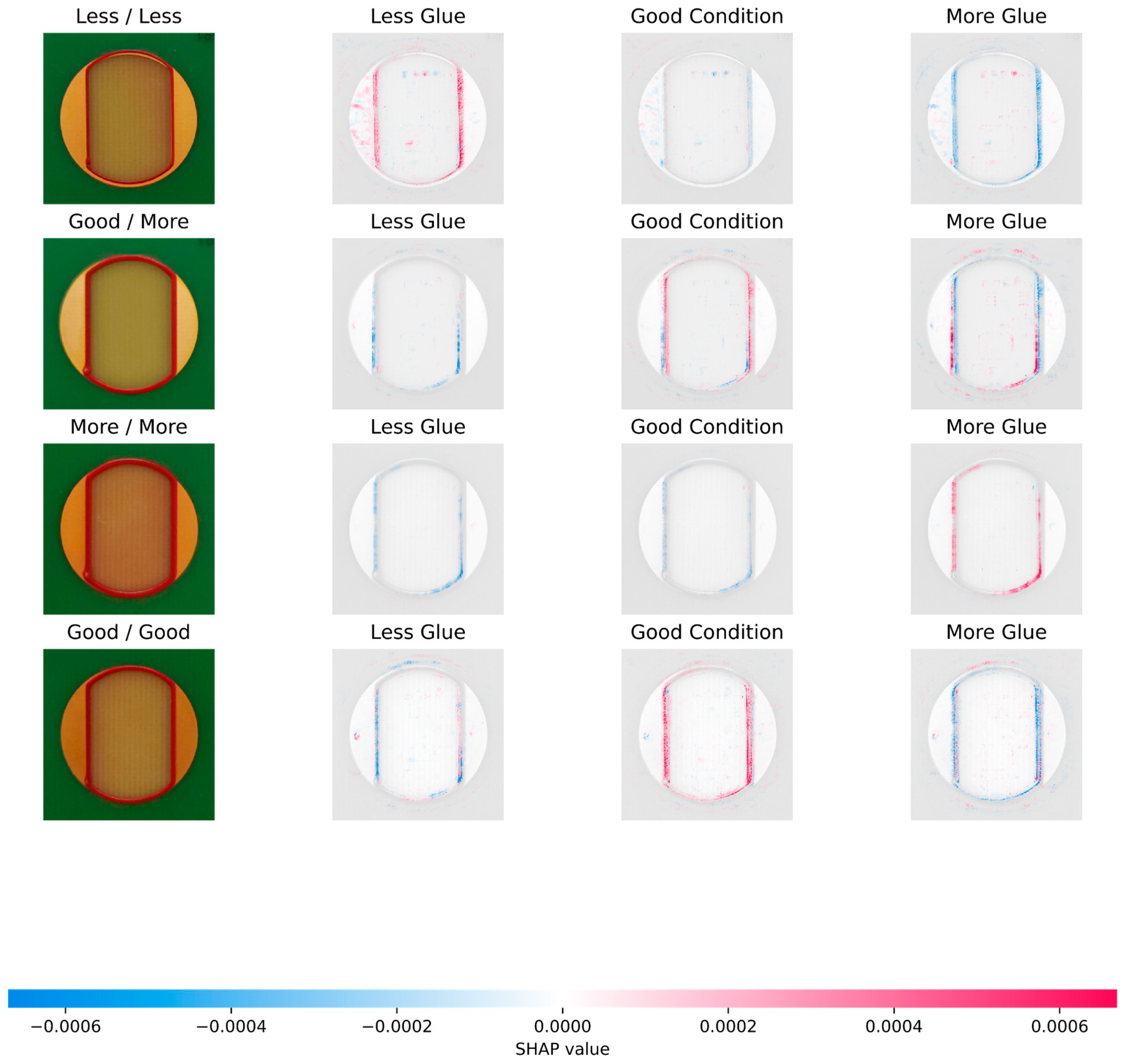
On one hand, Deep SHAP is utilized from the Python SHAP package. Regarding the background samples, 100 arbitrary images from the training dataset are utilized for integrating out features, following the official package recommendation regarding the best trade-off between accuracy and processing speed. Deep SHAP uses this background dataset to calculate the expected output of the trained model. The output of Deep SHAP for a new testing sample is the SHAP value, or the score, of each pixel area to the decision of CNNs. A diverging blue-red colormap is employed to visualize the scores, where blue indicates a pixel area with a negative influence toward a class, while red means a positive influence.
On the other hand, the output of Grad-CAM is a heatmap visualization for a given class label that highlights the important regions in the image for predicting that label. In detail, the weights of the feature maps of the last convolutional layer are calculated and a global average pooling is applied. By calculating the weighted sum of the pooled values and by filtering zero values the heatmap is generated. This heatmap can be resized to the input image dimension and can be placed on top of the image to ensure interpretability.

3.5. Data Preparation

3.5.1. Cropping

This step is essential to generate a proper dataset for the classification models. A circle Hough transform [55] is initially employed to detect circle shapes in the raw images. A median filter is applied in the raw images to eliminate noise and preserve edges. The Hough gradient method in the Hough circles function of the OpenCV python package [52] is utilized by providing the following parameters: dp = 2, minimum distance = 500, p1 = 30, p2 = 500, minimum radius = 50, and maximum radius 500. The average size of the cropped images is 840 × 840 pixels. To ensure that no useful glue information was lost during cropping, a margin was maintained around the detected circle.

3.5.2. Resizing and Normalization

The 840 × 840-pixel size derived after cropping still adds a lot of unnecessary computation in the developed models. Therefore, the images are resized prior to training to a 250 × 250-pixel size with the use of the widely adopted bilinear interpolation method. Regarding the OD scheme, the resizing to the 512 × 512-pixel size requirement of CenterNet MobileNetV2 is performed on-the-fly with the same method. Finally, all image pixel values are normalized to [0, 1].

3.5.3. Splitting

The splitting into training and testing is performed automatically with the use of the K-fold method of the scikit-learn [64] python package. Utilizing a ten-fold scheme, 10% of the dataset is randomly kept for testing. For the remaining training dataset, 20% is kept for validation to monitor training.

3.5.4. Data Augmentation

Geometrical data augmentation (DA) techniques are applied to artificially increase the training dataset. For the classification, ImageDataGenerator from the Keras python library is utilized to generate batches of tensor image data with on-the-fly DA. In detail, the DA that is utilized involves random variations in shear transformation, zooming, horizontal/vertical flipping, rotation, and shifting.
In addition, the cropping with a sliding window is also examined as the DA technique. By resizing the images in a size slightly larger than the input dimension of the model (e.g., to 350 × 350-pixel size), we can extract several image patches of 250 × 250-pixel size from the original image. In detail, by starting from the upper left corner of the image, and by controlling the strides (steps) in x,y axes in which the 250 × 250 cropping area slides, we can generate more cropped images from the raw image. Moreover, by providing smaller strides for the classes with minority samples, we can artificially mitigate the data imbalance. A stride of 11 pixels in both axes is selected for the “good condition” class, whereas a stride of 13 pixels is utilized for the rest classes. Hence, 100 cropped images are generated for each image in the minority class and 64 cropped images for each image in the majority classes.
Regarding the OD task, the employed DA techniques involve both geometrical and color transformations, as well as noise insertion, to ensure the generalization of the model even in noisy data.

4. Results and Discussion

The experimental procedures are conducted using a personal computer (PC) with the following specifications: an Intel Core i9 processor clocked at 3.5 GHz, 16 GB of DDR4 RAM, and an NVIDIA GeForce RTX 3080 graphics card. The operating system utilized is Windows 10 Professional.

4.1. Circuit Detection

Following the proposed XAI framework for glue dispensing, the Circuit Detection Module is initially examined. Two approaches are investigated, the traditional circle Hough transform (CHT) method and the CenterNet MobileNetV2 CNN model, which both achieve high accuracy. The comparative results for the printed circuit detection are summarized in Table 1. The model is trained for 8000 steps. The achieved 100% mAP at 0.75 IoU of CenterNet MobileNetV2 indicates the ability to detect all circuits with high overlap between the ground truth and the predicted bounding box.
In addition to accuracy, the deep model proved to be more computationally efficient than the CHT. Notably, the CenterNet MobileNetV2 model does not require manual parameter tuning, such as the specification of minimum and maximum radius values, which in CHT are sensitive to factors like focal length and scaling. This highlights the flexibility and robustness of deep OD methods in variable imaging conditions.
Moreover, the inclusion of the CHT serves as a baseline comparison to traditional, non-ANN machine vision techniques, which rely on filters and edge detection algorithms to identify geometric patterns such as circles. While deep learning is increasingly favored across computer vision domains due to its performance and adaptability [65], traditional methods have been extensively used in similar industrial tasks, as noted in Section 2.2 and supported by prior works [45,46,47]. However, the empirical results of this study clearly demonstrate that the DL-based method outperforms the traditional approach. This is particularly significant given the small size of the training dataset, a scenario in which DL models often struggle. In contrast, CenterNet MobileNetV2 maintained high performance, confirming its suitability and advantage for deployment in real-world production environments where robust, fast, and adaptive solutions are essential.

4.2. Classification

Concerning the classification task, various state-of-the-art CNN models are examined and deployed to the image dataset. A comparative analysis among the efficient CNN models is conducted and the results are gathered in Table 2. In particular, it presents the attained classification metrics for each examined CNN model, using ten-fold cross validation.
In cross-validation, the training and validation sets, as these defined in Section 3.5.3, are used by the early stopping algorithm, which terminates training if the validation loss does not improve after 20 consecutive epochs and restores the model weights corresponding to the lowest validation error. By setting a relatively high maximum number of epochs and incorporating early stopping with high patience, each model is allowed to train efficiently while minimizing the risk of underfitting or overfitting, at the cost of a prolonged training.
From the examined models, the proposed GlueVolNet architecture is the most efficient, providing both high accuracy and F1-score. The worst performance is attained by MobileNetV2, which fails to increase its classification ability even when the whole network is fine-tuned in the PCBs dataset. The Branch-ResNet CNNs also present pure metrics. On the contrary, the other pre-trained models such as VGG16, VGG19, and ResNet50 are able to produce high classification metrics in the second training stage of the fine-tuning. In fact, VGG19 proves to be the second most efficient model from the experimentation process. To sum up, GlueVolNet proves to be the most accurate model for this task. The attained accuracy is 2% higher than the second-best attained accuracy of VGG19. Moreover, both the classification report and the confusion matrix of an average run for GlueVolNet, as presented in Table 3 and Table 4, respectively, indicate difficulties in capturing the “good condition” minority class.
Regarding processing times, the simple architecture of GlueVolNet requires approximately 55 milliseconds and 95 milliseconds to perform batched inference in GPU and CPU, respectively, using a batch size of four, which is the same as the number of circuits in each board. The reported times indicate that the proposed approach requires significantly less processing time than the traditional CHT method, further proving the efficiency of the proposed approach compared to traditional methods. In addition, CNNs alleviate the need for the extensive handcrafted pre-processing, threshold tuning, and regular retraining to maintain performance involved with traditional approaches [45,46,47]. GlueVolNet learns hierarchical feature representations directly from data, enabling end-to-end classification from raw images with minimal manual intervention and with robust accuracy. Although a direct comparison with traditional approaches would more clearly reveal the strengths and weaknesses of the DL method, preliminary assessments indicated that conventional techniques were sensitive to the gradual and subtle variations in glue volume.
The sliding window augmentation method is employed to examine the classification performance in a bigger and to some extent more balanced dataset. GlueVolNet achieves 0.901 ± 0.032 accuracy and a 0.898 ± 0.029 F1-Score, which indicates a slight improvement (1%) in the generalization of the model across all classes, as also presented in the classification report (Table 5) and the confusion matrix (Table 6).
Moreover, the misclassifications of the sliding window experiments, which essentially are cropped parts of the original images, indicate that either there is an uneven distribution of glue in the printed circuit, or some glue areas contribute more to the final decision. Grad-CAM and Deep SHAP visualizations could reveal the spatial areas the CNN focuses on during prediction to further investigate model’s decision-making.
Finally, it is worth noting that the fixed glue color and pattern may have benefited the model’s classification accuracy. This presents a potential limitation in the model’s generalizability to different glue patterns, which requires further investigation in future work. A preliminary assessment using heavily processed images to distort color in the current dataset showed a noticeable drop in accuracy. Although GlueVolNet could partially address this limitation through color transformations during data augmentation, which was not applied in this study, evaluating the model using real-world color variations would provide more robust insights.

4.3. XAI Visualizations

Being a black-box model, GlueVolNet cannot provide insights into the decision making. This can be mitigated with the explainable DL methods of Grad-CAM and Deep SHAP. These methods are applied to the GlueVolNet model of the original dataset (no sliding-window), acting on the whole images, in order to clarify and uncover the decision making.
Initially, the Grad-CAM method is applied, and some representative results are presented in Figure 5. In particular, one original testing image is depicted for each category followed by the heatmaps generated using the Grad-CAM method, and the visualization result is generated by superimposing the original image on the heatmap. Different colors indicate the importance of pixels in the classification results, representing the sensitivity of the CNN classifier to each pixel. Regarding the first example with the “Less glue” class, the area that forced the model to this decision is on the left of the circuit where strong red values are observed. The absence of glue in that location verifies the decision. Grad-CAM indicates that the bottom left corner deposit, which is the point where dispensing begins, is utilized by the model to predict the “good condition” class. This exposes a potential reason for the misclassification of the “good condition” class when this area has uneven glue deposits. Regarding “more glue”, Grad-CAM exposes almost the whole glue region as the model’s decision, with the most intense values being noticeable in the two vertical lines.
To further analyze the model’s behavior, the SHAP values in Figure 6 are elaborately studied. Each row in the figure depicts a testing sample. Positive SHAP values (red color) indicate the pixel areas that contributed to this class, and vice versa. These values are clearly noticeable in the correctly identified instances of rows 1, 3, and 4. However, by examining the image on the second row, which was misclassified as “more glue”, we can uncover the glue pixel areas that forced the model to this decision. Moreover, an uneven glue deposit is noticeable in the vertical glue lines, as high SHAP values in the “more glue” class are present. Such an interpretable result is beneficial to understanding the decision-making and contributes to process optimization, as it can reveal uneven glue dispensing.
It is also concluded based on the experiments, that both Deep SHAP and Grad-CAM employ similar glue areas for the decision interpretation, by examining the testing dataset. Such uneven glue deposits indicate that traditional methods that typically rely on fixed thresholds would struggle to correctly identify classes. Comparing the employed post-hoc XAI methods, it is observed that Deep SHAP offers more comprehensive explanations as it differentiates the significant pixel areas between classes. Furthermore, the quality of the explanations is validated by utilizing operators’ feedback, which confirms that the highlighted areas indicated by the post-hoc methods are indeed helpful for decision making.
Deep SHAP requires approximately 5 and 37 s for GPU and CPU processing, respectively, to provide explanations about four printed circuits and by employing a background sample of 100 images. Compared to the time needed for the Grad-CAM computation, which matches the model’s inference speeds, it is observed that Deep SHAP might be inappropriate for industrial cases with limited hardware resources or when real-time processing is crucial.
The application of Grad-CAM and Deep SHAP to the GlueVolNet model highlights complementary strengths and limitations, making them suitable for different production scenarios. Grad-CAM is computationally efficient and integrates seamlessly into real-time processes, making it an ideal choice for applications where speed is critical, such as in high-throughput manufacturing lines. Its heatmaps offer intuitive visual explanations, but they may lack the detailed differentiation of influential regions provided by Deep SHAP. On the other hand, Deep SHAP excels in offering a more granular and class-specific understanding of the model’s decision-making process. This makes it highly beneficial for diagnostic purposes, process optimization, and scenarios where understanding subtle variations in glue deposition is crucial. However, its higher computational cost may limit its application in real-time or resource-constrained environments.
Depending on production needs, these methods can be used individually or in combination. Grad-CAM can serve as a rapid, first-line tool for routine quality checks, while Deep SHAP can be deployed for in-depth analysis in cases of recurring misclassifications or process deviations. By combining these tools, manufacturers can balance efficiency and explainability, leveraging Grad-CAM for real-time decision support and Deep SHAP for detailed diagnostics and process refinement.
Finally, it is important to note that post-hoc visualizations illustrate that the model relies on visual cues correlated with volume, such as spread area and edges, to infer apparent glue volume from a single top-down 2D RGB image. Since volume is a 3D property, the proposed approach may not accurately distinguish between variations in glue height. Although the work of [50] concluded that a 2D soft sensor is applicable, future work should investigate integrating depth-sensing or multi-view imaging to provide more physically grounded volume assessments.

4.4. Time Efficiency and Edge Processing

This section highlights the reported processing times to identify potential bottlenecks that may affect real-time performance. In industrial applications, real-time processing typically refers to inference latencies that are equal to or less than the latency of the corresponding production task, thereby ensuring no additional delays between sequential manufacturing steps. Although the actual glue dispensing process lasts several seconds, and without disclosing proprietary information, real-time operation in this context is defined as achieving at least 0.5 frames per second (FPS). To assess the inference performance of the proposed method, evaluations were conducted not only on a high-performance desktop machine but also on a low-cost edge device, namely, the NVIDIA Jetson Nano. The Jetson Nano features an NVIDIA Maxwell GPU architecture, a quad-core ARM Cortex-A57 MPCore CPU, and 4 GB of LPDDR4 shared memory between the CPU and GPU. Python 3.6 is used alongside ARM-optimized versions of TensorFlow and OpenCV.
An end-to-end assessment was performed using a dataset of 50 samples. Each image was first processed using the CenterNet MobileNetV2 model to detect and isolate individual circuits. The four cropped regions per image were then resized and passed through the GlueVolNet classifier in a single batch inference using Keras. After classification, each cropped region was reprocessed through GlueVolNet to generate Grad-CAM heatmaps. Heatmap generation and storage were performed using Matplotlib at a resolution of 300 dots per inch (dpi). Class predictions and Grad-CAM visualizations were evaluated separately to simulate scenarios where visual explanations are not required. Deep-SHAP visualizations were excluded due to their known high computational overhead. The reported results are averaged over all test samples and summarized in Table 7. For the Jetson Nano, only CPU processing times are reported, as loading both models on the GPU resulted in memory allocation failures. These failures stem from the device’s limited shared memory between the operating system, graphical user interface, and GPU, revealing a practical limitation in deploying large models concurrently. To ensure reliable timing, the initial model inference was performed on a dummy image (excluded from results), mitigating the latency introduced by TensorFlow’s initial graph construction and CUDA kernel warm-up.
From an algorithmic perspective, the proposed framework achieves real-time performance on high-end desktop systems, with both CPU and GPU implementations exceeding 4 FPS. The primary processing bottleneck is attributed to Grad-CAM heatmap rendering, which is not GPU-accelerated due to limitations in the Matplotlib backend. As a result, the pipeline operates near real-time at approximately 0.5 FPS, which is sufficient to keep pace with the manufacturing process. Given that each PCB requires more than two seconds for glue dispensing, the automated inspection does not impede production throughput. Conversely, the Jetson Nano implementation does not meet the defined real-time criteria. The elevated latency is primarily due to CPU-only inference and limited memory bandwidth, further compounded by non-accelerated heatmap rendering.
To address these limitations, future work may explore GPU-accelerated visualization libraries to replace Matplotlib, reducing latency for both desktop and embedded systems. Additionally, converting the framework into an edge-optimized pipeline, leveraging lightweight models and inference engines such as TensorRT or TensorFlow Lite, could enable practical deployment even on low-end GPU-equipped devices.

5. Summary

This research presents a novel explainable artificial intelligence (XAI) quality inspection framework for detecting inconsistencies in glue volume applied to printed circuit boards (PCBs). The primary contribution of this study lies in integrating advanced machine vision techniques with explainability methods to enhance accuracy, efficiency, and trustworthiness in PCB quality assurance processes. This framework is specifically tailored to automate and streamline quality inspection in a real-world industrial setting within the electronics sector.
The proposed system commences with the deployment of a lightweight CenterNet MobileNetV2 object detector. This detector is specifically chosen due to its ability to rapidly and precisely localize individual PCBs within the image. Following successful localization, a custom convolutional neural network (CNN) classifier, named GlueVolNet, categorizes PCBs based on the volume of the glue dispensed. The proposed GlueVolNet architecture is then compared head-to-head with other industry-leading CNN classifiers to validate performance. GlueVolNet demonstrates its efficacy by achieving classification accuracy of 92.2%, while simultaneously maintaining rapid inference speeds owing to its streamlined architecture.
The developed tool focuses exclusively on CNNs; therefore, only a limited performance comparison is made against traditional machine vision approaches that remain applicable to similar tasks. While this may be seen as a potential limitation in terms of exploring simpler alternatives, the results indicate that the common drawbacks of CNNs, such as the need for large datasets or complex tuning, have been effectively addressed. Moreover, the circle Hough transform, used as a baseline method for circuit detection, was found to be time inefficient in comparison. In contrast, CNNs offer the significant advantage of automatic feature extraction and selection, enabling a more flexible and scalable solution that requires minimal manual intervention.
Furthermore, to address the need for interpretability, another drawback of CNNs, the framework integrates Deep SHAP and Grad-CAM explainability methods. These methods highlight the pixel regions contributing most significantly to classification decisions. Grad-CAM and Deep SHAP offer complementary strengths, with Grad-CAM excelling in real-time efficiency for high-throughput applications and Deep SHAP providing detailed, class-specific insights ideal for diagnostics and process optimization. These visualizations empower operators to readily identify and comprehend uneven glue deposits on PCBs, bridging the gap between automated systems and human expertise.
The findings demonstrate the potential of the proposed machine vision methods to significantly enhance production efficiency and product quality by automating glue volume inspection and providing accurate, interpretable outputs. However, the current reliance on supervised learning and specific datasets introduces limitations in generalizability. Currently, a case-specific and limited dataset could be assembled to include sufficient images of faulty PCBs for effectively training deep models as the effort of collecting and labelling data temporarily diverted production resources and introduced additional overhead, making it a non-trivial and costly task.
This limitation hinders the proposed scheme’s ability to generalize to other types of PCBs and varying dispensing processes. Future work will prioritize acquiring a more diverse dataset to cover a broader range of glue dispensing scenarios, with even broader lighting conditions and angles, thus enabling the system to adapt to diverse manufacturing environments and assessing its generalization capabilities. Furthermore, experimentation with a larger dataset would facilitate the exploration of a wider range of models, including the latest advancements in Vision Transformers, addressing another potential limitation of this work. Finally, generalization assessment should also consider the limitations of using 2D representations to infer glue volume, which is inherently a 3D property.

Author Contributions

Conceptualization, T.T. (Theodoros Tziolas), K.P. and E.P.; methodology, T.T. (Theodoros Tziolas); software, T.T. (Theodoros Tziolas); validation, K.P., T.T. (Theodosios Theodosiou), N.D., G.T. and E.P.; formal analysis, T.T. (Theodoros Tziolas); investigation, T.T. (Theodoros Tziolas); resources, D.I., N.D. and E.P.; data curation, D.I., G.T. and N.D.; writing—original draft preparation, T.T. (Theodoros Tziolas); writing—review and editing, K.P., T.T. (Theodosios Theodosiou) and E.P.; visualization, T.T. (Theodoros Tziolas) and K.P.; supervision, T.T. (Theodosios Theodosiou) and E.P.; project administration, E.P.; funding acquisition, N.D. and E.P. All authors have read and agreed to the published version of the manuscript.

Funding

This work has been supported by EU Project OPTIMAI (H2020-NMBP-TR-IND-2020-singlestage, Topic: DT-FOF-11-2020, GA 958264).

Data Availability Statement

The datasets used in this study, both original and anonymized versions for visualization, are owned by the OPTIMAI research consortium. The original dataset contains proprietary and confidential customer-designed components and cannot be made publicly available. The anonymized dataset used for visualization, which excludes customer-specific layouts, is part of an ongoing study and is not currently available for public release. Requests to access the anonymized dataset may be directed to Dr. Nikolaos Dimitriou.

Conflicts of Interest

One of the authors is affiliated with Microchip Technology, Inc., which provided the image data. This relationship is disclosed in the interest of transparency. The authors declare that this affiliation did not influence the research findings.

References

  1. Gryna, F.M.; Juran, J.M. Quality and Costs; McGraw-Hill: New York, NY, USA, 1999. [Google Scholar]
  2. Ebayyeh, A.A.R.M.A.; Mousavi, A. A Review and Analysis of Automatic Optical Inspection and Quality Monitoring Methods in Electronics Industry. IEEE Access 2020, 8, 183192–183271. [Google Scholar] [CrossRef]
  3. Wang, M.-J.J.; Huang, C.-L. Evaluating the Eye Fatigue Problem in Wafer Inspection. IEEE Trans. Semicond. Manuf. 2004, 17, 444–447. [Google Scholar] [CrossRef]
  4. Ali, S.; Abuhmed, T.; El-Sappagh, S.; Muhammad, K.; Alonso-Moral, J.M.; Confalonieri, R.; Guidotti, R.; Ser, J.D.; Díaz-Rodríguez, N.; Herrera, F. Explainable Artificial Intelligence (XAI): What We Know and What Is Left to Attain Trustworthy Artificial Intelligence. Inf. Fusion 2023, 99, 101805. [Google Scholar] [CrossRef]
  5. Nguyen Ngoc, H.; Lasa, G.; Iriarte, I. Human-Centred Design in Industry 4.0: Case Study Review and Opportunities for Future Research. J. Intell. Manuf. 2022, 33, 35–76. [Google Scholar] [CrossRef]
  6. Arrieta, A.B.; Díaz-Rodríguez, N.; Ser, J.D.; Bennetot, A.; Tabik, S.; Barbado, A.; Garcia, S.; Gil-Lopez, S.; Molina, D.; Benjamins, R.; et al. Explainable Artificial Intelligence (XAI): Concepts, Taxonomies, Opportunities and Challenges toward Responsible AI. Inf. Fusion 2020, 58, 82–115. [Google Scholar] [CrossRef]
  7. Sagi, O.; Rokach, L. Approximating XGBoost with an Interpretable Decision Tree. Inf. Sci. 2021, 572, 522–542. [Google Scholar] [CrossRef]
  8. van der Waa, J.; Nieuwburg, E.; Cremers, A.; Neerincx, M. Evaluating XAI: A Comparison of Rule-Based and Example-Based Explanations. Artif. Intell. 2021, 291, 103404. [Google Scholar] [CrossRef]
  9. Vale, D.; El-Sharif, A.; Ali, M. Explainable Artificial Intelligence (XAI) Post-Hoc Explainability Methods: Risks and Limitations in Non-Discrimination Law. AI Ethics 2022, 2, 815–826. [Google Scholar] [CrossRef]
  10. Lundberg, S.; Lee, S.-I. A Unified Approach to Interpreting Model Predictions. In Proceedings of the Advances in Neural Information Processing Systems 30: Annual Conference on Neural Information Processing Systems 2017, Long Beach, CA, USA, 4–9 December 2017. [Google Scholar]
  11. Ribeiro, M.T.; Singh, S.; Guestrin, C. “Why Should I Trust You?”: Explaining the Predictions of Any Classifier. In Proceedings of the 22nd ACM SIGKDD International Conference on Knowledge Discovery and Data Mining, Association for Computing Machinery. San Francisco, CA, USA, 13–17 August 2016; pp. 1135–1144. [Google Scholar]
  12. LeCun, Y.; Bengio, Y.; Hinton, G. Deep Learning. Nature 2015, 521, 436–444. [Google Scholar] [CrossRef] [PubMed]
  13. Tercan, H.; Meisen, T. Machine Learning and Deep Learning Based Predictive Quality in Manufacturing: A Systematic Review. J. Intell. Manuf. 2022, 33, 1879–1905. [Google Scholar] [CrossRef]
  14. Zhou, Y.; Yuan, M.; Zhang, J.; Ding, G.; Qin, S. Review of Vision-Based Defect Detection Research and Its Perspectives for Printed Circuit Board. J. Manuf. Syst. 2023, 70, 557–578. [Google Scholar] [CrossRef]
  15. Tziolas, T.; Theodosiou, T.; Papageorgiou, K.; Rapti, A.; Dimitriou, N.; Tzovaras, D.; Papageorgiou, E. Wafer Map Defect Pattern Recognition Using Imbalanced Datasets. In Proceedings of the 2022 13th International Conference on Information, Intelligence, Systems & Applications (IISA), Corfu, Greece, 18–20 July 2022; pp. 1–8. [Google Scholar]
  16. Gu, J.; Wang, Z.; Kuen, J.; Ma, L.; Shahroudy, A.; Shuai, B.; Liu, T.; Wang, X.; Wang, G.; Cai, J.; et al. Recent Advances in Convolutional Neural Networks. Pattern Recognit. 2018, 77, 354–377. [Google Scholar] [CrossRef]
  17. Ibrahim, R.; Shafiq, M.O. Explainable Convolutional Neural Networks: A Taxonomy, Review, and Future Directions. ACM Comput. Surv. 2023, 55, 206. [Google Scholar] [CrossRef]
  18. Xie, D.; Wu, Z.; Hai, J.; Economou, M. Reliability Enhancement of Automotive Electronic Modules Using Various Glues. In Proceedings of the 2018 IEEE 68th Electronic Components and Technology Conference (ECTC), San Diego, CA, USA, 29 May–1 June 2018; pp. 172–178. [Google Scholar]
  19. Selvaraju, R.R.; Cogswell, M.; Das, A.; Vedantam, R.; Parikh, D.; Batra, D. Grad-CAM: Visual Explanations from Deep Networks via Gradient-Based Localization. Int. J. Comput. Vis. 2019, 128, 336–359. [Google Scholar] [CrossRef]
  20. Sandler, M.; Howard, A.; Zhu, M.; Zhmoginov, A.; Chen, L.-C. MobileNetV2: Inverted Residuals and Linear Bottlenecks. In Proceedings of the IEEE Conference on Computer Vision and Pattern Recognition (CVPR), Salt Lake City, UT, USA, 18–22 June 2018. [Google Scholar] [CrossRef]
  21. Zhou, X.; Wang, D.; Krähenbühl, P. Objects as Points. arXiv 2019, arXiv:1904.07850. [Google Scholar]
  22. Chen, L.; Li, S.; Bai, Q.; Yang, J.; Jiang, S.; Miao, Y. Review of Image Classification Algorithms Based on Convolutional Neural Networks. Remote Sens. 2021, 13, 4712. [Google Scholar] [CrossRef]
  23. Liu, Y.; Zhang, Y.; Wang, Y.; Hou, F.; Yuan, J.; Tian, J.; Zhang, Y.; Shi, Z.; Fan, J.; He, Z. A Survey of Visual Transformers. IEEE Trans. Neural Netw. Learn. Syst. 2024, 35, 7478–7498. [Google Scholar] [CrossRef] [PubMed]
  24. Maurício, J.; Domingues, I.; Bernardino, J. Comparing Vision Transformers and Convolutional Neural Networks for Image Classification: A Literature Review. Appl. Sci. 2023, 13, 5521. [Google Scholar] [CrossRef]
  25. Simonyan, K.; Zisserman, A. Very Deep Convolutional Networks for Large-Scale Image Recognition. In Proceedings of the 3rd International Conference on Learning Representations (ICLR 2015), San Diego, CA, USA, 7–9 May 2015; Computational and Biological Learning Society. pp. 1–14. [Google Scholar]
  26. Özdem, S.; Orak, İ.M. A Novel Method Based on Deep Learning Algorithms for Material Deformation Rate Detection. J. Intell. Manuf. 2024. [Google Scholar] [CrossRef]
  27. Ross, N.S.; Sheeba, P.T.; Shibi, C.S.; Gupta, M.K.; Korkmaz, M.E.; Sharma, V.S. A Novel Approach of Tool Condition Monitoring in Sustainable Machining of Ni Alloy with Transfer Learning Models. J. Intell. Manuf. 2024, 35, 757–775. [Google Scholar] [CrossRef]
  28. He, K.; Zhang, X.; Ren, S.; Sun, J. Deep Residual Learning for Image Recognition. In Proceedings of the IEEE Conference on Computer Vision and Pattern Recognition, Las Vegas, NV, USA, 27–30 June 2016; pp. 770–778. [Google Scholar]
  29. Szegedy, C.; Vanhoucke, V.; Ioffe, S.; Shlens, J.; Wojna, Z. Rethinking the Inception Architecture for Computer Vision. In Proceedings of the 2016 IEEE Conference on Computer Vision and Pattern Recognition (CVPR), Las Vegas, NV, USA, 27–30 June 2016; IEEE Computer Society: Los Alamitos, CA, USA, 2016; pp. 2818–2826. [Google Scholar]
  30. Howard, A.G.; Zhu, M.; Chen, B.; Kalenichenko, D.; Wang, W.; Weyand, T.; Andreetto, M.; Adam, H. MobileNets: Efficient Convolutional Neural Networks for Mobile Vision Applications. arXiv 2017, arXiv:1704.04861. [Google Scholar] [CrossRef]
  31. Ahmad, H.M.; Rahimi, A. Deep Learning Methods for Object Detection in Smart Manufacturing: A Survey. J. Manuf. Syst. 2022, 64, 181–196. [Google Scholar] [CrossRef]
  32. Tan, M.; Pang, R.; Le, Q.V. EfficientDet: Scalable and Efficient Object Detection. In Proceedings of the IEEE/CVF Conference on Computer Vision and Pattern Recognition (CVPR), Seattle, WA, USA, 13–19 June 2020. [Google Scholar]
  33. He, K.; Gkioxari, G.; Dollár, P.; Girshick, R. Mask R-CNN. In Proceedings of the 2017 IEEE International Conference on Computer Vision (ICCV), Venice, Italy, 22–29 October 2017; pp. 2980–2988. [Google Scholar]
  34. Theodosiou, T.; Tziolas, T.; Papageorgiou, K.; Rapti, A.; Papageorgiou, E.; Pantoja, S.; Charalampous, P.; Dimitriou, N.; Tzovaras, D.; Cuiñas, A.; et al. Centernet-Based Models for the Detection of Defects in an Industrial Antenna Assembly Process. In Proceedings of the 10th ECCOMAS Thematic Conference on Smart Structures and Materials, Patras, Greece, 3–5 July 2023; Department of Mechanical Engineering & Aeronautics University of Patras: Patras, Greece, 2023; pp. 1209–1220. [Google Scholar]
  35. Zhou, B.; Khosla, A.; Lapedriza, A.; Oliva, A.; Torralba, A. Learning Deep Features for Discriminative Localization. In Proceedings of the 2016 IEEE Conference on Computer Vision and Pattern Recognition (CVPR), Las Vegas, NV, USA, 27–30 June 2016; pp. 2921–2929. [Google Scholar]
  36. Papandrianos, N.I.; Feleki, A.; Moustakidis, S.; Papageorgiou, E.I.; Apostolopoulos, I.D.; Apostolopoulos, D.J. An Explainable Classification Method of SPECT Myocardial Perfusion Images in Nuclear Cardiology Using Deep Learning and Grad-CAM. Appl. Sci. 2022, 12, 7592. [Google Scholar] [CrossRef]
  37. Noh, E.; Hong, S. Automatic Screening of Bolts with Anti-Loosening Coating Using Grad-CAM and Transfer Learning with Deep Convolutional Neural Networks. Appl. Sci. 2022, 12, 2029. [Google Scholar] [CrossRef]
  38. Hacıefendioğlu, K.; Adanur, S.; Demir, G. Automatic Landslide Segmentation Using a Combination of Grad-CAM Visualization and K-Means Clustering Techniques. Iran. J. Sci. Technol. Trans. Civ. Eng. 2024, 48, 943–959. [Google Scholar] [CrossRef]
  39. Pham, T.T.A.; Thoi, D.K.T.; Choi, H.; Park, S. Defect Detection in Printed Circuit Boards Using Semi-Supervised Learning. Sensors 2023, 23, 3246. [Google Scholar] [CrossRef]
  40. Park, J.-H.; Kim, Y.-S.; Seo, H.; Cho, Y.-J. Analysis of Training Deep Learning Models for PCB Defect Detection. Sensors 2023, 23, 2766. [Google Scholar] [CrossRef]
  41. Shapley, L.S. A Value for N-Person Games; Princeton University Press: Princeton, NJ, USA, 1953. [Google Scholar] [CrossRef]
  42. Shrikumar, A.; Greenside, P.; Kundaje, A. Learning Important Features Through Propagating Activation Differences. In Proceedings of the 34th International Conference on Machine Learning, Sydney, Australia, 6–11 August 2017. [Google Scholar]
  43. Meister, S.; Wermes, M.; Stüve, J.; Groves, R.M. Investigations on Explainable Artificial Intelligence Methods for the Deep Learning Classification of Fibre Layup Defect in the Automated Composite Manufacturing. Compos. Part B Eng. 2021, 224, 109160. [Google Scholar] [CrossRef]
  44. Raab, D.; Fezer, E.; Breitenbach, J.; Baumgartl, H.; Sauter, D.; Buettner, R. A Deep Learning-Based Model for Automated Quality Control in the Pharmaceutical Industry. In Proceedings of the 2022 IEEE 46th Annual Computers, Software, and Applications Conference (COMPSAC), Los Alamitos, CA, USA, 27 June–1 July 2022; pp. 266–271. [Google Scholar]
  45. Ting, Y.; Chen, C.-H.; Feng, H.-Y.; Chen, S.-L. Glue Dispenser Route Inspection by Using Computer Vision and Neural Network. Int. J. Adv. Manuf. Technol. 2008, 39, 905–918. [Google Scholar] [CrossRef]
  46. Krol, A.; Fidali, M.; Jamrozik, W. Image Processing Method for the Improvement of Visibility of Adhesive Path Defects. In Proceedings of the Advances in Technical Diagnostics; Timofiejczuk, A., Lazarz, B.E., Chaari, F., Burdzik, R., Eds.; Springer International Publishing: Cham, Switzerland, 2018; pp. 511–521. [Google Scholar]
  47. Zhang, R.; Yan, T.; Zhang, J. Vision-Based Structural Adhesive Detection for Electronic Components on PCBs. Electronics 2025, 14, 2045. [Google Scholar] [CrossRef]
  48. Zhang, X.-W.; Zhang, K.; Xie, L.-W.; Zhao, Y.-J.; Lu, X.-J. An Enhancement and Detection Method for a Glue Dispensing Image Based on the CycleGAN Model. IEEE Access 2022, 10, 92036–92047. [Google Scholar] [CrossRef]
  49. Dimitriou, N.; Leontaris, L.; Vafeiadis, T.; Ioannidis, D.; Wotherspoon, T.; Tinker, G.; Tzovaras, D. Fault Diagnosis in Microelectronics Attachment via Deep Learning Analysis of 3-D Laser Scans. IEEE Trans. Ind. Electron. 2020, 67, 5748–5757. [Google Scholar] [CrossRef]
  50. Evangelidis, A.; Dimitriou, N.; Leontaris, L.; Ioannidis, D.; Tinker, G.; Tzovaras, D. A Deep Regression Framework Toward Laboratory Accuracy in the Shop Floor of Microelectronics. IEEE Trans. Ind. Inform. 2023, 19, 2652–2661. [Google Scholar] [CrossRef]
  51. Abadi, M.; Agarwal, A.; Barham, P.; Brevdo, E.; Chen, Z.; Citro, C.; Corrado, G.S.; Davis, A.; Dean, J.; Devin, M.; et al. TensorFlow: Large-Scale Machine Learning on Heterogeneous Systems. arXiv 2015, arXiv:1603.04467. [Google Scholar]
  52. Bradski, G. The OpenCV Library. 2000. Available online: https://opencv.org (accessed on 8 August 2025).
  53. Hunter, J.D. Matplotlib: A 2D Graphics Environment. Comput. Sci. Eng. 2007, 9, 90–95. [Google Scholar] [CrossRef]
  54. Bansal, M.A.; Sharma, D.R.; Kathuria, D.M. A Systematic Review on Data Scarcity Problem in Deep Learning: Solution and Applications. ACM Comput. Surv. 2022, 54, 208. [Google Scholar] [CrossRef]
  55. Yuen, H.K.; Princen, J.; Illingworth, J.; Kittler, J. Comparative Study of Hough Transform Methods for Circle Finding. Image Vis. Comput. 1990, 8, 71–77. [Google Scholar] [CrossRef]
  56. Huang, J.; Rathod, V.; Sun, C.; Zhu, M.; Korattikara, A.; Fathi, A.; Fischer, I.; Wojna, Z.; Song, Y.; Guadarrama, S.; et al. Speed/Accuracy Trade-Offs for Modern Convolutional Object Detectors. In Proceedings of the IEEE Conference on Computer Vision and Pattern Recognition, Honolulu, HI, USA, 21–26 July 2017; pp. 7310–7311. [Google Scholar]
  57. Everingham, M.; Van Gool, L.; Williams, C.K.I.; Winn, J.; Zisserman, A. The Pascal Visual Object Classes (VOC) Challenge. Int. J. Comput. Vis. 2010, 88, 303–338. [Google Scholar] [CrossRef]
  58. Lin, T.-Y.; Maire, M.; Belongie, S.; Hays, J.; Perona, P.; Ramanan, D.; Dollár, P.; Zitnick, C.L. Microsoft COCO: Common Objects in Context. In Proceedings of the Computer Vision—ECCV 2014; Fleet, D., Pajdla, T., Schiele, B., Tuytelaars, T., Eds.; Springer International Publishing: Cham, Switzerland, 2014; pp. 740–755. [Google Scholar]
  59. Kingma, D.P.; Ba, J. Adam: A Method for Stochastic Optimization. arXiv 2014, arXiv:1412.6980. [Google Scholar]
  60. Lin, T.-Y.; Goyal, P.; Girshick, R.; He, K.; Dollár, P. Focal Loss for Dense Object Detection. IEEE Trans. Pattern Anal. Mach. Intell. 2020, 42, 318–327. [Google Scholar] [CrossRef]
  61. Shah, S.R.; Qadri, S.; Bibi, H.; Shah, S.M.W.; Sharif, M.I.; Marinello, F. Comparing Inception V3, VGG 16, VGG 19, CNN, and ResNet 50: A Case Study on Early Detection of a Rice Disease. Agronomy 2023, 13, 1633. [Google Scholar] [CrossRef]
  62. Apostolopoulos, I.D.; Tzani, M.A. Industrial Object and Defect Recognition Utilizing Multilevel Feature Extraction from Industrial Scenes with Deep Learning Approach. J. Ambient Intell. Humaniz. Comput. 2023, 14, 10263–10276. [Google Scholar] [CrossRef]
  63. Zhuang, F.; Qi, Z.; Duan, K.; Xi, D.; Zhu, Y.; Zhu, H.; Xiong, H.; He, Q. A Comprehensive Survey on Transfer Learning. Proc. IEEE 2020, 109, 43–76. [Google Scholar] [CrossRef]
  64. Pedregosa, F.; Varoquaux, G.; Gramfort, A.; Michel, V.; Thirion, B.; Grisel, O.; Blondel, M.; Prettenhofer, P.; Weiss, R.; Dubourg, V.; et al. Scikit-Learn: Machine Learning in Python. J. Mach. Learn. Res. 2011, 12, 2825–2830. [Google Scholar]
  65. O’Mahony, N.; Campbell, S.; Carvalho, A.; Harapanahalli, S.; Hernandez, G.V.; Krpalkova, L.; Riordan, D.; Walsh, J. Deep Learning vs. Traditional Computer Vision. In Proceedings of the Advances in Computer Vision; Arai, K., Kapoor, S., Eds.; Springer International Publishing: Cham, Switzerland, 2020; pp. 128–144. [Google Scholar]
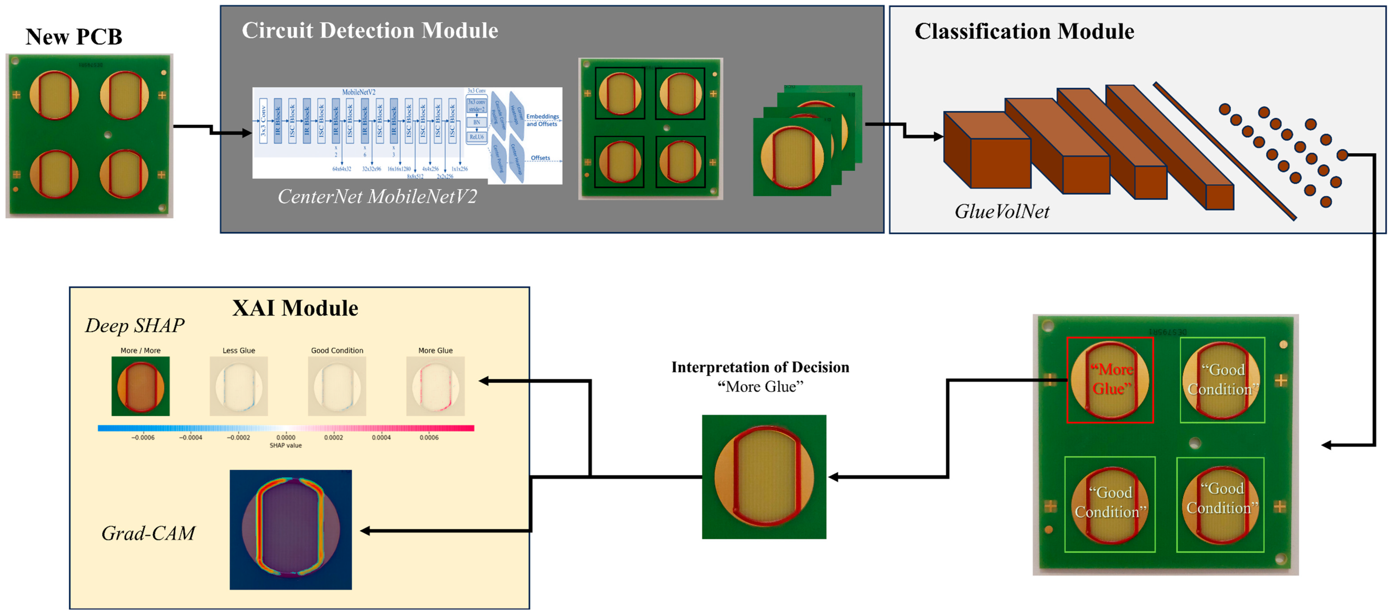
Figure 1. The proposed XAI framework for glue quality inspection. It consists of sequential processing steps for detecting and classifying circuits based on the glue volume. Finally, XAI visualizations are provided for explainability.
Applsci 15 09061 g001
Figure 2. The development stages of the proposed framework.
Applsci 15 09061 g002
Figure 3. The top panels (a) depict the original dataset that was used in this work, highlighting the PCB position within the frame (left figures) and the differences in glue line thickness among classes (right figures), with the electronics layout covered. The bottom panels (b) present the dataset that was prepared for public dissemination without disclosing sensitive information. In (b), the raw image of the PCB is presented on the left, whereas on the right, PCB circuits from the defined classes are exhibited. In this case, the glue is placed perimetrically in the circuit.
Applsci 15 09061 g003
Figure 4. The architecture of the proposed GlueVolNet for classification.
Applsci 15 09061 g004
Figure 5. The applied Grad-CAM method in three testing samples of different glue volume classes. The jet colormap from Matplotlib was employed to visualize the heatmap activations, with blue denoting regions exhibiting negligible activation and red indicating regions exerting the greatest influence on the model’s decision.
Applsci 15 09061 g005
Figure 6. The SHAP values or four testing images. On the left column is the original image, whereas the next columns present the SHAP values for each class. Above the original image, the actual and the predicted class are given.
Applsci 15 09061 g006
Table 1. Results of the comparison of circle Hough transform and CenterNet MobileNetV2.
MethodAccuracymAP@IoU{0.5:0.95}mAP@0.5 IoUmAP@0.75 IoUDetection Time (CPU)Detection Time (GPU)
Circle Hough Transform100%---1 s-
CenterNet MobileNetV2-90%100%100%0.17 s0.10 s
Table 2. Classification metrics comparison for the examined models in the test dataset (the best metrics are bolded).
ModelAccuracyF1-ScorePrecisionRecall
MobileNetV20.697 ± 0.1000.492 ± 0.0660.608 ± 0.1040.490 ± 0.066
VGG160.886 ± 0.0410.819 ± 0.1140.824 ± 0.1220.823 ± 0.108
VGG190.904 ± 0.0910.876 ± 0.0920.890 ± 0.0740.879 ± 0.100
ResNet500.892 ± 0.0380.843 ± 0.0410.901 ± 0.0330.826 ± 0.059
Branch-ResNet CNN0.881 ± 0.0480.733 ± 0.1300.767 ± 0.1610.742 ± 0.113
GlueVolNet0.922 ± 0.0280.887 ± 0.0680.894 ± 0.0620.877 ± 0.066
Table 3. Classification report of an average run for the GlueVolNet.
PrecisionRecallF1-ScoreSupport
Less glue0.871.00.9313
Good condition1.00.60.7515
More glue0.891.00.9432
Micro average0.90.90.960
Macro average0.920.870.8760
Table 4. Confusion matrix of an average run for the GlueVolNet.
PrecisionRecallF1-Score
Less glue1300
Good condition294
More glue0032
Table 5. Classification report of an average run for the GlueVolNet (using sliding window DA).
PrecisionRecallF1-ScoreSupport
Less glue0.990.920.961024
Good condition0.880.690.771100
More glue0.860.980.922112
Micro average0.890.890.894236
Macro average0.910.870.884236
Table 6. Confusion matrix of an average run for the GlueVolNet (using sliding window DA).
PrecisionRecallF1-Score
Less glue947770
Good condition12748340
More glue2332077
Table 7. Average processing times (in seconds).
Circuit Detection Classification Grad-CAM HeatmapsTotal
Desktop CPU0.140.090.512.36
Desktop GPU0.100.060.371.88
Jetson Nano CPU0.860.982.6811.35
Disclaimer/Publisher’s Note: The statements, opinions and data contained in all publications are solely those of the individual author(s) and contributor(s) and not of MDPI and/or the editor(s). MDPI and/or the editor(s) disclaim responsibility for any injury to people or property resulting from any ideas, methods, instructions or products referred to in the content.