Article

An Integrated CNN-BiLSTM-Adaboost Framework for Accurate Pipeline Residual Strength Prediction

1
College of Mechanical and Electronic Engineering, Nanjing Forestry University, Nanjing 210037, China
2
School of Information Science and Engineering, Shandong Normal University, Jinan 250300, China
3
School of Control Science and Engineering, Shandong University, Jingshi Road, Jinan 250061, China
*
Author to whom correspondence should be addressed.
Appl. Sci. 2025, 15(16), 9059; https://doi.org/10.3390/app15169059 (registering DOI)
Submission received: 2 July 2025 / Revised: 30 July 2025 / Accepted: 15 August 2025 / Published: 17 August 2025
(This article belongs to the Section Computing and Artificial Intelligence)

Abstract

To ensure the economy and safety of the pipelines, the study of the residual strength of corrosion pipelines is key to determining whether the pipelines can continue to operate. There is often a conflict between accuracy and convenience. Artificial intelligence algorithms offer the advantages of high accuracy and ease of use. Therefore, research on the prediction of the residual strength of corroded pipelines using artificial intelligence algorithms is of great significance. CNN and LSTM algorithms are often used to predict the remaining strength of pipelines. However, single CNN models perform poorly in handling time-series data, while LSTM and BiLSTM models also have limitations in processing high-dimensional spatial features. In this article, a pipeline residual strength prediction model based on the CNN-BiLSTM-Adaboost algorithm is proposed. Correlation analysis was used to evaluate the influencing factors of the pipeline’s residual strength, and the CNN algorithm parameters were optimized using BiLSTM and AdaBoost algorithms. The proposed CNN–BiLSTM–AdaBoost evaluation method achieves a significantly improved prediction accuracy for pipeline residual strength, with an average relative error of 4.694%. Our method reduces the predictive error by 28.901%, 43.391%, and 40.753% relative to ASME B31G, DNV RP F101, and PCORRC. This model can predict the residual strength of pipelines conveniently and accurately, minimizing losses caused by corrosion.

1. Introduction

Pipeline transportation is an important mode of transportation in China. Due to the large volume of detected data and the reliance on manual interpretation for defect identification, traditional methods are time-consuming, labor-intensive, and prone to errors such as false detections and missed detections. Therefore, there is an urgent need to develop intelligent defect identification methods to improve defect detection efficiency. If the residual strength of pipelines can be accurately predicted and effectively maintained, the occurrence of major accidents, such as oil and gas leaks, will be reduced, leading to minimized economic losses and environmental protection.
In recent years, researchers have increasingly adopted data-driven intelligent approaches for prediction. Oh et al. [1] explored the use of deep neural networks in predicting the burst pressure of API 5L Class X pipes, validating the model experimentally. Lu et al. [2] applied a correlation vector machine enhanced by a multi-objective optimization algorithm to predict burst pressure in corroded pipes, evaluating the model’s accuracy and stability through case studies. In another study [3], a hybrid data-driven model was employed to predict the residual strength of a single-point corroded pipeline, utilizing principal component analysis to optimize the input data. Ma et al. [4] introduced a neural network model guided by theoretical principles for predicting burst pressure in corroded pipelines, combining traditional burst pressure prediction formulas with empirical formula knowledge. Experimental and finite element simulations using open datasets confirmed the model’s superior prediction accuracy compared to benchmark models. Lu et al. [5] employed various machine-learning models [6], including regression, tree-based artificial neural networks, and kernel-based models, to predict corrosion depth in pipelines. Chen et al. [7] used an artificial neural network to predict residual strength in corroded pipes, employing a modified linear unit (ReLU) activation function to reduce neurons due to limited training data. However, most current research on pipeline residual strength prediction focuses on improving and applying pipeline strength evaluation formulas and conducting experimental tests using finite element analysis, while exploration of algorithms remains limited.
The convolutional neural network (CNN) [8,9,10], as a typical deep neural network, has been introduced into pipeline leakage diagnosis due to its unique convolutional structure, weight sharing, local connection, and strong autonomous feature extraction ability. Research by numerous scholars has shown that CNN exhibits a good classification prediction performance in pipeline leakage detection. Chuang et al. [11] proposed a CNN-based leakage detection method for groundwater pipelines, using the Mel frequency cepstrum coefficient of the leakage acoustic signal as the input and the presence or absence of leakage in the pipeline as the output. The model achieved a classification accuracy of 98%. Zhou et al. [12] proposed a one-dimensional convolutional neural network (TL1DCNN) method with integrated transfer learning to accurately detect and locate leaks using small samples, employing particle swarm optimization (PSO) to optimize the base learner’s weights. Kang et al. [13] fused one-dimensional convolutional neural networks with Support Vector Machines (SVMs) [14,15,16] to propose an image-based leakage detection and location algorithm for water supply networks, achieving a leak detection accuracy of 99.3%. Cody et al. [17] proposed a pipeline leakage detection method based on CNN combined with a mutation autoencoder, classifying hydroacoustic data and achieving a classification accuracy of 97.2%. Guo et al. [18] used the leakage spectrum to describe the leakage signal characteristics and established a time–frequency convolutional neural network model to identify leakage signals, achieving an average classification accuracy of 98% under different signal-to-noise ratios. However, these algorithms still need optimization to further improve accuracy and feasibility. While CNN has been successfully applied in computer vision and other fields for efficiently learning features from image and spatial data, it remains relatively inadequate in capturing long-term temporal dependencies in time-series data, making them less effective in handling complex temporal data [19].
To overcome this limitation, Long Short-Term Memory (LSTM) networks [20] have been widely applied in time-series prediction. LSTM effectively addresses the vanishing gradient problem faced by traditional recurrent neural networks (RNNs) [21] when handling long-term sequential data through the introduction of memory units and gating mechanisms. Bidirectional long and short-term neural network (BiLSTM) [22,23,24] further enhances LSTM’s performance by processing both past and future inputs simultaneously. However, while BiLSTM excels in temporal modeling, it still falls short in handling high-dimensional spatial data, where CNN performs more effectively.
Despite the complementary strengths of CNN and BiLSTM, both models individually face challenges when applied to complex real-world scenarios. CNN is limited in its ability to capture long-term dependencies, while BiLSTM struggles with high-dimensional spatial feature extraction. To address these limitations, the Adaptive Boosting (AdaBoost) [25] algorithm can be employed to combine the strengths of both models and further enhance predictive performance.
AdaBoost is widely used in various machine-learning tasks, excelling in classification and regression problems. Its main advantage is the ability to enhance overall model performance by combining multiple weak classifiers, making AdaBoost robust when dealing with noisy and imbalanced data [26]. Compared to using CNN alone, AdaBoost compensates for CNN’s limitations in handling complex patterns, particularly in capturing long-term dependencies in time-series data. By combining AdaBoost with CNN, the model’s learning capacity and generalization performance are optimized, improving the accuracy of pipeline residual strength prediction. Thus, integrating the AdaBoost algorithm with CNN for pipeline residual strength prediction leverages CNN’s powerful feature extraction capabilities while enhancing the robustness and accuracy of the model through AdaBoost’s ensemble learning strategy, resulting in more reliable predictions in practical applications.
In this study, we propose a CNN-BiLSTM-Adaboost model that combines the spatial feature extraction capabilities of CNN, the temporal dependency capture of BiLSTM, and the ensemble learning strategy of Adaboost. The Adaboost algorithm improves the overall robustness and generalization of the model by iteratively adjusting sample weights, focusing on misclassified samples, and optimizing the model ensemble. In this combined framework, CNN first extracts local spatial features from pipeline data, BiLSTM captures the temporal dependencies, and Adaboost optimizes the overall prediction performance through model integration. We compared the predictive effectiveness of various algorithms, including CNN, LSTM, BiLSTM, BiLSTM-Adaboost, CNN-LSTM, CNN-BiLSTM, and CNN-BiLSTM-Adaboost. Through correlation analysis, we verified the fit between the predictions of intelligent algorithms and actual outcomes. We analyzed the correlation between inner diameter, wall thickness, corrosion defect depth, defect length, and burst pressure under different optimization algorithms. Based on these results, we employed CNN using the optimal penalty factor and kernel function, applying it to predict the residual strength of 93 corroded pipelines. By comparing the average relative error and the number of non-conservative points in the predictions, the CNN-BiLSTM-Adaboost algorithm with the highest accuracy was ultimately selected. A comparison between the CNN-BiLSTM-AdaBoost algorithm and standard evaluation methods confirmed the feasibility of intelligent algorithms in predicting pipeline residual strength. Compared to traditional pipeline residual strength evaluation standards, this intelligent algorithm is not only accurate but also easy to implement.

2. Methods

2.1. Residual Strength Prediction Based on Correlation Analysis

A correlation analysis model [27] in Matlab software (Matlab R2023a) is established which involves analyzing data in numerical form as Matlab algorithms primarily operate with numerical data. Therefore, the data analyzed in this study is presented in numerical form, and some of the influencing factors transform preprocessing. In the course of this research, the main factors considered include pipeline inner diameter, pipeline wall thickness, defect depth, defect length, and actual burst pressure. All data are derived from the literature, and the data sources are presented in Table 1, with partial pipeline burst pressure data shown in Table 2.
The data was input into the correlation analysis model for analysis, and the results obtained are shown in the following Figure 1. It can be observed that factors such as pipeline diameter, pipeline wall thickness, defect depth, and defect length are correlated with the actual burst pressure of the pipeline. As depicted in Figure 1, pipeline diameter and pipeline wall thickness are positively correlated with the actual burst pressure, at 0.01029 and 0.3825, while defect length and defect depth show a negative correlation with the pipeline burst pressure, −0.1228 and −0.2166, respectively. Among all influencing factors, the pipeline wall thickness has a relatively significant impact on the residual strength of the pipeline.
Prior to model training, the data underwent a four-step preprocessing pipeline: (1) missing value check and removal, (2) unit normalization, (3) Z-score standardization, (4) correlation analysis to verify feature relevance.

2.2. Principle of the CNN-BiLSTM-Adaboost Algorithm and Parameter Setting

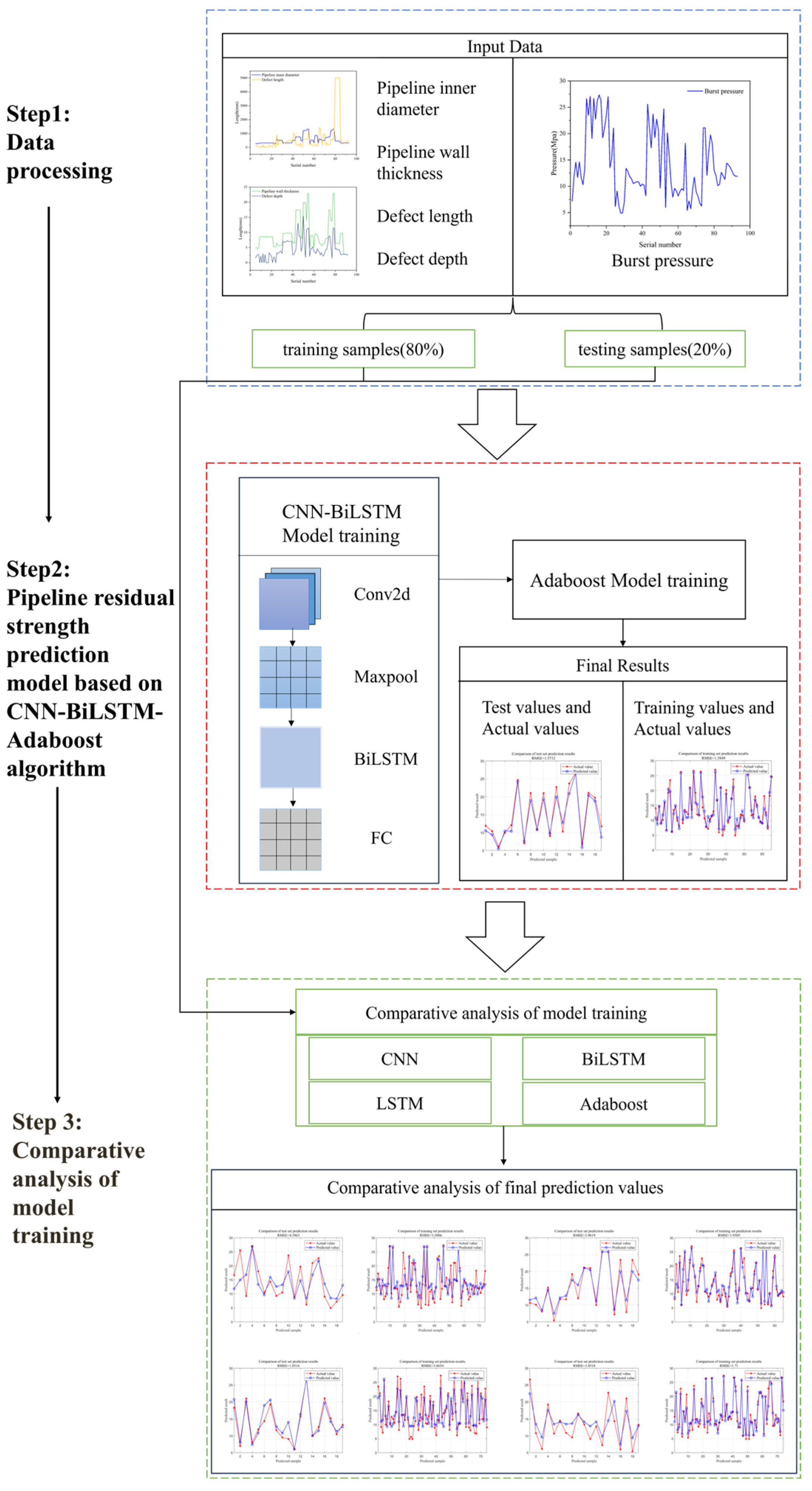
In the context of predicting the residual strength of pipelines, we proposes a hybrid model that integrates convolutional neural networks, bidirectional Long Short-Term Memory networks, and the Adaboost algorithm, referred to as the CNN-BiLSTM-Adaboost algorithm. This approach leverages the strengths of spatial feature extraction, temporal dependency modeling, and ensemble learning to enhance prediction accuracy and model robustness. The dataset was randomly partitioned into training and testing subsets, with 80% of the samples allocated for training and the remaining 20% for testing, ensuring a balanced evaluation of model performance. The strategy diagram of prediction is shown in Figure 2.

2.2.1. CNN Algorithm

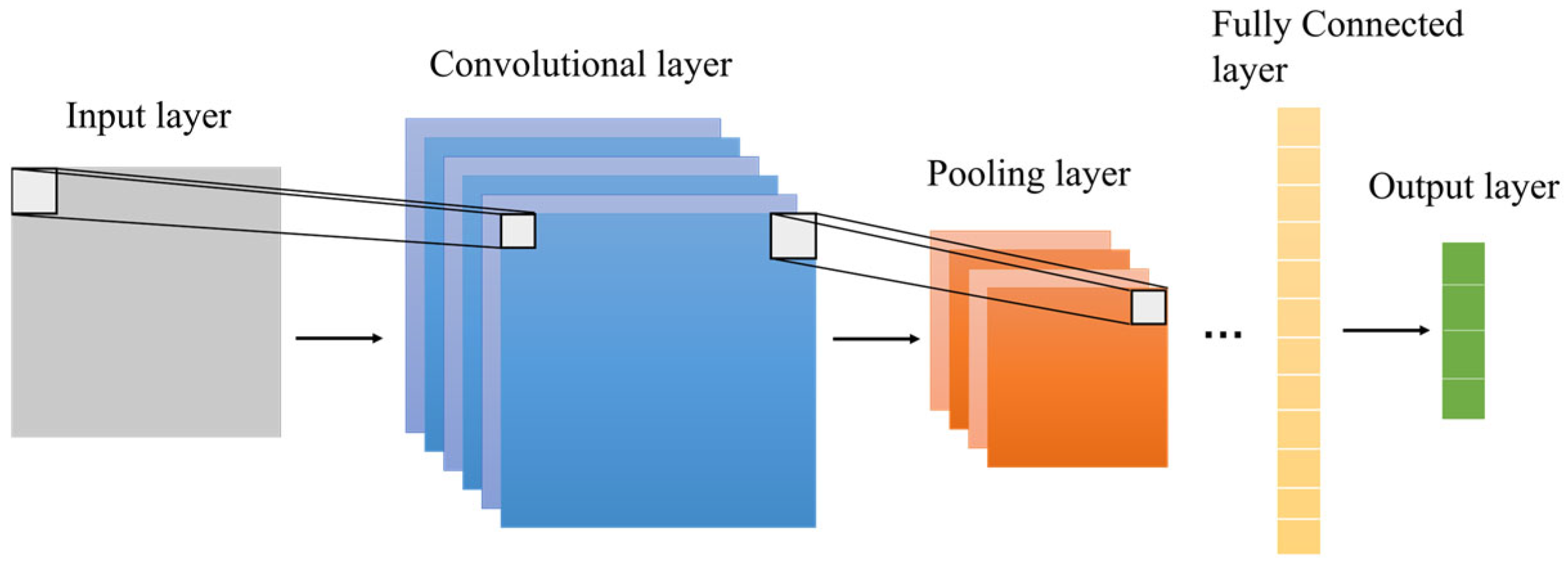
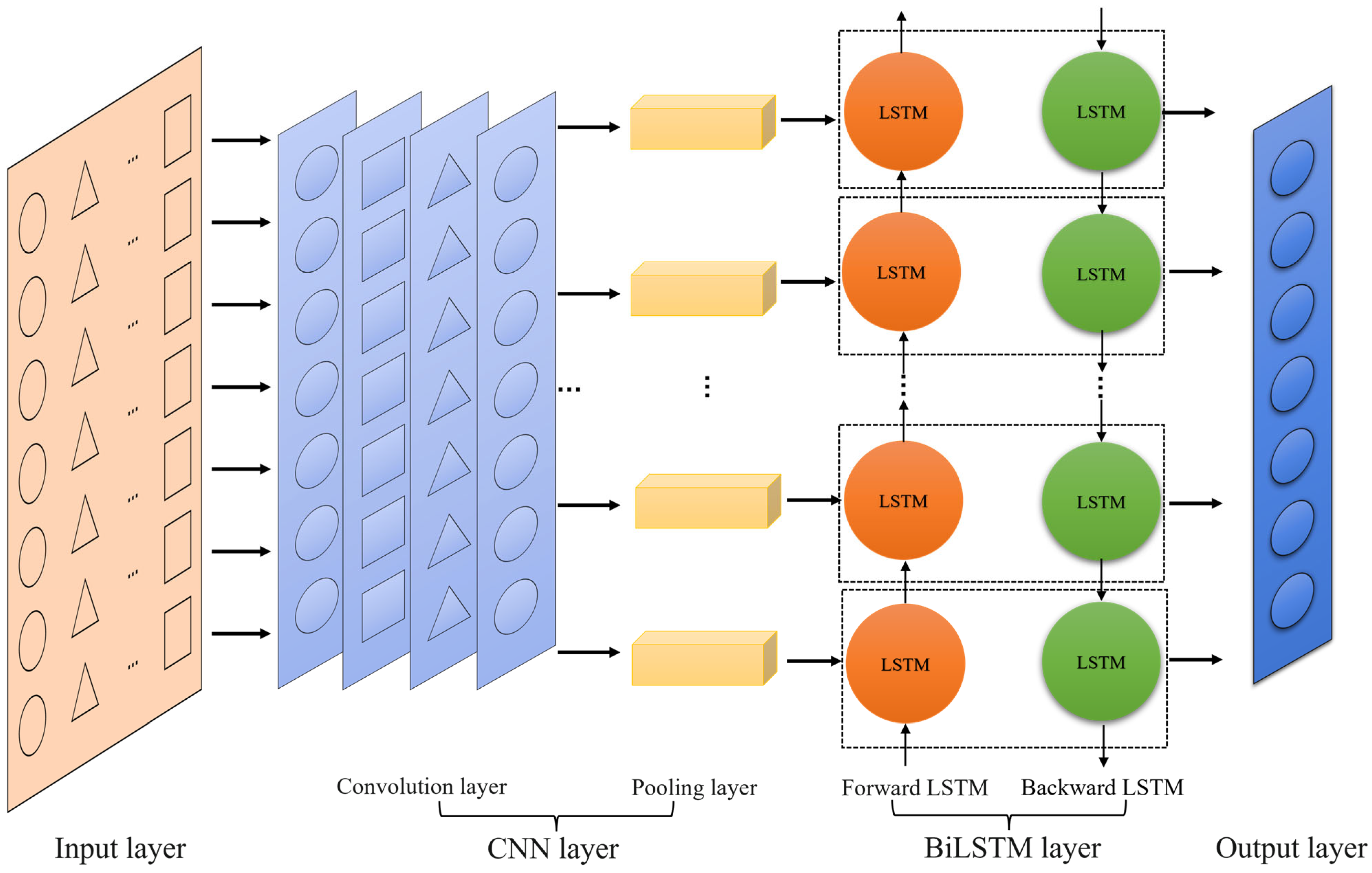
CNN is a deep neural network architecture consisting of convolutional layers, pooling layers, and fully connected layers. Its basic structure is shown in Figure 3. Convolution operations are central to the functionality of a CNN. In the convolutional layer, the network analyzes input data through convolution operations using a set of learnable filters known as convolutional kernels. The operation of the convolutional layer is expressed as
C i = f w i × x i + b i
where x i denotes the input of the convolutional layer, C i is the output feature map of layer iii, w i is the weight matrix of the convolution, × denotes the dot product operation, b i is the bias vector, and f is the activation function [33].
Pooling operations are utilized to decrease the spatial dimensions of the feature map while preserving critical features. Typical pooling operations include max pooling and average pooling. The pooling layer operation is shown as
γ c i , c i 1 = max c i , c i 1
p i = γ c i , c i 1 + β i
where γ denotes the maximum pooling function, β i is the deviation, and p i is the output of the maximum pooling layer. The feature maps obtained through pooling operations are transferred to the fully connected layer, which computes the final output vector [34].
The fully connected layer resides at the apex of the network, transforming features extracted by preceding convolutional and pooling layers into the ultimate output. In this layer, every neuron is connected to all neurons in the preceding layer. The operation of the fully connected layer is expressed as
y i = f t i p i + δ i
where y i is the final output vector, δ i is the bias, and t i is the weight matrix.
The input data, X = x 1 , x 2 , , x n , undergoes normalization to scale the values between 0 and 1 using the min–max normalization technique:
X = X X min X max X min
Given an input X R H × W × C , where H is the height, W is the width, and C is the number of channels, the feature map generated by the convolution operation is
H i , j , k = σ m = 1 M n = 1 N W m , n , k X i + m 1 , j + n 1 , k + b k
Here, H i , j , k represents the k -th feature map at position ( i , j ) , W m , n , k denotes the weight matrix of the convolution kernel, is the bias term. The ReLU activation function, σ ( x ) = max ( 0 , x ) , introduces nonlinearity into the network, enhancing the model’s ability to capture complex patterns [35].
Subsequently, a max-pooling layer with a pooling size of 3 × 1 and a stride of 1 reduces the dimensionality of the extracted features, summarized as
H i , j , k = max H i , j , k , H i + 1 , j , k , H i + 2 , j , k

2.2.2. LSTM Algorithm

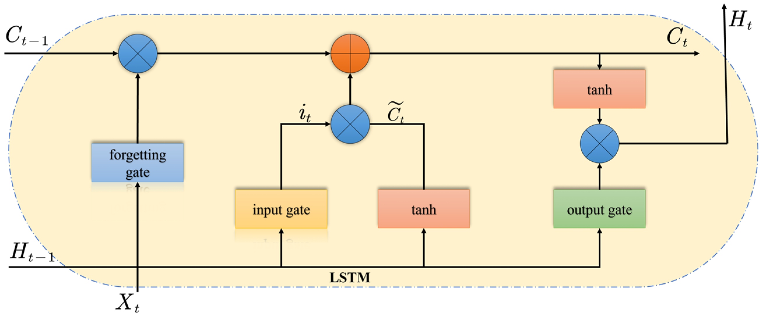
LSTM is a special type of recurrent neural network (RNN) designed to overcome the gradient vanishing and exploding problems that traditional RNNs face when dealing with long-term dependencies. LSTMs effectively store and update information through the introduction of memory cells and gating mechanisms. The core structure of LSTM includes an input gate, a forget gate, and an output gate. Its basic structure is shown in Figure 4.
The key equations governing the operations within LSTM are as follows:
1.
Input Gate
H i , j , k = max H i , j , k , H i + 1 , j , k , H i + 2 , j , k
where i t is the output of the input gate, σ is the Sigmoid activation function, h t 1 is the hidden state from the previous time step, and x t is the input at the current time step [36].
2.
Forget Gate
f t = σ w f × h t 1 , x t + b f
f t is used to control whether the memory from the previous time step should be forgotten [37].
3.
Candidate Cell State
C t ˜ = tanh w c × h t 1 , x t + b c
4.
Current Cell State
C t = f t × C t 1 + i t × C t ˜
5.
Output Gate
σ t = σ ( w o × h t 1 , x t + b o )
6.
Current Hidden State
S t = σ t × tanh C t
In these equations, C t represents the cell state at the current time step, while S t denotes the hidden state.

2.2.3. BiLSTM Algorithm

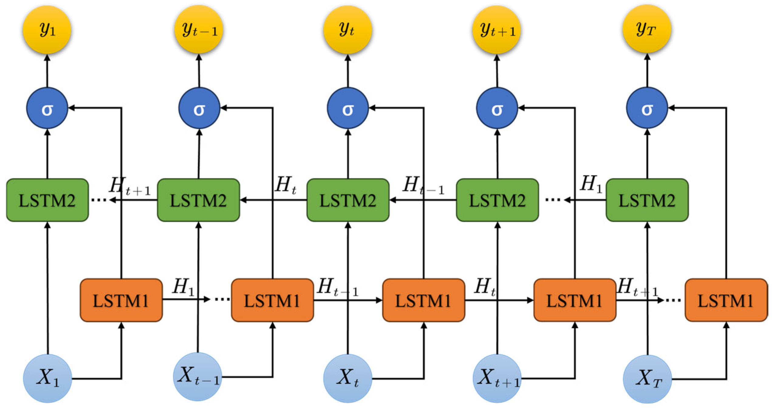
BiLSTM build upon LSTM by incorporating a reverse LSTM layer to process time-series data in both forward and backward directions [38]. Unlike traditional LSTM, which only utilizes past information, BiLSTM enhances context understanding by using two LSTMs at each time step—one for past inputs and one for future inputs. Its basic structure is shown in Figure 5.
The BiLSTM network is capable of handling temporal dependencies in sequential data, with its bidirectional structure allowing the model to capture both past and future contextual information. For a given time-series input, the forward and backward hidden states in BiLSTM are computed as follows:
  • Forward LSTM
h t = L S T M F t , h t 1
  • Backward LSTM
h t = L S T M F t , h t 1
The final output of the BiLSTM H t is the concatenation of the forward and backward hidden states:
H t = h t h t
where denotes the concatenation operation. This approach ensures that the model leverages information from both past and future sequences, thus improving the prediction accuracy [39]. The BiLSTM output is passed through a fully connected layer, converting the hidden states into output predictions, followed by a regression layer that maps these predictions to the actual values, as shown in the following equation:
y = W f c H t + b f c
where W f c and b f c are the weights and biases of the fully connected layer, and y is the final output.
The model optimization is performed using the Adam optimizer, which adjusts the learning rate dynamically during training. The learning rate starts at α = 0.01 and decays by a factor of 0.01 every 70 epochs, enhancing the model’s convergence. The structure of CNN-BiLSTM is shown in Figure 6.
Each pipeline sample was structured as a 1 × 4 vector containing geometric features. These were processed as 1D feature maps by the CNN with kernel size of 1. No time-series simulation was applied; all data were static and literature-derived.
To enable BiLSTM processing, each feature vector was reshaped into a sequence of four pseudo-time steps. This structure allowed the model to learn inter-feature relationships in a temporal fashion despite the data being static.
The CNN input is shaped as a 1 × 4 × 1 tensor. After convolution and pooling, a 4 × 1 sequence is passed to BiLSTM, producing a 64-dimensional feature vector. This vector is input into AdaBoost, which outputs a scalar prediction of residual strength. The parameters used in the CNN-BiLSTM method are listed in Table 3.

2.2.4. Adaboost Algorithm

Adaboost is an ensemble learning algorithm that combines multiple weak classifiers to form a strong classifier. The core idea of Adaboost is to iteratively adjust the weights of training samples, giving higher weights to those samples that were misclassified in previous iterations, thus improving the overall classification accuracy. The Adaboost algorithm is employed to enhance the CNN-BiLSTM model by iteratively training multiple weak regressors and combining them into a strong predictor. Ten weak regressors (K = 10) are used.
In each iteration, given a weight distribution w i ( t ) , a weak classifier h ( t ) is trained, and its weighted error ε ( t ) is computed as
ε ( t ) = i = 1 n w i ( t ) g h ( t ) x i y i
where g { } is the indicator function, y i is the true label of sample i . The weight of the weak classifier is then calculated as
α ( t ) = 1 2 ln 1 ε ( t ) ε ( t )
Subsequently, if h ( t ) x i = y i , the weight distribution of the training samples is updated as
w i ( t + 1 ) = w i 2 1 ε ( t )
If h ( t ) x i y i , the weight distribution of the training sample is updated as
w i ( t + 1 ) = w i 2 ε ( t )
Finally, the output of Adaboost is the weighted voting result of all weak classifiers:
f ( T ) ( ) = t = 1 T α ( t ) h ( t ) ( )

2.2.5. CNN-BiLSTM-Adaboost Algorithm

  • Workflow of CNN-BiLSTM-Adaboost Algorithm
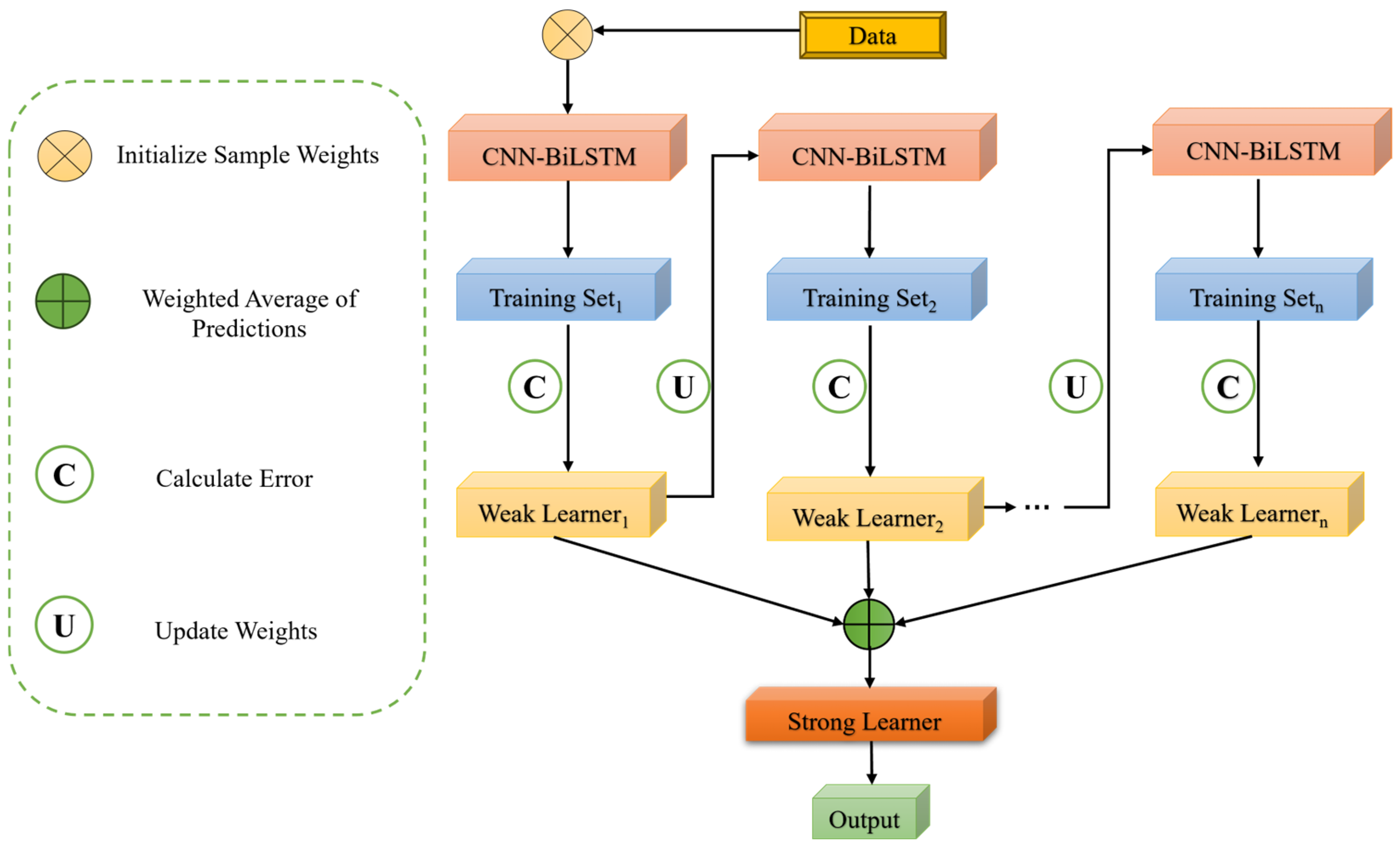
    The structure of CNN-BiLSTM-Adaboost is shown in Figure 7. The overall workflow of the CNN-BiLSTM-Adaboost algorithm is as follows.
    (a)
    Feature Extraction: CNN is utilized to extract spatial features from the input data, yielding the feature vector F C N N .
    (b)
    Sequence Modeling: The feature vector F C N N is then input into BiLSTM, which extracts temporal dependency features, resulting in the feature vector F B i L S T M .
    (c)
    Classification: Adaboost is employed to classify the feature vector F B i L S T M , producing the final prediction H ( F B i L S T M ) .
This hybrid model combines the spatial feature extraction capability of CNN, the temporal dependency modeling ability of BiLSTM, and the ensemble learning strength of Adaboost, making it highly effective for complex sequential data prediction tasks.
Figure 7. CNN-BiLSTM-Adaboost structure diagram.
Applsci 15 09059 g007
2.
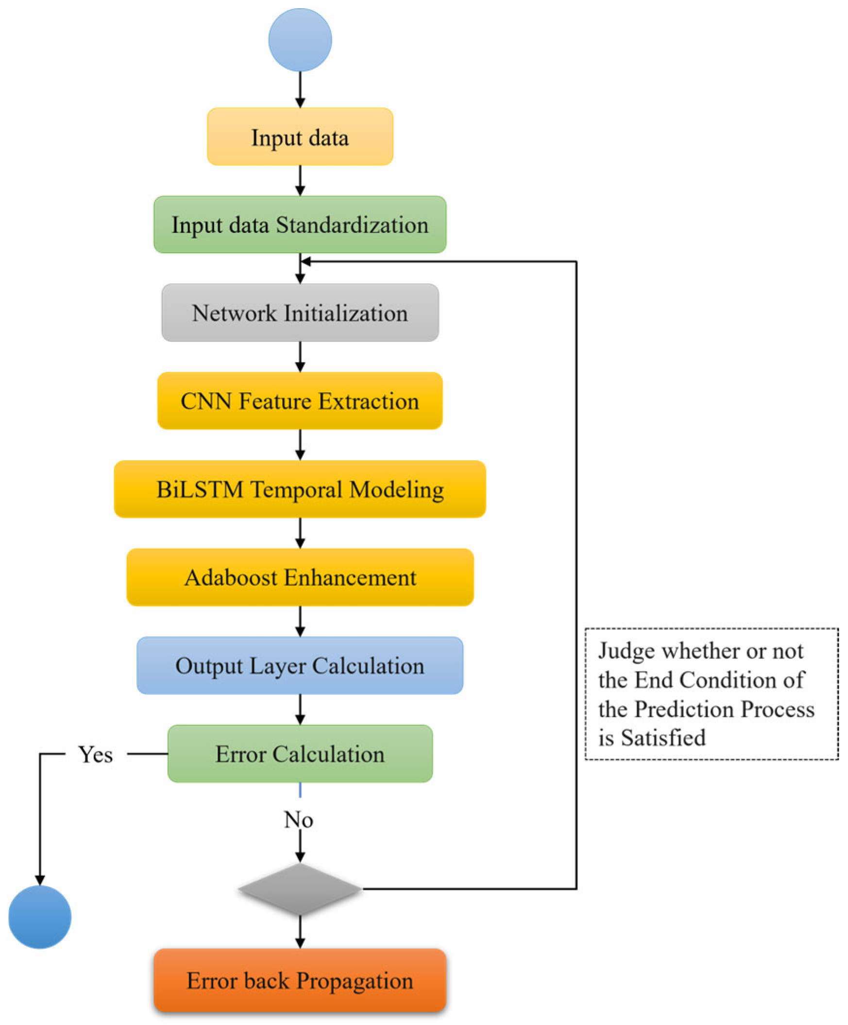
CNN-BiLSTM-Adaboost Training Process
The CNN-BiLSTM-Adaboost training process is shown in Figure 8, and the main steps are as follows.
(a)
Input Data: The data required for training the CNN-BiLSTM-Adaboost algorithm is fed into the model.
(b)
Data Standardization: As there is a large variance in the input data, z-score standardization is applied to normalize the input data, as shown in Formula (23).
y i = x i x ¯ s
where y i is the standardized value, x i is the input data, x ¯ is the average of the input data, and s is the standard deviation of the input data.
(c)
Network Initialization: The weights and biases of each layer of the CNN-BiLSTM-Adaboost model are initialized.
(d)
CNN Feature Extraction: The input data is passed through the convolution and pooling layers to extract local spatial features, resulting in a feature vector.
(e)
BiLSTM Temporal Modeling: The feature vector output from the CNN layer is passed through the BiLSTM layer, which processes the temporal dependencies in the sequential data via forward and backward LSTM networks, generating an output.
(f)
Adaboost Enhancement: The output from the BiLSTM layer is fed into multiple weak regressors, which are combined using the Adaboost algorithm to produce the final output.
(g)
Output Layer Calculation: The final output of the model is generated through a fully connected layer and a regression layer, mapping the Adaboost output to the final predicted value.
(h)
Error Calculation: The predicted value from the output layer is compared with the actual value for the dataset, and the corresponding prediction error is calculated. The error calculation metrics are the mean absolute percentage error (MAPE) and mean squared error (RMSE):
R M S E = 1 n i = 1 n y i ^ y i 2
M A P E = 1 n i = 1 n y ^ i y i y i × 100 %
(i)
End Condition Judgment: The training process is evaluated against termination conditions, which include completing a predetermined number of cycles, the weights falling below a certain threshold, or the prediction error rate being below a preset threshold. If any of these conditions are met, training is completed; otherwise, it continues.
(j)
Error Back Propagation: The calculated error is propagated backward through the network, updating the weights and biases of each layer. The process then returns to step 4 to continue training.
3.
CNN-BiLSTM-Adaboost Prediction Process
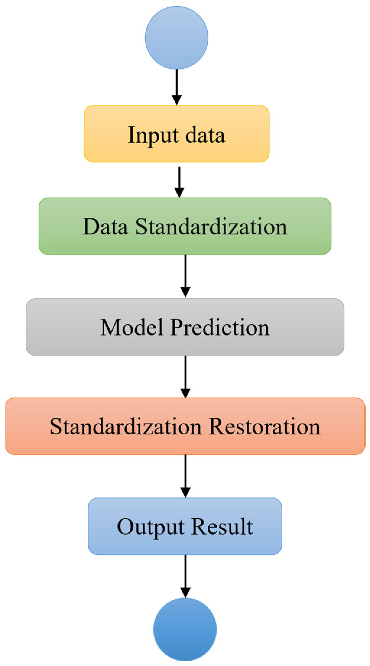
The precondition for the CNN-BiLSTM-Adaboost prediction is that the model has completed its training. The prediction process is shown in Figure 9, and the main steps are as follows.
(a)
Input Data: The input data required for prediction are fed into the model.
(b)
Data Standardization: The input data are standardized using the z-score method to ensure consistency with the data distribution during training.
(c)
Model Prediction: The standardized data are then fed into the trained CNN-BiLSTM-Adaboost model to generate the corresponding predicted output value.
(d)
Standardization Restoration: The predicted output value from the CNN-BiLSTM-Adaboost model is in a standardized form. It is restored to the original value using the following Formula (26).
x i = y i s + x ¯
where x i is the restored original value, y i is the output value from the CNN-BiLSTM-Adaboost model, s is the standard deviation of the input data, and x ¯ is the mean of the input data.
(e)
Output Result: The restored prediction results are then outputted, completing the prediction process.
Figure 9. Activity diagram of CNN-BiLSTM-Adaboost prediction process.
Applsci 15 09059 g009

3. Results and Discussion

3.1. CNN Algorithm for Residual Strength Prediction

In Matlab software, four combined models—BiLSTM-Adaboost, CNN-LSTM, CNN-BiLSTM, and CNN-BiLSTM-Adaboost—and the traditional CNN, LSTM, and BiLSTM models are constructed. The 93 sets of pipeline burst pressure and influencing factor data obtained from the literature are divided into two categories: the first category consists of 73 sets of data influencing pipeline residual strength and actual burst pressure, serving as the model’s training samples. The second category includes 20 sets of data influencing pipeline residual strength and actual burst pressure, serving as the model’s testing samples. Firstly, the BiLSTM-Adaboost, CNN-LSTM, CNN-BiLSTM, CNN-BiLSTM-Adaboost, and traditional CNN, LSTM, and BiLSTM models are individually trained using samples from the training set. Then, the trained models are used to predict the residual strength of the 20 testing samples, and the root mean square error of each predicted result is calculated. The average relative error of the 20 predicted samples is computed, and the fulfillment of conservatism requirements in the prediction results is statistically analyzed. The evaluation of the prediction results is presented in Table 4.
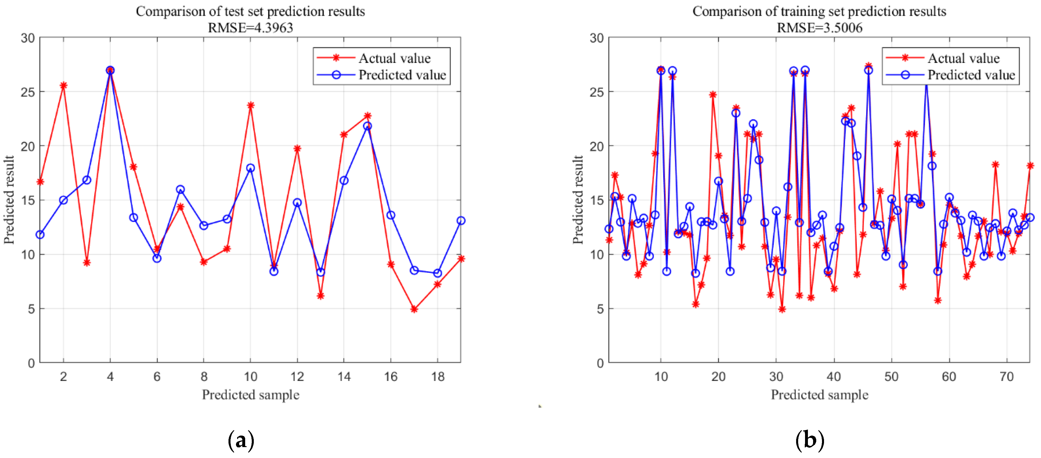
Figure 10 presents the results of the CNN model in predicting pipeline residual strength. By comparing the predicted and actual values for the training and testing sets, the fitting performance of the CNN model is displayed. While the CNN model captures part of the data trend, larger prediction errors are observed in some samples, particularly in the high-pressure regions, indicating the limitations of CNN in handling complex nonlinear data. The RMSE of the CNN model is 4.3963, reflecting significant errors, especially in the high-pressure regions.
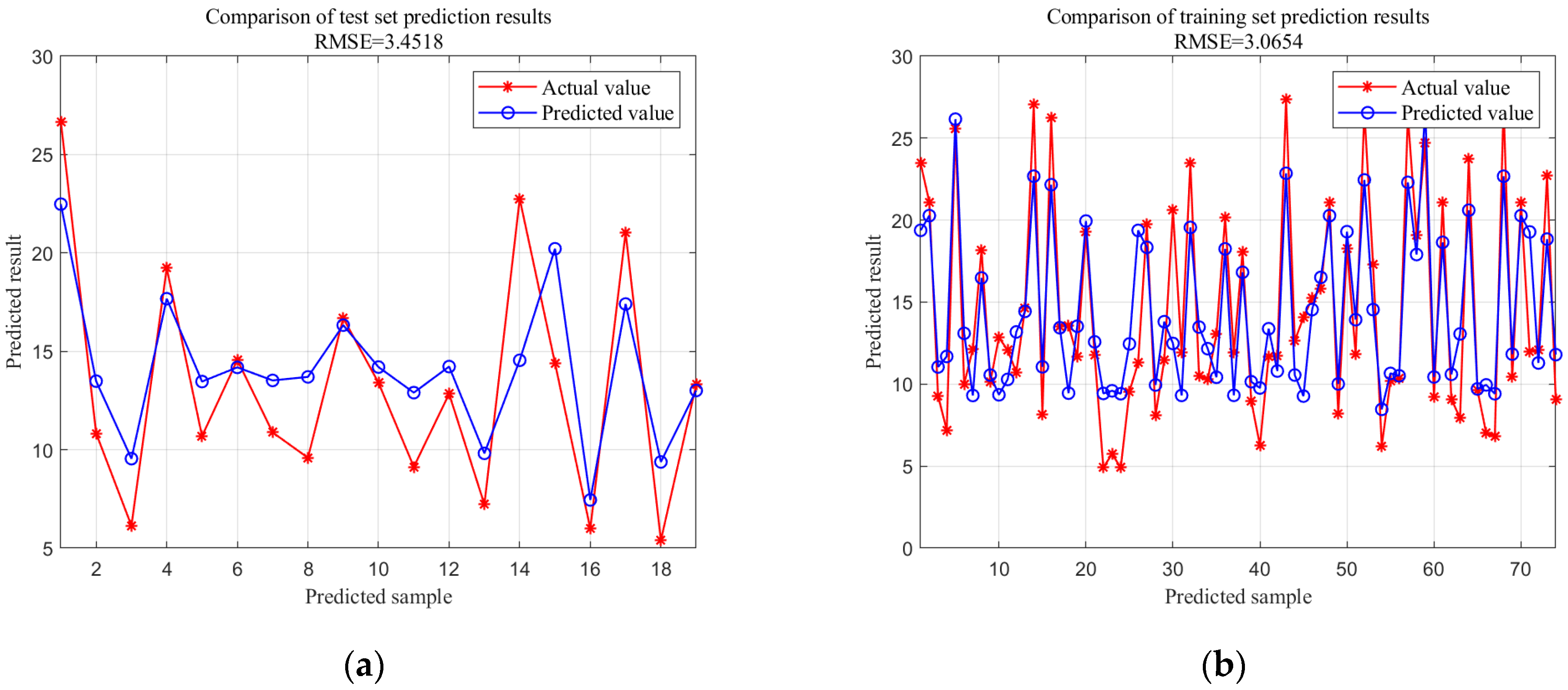
Figure 11 shows the prediction results of the BiLSTM-Adaboost model. It is evident that the BiLSTM-Adaboost model performs better than the CNN model in handling time-series data, with higher accuracy in the predicted values. The prediction accuracy is significantly improved across different data intervals, especially in the high-pressure regions, further validating the effectiveness of the AdaBoost ensemble learning strategy. The RMSE of the BiLSTM-Adaboost model is 3.0654, showing a substantial reduction in error compared to the CNN model and indicating a better fitting performance.
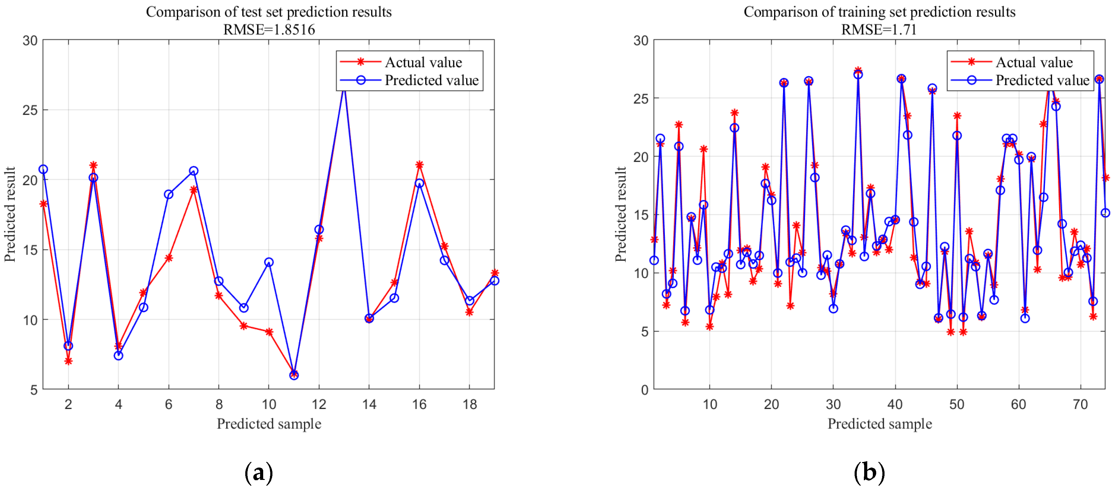
Figure 12 presents the prediction results of the CNN-LSTM model. Comparing the results of the CNN-LSTM model with other models, it can be seen that while LSTM captures temporal dependencies well, its prediction accuracy still needs improvement for certain complex nonlinear data points. The model’s performance in the high-pressure region is slightly inadequate, indicating that its overall fitting ability is still inferior to the BiLSTM-Adaboost model. The RMSE of the CNN-LSTM model is 1.8516, showing good performance in handling temporal dependency data.
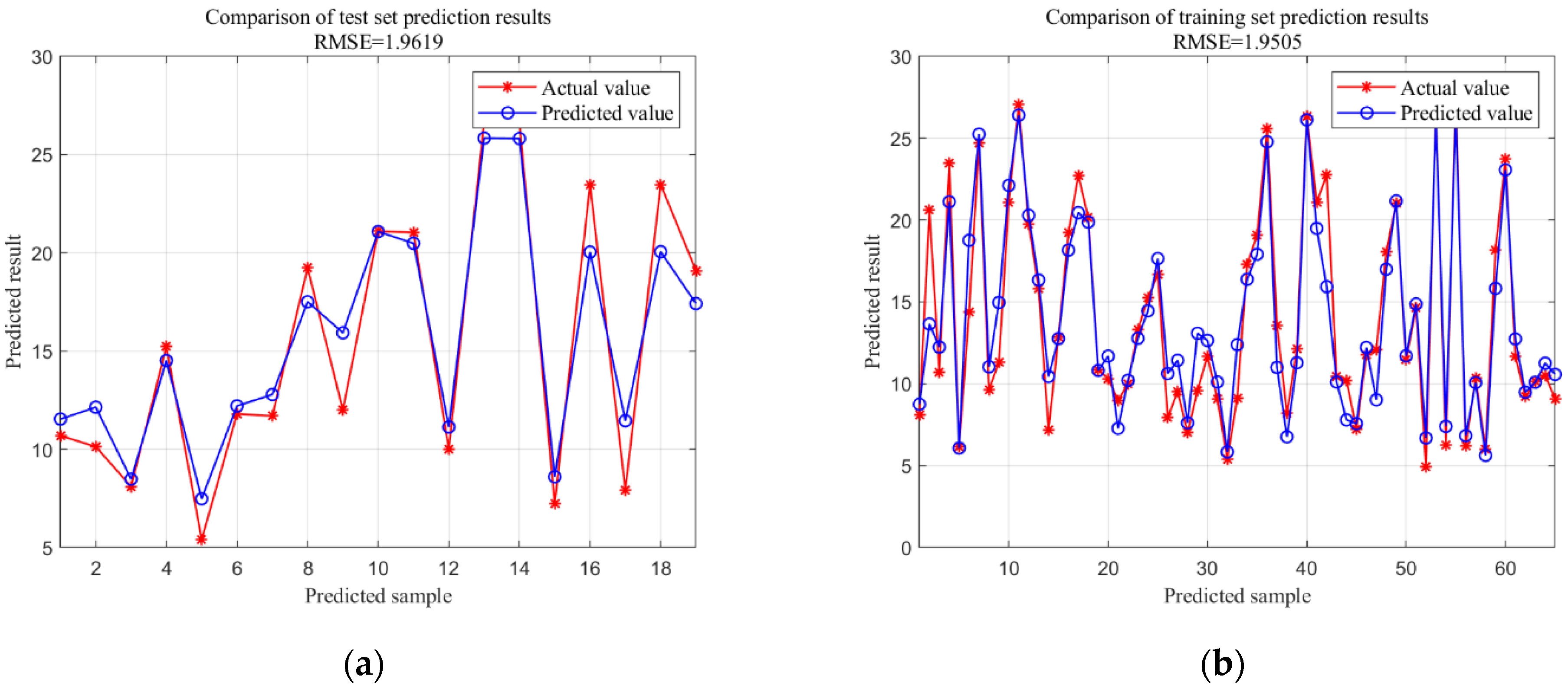
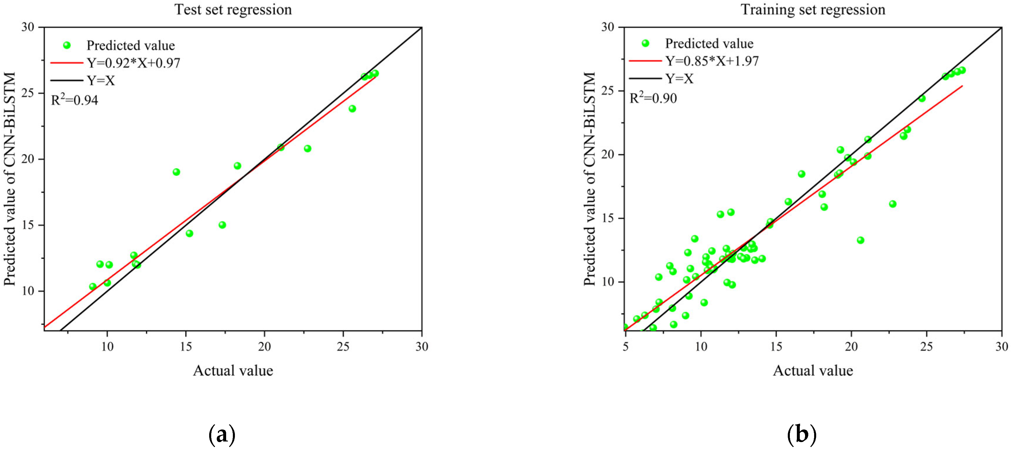
Figure 13 shows the prediction results of the CNN-BiLSTM model. Compared to the previous models, the CNN-BiLSTM model performs more consistently across different pressure ranges, with relatively lower prediction errors. The RMSE of the CNN-BiLSTM model is 1.9619, indicating a better overall performance than CNN and CNN-LSTM models.
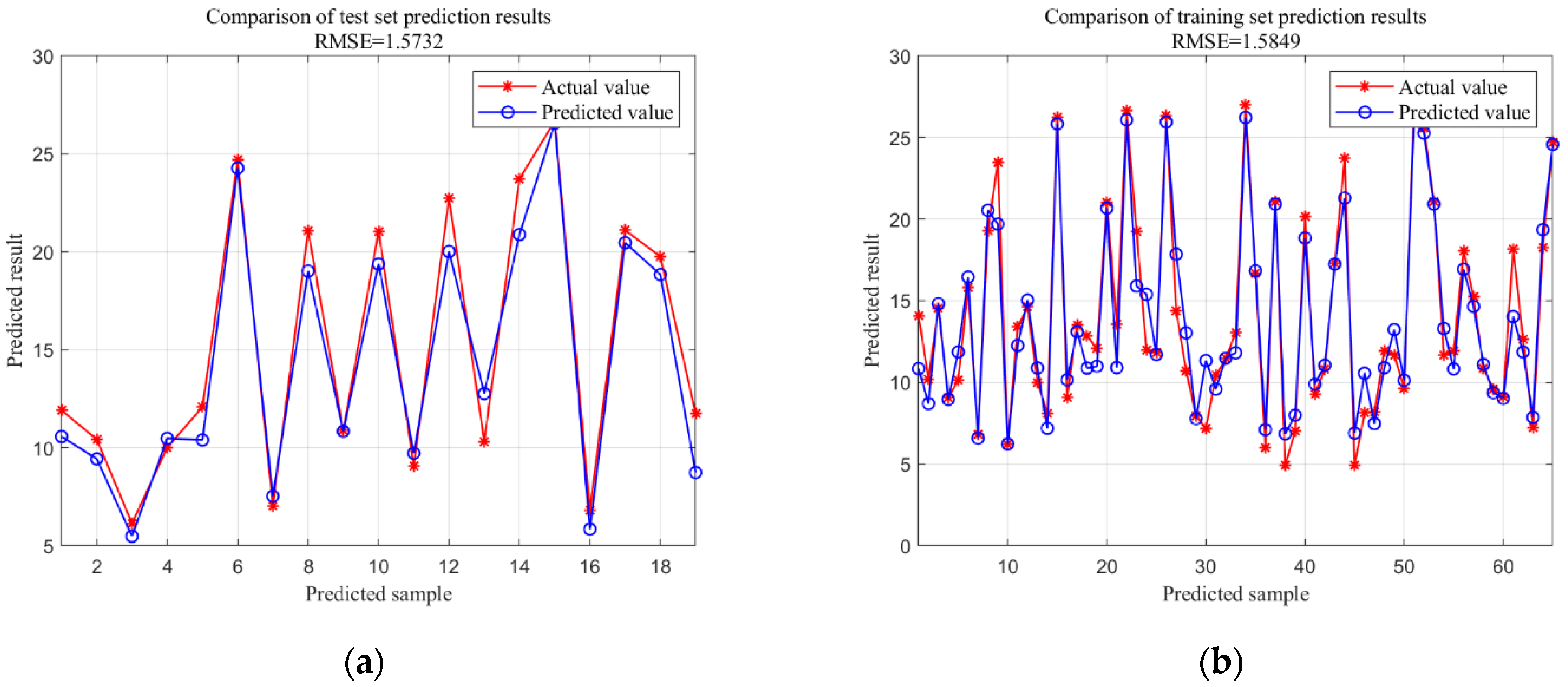
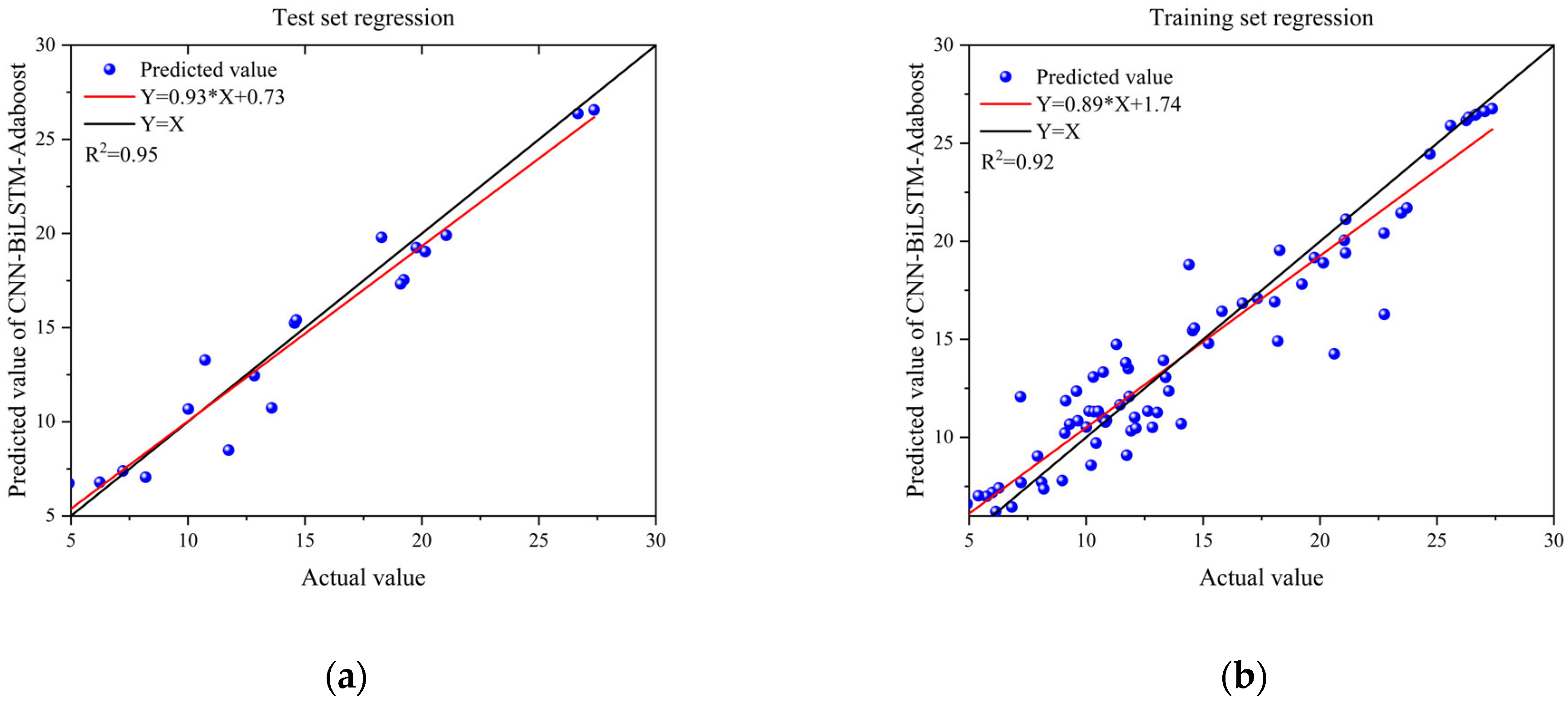
Figure 14 illustrates the prediction results of the CNN-BiLSTM-Adaboost model. A comparison with other models reveals that the CNN-BiLSTM-Adaboost model provides the most ideal fitting across various pressure ranges, particularly excelling in high-pressure predictions with minimal error. The RMSE of the CNN-BiLSTM-Adaboost model is 1.5732, the lowest among all models, demonstrating that the combination of CNN’s spatial feature extraction, BiLSTM’s temporal modeling, and AdaBoost’s ensemble learning significantly improves prediction accuracy.
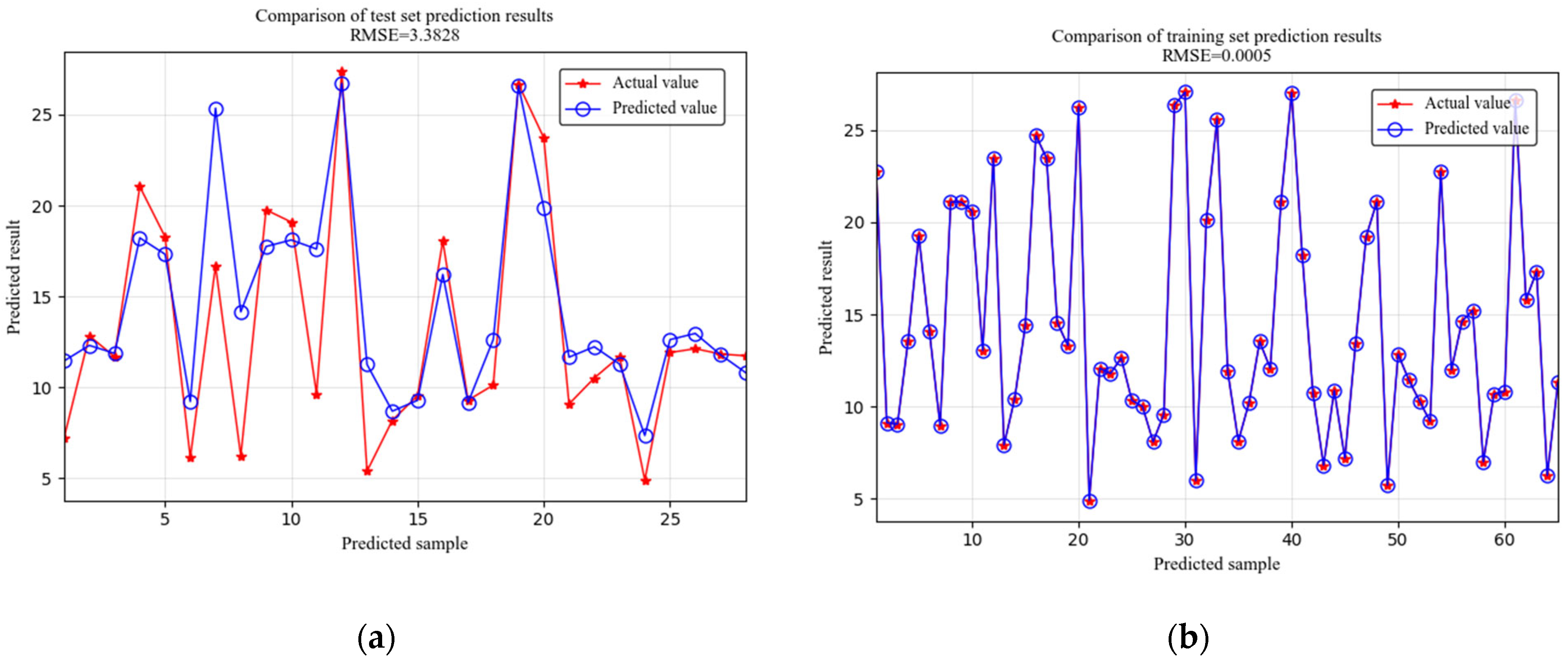
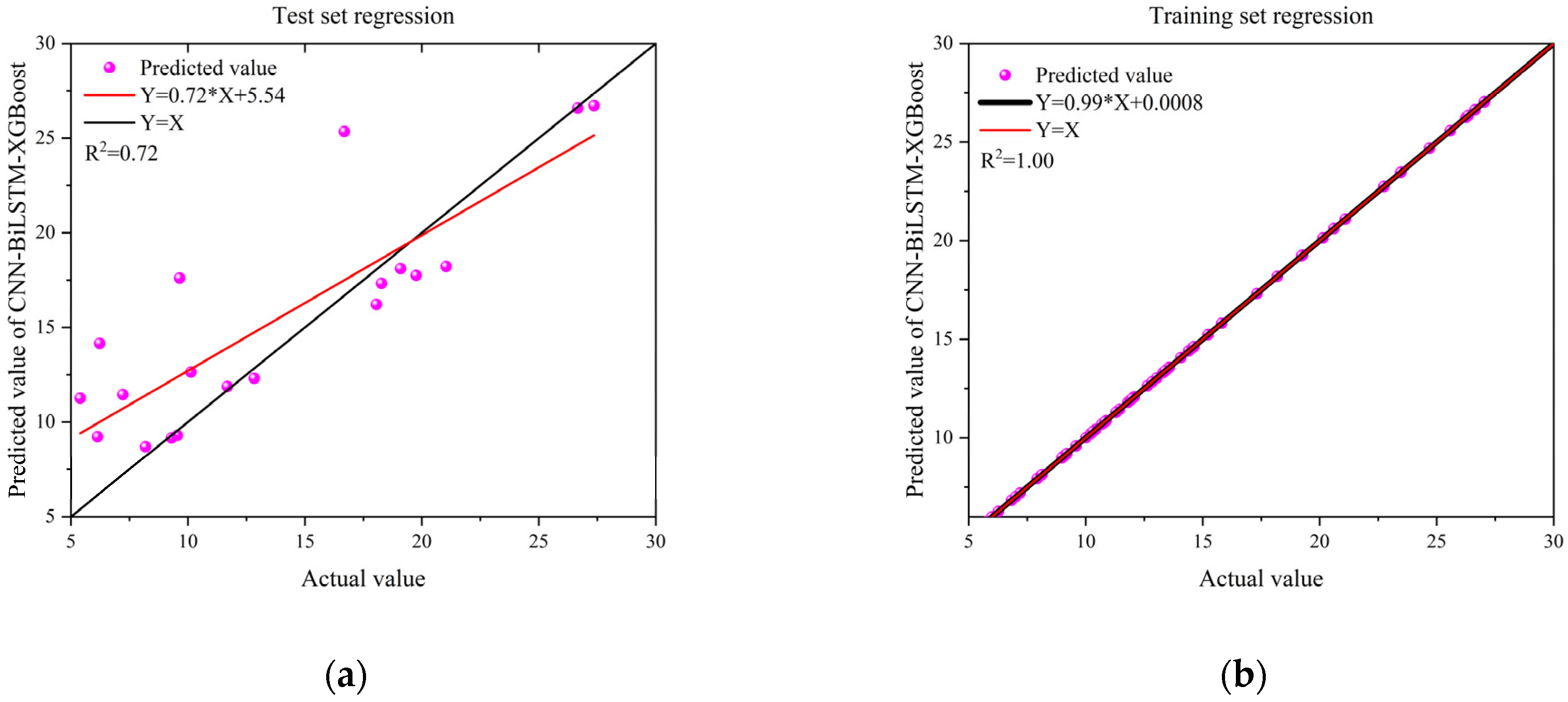
Figure 15 illustrates the prediction results of the CNN-BiLSTM-XGBoost model. The predicted values generally follow the actual values, showing the model’s ability to capture key trends in pipeline residual strength. With an RMSE of 3.3828, the model shows moderate error. The hybrid structure improves learning of spatial, temporal, and nonlinear features, providing a balanced but not optimal prediction solution.
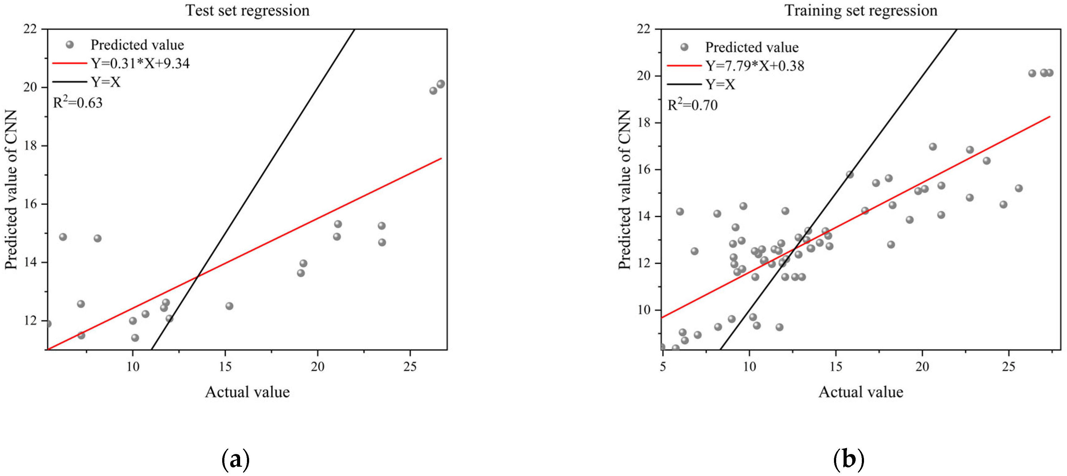
Figure 16 shows the linear fitting of the CNN model’s prediction results. Although the CNN model fits part of the data, the overall prediction performance is suboptimal. The R2 value of the CNN model is 0.6354, indicating limited explanatory power, especially in the high-pressure data points where the linear fitting curve deviates significantly from the ideal 45-degree line, reflecting the model’s limitations in handling complex nonlinear data.
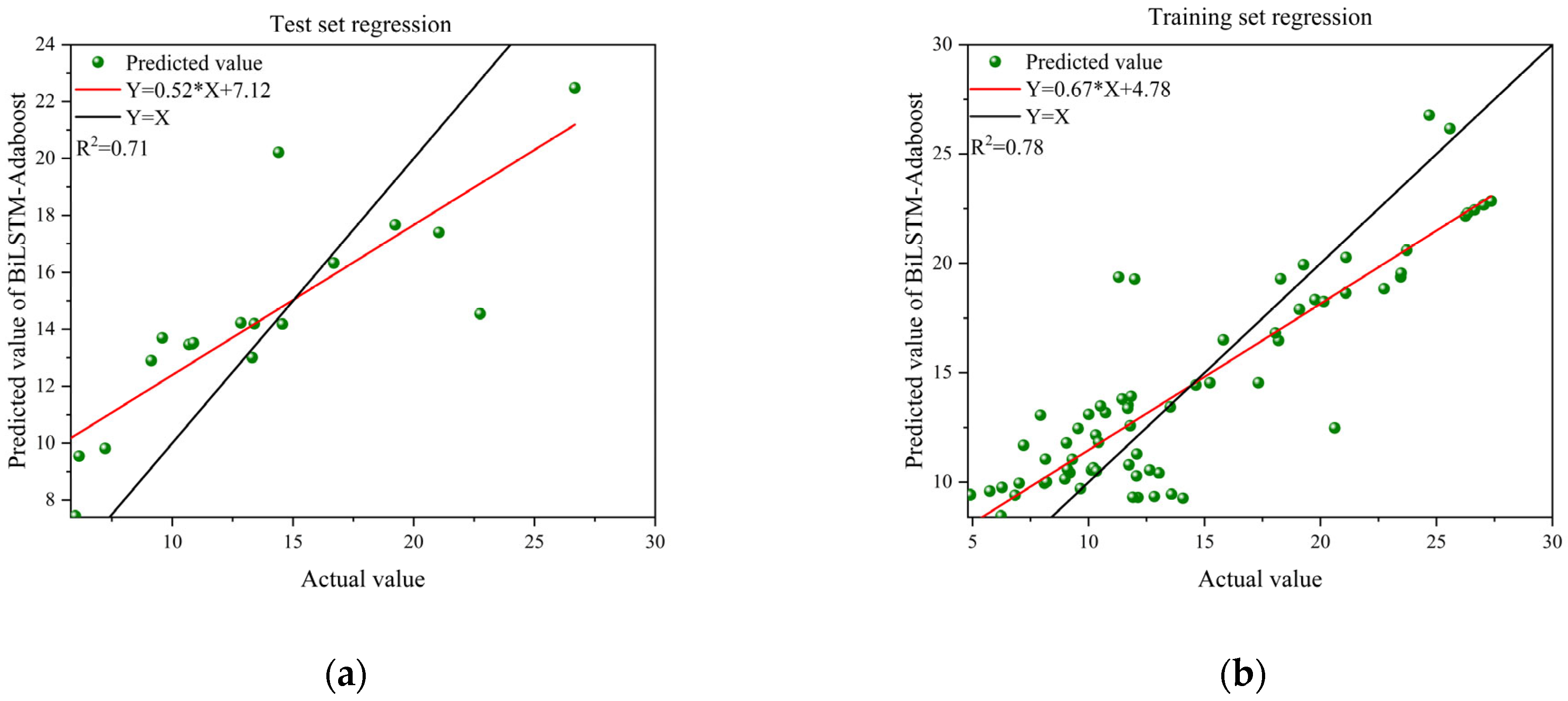
Figure 17 presents the linear fitting results of the BiLSTM-Adaboost model. It is evident that the BiLSTM-Adaboost model performs better than the CNN model, with an R2 value of 0.7664. The fitting curve approaches the ideal 45-degree line, demonstrating higher accuracy and robustness in handling complex time-series data.
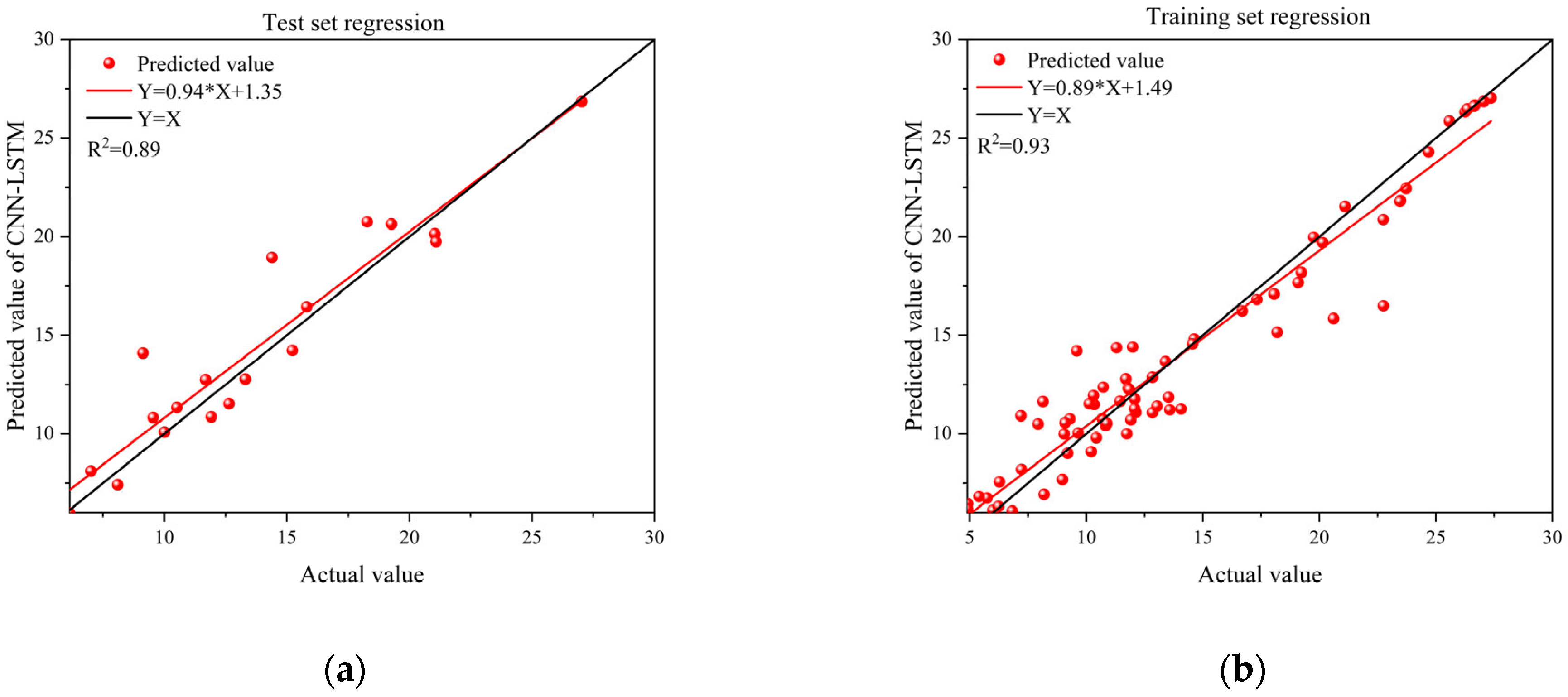
Figure 18 shows the linear fitting results of the CNN-LSTM model. Compared to previous models, the LSTM model performs well in capturing temporal dependencies, with an R2 value of 0.8828. This indicates a significant improvement in data fitting, although some high-pressure data points still deviate from the ideal curve, leaving room for minor errors.
Figure 19 illustrates the linear fitting results of the CNN-BiLSTM model. The figure shows that the CNN-BiLSTM model fits the data well, with the fitting curve close to the ideal 45-degree line. The R2 value of the CNN-BiLSTM model is 0.9425, demonstrating excellent performance in handling time-series data and significantly better fitting accuracy compared to previous models.
Figure 20 presents the linear fitting results of the CNN-BiLSTM-Adaboost model. Compared to other models, the fitting curve of the CNN-BiLSTM-Adaboost model is the closest to the ideal 45-degree line, with an R2 value of 0.9532, the highest among all models. This indicates that this model has the strongest fitting ability and prediction accuracy in pipeline residual strength prediction, further validating its effectiveness as the optimal model.
Figure 21 presents the linear fitting results of the CNN-BiLSTM-XGBoost model. Compared to other models, the CNN-BiLSTM-XGBoost model achieves a moderate alignment with the ideal 45-degree line, with an R2 value of 0.7205. Although the fitting curve shows noticeable deviations in certain regions, the overall trend suggests that the model can effectively learn key patterns in the data. The integration of CNN for spatial feature extraction, BiLSTM for capturing temporal dependencies, and XGBoost for enhanced nonlinear learning contributes to its balanced performance. While its predictive accuracy is not as high as the top-performing models, it demonstrates promising potential for improvement and serves as a competitive alternative in pipeline residual strength prediction.
The prediction results and the calculated average relative errors from the four optimization models visually demonstrate that among the bioinspired algorithms, the model optimized using the CNN-BiLSTM-Adaboost parameters performs the best. The CNN-BiLSTM-Adaboost algorithm shows an average relative error of 4.6944% and has 1 point not satisfying conservatism out of the 20 predicted pipeline residual strength influencing factor data. Among exhaustive search optimization algorithms, the CNN-BiLSTM algorithm has four points not satisfying conservatism, and its average relative error is relatively higher compared to the CNN-BiLSTM-Adaboost algorithm, leading to a slight deficiency in accuracy. Therefore, the CNN-BiLSTM-Adaboost algorithm is chosen as the optimal model for predicting the residual strength of pipelines with corrosion defects. The predicted results are then compared with the standard evaluation methods.

3.2. Comparison of CNN-BiLSTM-Adaboost Algorithm and Standard Methods for Residual Strength Prediction

For commonly used standard methods for pipeline residual strength evaluation, the American Society of Mechanical Engineers (ASME) B31G evaluation method, Det Norske Veritas Recommended Practice (DNV RP)-F101 evaluation method, and Pipeline Coatings and Corrosion Research Council (PCORRC) evaluation method are representative. To feasibly study the CNN-BiLSTM-Adaboost-based pipeline residual strength evaluation method, the predicted results of the CNN-BiLSTM-Adaboost algorithm are compared with the evaluation results of ASME B31G, DNV RP-F101, and PCORRC for the 20 predicted samples and the actual residual strength of the pipeline. The average relative error and conservatism situations for the 20 sets of data are calculated and presented in Table 5.
It is observed that, among the CNN-BiLSTM-AdaBoost algorithm, ASME B31G evaluation method, DNV RP F101 evaluation method, and PCORRC evaluation method, the CNN-BiLSTM-AdaBoost algorithm has a relatively smaller average relative error in the evaluation results. Compared with the traditional ASME B31G, DNV RP F101, and PCORRC standards, CNN-BiLSTM-AdaBoost method reduces the average relative error by 28.901%, 43.391%, and 40.753%, respectively [40]. In terms of accuracy, the CNN–BiLSTM–AdaBoost algorithm outperforms the other three evaluation methods. However, in terms of conservatism, the CNN–BiLSTM–AdaBoost algorithm is not as conservative as traditional standard evaluation methods. In practical operations, to ensure the safe operation of pipelines, operators will not adjust the working pressure of the pipeline to the maximum working pressure but will reduce it to a certain pressure level as the actual working pressure of the pipeline. Although one data point in the CNN-BiLSTM-Adaboost algorithm’s predictions does not meet the conservative requirements of the pipeline, the overall impact on the safe operation of the pipeline is not fundamental. Moreover, the CNN-BiLSTM-Adaboost algorithm has higher accuracy. Therefore, the prediction results of the CNN-BiLSTM-Adaboost algorithm are more feasible and convenient compared to traditional evaluation methods.

4. Conclusions

In this study, we proposed a pipeline residual strength prediction model based on the CNN-BiLSTM-Adaboost algorithm and verified its effectiveness and feasibility in practical applications. Through correlation analysis, we explored the relationships between pipeline wall thickness, defect depth, defect length, and burst pressure. Based on these findings, the prediction capability of the model was enhanced by combining CNN, BiLSTM, and AdaBoost algorithms. The results demonstrate that the proposed CNN-BiLSTM-AdaBoost model achieves an average relative error of only 4.694%, with just one non-conservative point, significantly outperforming traditional methods. Specifically, compared to the ASME B31G, DNV RP F101, and PCORRC methods—which exhibit average relative errors of 33.595%, 48.085%, and 45.447%, respectively—our model reduces the predictive error by 28.901%, 43.391%, and 40.753%, respectively. Therefore, the CNN-BiLSTM-Adaboost model not only achieves high prediction accuracy but also demonstrates good conservatism and robustness, confirming its feasibility and superiority in pipeline residual strength prediction.

Author Contributions

Q.L.: Methodology, Writing—original draft, Software, Validation, Formal analysis, Visualization. Y.W.: Resources, Supervision, Project administration, Writing—review and editing, Financial support. C.G.: Resources, Software, Investigation, Writing—review and editing. Y.G.: Resources, Supervision, Project administration. J.Y.: Resources, Supervision, Project administration. H.X.: Supervision, Financial support. Z.Y.: Supervision, Financial support. All authors have read and agreed to the published version of the manuscript.

Funding

This research was funded by the Basic Science (Natural Science) Research General Projects in Higher Education Institutions of Jiangsu Province (No. 23KJB130007), the Major Project of Fundamental Research on Frontier Leading Technology of Jiangsu Province (NO. BK20222006), the Double Innovation Doctor of Jiangsu Province (No. JSSCBS20220698), the National Natural Science Foundation of China (No. 52278505, No. 62303272), the Jiangsu Province Innovation Support Program (No. BZ2022037), the Nanjing Forestry University College Student Innovation Training Program (No.2024NFUSPITP0043), the Postdoctoral Innovation Project of Shandong Province (SDCX-ZG-202203036), and the Natural Science Foundation of Shandong Province (ZR2021QF135, ZR2022QF038).

Institutional Review Board Statement

This article does not contain any studies with human participants or animals performed by any of the authors.

Informed Consent Statement

Not applicable.

Data Availability Statement

The data that support the findings of this study are available from the corresponding author [Yina Wang] upon reasonable request.

Conflicts of Interest

The authors declare that they have no known competing financial interests or personal relationships.

References

  1. Oh, D.; Race, J.; Oterkus, S.; Koo, B. Burst pressure prediction of API 5L X-grade dented pipelines using deep neural network. J. Mar. Sci. Eng. 2020, 8, 766. [Google Scholar] [CrossRef]
  2. Lu, H.; Iseley, T.; Matthews, J.; Liao, W.; Azimi, M. An ensemble model based on relevance vector machine and multi-objective SALP swarm algorithm for predicting burst pressure of corroded pipelines. J. Pet. Sci. Eng. 2021, 203, 108585. [Google Scholar] [CrossRef]
  3. Lu, H.; Xu, Z.D.; Iseley, T.; Matthews, J.C. Novel data-driven framework for predicting residual strength of corroded pipelines. J. Pipeline Syst. Eng. Pract. 2021, 12, 04021045. [Google Scholar] [CrossRef]
  4. Ma, Y.; Zheng, J.; Liang, Y.; Klemeš, J.J.; Du, J.; Liao, Q.; Lu, H.; Wang, B. Deep pipe: Theory-guided neural network method for predicting burst pressure of corroded pipelines. Process Saf. Environ. Prot. 2022, 162, 595–609. [Google Scholar] [CrossRef]
  5. Lu, H.; Peng, H.; Xu, Z.D.; Matthews, J.C.; Wang, N.; Iseley, T. A feature selection-based intelligent framework for predicting maximum depth of corroded pipeline defects. J. Perform. Constr. Facil. 2022, 36, 04022044. [Google Scholar] [CrossRef]
  6. Kong, X.; Wang, Z.; Xiao, F.; Bai, L. Power load forecasting method based on demand response deviation correction. Int. J. Electr. Power Energy Syst. 2023, 148, 109013. [Google Scholar] [CrossRef]
  7. Chen, Z.; Li, X.; Wang, W.; Li, Y.; Shi, L.; Li, Y. Residual strength prediction of corroded pipelines using multilayer perceptron and modified feed-forward neural network. Reliab. Eng. Syst. Saf. 2023, 231, 108980. [Google Scholar] [CrossRef]
  8. Sulaiman, S.M.; Jeyanthy, P.A.; Devaraj, D.; Shihabudheen, K.V. A novel hybrid short-term electricity forecasting technique for residential loads using empirical mode decomposition and extreme learning machines. Comput. Electr. Eng. 2022, 98, 107663. [Google Scholar] [CrossRef]
  9. Yan, S.R.; Tian, M.; Alattas, K.A.; Mohamadzadeh, A.; Sabzalian, M.H.; Mosavi, A.H. An experimental machine learning approach for midterm energy demand forecasting. IEEE Access 2022, 10, 118926–118940. [Google Scholar] [CrossRef]
  10. Zhao, D.; Wang, T.; Chu, F. Deep convolutional neural network based planet bearing fault classification. Comput. Ind. 2019, 107, 59–66. [Google Scholar] [CrossRef]
  11. Chuang, W.Y.; Tsai, Y.L.; Wang, L.H. Leak detection in water distribution pipes based on CNN with mel frequency cepstral coefficients. In Proceedings of the 3rd International Conference on Innovative Artificial Intelligence, Suzhou, China, 15–18 March 2019. [Google Scholar]
  12. Zhou, M.; Yang, Y.; Xu, Y.; Hu, Y.; Cai, Y.; Lin, J.; Pan, H. A pipeline leak detection and localization approach based on ensemble TL1DCNN. IEEE Access 2021, 9, 47565–47578. [Google Scholar] [CrossRef]
  13. Kang, J.; Park, Y.-J.; Lee, J.; Wang, S.-H.; Eom, D.-S. Novel leakage detection by ensemble CNN-SVM and graph-based localization in water distribution systems. IEEE Trans. Ind. Electron. 2017, 65, 4279–4289. [Google Scholar] [CrossRef]
  14. Ratinov, L.; Roth, D. Design challenges and misconceptions in named entity recognition. In Proceedings of the 13th Conference on Computational Natural Language Learning, Boulder, CO, USA, 4 June 2009. [Google Scholar]
  15. Petasis, G.; Petridis, S.; Paliouras, G.; Karkaletsis, V.; Perantonis, S.J.; Spyropoulos, C.D. Symbolic and neural learning for named-entity recognition. In Proceedings of the Symposium on Computational Intelligence and Learning, Chios, Greece, 19–23 June 2000. [Google Scholar]
  16. Luo, G.; Huang, X.; Lin, C.Y.; Nie, Z.Q. Joint entity recognition and disambiguation. In Proceedings of the 2015 Conference on Empirical Methods in Natural Language Processing, Lisbon, Portugal, 17–21 September 2015. [Google Scholar]
  17. Cody, R.A.; Tolson, B.A.; Orchard, J. Detecting leaks in water distribution pipes using a deep autoencoder and hydroacoustic spectrograms. J. Comput. Civ. Eng. 2020, 34, 04020001. [Google Scholar] [CrossRef]
  18. Guo, G.; Yu, X.; Liu, S.; Ma, Z.; Wu, Y.; Xu, X.; Wang, X.; Smith, K.; Wu, X. Leakage detection in water distribution systems based on time-frequency convolutional neural network. J. Water Resour. Plan. Manag. 2021, 147, 04020101. [Google Scholar] [CrossRef]
  19. Santos, C.; Guimaraes, V.; Niteroi, R.J.; Rio, J. Boosting named entity recognition with neural character embeddings. In Proceedings of the 5th Named Entities Workshop, Beijing, China, 31 July 2015. [Google Scholar]
  20. Gers, F.A.; Schmidhuber, J.; Cummins, F. Learning to forget: Continual prediction with LSTM. Neural Comput. 2000, 12, 2451–2471. [Google Scholar] [CrossRef] [PubMed]
  21. Goller, C.; Kuchler, A. Learning task-dependent distributed representations by backpropagation through structure. In Proceedings of the IEEE International Conference on Neural Networks, Washington, DC, USA, 3–6 June 1996. [Google Scholar]
  22. Labeau, M.; Loser, K.; Allauzen, A. Non-lexical neural architecture for fine-grained POS tagging. In Proceedings of the 2015 Conference on Empirical Methods in Natural Language Processing, Lisbon, Portugal, 17–21 September 2015. [Google Scholar]
  23. Du, J.; Cheng, Y.; Zhou, Q.; Zhang, J.; Zhang, X. Power load forecasting using BiLSTM-attention. IOP Conf. Ser. Earth Environ. Sci. 2020, 440, 032115. [Google Scholar] [CrossRef]
  24. Chunsheng, C.; Mengqing, T.; Kejia, Z. Pipeline anomaly data detection method based on Bi-LSTM network. Comput. Technol. Dev. 2023, 33, 215–220. [Google Scholar]
  25. Li, H.; Wang, S.; Islam, M.; Bobobee, E.D.; Zou, C.; Fernandez, C. A novel state of charge estimation method of lithium-ion batteries based on the IWOA-AdaBoost-Elman algorithm. Int. J. Energy Res. 2021, 46, 5134–5151. [Google Scholar] [CrossRef]
  26. Fu, Y.; Zheng, Y.; Hao, S.; Miao, Y. Research on comprehensive decision-making of distribution automation equipment testing results based on entropy weight method combined with grey correlation analysis. J. Phys. Conf. Ser. 2021, 2005, 012033. [Google Scholar] [CrossRef]
  27. Durante, F.; Sempi, C. Principles of Copula Theory; CRC Press: Boca Raton, FL, USA, 2016. [Google Scholar]
  28. Zhengshan, L.; Jiaqi, Z.; Jihao, L. Research on failure pressure prediction of corroded pipelines based on integrated algorithm. Comput. Technol. Dev. 2024, 34, 80–86. [Google Scholar]
  29. Bjornoy, O.H.; Rengard, O.; Fredheim, S. Residual strength of dented pipelines, DNV test results. In Proceedings of the 10th International Offshore and Polar Engineering Conference, Washington, DC, USA, 28 May–2 June 2000. [Google Scholar]
  30. Freire, J.L.F.; Vieira, R.D.; Castro, J.T.P.; Benjamin, A.C. PART 3: Burst tests of pipeline with extensive longitudinal metal loss. Exp. Tech. 2006, 30, 60–65. [Google Scholar] [CrossRef]
  31. Wang, S.H.; Fernandes, S.L.; Zhu, Z.; Zhang, Y.D. AVNC: Attention-Based VGG-Style Network for COVID-19 Diagnosis by CBAM. IEEE Sens. J. 2022, 22, 17431–17438. [Google Scholar] [CrossRef] [PubMed]
  32. Qin, L.; Yu, N.; Zhao, D. Applying the convolutional neural network deep learning technology to behavioural recognition in intelligent video. Teh. Vjesn. Tech. Gaz. 2018, 25, 528–535. [Google Scholar]
  33. Hao, Y.; Gao, Q. Predicting the trend of stock market index using the hybrid neural network based on multiple time scale feature learning. Appl. Sci. 2020, 10, 3961–3974. [Google Scholar] [CrossRef]
  34. Kamalov, F. Forecasting significant stock price changes using neural networks. Neural Comput. Appl. 2020, Early Access. [Google Scholar] [CrossRef]
  35. Fanta, H.; Shao, Z.; Ma, L. ‘Forget’ the Forget Gate: Estimating Anomalies in Videos using Self-contained Long Short-Term Memory Networks. In Proceedings of the International Conference on Artificial Intelligence and Soft Computing, Geneva, Switzerland, 20–23 October 2020. [Google Scholar]
  36. Siami-Namini, S.; Tavakoli, N.; Namin, A.S. The Performance of LSTM and BiLSTM in Forecasting Time Series. In Proceedings of the IEEE International Conference on Big Data, Los Angeles, CA, USA, 9–12 December 2019. [Google Scholar]
  37. Quan, R.; Zhu, L.; Wu, Y.; Yang, Y. Holistic LSTM for Pedestrian Trajectory Prediction. IEEE Trans. Image Process. 2021, 30, 1–12. [Google Scholar] [CrossRef]
  38. Pu, W. Analysis of ASME B31G residual strength evaluation method. Chem. Des. Commun. 2019, 45, 140–141. [Google Scholar]
  39. Det Norske Veritas. DNV RP-F101-1999 Recommended Practice for Corroded Pipeline; DNV: Oslo, Norway, 1999. [Google Scholar]
  40. Xiao, G.; Feng, M.; Zhang, H.; Chen, J.; Wang, F.; Yu, H. Study on failure assessment of X80 high-grade pipeline with defect corrosion. China Saf. Sci. Technol. 2015, 6, 128–133. [Google Scholar]
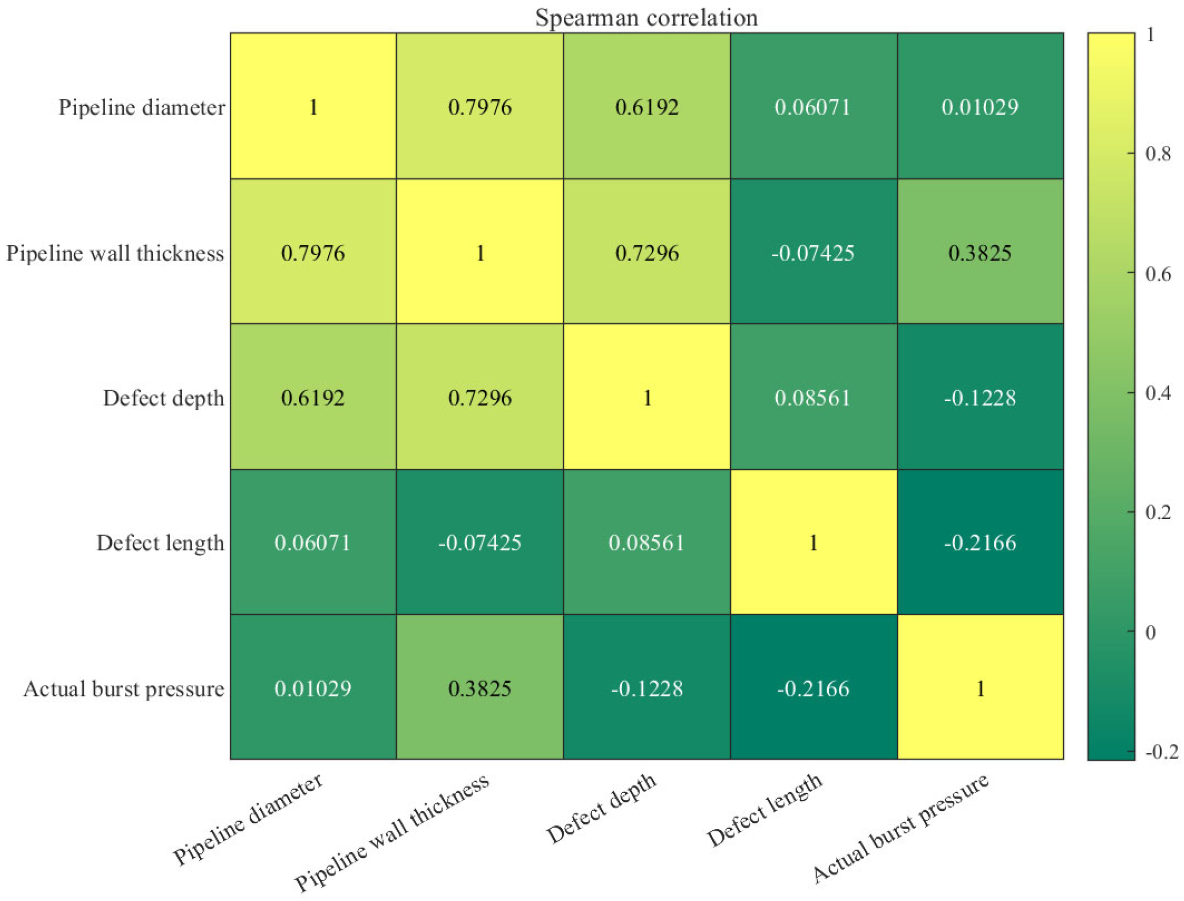
Figure 1. Correlation analysis result graph.
Applsci 15 09059 g001
Figure 2. Strategy diagram of prediction method.
Applsci 15 09059 g002
Figure 3. The basic structure of CNN.
Applsci 15 09059 g003
Figure 4. The basic structure of LSTM.
Applsci 15 09059 g004
Figure 5. The basic structure of BiLSTM.
Applsci 15 09059 g005
Figure 6. CNN-BiLSTM model structure diagram.
Applsci 15 09059 g006
Figure 8. Activity diagram of CNN-BiLSTM-Adaboost training process.
Applsci 15 09059 g008
Figure 10. Prediction results graph of the CNN model.
Applsci 15 09059 g010
Figure 11. Prediction results graph of the BiLSTM-Adaboost model.
Applsci 15 09059 g011
Figure 12. Prediction results graph of the CNN-LSTM model.
Applsci 15 09059 g012
Figure 13. Prediction results graph of the CNN-BiLSTM model.
Applsci 15 09059 g013
Figure 14. Prediction results graph of the CNN-BiLSTM-Adaboost model.
Applsci 15 09059 g014
Figure 15. Prediction results graph of the CNN-BiLSTM-XGBoost model.
Applsci 15 09059 g015
Figure 16. CNN prediction results in linear fitting graph.
Applsci 15 09059 g016
Figure 17. BiLSTM-Adaboost prediction results in linear fitting graph.
Applsci 15 09059 g017
Figure 18. CNN-LSTM prediction results in linear fitting graph.
Applsci 15 09059 g018
Figure 19. CNN-BiLSTM prediction results in linear fitting graph.
Applsci 15 09059 g019
Figure 20. CNN-BiLSTM-Adaboost prediction results in linear fitting graph.
Applsci 15 09059 g020
Figure 21. CNN-BiLSTM-XGBoost prediction results in linear fitting graph.
Applsci 15 09059 g021
Table 1. Pipeline data source.
Pipeline Steel Grade (mm)Data Sources
X35reference literature [28]
X42reference literature [29,30]
X46reference literature [28,29,30,31]
X52reference literature [31,32]
X56reference literature [32]
X60reference literature [29,31]
X65reference literature [28,29,32]
X80reference literature [32]
X100reference literature [32]
Table 2. Partial pipeline blasting data.
Serial NumberPipeline Steel GradePipeline Inner Diameter (mm)Pipeline Wall Thickness (mm)Defect Depth (mm)Defect Length (mm)Burst Pressure (MPa)
1X3550873.3304.812
2X4252994.716015.7
3X46457.76.236.23275012.06
4X52273.055.231.85408.9416.71
5X56506.735.743.02132.0810.73
6X6050814.310.0350013.4
7X6576217.54.420024.11
8X80121919.891.77607.7423.3
Table 3. Parameters’ setting of CNN-BiLSTM method.
ParametersValue
Convolution layer filters64
Convolution layer kernel size1
Convolution layer activation functionRELU
Convolution layer paddingSame
Pooling layer pool size1
Pooling layer paddingSame
Pooling layer activation functionRELU
Number of hidden units in BiLSTM layer64
Table 4. CNN model prediction results relative error and conservative point situation.
Algorithm R M S E M A E M A P E   ( % ) R 2
CNN4.39633.279428.80840.6354
LSTM8.54707.14753.7685−5.5987
BiLSTM6.31175.595835.4587−2.9485
BiLSTM-Adaboost3.06542.528915.09260.7664
CNN-LSTM1.85161.32918.18820.8828
CNN-BiLSTM1.96191.17575.98470.9425
CNN-BiLSTM-XGBoost3.38282.311925.07960.7205
CNN-BiLSTM-Adaboost1.57321.24634.69440.9532
Table 5. The relative error and conservatism of prediction results of intelligent algorithm and standard method model.
Evaluation MethodsCNN-BiLSTM-AdaboostASME B31GDNV RP-F101PCORRC
average relative error (%)4.69433.59548.08545.447
number of points not meeting conservatism1244
Disclaimer/Publisher’s Note: The statements, opinions and data contained in all publications are solely those of the individual author(s) and contributor(s) and not of MDPI and/or the editor(s). MDPI and/or the editor(s) disclaim responsibility for any injury to people or property resulting from any ideas, methods, instructions or products referred to in the content.