Abstract
Automated threat detection in X-ray security imagery is a critical yet challenging task, where conventional deep learning models often struggle with low accuracy and overfitting. This study addresses these limitations by introducing a novel framework based on feature fusion. The proposed method extracts features from multiple and diverse deep learning architectures and classifies them using a Random Weight Network (RWN), whose hyperparameters are optimized for maximum performance. The results show substantial improvements at each stage: while the best standalone deep learning model achieved a test accuracy of 83.55%, applying the RWN to a single feature set increased accuracy to 94.82%. Notably, the proposed feature fusion framework achieved a state-of-the-art test accuracy of 97.44%. These findings demonstrate that a modular approach combining multi-model feature fusion with an efficient classifier is a highly effective strategy for improving the accuracy and generalization capability of automated threat detection systems.
1. Introduction
The integrity of security screening in public spaces, such as airports, is a critical component of both national and international safety. Although numerous security measures are implemented, systems reliant on human operators remain vulnerable to error, potentially leading to severe security breaches with significant material and societal consequences. X-ray imaging systems play a central role in these security protocols, particularly for baggage inspection. However, the manual identification of concealed threats within complex environments, such as improvised explosive circuits hidden inside electronic devices like laptops, presents a formidable challenge. This specific task requires a high level of specialized expertise and is inherently prone to human oversight, thereby creating a significant vulnerability in security checkpoints.
In response to these challenges, automated detection systems driven by deep learning have been explored by researchers. However, early investigations that applied conventional deep learning models directly to this problem revealed significant limitations. These limitations include relatively low classification accuracy and a high tendency towards overfitting, largely attributed to the complexity and inherent variations within the X-ray dataset [1]. The overlapping nature of components in X-ray images increases intra-class variation, while the visual similarity between benign laptop circuits and threat items elevates inter-class confusion, making robust classification difficult. To overcome these deficiencies, this study proposes a novel framework centered on feature fusion combined with a Random Weight Network (RWN) for classification. The core hypothesis is that features extracted from multiple and diverse deep learning architectures can provide a richer, more discriminative representation of the input data. By fusing these features and employing an RWN, which is noted for its rapid training and resistance to overfitting, it is anticipated that a more accurate and generalizable classification model can be achieved. This approach addresses the key research questions regarding the performance enhancement that can be achieved through feature fusion and the optimal configuration of the RWN classifier, including the impact of hidden neuron count and activation function.
The main contributions of this work are systematically outlined as follows:
- (a)
- A Novel Feature Fusion Framework: This study proposes and validates a new framework that integrates features extracted from multiple deep learning models (e.g., ShuffleNet, InceptionV3) and employs a Random Weight Network (RWN) for classification. This multi-source feature fusion strategy marks a significant departure from conventional single-model approaches.
- (b)
- Significant Performance Improvement: A substantial improvement in classification performance is demonstrated. The proposed feature fusion methodology achieves a test accuracy of 97.44%. This result is markedly superior to both the 83.55% accuracy of the best-performing individual deep learning model, ShuffleNet, and the 94.82% accuracy from classification using features from a single model with an optimized RWN.
- (c)
- Comprehensive Empirical Analysis: A comprehensive empirical analysis of the RWN-based classifier is conducted. The investigation evaluates the influence of critical hyperparameters, including the number of hidden neurons and the choice of activation functions, providing a clear optimization guide for similar security applications.
- (d)
- Robustness and Generalization: The robustness and generalization capability of the proposed method are established through a comparative analysis against 11 state-of-the-art machine learning classifiers. The framework is shown to offer superior generalization and effective mitigation of overfitting.
- (e)
- Publicly Available Dataset: A challenging new dataset of X-ray images, featuring laptops with and without concealed circuits, has been created and made publicly available [1], thereby providing a valuable benchmark for future research in this domain.
Within this framework, the following research questions are posed to articulate the study’s core contributions and key capabilities:
- (a)
- How does it affect the classification performance using RWN on datasets whose features are extracted by deep learning models?
- (b)
- Can the combination of features extracted from different deep learning models significantly improve training and test accuracy in classification?
- (c)
- What are the performance implications of existing deep learning algorithms when applied to X-ray security datasets, and how can these be addressed through feature fusion techniques?
- (d)
- How does the use of an RWN influence classification performance when compared to standard deep learning models on X-ray datasets?
- (e)
- Do the combinations of merged features (e.g., N|M and M|N) have a significant effect on classification outcomes in RWN?
- (f)
- What is the impact of the number of hidden layer neurons on the performance of an RWN, and how can the risk of overfitting be minimized through optimal parameter selection?
- (g)
- How does the selection of activation functions (sigmoid, tangent sigmoid, or hardlim) affect the classification performance of an RWN, particularly in the context of combined datasets?
The organization of the study is as follows: In Section 1, an introduction to the study is provided, a literature review is presented, and the motivation and contribution of the study are outlined. Section 2 covers feature extraction from deep learning models, feature fusion, and dataset explanation. In Section 3, experiments are conducted, and the results obtained are analyzed. Section 4 discusses the findings, and the study is finally concluded in Section 5.
X-ray imaging technologies have been used in various aspects of daily life, as well as in fields such as crystallography, astronomy, and medicine, since the discovery of X-rays by Wilhelm Conrad Rontgen. These technologies encompass a wide range of purposes and methods, including traditional transmission methods, dual-energy techniques, and scattered X-ray methods [2]. In these technologies, rays emitted from an X-ray source are attenuated as they pass through objects. This decrease in intensity is utilized to calculate the density (d) and effective atomic number (Zeff) of the materials [3]. Consequently, materials with higher density, which cause greater attenuation, appear brighter in X-ray images, while lower-density materials appear darker. X-ray technologies are widely used for various purposes, as evidenced by the information provided by X-ray devices. Applications range from inspecting welds in industrial settings and identifying bone fractures in medicine to detecting prohibited materials in security-sensitive locations like airports, courthouses, and shopping malls.
X-ray images are utilized for the detection of prohibited materials, aiming to minimize security risks at airports through the application of machine learning and image processing techniques. This involves identifying items passengers are forbidden to carry, whether on their person or in their luggage, by analyzing 3D or 2D X-ray images [4]. These applications are typically employed to assist personnel conducting baggage control or to automate the process. This section reviews the literature on X-ray image analysis and feature fusion using deep learning algorithms.
Previously, tasks such as classification in X-ray imaging were performed using manually extracted features, such as SIFT and PHOW, often within a Bag of Words (BoW) framework [5].
In later periods, the success of convolutional neural network (CNN) techniques led to their increased use in this field as well. Akçay et al. [6] implemented transfer learning in CNN using the fine-tuning paradigm. Jaccard et al. [7] detected the presence of threat materials in cargo containers using CNN on image patches. Mery et al. [8] compared methods such as Bag of Words, Sparse Representations, deep learning, and classical pattern recognition schemes. Jaccard et al. [9] also detected cars within cargo using CNN with data augmentation. Rogers et al. [10] used the original dual-energy images as separate channels in their CNN. They performed data augmentation with Threat Image Projection. Caldwell et al. [11], investigated transfer learning in different scenarios using deep networks, such as VGG. Morris et al. [12] focused on threat detection of traditional explosives using CNNs like VGG and Inception. In addition to these, newly emerged CNN models such as region-based CNNs [13] and single-shot models like YOLO (You Look Only Once) [14] have also been applied in X-ray imaging. Petrozziello and Jordanov [15] performed the detection of steel barrel holes using CNN and Stacked Autoencoder. Cheng et al. [16] used a YOLO-based method they called X-YOLO, which has feature fusion and attention mechanisms. Wu and Xu [17] used a hybrid Self-Supervised Learning in the pre-training phase to perform detection with a structure containing a transformer in the final stage of the Head-Tail Feature Pyramid head. Wang et al. [18] used a Yolov8-based method with a dual branch structure that includes Sobel convolution and convolution branches. Additionally, in the fusion part, they used a lightweight star operation module. In addition to classification, deep learning methods have also been employed for data augmentation. Yang et al. [19] performed data augmentation using generative adversarial networks (GANs), which utilize Fréchet Inception Distance scores and compared them (DCGAN, WGAN-GP). Kaminetzky and Mery [20] performed data augmentation using simulated 3D X-ray image models. Apart from these tasks, CNNs have also been used as feature extractors. Caldwell and Griffin [21] performed data augmentation with photographic images, using both photographs and X-ray images of the same object. Benedykciuk et al. [22] addressed the material recognition problem using a multiscale network structure consisting of five subnetworks and using image patches. Babalik and Babadag [23] used CNNs as feature extractors; in the next stages, they selected the features with a binary Sparrow Search Algorithm and classified them using Support Vector Machines (SVM) and k-nearest neighbors (KNN) as classifiers. Methods such as ensemble learning and feature fusion have also been used to improve the performance of deep learning models. Ayantayo et al. [24] proposed three different deep learning models, which used early-fusion, late-fusion, and late-ensemble learning strategies to resist overfitting. Zhang et al. [25] used multi-domain features, employing transfer learning and feature fusion. They used SVM in feature extraction and model selection stages, then fused these features and performed baby cry detection. Wu et al. [26] performed deep learning-based fault diagnosis for rolling bearings. In their method, they used a new multiscale feature fusion deep residual network containing multiple multiscale feature fusion blocks and a multiscale pooling layer. Liu et al. [27] implemented a multi-modal fusion approach that combines two different deep learning models trained on simple clinical information and group images, using logistic regression for breast nodule diagnosis. Patil and Kirange [28] proposed a method for detecting brain tumors by fusing deep network features, such as VGG Inception and a shallow CNN. Gill et al. [29] used deep learning methods including CNN, Recurrent Neural Network (RNN) and Long Short-Term Memory (LSTM) for image-based classification of fruits using early fusion and late fusion strategies. Deng et al. [30] addressed side-channel attacks in information security using feature extraction with a multi-scale feature fusion mechanism. Al-Timemy et al. [31] utilized Xception and InceptionResNetV2 deep learning architectures to extract features from three different corneal maps. The extracted features from these models were fused into one pool to train conventional machine learning classifiers. Peng and Zhang [32] presented a deep learning network based on multiple feature fusion as well as ensemble learning approaches for the diagnosis and treatment of lung diseases. A deep supervised ensemble learning network was used to combine multiple inducers to improve lung lobe segmentation. Tu et al. [33] proposed a general framework for solving online packing problems using deep reinforcement learning hyper-heuristics. They used feature fusion to combine the visual information of real-time packing with distributional information of random parameters of the problem. Tan et al. [34] performed component identification using a deep learning network based on coarse-grained feature fusion. Medjahed et al. [35] fused CNNs trained on different modalities using machine learning (ML) algorithms in the classification phase. Ma et al. [36] proposed a deep dual-side learning ensemble model for Parkinson’s disease diagnosis by analyzing speech data. Their approach employs a weighted fusion mechanism to integrate multiple models. Alzubaidi et al. [37] detected shoulder abnormalities. They trained models using different body part images in the same domain and performed feature fusion with different machine learning classifiers. Agarwal et al. [38] used an approach that combined channel-based fusion and model-based fusion to classify chest x-ray images using ResNet50V3 and InceptionV3 models. Li et al. [39] designed a dual-channel feature fusion network for detecting distal radius fractures. They used Faster region-based CNN (RCNN)and ResNet50 on their channels. The feature fusion method includes an attention mechanism.
While a broader overview of deep learning for X-ray analysis is available in the literature [40], the foundation for the current study is the authors' prior work [1]. That paper details the creation of the dataset used herein and presents a comparative performance analysis of 11 different deep learning models.
The dataset presented in [1] is highly challenging due to two primary factors. Firstly, the overlapping nature of internal components in X-ray images leads to high intra-class variation. Secondly, high inter-class similarity, resulting from the visual resemblance between benign laptop circuits and threat circuits, reduces the distinction between the classes. Collectively, these issues caused the models evaluated in the previous work [1] to be prone to overfitting, a problem exacerbated by the dataset's limited size and high complexity. To overcome this issue and improve classification performance, it was proposed to use the RWN network for the fusion of the feature extraction capabilities of the pre-trained models in a way that is resistant to overfitting. This was anticipated to increase fusion success due to both the single-stage nature of the training and its resistance to overfitting.
Therefore, the motivation for this study is twofold: to address the identified gap in the literature for this specific security application and to overcome the performance limitations of conventional deep learning models that were observed in our prior work [1].
2. Feature Extraction Using Deep Learning
The fundamental difference between deep learning architectures and classical artificial neural networks is their ability to extract features from raw data. This is particularly popular in image processing, analysis, and classification. One significant reason for this popularity is that each pixel can be considered as a feature, leading to millions of features depending on the image resolution. The primary purpose of convolution filters used in image analysis or classification is to extract a feature map. Typically, due to the high number of extracted features, there is a pooling layer following the filter layers. The general scheme of convolution filters is illustrated in Figure 1, and pooling is depicted in Figure 2.
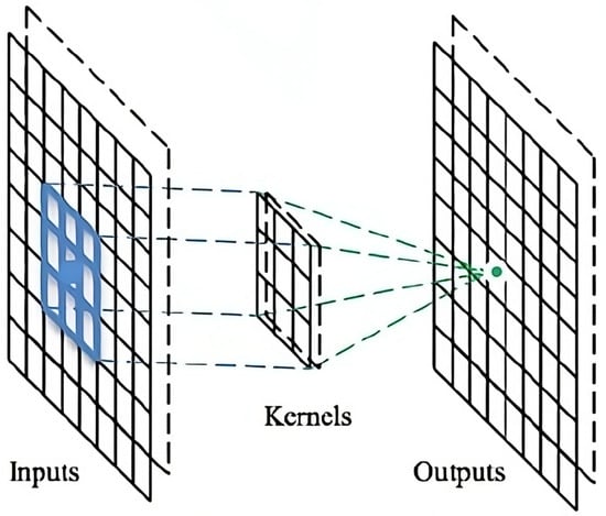
Figure 1.
The extraction of feature maps through filtering on an image.
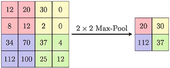
Figure 2.
2 × 2 Maximum pooling.
Different architectures have been proposed in the literature for various purposes, such as preventing the vanishing gradient problem by using a different number of convolution filters and pooling, improving the connectivity structure between layers, scalability, reducing computational costs, and achieving higher-performing models. In the scope of this study, ResNet, DarkNet, EfficientNet, DenseNet, MobileNet, InceptionV3, ShuffleNet, and Xception models were trained with the dataset, and features were extracted from these models. After obtaining the features, various machine learning methods such as kNN [41,42,43], SVM [42,43], and random forest [42,43] have been applied in the literature. In the scope of this study, feature vectors from 11 deep learning methods were obtained. An example of extracting and obtaining features after the training of the ResNet18 deep learning architecture is illustrated in Figure 3.
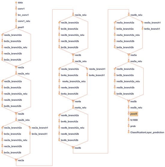
Figure 3.
ResNet model and the layer where features are extracted from the ResNet architecture.
After training, data are passed through the network, and features are extracted from the outputs of intermediate layers, such as convolutional or pooling layers, prior to the final fully connected layer. Table 1 summarizes the models used, the specific layers from which features are extracted, and the corresponding number of extracted features.

Table 1.
Layers from which features are extracted and the number of extracted features from deep learning models.
Table 1 Facilitates the comparison of different deep learning models based on the layers chosen for feature extraction and the dimensionality of the extracted features. The number of features reflects the complexity and expressive power of each model in capturing information from the input data.
2.1. Late Feature Fusion and Random Weight Network
After extracting N features from one deep learning method and M features from another, two datasets are obtained. These datasets, combined in the forms of (N | M) and (M | N), are subsequently used for training and classification. The overall process of feature extraction, merging, training, and testing is illustrated in Figure 4.
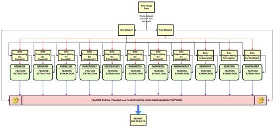
Figure 4.
The general diagram of feature extraction, fusion and classification in the study.
In Figure 4, after feature extraction, the RWN is employed for the training and testing process. For the training of an RWN, the network must have a three-layered structure consisting of an input layer, a hidden layer, and an output layer [44,45,46,47]. The structure of the RWN architecture is shown in Figure 5.
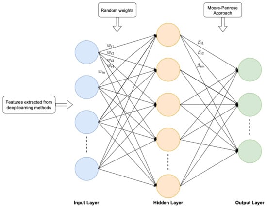
Figure 5.
A general architecture of Random Weight Networks.
In Figure 5, the features extracted from deep learning networks are provided to the input layer. The weights between the input layer and the hidden layer are randomly initialized. The Moore–Penrose approach is used between the hidden layer and the output layer. Unlike networks trained with iterative algorithms like backpropagation, an RWN calculates the output layer weights analytically in a single step. This non-iterative process results in significantly faster training time. In the current study, the RWN model and training algorithm proposed in [46,47] are used. In a feedforward artificial neural network with N neurons in the hidden layer and an activation function denoted as g(x), the output calculation for M training examples is performed using Equation (1).
where represents the input vector, is the target label vector, is the weight vector between the input and hidden layers, is the weight vector between the hidden and output layers and denotes the bias of the hidden neuron. By considering the explanations mentioned above, the model can be written as follows.
In Equation (2), is the output matrix of the hidden layer. To train the feedforward artificial neural network, specific weights and are calculated using a gradient-based learning algorithm as follows:
In the RWN, after the weights between the input layer and the hidden layer are randomly assigned, the weights () between the hidden layer and the output layer can be calculated as in Equation (4).
where, is the Moore–Penrose generalized inverse matrix. In an RWN, if the number of training examples equals the number of hidden neurons, the hidden layer output matrix H becomes a square matrix, and its direct inverse can be computed without the need for the Moore–Penrose approach. However, since the number of training examples is generally greater than the number of neurons in the hidden layer, the Moore–Penrose approach is used to compute the inverse of the matrix. The reason for the fast training process of an RWN is shown in Equation (4), while iterative methods are used to determine the weights given in Equation (3). In the current study, the classification` performance of the RWN was measured using the accuracy value, which represents the ratio of correctly predicted samples by the model.
2.2. Dataset
The study focuses on the development of deep learning methods for the detection of concealed circuits within laptops and emphasizes feature fusion. In this context, there is a need for a dataset to train, test, and extract features from deep learning methods. To meet this requirement, a multi-step process was followed to generate the dataset. This process involved the following:
- Creating the circuits and/or elements to be concealed;
- Procuring a variety of laptops;
- Capturing X-ray images of the circuits after they were hidden inside the laptops.
Readily available Arduino boards were chosen as the example circuits for concealment. Due to the high prices of new laptops and the need for many different laptops, second-hand laptops were purchased from the market. With permission obtained from the Konya Airport Civil Administration Directorate, X-ray images of 60 laptops with different configurations were obtained using X-ray devices at the airport. X-ray images of laptops taken from different angles are provided in Figure 6. In Figure 6, the areas enclosed in red rectangles contain hidden circuits not belonging to the computer motherboard, and the rectangles are drawn manually.
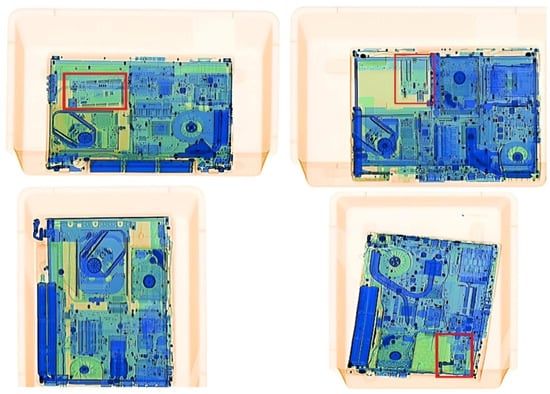
Figure 6.
X-ray images of laptops obtained from different angles.
As seen in Figure 6, the image of the laptop's motherboard and the embedded circuit is enclosed in a plastic box (standard practice at airports). Since the plastic transport box is irrelevant for classification, its image was removed from the background using a thresholding technique. This process also eliminated the bright yellow artifacts present in the images. In Figure 7, a clean X-ray image of the laptop is presented.
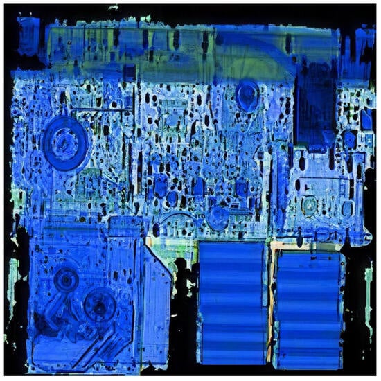
Figure 7.
Cleaned and segmented X-ray image.
A total of 6395 X-ray images were captured. Among them, 2545 contain hidden circuits, while 3850 do not. To ensure balance in the data, the number of images without circuits was reduced to 2549, and a total of 5094 X-ray images were used in the experiments. Since the problem is treated as a classification problem, labels for the images are necessary during the training and testing processes with deep learning methods. The 5094 X-ray images were marked as normal or abnormal and stored in different folders. Due to variations in input dimensions in the literature analysis and the deep learning architectures used, the images were resized for each deep learning algorithm to match the input size. Although the width of the conveyor belt of the X-ray machine (number of columns in the image) is expressed as 704 pixels, the length varies due to the continuous flow behavior of the belt (this is not clearly seen in Figure 6 due to its white background). Therefore, as shown in Figure 7, the background and object images were segmented, and a clean image was obtained. This image was then adapted to fit the input of each deep learning method.
3. Experiments
All experiments were conducted on a workstation equipped with an AMD Ryzen 9 5950X 16-Core Processor and 64 GB of RAM. The MATLAB 2021a environment was used for all stages of the study, including feature extraction, feature fusion, and the training and evaluation of the classification models.
The feature extraction process requires deep learning models to first be trained on the dataset. A comprehensive performance analysis of 11 such architectures was previously presented in [1]. The results from that study showed that ShuffleNet achieved the highest test accuracy of 83.55%, followed by the InceptionV3 architecture at 81.31%. In this study, the aim was to achieve higher accuracy in classification using features extracted from these architectures. The number of features extracted from the methods in the [1] study is presented in Table 2.
Table 2.
The number of extracted features using deep learning models.
The features for the datasets obtained by combining the features given in Table 2 are provided in Table 3.
Table 3.
The number of combined features obtained from deep learning models.
As seen in Table 3, besides using features from different architectures, the feature set from each architecture was concatenated with itself to investigate the effect of this repetition on classification performance. The datasets were used to conduct classification experiments with RWN, employing 10-fold cross-validation in each experiment. To account for the stochastic nature of the RWN, where input-to-hidden layer weights are randomly assigned, we repeated each 10-fold cross-validation experiment 30 times to obtain statistically robust performance measures. Our investigation focused on two key hyperparameters that govern RWN's behavior: the number of hidden layer neurons and the choice of activation function. The investigation began by evaluating the impact of the number of hidden neurons, testing the values as follows: 50, 100, 250, 500, 1000, 2000, and 4585. The value of 4585 was specifically chosen because it matches the number of training samples in each fold of our 10-fold cross-validation. When the number of hidden neurons equals the number of training samples, the hidden layer output matrix (H) becomes a square matrix, allowing its inverse to be calculated directly without requiring the Moore–Penrose pseudo-inverse method. Subsequently, the effect of the activation function, the second key hyperparameter, was investigated. For these experiments, the number of hidden neurons was fixed to the value that yielded the best average test accuracy from the previous stage. The activation functions evaluated include tangent sigmoid, sigmoid, sine, hard limit, triangular basis, and radial basis, all of which are commonly used with RWNs.
Firstly, the features given in Table 2 were reclassified using RWN and compared with the results of deep learning methods. Tangent sigmoid was used as the activation function in RWN, and the comparison results are presented in Table 4.
Table 4.
The comparison of deep learning models and RWN with different numbers of neurons in the hidden layer on the dataset.
Table 4 reveals a substantial improvement in test accuracy when features extracted from deep learning models are classified using an RWN. Specifically, while the best-performing standalone deep learning model (ShuffleNet) achieved an accuracy of 83.55%, this figure increased to 94.82% when using an RWN with 250 hidden neurons on the features extracted from the same ShuffleNet model. Additionally, the results indicate a trade-off related to the number of hidden neurons: increasing the neuron count improves training accuracy at the cost of decreasing test accuracy. This trend, which is indicative of overfitting, is illustrated for several model architectures in Figure 8.
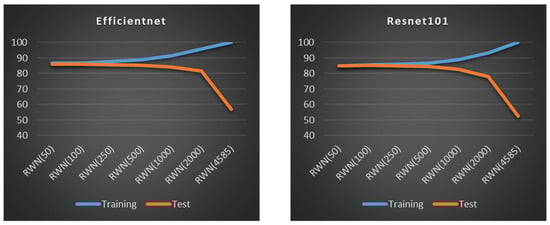
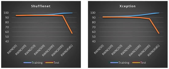
Figure 8.
The effect of the number of neurons in the RWN hidden layer on training and test accuracy.
A similar analysis using classical machine learning algorithms shows that features extracted from ShuffleNet consistently yield the best performance. Both SVM and KNN demonstrated strong generalization, achieving test accuracies of 93.62% and 94.76%, respectively, on the ShuffleNet features, results that are comparable to those of the RWN. In contrast, while the TREE model achieved high accuracy on the training set, its performance dropped significantly on the test set, clearly emphasizing its tendency to overfit. This comparison highlights the superior generalization capabilities of RWN, SVM, and KNN for this classification task.
A combined evaluation of Table 4 and Figure 8 indicates that increasing the number of hidden neurons leads to overfitting, where the network begins to memorize the training data rather than generalizing from it. The results show that setting the number of hidden neurons to 250 provides the best balance, yielding the highest average test accuracy and overall classification performance among the tested values. Given the dramatic decrease in test performance observed with 4585 neurons, a clear sign of severe overfitting, this value was excluded from subsequent experiments on the combined feature datasets. The results of the experiments using the remaining neuron counts on these combined datasets are presented in Table 5, Table 6, Table 7, Table 8, Table 9 and Table 10.
Table 5.
The performance of RWN on the combined dataset (The number of neurons in the hidden layer was set to 50).
Table 6.
The performance of RWN on the combined dataset (The number of neurons in the hidden layer was set to 100).
Table 7.
The performance of RWN on the combined dataset (The number of neurons in the hidden layer was set to 250).
Table 8.
The performance of RWN on the combined dataset (The number of neurons in the hidden layer was set to 500).
Table 9.
The performance of RWN on the combined dataset (The number of neurons in the hidden layer was set to 1000).
Table 10.
The performance of RWN on the combined dataset (The number of neurons in the hidden layer was set to 2000).
The extensive feature combinations detailed in Table 3 were designed to systematically investigate the principles of an effective fusion strategy. Our analysis of the subsequent classification results (Table 5, Table 6, Table 7, Table 8, Table 9, Table 10, Table 11, Table 12 and Table 13) revealed several key patterns. Firstly, experiments involving self-combination (e.g., ShuffleNet features fused with themselves) demonstrated no significant performance improvement over using the single feature set with an RWN. This critical finding indicates that merely increasing feature quantity is insufficient; feature diversity is a crucial driver of success. Secondly, the most substantial accuracy gains came from a synergistic fusion of features from the top-performing individual models, ShuffleNet and InceptionV3, where their distinct representational strengths complemented each other to create a more robust and discriminative feature space. This synergy proved more impactful than raw feature dimensionality alone, as this combination outperformed fusions with a higher total feature count. Finally, our tests also confirmed that the order of feature concatenation (e.g., N|M vs. M|N) had a negligible impact on the final classification outcome.
Table 11.
The performance of SVM on the combined dataset.
Table 12.
The performance of TREE on the combined dataset.
Table 13.
The performance of KNN on the combined dataset.
A holistic analysis of Table 5, Table 6, Table 7, Table 8, Table 9, Table 10, Table 11, Table 12 and Table 13 reveals two key trends. First, duplicating the feature set by merging a dataset with itself does not yield a significant improvement in test performance. Second, as previously noted, increasing the number of neurons in the RWN's hidden layer consistently improves training performance, often at the expense of test performance. Furthermore, a critical finding is that fusing features from the individually best-performing deep learning models, notably ShuffleNet and InceptionV3, leads to the highest classification accuracies. This specific combination consistently produced the top results across different classifiers. Specifically, on the fused ShuffleNet-InceptionV3 feature set, several classifiers achieved high training accuracies, with SVM achieving 99.91%, TREE 99.54%, an RWN with 2000 neurons 99.69%, and KNN 97.87%. The highest test accuracy of 97.43% is achieved when the RWN hidden layer neuron count is set to 500 or 1000, and features extracted from Inception and ShuffleNet architectures are combined. As detailed in the overall performance comparison in Table 14, other classifiers like SVM and KNN also achieved high performance on the fused feature sets, though the RWN provided a superior balance of accuracy and efficiency.
Table 14.
Overall comparison of success with different neuron counts on combined datasets.
Having established the impact of the hidden neuron count, the investigation now shifts to evaluating the influence of the second key hyperparameter: the activation function. To conduct this analysis, the number of hidden neurons was fixed at 250. This value was chosen based on the results in Table 14, as it yielded the highest average test accuracy in the previous experiments. The performances of the different activation functions on the combined datasets are subsequently presented in Table 15, Table 16, Table 17, Table 18 and Table 19. Note that the results for the Tangent Sigmoid function with 250 neurons, which were already presented in Table 7, are not duplicated in this section.
Table 15.
The performance analysis of RWN on the combined dataset (Activation Function: Sigmoid).
Table 16.
The performance analysis of RWN on the combined dataset (Activation Function: Sine).
Table 17.
The performance analysis of RWN on the combined dataset (Activation Function: Tribas).
Table 18.
The performance analysis of RWN on the combined dataset (Activation Function: Radbas).
Table 19.
The performance analysis of RWN on the combined dataset (Activation Function: Hardlim).
A comparative analysis of the results from Table 7 and Table 15, Table 16, Table 17, Table 18 and Table 19 reveals a clear distinction in the performance of the tested activation functions. The Sigmoid, Tangent Sigmoid, and Hardlimit functions consistently yielded strong and comparable results. In contrast, the Sine, Tribas, and Radbas functions were demonstrably less effective, with their average training and test accuracies remaining below 90%.
The best overall performance was unequivocally achieved using the Sigmoid activation function. On the fused Inception-ShuffleNet feature set, this configuration produced not only the highest training accuracy of 97.74% and a test accuracy of 97.40% but also the highest average training and test accuracies of 93.54% and 92.77%, respectively. A summary of these comparative results is presented in Table 20.
Table 20.
Comparisons of activation functions used in RWN on the combined dataset.
The summary results in Table 20 highlight a clear performance hierarchy among the activation functions. Sigmoid, Tangent Sigmoid, and Hardlimit consistently emerge as the top-performing functions. Conversely, Sine, Tribas, and Radbas demonstrate markedly inferior performance, particularly with respect to their average test accuracies.
Figure 9 presents the time and disk space usage for tests conducted with individual feature sets, while Figure 10 illustrates the same metrics for tests performed with combined feature sets. The reported values are calculated as the averages of the consumption metrics across all tests for each classifier. When evaluating computational efficiency, the RWN demonstrates a strong and balanced time–performance profile. While its training time is longer than that of lazy learners like KNN, it is significantly faster than SVM. More critically, its testing time is remarkably short, outperforming the much slower KNN. SVM exhibits the longest training time of all classifiers but has a faster testing time compared to KNN. KNN, as a lazy learning algorithm, has negligible training time that is limited to loading instances into memory. However, its testing time is significantly longer due to the need to search for nearest neighbors during inference. TREE, on the other hand, is fast in both training and testing but, as demonstrated earlier, is highly prone to overfitting. In terms of disk usage, RWN is the most economical, requiring the least space, whereas SVM is the most demanding. Notably, when moving from individual to combined feature sets, the disk space consumption for KNN, TREE, and SVM increases significantly, while RWN's usage remains low and consistent.
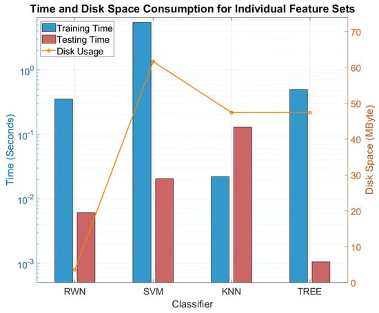
Figure 9.
Time consumption and disk usage for individual feature sets.
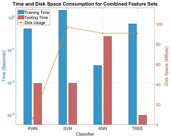
Figure 10.
Time consumption and disk usage for combined feature sets.
Therefore, when considering the combined metrics of high classification accuracy, minimal disk space requirements, and a favorable balance of training/testing times, the RWN emerges as the most well-rounded and efficient classifier for this application. While SVM and KNN offer high accuracy potential, they demand greater computational and storage resources. TREE achieves a balanced trade-off between time and resource usage, but its classification performance does not match the other classifiers.
Having established the performance of the proposed RWN-based feature fusion framework, the final stage of our analysis compares these results against several state-of-the-art machine learning classifiers. Machine learning advancements have led to a variety of classifiers designed to solve complex problems with varying efficiency. To assess our proposed method, we compared its performance with state-of-the-art classifiers. Among these classifiers, CatBoost is a gradient boosting algorithm designed to handle categorical data effectively while mitigating overfitting [48]. Decision trees use a tree-like structure to model decisions and their possible outcomes. They are widely used for both classification and regression problems [49]. The Gaussian Naïve Bayes algorithm, based on Bayes' theorem, is a probabilistic classifier that calculates the likelihood of different classes. It gained popularity for its effectiveness in classification tasks [50]. Gradient boosting methods enhance model performance by iteratively combining weak learners to create a strong predictive model [51]. KNN is a straightforward yet effective algorithm for classification and regression. It assigns class labels by analyzing the nearest k data points in the feature space [52]. LightGBM is a gradient boosting framework optimized for handling large datasets efficiently through distributed learning [53]. Logistic regression is a statistical method used to predict the probability of a dependent variable belonging to a particular category [54]. Random Forests combine multiple decision trees to tackle complex classification problems, improving accuracy and robustness [55]. The Ridge Classifier is an extension of ridge regression; this algorithm is tailored for classification tasks. It excels by incorporating regularization to address overfitting [56]. SVM is an algorithm that finds the most appropriate hyperplane to separate data into different classes and is widely used for both linear and nonlinear problems [57]. XGBoost is a high-performance gradient boosting framework known for its speed and scalability [58]. In Table 21, we present an analysis of the results, highlighting the strengths and generalization capabilities of the proposed approach.
Table 21.
Performance analysis of the proposed method compared to state-of-the-art classifiers.
The comparative results are presented in Table 21. It is crucial to note the experimental setup for this comparison: to provide a robust benchmark, the state-of-the-art classifiers were trained on the best-performing single feature set (ShuffleNet). Our proposed method, by contrast, was trained on the fused ShuffleNet-InceptionV3 feature set to specifically demonstrate the benefit of feature fusion.
The analysis clearly demonstrates the superiority of the proposed method. The RWN-based fusion approach not only achieves the highest average test accuracy of 97.43% but also exhibits the best generalization capability. This is evidenced by the minimal gap between its training and test accuracies, especially when compared to models like LightGBM and XGBoost, which, despite achieving perfect training scores, show a significant performance drop on the test set, indicating severe overfitting.
4. Results and Discussion
This study systematically investigated the performance of a novel feature fusion framework centered on a Random Weight Network (RWN) classifier. The findings directly address the core research questions posed in the Introduction, demonstrating a clear pathway to overcoming the limitations of conventional deep learning models in this challenging security domain.
The investigation first addressed the performance implications of substituting a standard deep learning classifier with an RWN. The results unequivocally demonstrate a significant performance uplift. For instance, on the features extracted from the best-performing standalone model, ShuffleNet, the test accuracy increased dramatically from 83.55% to 94.82% when an RWN with 250 hidden neurons was employed. This finding confirms that by decoupling feature extraction from classification, the inherent performance limitations of conventional models, namely low accuracy and a high propensity for overfitting on complex X-ray data, can be substantially mitigated.
Building upon this, the study validated its primary hypothesis regarding the efficacy of feature fusion. By combining features from different high-performing architectures, notably ShuffleNet and InceptionV3, the framework achieved a state-of-the-art test accuracy of 97.44%. This result provides a definitive affirmative answer to whether multi-model fusion can significantly enhance classification accuracy, clearly outperforming both standalone models and the RWN applied to single feature sets. This highlights that data diversity, achieved through fusing varied feature representations, is a key driver of performance. In contrast, simply duplicating an existing feature set by merging it with itself yields no significant improvement, reinforcing that the richness of the feature pool is what matters.
The performance of the proposed framework was also found to be critically dependent on the careful tuning of RWN’s hyperparameters. Addressing the impact of hidden layer size, the study revealed a clear trade-off: an excessive number of neurons led to overfitting, while an insufficient number resulted in ineffective learning. Optimal generalization was achieved through a balance, with 250 neurons providing the best average test accuracy across many scenarios, and 500 or 1000 neurons yielding the peak accuracy on the best fused dataset. Similarly, the choice of activation function proved significant. Sigmoid, Tangent Sigmoid, and Hardlimit functions consistently delivered superior and robust performance, with Sigmoid ultimately achieving the best overall results. Conversely, other implementation details, such as the order of feature concatenation (N|M vs. M|N), were found to have a negligible impact on the outcome.
In summary, this study confirms that a modular approach, which involves decoupling feature extraction, employing multi-model feature fusion, and utilizing a well-tuned RWN, is a highly effective strategy. This framework successfully answers the initial research challenges, demonstrating a clear pathway from the 83.55% accuracy of standalone models to the 97.44% achieved through the proposed methodology, thereby establishing a new performance benchmark in this security domain.
5. Conclusion and Future Works
This study successfully addressed the challenges of low accuracy and overfitting in deep learning-based X-ray image classification by proposing a novel framework based on feature fusion and a Random Weight Network (RWN) classifier. We demonstrated that by fusing features from diverse, high-performing deep learning architectures, specifically ShuffleNet and InceptionV3, and using a well-tuned RWN, the classification performance can be dramatically improved. The core contribution of this work is the significant increase in test accuracy, from a baseline of 83.55% for the best standalone model to a state-of-the-art 97.44% with the proposed fusion method. Our analysis confirmed that the success of this framework depends not only on the diversity of the fused features but also on the careful tuning of the RWN's hyperparameters, namely the number of hidden neurons and the choice of activation function. This modular approach provides a robust and computationally efficient alternative to end-to-end deep learning systems for this critical security task.
For future work, we plan to expand on these findings by investigating a broader range of feature combination methods and testing the performance of other advanced classifiers. Furthermore, we plan to explore transformer-based feature extraction techniques and deep fusion techniques. In this approach, instead of combining the features after they are fully extracted, the integration would happen at earlier or intermediate stages within a single, unified neural network.
Author Contributions
Conceptualization: M.S.K. and E.E.; Methodology, M.S.K., G.S., E.E. and M.Y.; Software, M.S.K. and G.S.; Validation, M.S.K., G.S., E.E. and X.W.; Formal Analysis, M.S.K. and X.W.; Investigation, G.S. and M.Y.; Resources, M.S.K. and E.E.; Data curation, G.S. and M.Y.; Writing—original draft preparation, M.S.K., G.S. and E.E.; Writing—review and editing, M.S.K., E.E., G.S., M.Y. and X.W.; Visualization, G.S. and M.Y.; Supervision, M.S.K. and X.W.; Project administration, M.S.K. All authors have read and agreed to the published version of the manuscript.
Funding
This research received no external funding.
Institutional Review Board Statement
Not applicable.
Informed Consent Statement
Not applicable.
Data Availability Statement
The data can be available at http://mskiran.ktun.edu.tr/ecd (accessed on 13 August 2025).
Acknowledgments
This study has been supported by the Scientific and Technological Research Council of Türkiye with grant number [122E024]. The authors (M.S. Kiran, E. Esme, G. Seyfi, and M. Yilmaz) would like to thank the council for their institutional support. The author, Xizhao Wang, would like to acknowledge the Stable Support Project of Shenzhen City (No. 20231122124602001).
Conflicts of Interest
The authors declare no conflicts of interest.
References
- Seyfi, G.; Yilmaz, M.; Esme, E.; Kiran, M.S. X-Ray Image Analysis for Explosive Circuit Detection using Deep Learning Algorithms. Appl. Soft Comput. 2023, 151, 11133. [Google Scholar] [CrossRef]
- Wikipedia. X-Ray. Available online: https://en.wikipedia.org/wiki/X-ray (accessed on 26 August 2022).
- Singh, S.; Singh, M. Explosives detection systems (EDS) for aviation security. Signal Process. 2003, 83, 31–55. [Google Scholar] [CrossRef]
- Mery, D.; Riffo, V.; Zuccar, I.; Pieringer, C. Automated X-ray object recognition using an efficient search algorithm in multiple views. In Proceedings of the IEEE Conference on Computer Vision and Pattern Recognition Workshops, Portland, OR, USA, 23–28 June 2013; pp. 368–374. [Google Scholar] [CrossRef]
- Schmidt-Hackenberg, L.; Yousefi, M.R.; Breuel, T.M. Visual cortex inspired features for object detection in X-ray images. In Proceedings of the 21st International Conference on Pattern Recognition (ICPR2012), Tsukuba, Japan, 11–15 November 2012; pp. 2573–2576. [Google Scholar] [CrossRef]
- Akçay, S.; Kundegorski, M.E.; Devereux, M.; Breckon, T.P. Transfer learning using convolutional neural networks for object classification within x-ray baggage security imagery. In Proceedings of the 2016 IEEE International Conference on Image Processing (ICIP), Phonix, AZ, USA, 25–28 September 2016; pp. 1057–1061. [Google Scholar] [CrossRef]
- Jaccard, N.; Rogers, T.W.; Morton, E.J.; Griffin, L.D. Tackling the X-ray cargo inspection challenge using machine learning. In Proceedings of the Anomaly Detection and Imaging with X-Rays (ADIX), Baltimore, MD, USA, 19–20 April 2016; p. 98470N. [Google Scholar] [CrossRef]
- Mery, D.; Svec, E.; Arias, M.; Riffo, V.; Saavedra, J.M.; Banerjee, S. Modern computer vision techniques for x-ray testing in baggage inspection. IEEE Trans. Syst. Man Cybern. Syst. 2016, 47, 682–692. [Google Scholar] [CrossRef]
- Jaccard, N.; Rogers, T.W.; Morton, E.J.; Griffin, L.D. Detection of concealed cars in complex cargo X-ray imagery using deep learning. J. X-Ray Sci. Technol. 2017, 25, 323–339. [Google Scholar] [CrossRef]
- Rogers, T.W.; Jaccard, N.; Griffin, L.D. A deep learning framework for the automated inspection of complex dual-energy X-ray cargo imagery. In Proceedings of the Anomaly Detection and Imaging with X-Rays (ADIX) II, Anaheim, CA, USA, 12–13 April 2017; p. 101870L. [Google Scholar] [CrossRef]
- Caldwell, M.; Ransley, M.; Rogers, T.W.; Griffin, L.D. Transferring x-ray based automated threat detection between scanners with different energies and resolution. In Proceedings of the Counterterrorism, Crime Fighting, Forensics, and Surveillance Technologies, Warsaw, Poland, 11–14 September 2017; p. 104410F. [Google Scholar] [CrossRef]
- Morris, T.; Chien, T.; Goodman, E. Convolutional neural networks for automatic threat detection in security X-Ray images. In Proceedings of the 17th IEEE International Conference on Machine Learning and Applications (ICMLA), Orlando, FL, USA, 17–20 December 2018; pp. 285–292. [Google Scholar] [CrossRef]
- Akcay, S.; Breckon, T.P. An evaluation of region based object detection strategies within X-ray baggage security imagery. In Proceedings of the IEEE International Conference on Image Processing (ICIP), Beijing, China, 17–20 September 2017; pp. 1337–1341. [Google Scholar] [CrossRef]
- Akcay, S.; Kundegorski, M.E.; Willcocks, C.G.; Breckon, T.P. Using deep convolutional neural network architectures for object classification and detection within x-ray baggage security imagery. IEEE Trans. Inf. Forensics Secur. 2018, 13, 2203–2215. [Google Scholar] [CrossRef]
- Petrozziello, A.; Jordanov, I. Automated deep learning for threat detection in luggage from X-ray images. In Proceedings of the International Symposium on Experimental Algorithms, Kalamata, Greece, 24–29 June 2019; pp. 505–512. [Google Scholar] [CrossRef]
- Cheng, Q.; Lan, T.; Cai, Z.; Li, J. X-YOLO: An Efficient Detection Network of Dangerous Objects in X-ray Baggage Images. IEEE Signal Process. Lett. 2024, 31, 2270–2274. [Google Scholar] [CrossRef]
- Wu, J.; Xu, X. EslaXDET: A new X-ray baggage security detection framework based on self-supervised vision transformers. Eng. Appl. Artif. Intell. 2024, 127, 107440. [Google Scholar] [CrossRef]
- Wang, S.; Wang, S.; Xiao, Z. Feature extraction method with efficient edge information enhancement for detecting dangerous objects in security x-ray images. In Proceedings of the International Conference on Computer Graphics, Artificial Intelligence, and Data Processing (ICCAID 2024), Nanchang, China, 13–15 December 2025; pp. 95–106. [Google Scholar] [CrossRef]
- Yang, J.; Zhao, Z.; Zhang, H.; Shi, Y. Data augmentation for X-ray prohibited item images using generative adversarial networks. IEEE Access 2019, 7, 28894–28902. [Google Scholar] [CrossRef]
- Kaminetzky, A.; Mery, D. In-depth analysis of automated baggage inspection using simulated X-ray images of 3D models. Neural Comput. Appl. 2024, 36, 18761–18780. [Google Scholar] [CrossRef]
- Caldwell, M.; Griffin, L.D. Limits on transfer learning from photographic image data to X-ray threat detection. J. X-Ray Sci. Technol. 2019, 27, 1007–1020. [Google Scholar] [CrossRef]
- Benedykciuk, E.; Denkowski, M.; Dmitruk, K. Material classification in X-ray images based on multi-scale CNN. Signal Image Video Process. 2021, 15, 1285–1293. [Google Scholar] [CrossRef]
- Babalik, A.; Babadag, A. A binary sparrow search algorithm for feature selection on classification of X-ray security images. Appl. Soft Comput. 2024, 158, 111546. [Google Scholar] [CrossRef]
- Ayantayo, A.; Kaur, A.; Kour, A.; Schmoor, X.; Shah, F.; Vickers, I.; Kearney, P.; Abdelsamea, M.M. Network intrusion detection using feature fusion with deep learning. J. Big Data 2023, 10, 167. [Google Scholar] [CrossRef]
- Zhang, K.; Ting, H.-N.; Choo, Y.-M. Baby cry recognition by BCRNet using transfer learning and deep feature fusion. IEEE Access 2023, 11, 126251–126262. [Google Scholar] [CrossRef]
- Wu, X.; Shi, H.; Zhu, H. Fault Diagnosis for Rolling Bearings Based on Multiscale Feature Fusion Deep Residual Networks. Electronics 2023, 12, 768. [Google Scholar] [CrossRef]
- Liu, H.; Hou, C.-J.; Tang, J.-L.; Sun, L.-T.; Lu, K.-F.; Liu, Y.; Du, P. Deep learning and ultrasound feature fusion model predicts the malignancy of complex cystic and solid breast nodules with color Doppler images. Sci. Rep. 2023, 13, 10500. [Google Scholar] [CrossRef]
- Patil, S.; Kirange, D. An Optimized Deep Learning Model with Feature Fusion for Brain Tumor Detection. Int. J. Next-Gener. Comput. 2023, 14. [Google Scholar] [CrossRef]
- Gill, H.S.; Murugesan, G.; Mehbodniya, A.; Sajja, G.S.; Gupta, G.; Bhatt, A. Fruit type classification using deep learning and feature fusion. Comput. Electron. Agric. 2023, 211, 107990. [Google Scholar] [CrossRef]
- Deng, T.; Wang, H.; He, D.; Xiong, N.; Liang, W.; Wang, J. Multi-Dimensional Fusion Deep Learning for Side Channel Analysis. Electronics 2023, 12, 4728. [Google Scholar] [CrossRef]
- Al-Timemy, A.H.; Alzubaidi, L.; Mosa, Z.M.; Abdelmotaal, H.; Ghaeb, N.H.; Lavric, A.; Hazarbassanov, R.M.; Takahashi, H.; Gu, Y.; Yousefi, S. A Deep Feature Fusion of Improved Suspected Keratoconus Detection with Deep Learning. Diagnostics 2023, 13, 1689. [Google Scholar] [CrossRef]
- Peng, Y.; Zhang, J. Lung lobe segmentation in computed tomography images based on multi-feature fusion and ensemble learning framework. Int. J. Imaging Syst. Technol. 2023, 33, 2088–2099. [Google Scholar] [CrossRef]
- Tu, C.; Bai, R.; Aickelin, U.; Zhang, Y.; Du, H. A deep reinforcement learning hyper-heuristic with feature fusion for online packing problems. Expert Syst. Appl. 2023, 230, 120568. [Google Scholar] [CrossRef]
- Tan, J.; Wan, J.; Xia, D. Automobile Component Recognition Based on Deep Learning Network with Coarse-Fine-Grained Feature Fusion. Int. J. Intell. Syst. 2023, 2023, 1903292. [Google Scholar] [CrossRef]
- Medjahed, C.; Mezzoudj, F.; Rahmoun, A.; Charrier, C. Identification based on feature fusion of multimodal biometrics and deep learning. Int. J. Biom. 2023, 15, 521–538. [Google Scholar] [CrossRef]
- Ma, J.; Zhang, Y.; Li, Y.; Zhou, L.; Qin, L.; Zeng, Y.; Wang, P.; Lei, Y. Deep dual-side learning ensemble model for Parkinson speech recognition. Biomed. Signal Process. Control 2021, 69, 102849. [Google Scholar] [CrossRef]
- Alzubaidi, L.; Salhi, A.; A. Fadhel, M.; Bai, J.; Hollman, F.; Italia, K.; Pareyon, R.; Albahri, A.; Ouyang, C.; Santamaría, J. Trustworthy deep learning framework for the detection of abnormalities in X-ray shoulder images. PLoS ONE 2024, 19, e0299545. [Google Scholar] [CrossRef]
- Agarwal, S.; Arya, K.; Meena, Y.K. Multifusionnet: Multilayer multimodal fusion of deep neural networks for chest x-ray image classification. arXiv 2024, arXiv:2401.00728. [Google Scholar] [CrossRef]
- Li, J.; Shan, H.-J.; Yu, X.-W. Fracture detection of distal radius using deep-learning-based dual-channel feature fusion algorithm. Chin. J. Traumatol. 2025, 1–13. [Google Scholar] [CrossRef]
- Seyfi, G.; Esme, E.; Yilmaz, M.; Kiran, M.S. A literature review on deep learning algorithms for analysis of X-ray images. Int. J. Mach. Learn. Cybern. 2024, 15, 1165–1181. [Google Scholar] [CrossRef]
- Sani, S.; Wiratunga, N.; Massie, S. Learning deep features for kNN-based human activity recognition. In Proceedings of the ICCBR 2017 Workshops, Trondheim, Norway, 26–28 June 2017. [Google Scholar] [CrossRef]
- Singh, J.; Thakur, D.; Ali, F.; Gera, T.; Kwak, K.S. Deep feature extraction and classification of android malware images. Sensors 2020, 20, 7013. [Google Scholar] [CrossRef]
- Benyahia, S.; Meftah, B.; Lézoray, O. Multi-features extraction based on deep learning for skin lesion classification. Tissue Cell 2022, 74, 101701. [Google Scholar] [CrossRef]
- Pao, Y.-H.; Takefuji, Y. Functional-link net computing: Theory, system architecture, and functionalities. Computer 1992, 25, 76–79. [Google Scholar] [CrossRef]
- Schmidt, W.F.; Kraaijveld, M.A.; Duin, R.P. Feed forward neural networks with random weights. In Proceedings of the International Conference on Pattern Recognition, The Hague, The Netherlands, 30 August–3 September 1992; p. 1. [Google Scholar] [CrossRef]
- Huang, G.-B.; Zhu, Q.-Y.; Siew, C.-K. Extreme learning machine: A new learning scheme of feedforward neural networks. In Proceedings of the IEEE international Joint Conference on Neural Networks (IEEE Cat. No. 04CH37541), Budapest, Hungary, 25–29 July 2004; pp. 985–990. [Google Scholar] [CrossRef]
- Huang, G.-B.; Zhu, Q.-Y.; Siew, C.-K. Extreme learning machine: Theory and applications. Neurocomputing 2006, 70, 489–501. [Google Scholar] [CrossRef]
- Dorogush, A.V.; Ershov, V.; Gulin, A. CatBoost: Gradient boosting with categorical features support. arXiv 2018, arXiv:1810.11363. [Google Scholar] [CrossRef]
- Quinlan, J.R. C4.5: Programs for Machine Learning; Elsevier: Amsterdam, The Netherlands, 2014. [Google Scholar] [CrossRef]
- Mitchell, T.M.; Mitchell, T.M. Machine Learning; McGraw-Hill: New York, NY, USA, 1997; Volume 1. [Google Scholar]
- Natekin, A.; Knoll, A. Gradient boosting machines, a tutorial. Front. Neurorobot. 2013, 7, 21. [Google Scholar] [CrossRef]
- Cover, T.; Hart, P. Nearest neighbor pattern classification. IEEE Trans. Inf. Theory 1967, 13, 21–27. [Google Scholar] [CrossRef]
- Ke, G.; Meng, Q.; Finley, T.; Wang, T.; Chen, W.; Ma, W.; Ye, Q.; Liu, T.-Y. Lightgbm: A highly efficient gradient boosting decision tree. Adv. Neural Inf. Process. Syst. 2017, 30. [Google Scholar]
- Cox, D.R. The regression analysis of binary sequences. J. R. Stat. Soc. Ser. B Stat. Methodol. 1958, 20, 215–232. [Google Scholar] [CrossRef]
- Breiman, L. Random forests. Mach. Learn. 2001, 45, 5–32. [Google Scholar] [CrossRef]
- Hoerl, A.E.; Kennard, R.W. Ridge regression: Biased estimation for nonorthogonal problems. Technometrics 1970, 12, 55–67. [Google Scholar] [CrossRef]
- Cortes, C.; Vapnik, V. Support-Vector Networks. In Machine Learning; Springer: Berlin/Heidelberg, Germany, 1995. [Google Scholar]
- Chen, T.; Guestrin, C. Xgboost: A scalable tree boosting system. In Proceedings of the 22nd ACM SIGKDD International Conference on Knowledge Discovery and Data Mining, San Francisco, CA, USA, 13–17 August 2016; pp. 785–794. [Google Scholar] [CrossRef]
Disclaimer/Publisher’s Note: The statements, opinions and data contained in all publications are solely those of the individual author(s) and contributor(s) and not of MDPI and/or the editor(s). MDPI and/or the editor(s) disclaim responsibility for any injury to people or property resulting from any ideas, methods, instructions or products referred to in the content. |
© 2025 by the authors. Licensee MDPI, Basel, Switzerland. This article is an open access article distributed under the terms and conditions of the Creative Commons Attribution (CC BY) license (https://creativecommons.org/licenses/by/4.0/).