A Physical-Enhanced Spatio-Temporal Graph Convolutional Network for River Flow Prediction

Abstract

River flow forecasting remains a critical yet challenging task in hydrological science, owing to the inherent trade-offs between physics-based models and data-driven methods. While physics-based models offer interpretability and process-based insights, they often struggle with real-world complexity and adaptability. Conversely, purely data-driven models, though powerful in capturing data patterns, lack physical grounding and often underperform in extreme scenarios. To address this gap, we propose PESTGCN, a Physical-Enhanced Spatio-Temporal Graph Convolutional Network that integrates hydrological domain knowledge with the flexibility of graph-based learning. PESTGCN models the watershed system as a Heterogeneous Information Network (HIN), capturing various physical entities (e.g., gauge stations, rainfall stations, reservoirs) and their diverse interactions (e.g., spatial proximity, rainfall influence, and regulation effects) within a unified graph structure. To better capture the latent semantics, meta-path-based encoding is employed to model higher-order relationships. Furthermore, a hybrid attention mechanism incorporating both local temporal features and global spatial dependencies enables comprehensive sequence learning. Importantly, key variables from the HEC-HMS hydrological model are embedded into the framework to improve physical interpretability and generalization. Experimental results on four real-world benchmark watersheds demonstrate that PESTGCN achieves statistically significant improvements over existing state-of-the-art models, with relative reductions in MAE ranging from 5.3% to 13.6% across different forecast horizons. These results validate the effectiveness of combining physical priors with graph-based temporal modeling.

1. Introduction

The intensified impacts of natural changes and human activities have caused runoff signals to exhibit multi-scale temporal variability and non-stationary characteristics, posing significant challenges to runoff forecasting and flood prediction [1,2]. Although extensive research has been conducted in this area, hydrologists still urgently require more accurate and efficient forecasting models tailored to different basins and environmental conditions. Traditional flood forecasting models are broadly categorized into lumped models and distributed models. Lumped models treat the entire watershed as a single entity by averaging variables and parameters, thus simplifying the simulation of precipitation–runoff relationships [3]. Due to the complexity of hydrological processes, lumped models typically require manual calibration or algorithmic optimization to achieve reliable performance. In contrast, distributed models, grounded in the physical principles of the hydrological cycle, represent spatial heterogeneity explicitly [4]. Their parameters possess physical significance and can often be calibrated based on field measurements, offering enhanced scientific value and reduced model development complexity [5].

Nevertheless, both lumped and distributed models still face notable limitations, particularly in capturing nonlinear dependencies, handling large-scale data, and adapting to diverse environmental scenarios. As a result, researchers have increasingly turned to data-driven approaches, which offer greater flexibility and learning capacity from observed data.

In recent years, data-driven approaches, particularly those based on deep learning, have emerged as powerful alternatives for flood prediction. Deep learning, with neural networks at its core, excels at modeling complex nonlinear relationships [6]. Among these approaches, hybrid models have shown promising results. For instance, the WNN-SVM model developed by Yu Yang’s team combined wavelet neural networks and support vector machines, significantly improving predictive accuracy in hydrological time series forecasting through extensive field experiments in the Tunxi River Basin [7]. The backpropagation (BP) neural network, a classic feedforward structure trained via error backpropagation, has also been widely applied in flood forecasting [8]. Studies such as those conducted by Hou Xiang’s team in the Jialing River Basin [9] and Yuan Jing’s team at the Yichang hydrological station [10] demonstrated that BP networks could effectively capture the complex and uncertain relationships between rainfall and runoff, achieving satisfactory predictive performance in short-term forecasting scenarios.

Advancements in recurrent neural networks (RNNs) have introduced more sophisticated architectures like the Long Short-Term Memory (LSTM) and Gated Recurrent Unit (GRU) networks, which exhibit superior capabilities in modeling temporal dependencies [11]. Considering the sequential nature of rainfall–runoff processes, these models have been increasingly employed in hydrology. Xu Yuanhao et al. [12] utilized LSTM networks for flood prediction in the middle reaches of the Yellow River, achieving high accuracy for short-term forecasts, though with decreased performance over longer prediction horizons. Duan Shengyue et al. [13] introduced a regularized GRU-based model that demonstrated improved generalization in the Ganjiang River Basin. Liang Xiaoxu et al. [14] further enhanced GRU models by incorporating attention mechanisms, achieving high-precision forecasting in the Wuyuan region. However, the experimental results showed that the model could achieve high-precision prediction of river flow within a 26 h anticipation period. Nevertheless, since this model merely conducted in-depth mining of time series information and did not take into account the spatial distribution information of rainfall, its prediction performance was poor in cases of heavy rainfall in localized areas. Moreover, the structure of the model was relatively complex, and its response was slow.

To more effectively leverage spatial dependencies in hydrological systems, convolutional neural networks (CNNs) have been increasingly applied to flood forecasting tasks. Initially proposed by LeCun et al. [15], CNNs are well-suited for processing structured spatial data due to their inherent two-dimensional feature extraction capabilities, enabling integration of topographical and hydrometeorological inputs. For instance, Hui Qiang et al. [16] developed a CNN-based framework that transformed rainfall station observations into gridded data to capture spatial rainfall distribution, achieving promising performance in forecasting river discharge in the Xixian region of Henan Province. However, the gridding process significantly increased data dimensionality, imposing high computational demands and leading to overfitting risks when training samples were limited.

Complementarily, Wang Yi et al. [17] proposed a hybrid model combining CNNs and support vector machines (SVMs) to assess flood susceptibility based on remote sensing imagery, terrain morphology, and digital elevation data. While the model demonstrated strong classification accuracy in identifying flood-prone areas, it did not produce quantitative forecasts of river discharge or water levels, thereby limiting its operational utility in real-time flood early warning and decision-making systems.

Recent developments in graph neural networks (GNNs) have further advanced spatial information integration by modeling non-Euclidean relationships. Luan Dingbin et al. [18] proposed the GC-RNN model, abstracting rainfall stations as nodes and river connectivity as edges, thereby embedding spatial rainfall distribution into the network structure. Although the model performed satisfactorily under moderate rainfall conditions, prediction accuracy deteriorated during heavy rainfall events due to insufficient sample sizes. Furthermore, Zhao Song et al. [19] proposed the CAe-RNN model, combining graph convolutional operations with recurrent structures to effectively extract and fuse spatial–temporal features. Field evaluations demonstrated that the model maintained high accuracy across different forecast lead times and met hydrological standards for flood peak magnitude and timing prediction.

Data-driven models have gained increasing popularity in river flow forecasting due to their ability to learn complex temporal patterns directly from observed data without requiring explicit knowledge of underlying hydrological processes. Their advantages include ease of deployment, flexibility in modeling nonlinear dynamics, and adaptability to diverse data conditions. These models can be rapidly trained and updated as new data become available, making them well-suited for real-time applications and operational forecasting.

Despite these advances, river flow prediction as a typical spatiotemporal forecasting problem still faces several critical challenges. First, although these models are proficient at capturing statistical dependencies from historical observations, they typically lack physical interpretability and perform poorly under extrapolative scenarios. In contrast, runoff generation is fundamentally driven by hydrological processes such as precipitation, infiltration, evaporation, and soil–moisture interactions, all of which are spatiotemporally heterogeneous. Purely data-driven methods struggle to represent these complex dynamics, especially under extreme events like heavy rainfall or drought, where the lack of precedent in the training data may cause prediction failures. In such cases, physics-based models, by quantifying variables such as soil water retention capacity or surface runoff thresholds, can capture the dynamic response of watersheds more accurately. Therefore, integrating physical hydrological mechanisms into data-driven frameworks not only enhances forecast accuracy but also improves robustness and generalization, particularly under climate variability and anthropogenic influences.

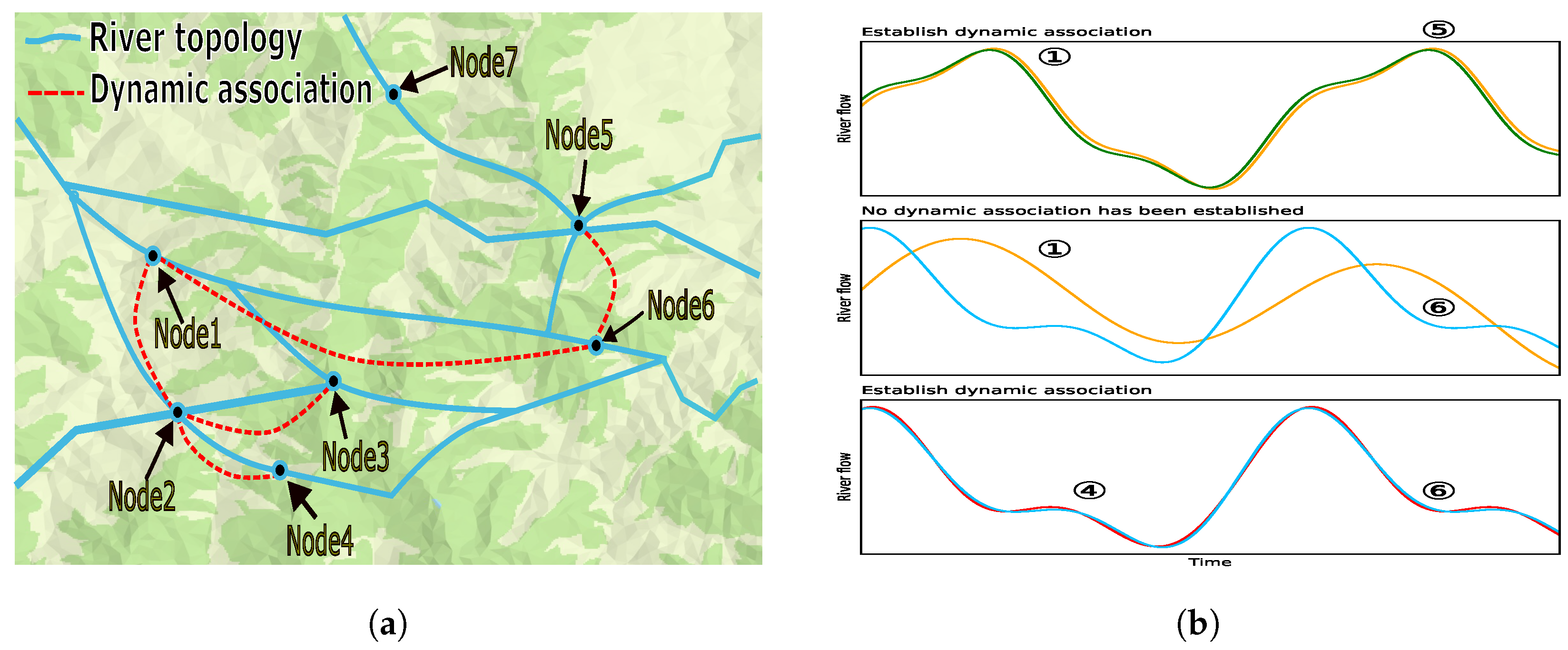
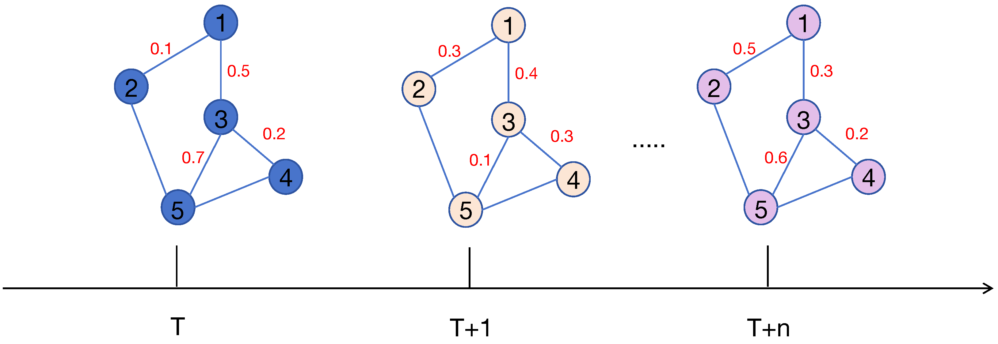
A second significant challenge is capturing the temporal similarity and dynamic spatiotemporal correlations among river network nodes. Most graph convolution-based models depend on pre-defined static graphs to represent spatial relationships [20], a method that falls short because river flows vary dynamically over time and space. Static graphs often fail to represent non-obvious, yet crucial, relationships. As shown in Figure 1, for example, nodes 1 and 5 are not directly connected and are far apart, but their similar riverine conditions resulted in comparable flow patterns. A similar dynamic relationship existed between nodes 4 and 6. Conversely, nodes 1 and 6, which were distant and in different environments, were harder to associate dynamically. This suggests that analyzing similarities in discharge time series can uncover regional hydrological likenesses, an insight that is critical for improving the accuracy and generalization of predictions. To overcome the limitations of static graphs, some approaches, like STFGNN [21], have used dynamic time warping (DTW) to assess temporal similarity. Nevertheless, these methods still did not fully capture the complex dynamic spatiotemporal dependencies between river nodes.

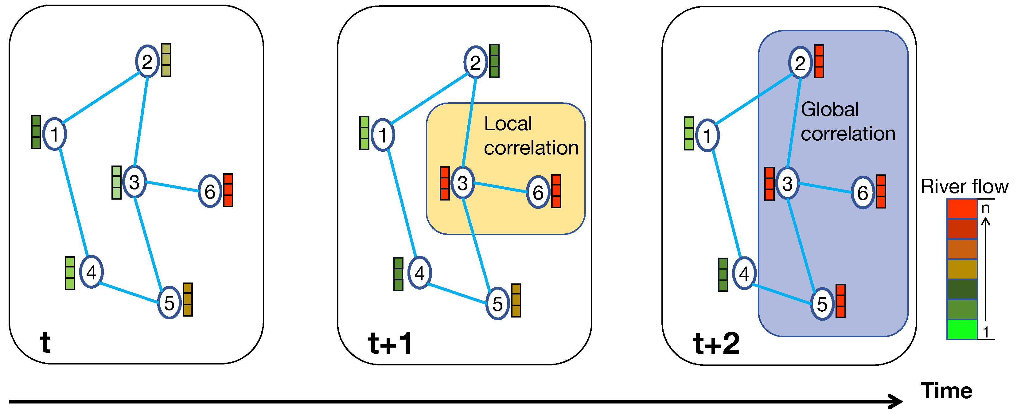
Thirdly, it remains challenging to simultaneously model both local and global spatial dependencies within river networks. In such complex systems, the state of a single node can significantly influence distant nodes through hydraulic interactions [22]. As a highly connected and spatiotemporally correlated structure, the river network exhibits complex interdependencies that are not confined to local regions; correlations can exist even between spatially distant nodes. These dependencies, such as interactions and associations, can influence the overall flow dynamics of the entire network. For instance, as shown in Figure 2, an excessive flow at node 6 may lead to turbulent conditions at the nearby node 3 (a local effect) while also affecting the hydrodynamics at distant nodes 2 and 5 (a global effect), thereby altering the flow state across the network. Therefore, effectively capturing both local spatial structures and global spatial dependencies is crucial for enhancing the accuracy of river flow predictions. However, most current models neglect these global interactions by focusing primarily on local structures, which limits their prediction accuracy for network-wide hydrodynamic behaviors [23].

Recent developments in graph-based deep learning have demonstrated the effectiveness of combining graph structures with attention mechanisms for spatiotemporal forecasting tasks. For example, SmartFormer [24] employs a graph-based transformer architecture to model energy load dynamics, showcasing the potential of hybrid models in capturing complex spatial and temporal dependencies. Motivated by these advances, our study focuses on river flow prediction—an equally challenging environmental time-series task—by proposing a new hybrid framework that integrates heterogeneous graph modeling with physical domain knowledge.

To address these challenges, we propose a novel Physical-Enhanced Spatio-Temporal Graph Convolutional Network (PESTGCN) for river flow forecasting. In PESTGCN, a physical model of runoff generation is incorporated into the data-driven river flow prediction framework. Instead of constructing separate graphs, the method characterizes the complex watershed system as a single, unified heterogeneous graph. This advanced framework integrates diverse relationships—such as static river network topology, dynamic temporal similarity metrics, and causal links between different physical entities—into a comprehensive structure. The unified graph is processed by heterogeneous graph convolution modules enhanced with self-attention mechanisms to capture rich, multi-faceted dependencies. Furthermore, PESTGCN introduces global feature learning to capture long-term spatiotemporal dependencies and interactions between local and global structures within the river network. Finally, a context-aware temporal module employing multi-head self-attention is used to extract complex temporal dependencies, enabling accurate predictions of future river flow states.

The major contributions of this work are summarized as follows:

(1) Integration of physical mechanisms for enhanced robustness: To address the limitations of purely data-driven models in representing hydrological processes—particularly under extreme climatic events [25]—we incorporate a physical model of runoff generation into the learning framework. By embedding hydrological simulation outputs such as canopy interception, surface evaporation, and deep infiltration derived from the HEC-HMS model, PESTGCN captures key physical mechanisms (e.g., soil moisture dynamics and runoff thresholds) [26]. This integration improves interpretability, enhances generalization to unseen conditions, and significantly increases robustness against data sparsity and climatic extremes.

(2) Development of a unified heterogeneous graph architecture: To effectively model the complex and multi-faceted dependencies in river systems, we design a unified heterogeneous graph that represents the watershed as a rich information network. This graph incorporates multiple types of nodes (e.g., gauge stations, rainfall stations, reservoirs) and diverse relations (e.g., physical adjacency, temporal similarity, engineering regulation). By learning simultaneously from static topology, dynamic correlations, and causal physical interactions, PESTGCN achieves a more comprehensive representation of watershed dynamics, which is crucial for accurate river flow forecasting.

2. Methods

2.1. Problem Definition for River Flow Forecasting

To formalize the river flow forecasting task, this work first defines the spatiotemporal structure of the river network. Let the river flow dynamic network be represented by three distinct but related graphs: a spatial structure graph $G^S=(V,E^S,{\mathbf{A}}^S)$, a dynamic association graph $G^D=(V,E^D,{\mathbf{A}}^D)$, and a semantic meta-path graph $G^P=(V,E^P,{\mathbf{A}}^P)$. Here, V denotes the set of nodes, with $\left|V\right|=N$ representing the number of observation nodes, such as river flow gauges or velocity sensors. All three graphs share the same node set but differ in their edge definitions and edge weights. Specifically, $E^S$, $E^D$, and $E^P$ denote the edge sets of the spatial, dynamic, and semantic graphs, respectively, while ${\mathbf{A}}^S$, ${\mathbf{A}}^D$, and ${\mathbf{A}}^P$ are the corresponding adjacency matrices describing the connectivity relationships between nodes in each graph.

The spatial structure graph $G^S$ captures the static topology of the river network, where edges represent physical adjacency (e.g., direct upstream–downstream connections). The dynamic association graph $G^D$ models temporal similarity between nodes based on their historical discharge patterns, enabling the representation of dynamic and non-obvious correlations. The semantic meta-path graph $G^P$ encodes higher-order semantic associations derived from multi-step composite relationships among nodes—those not easily represented by a single direct edge. For example, a meta-path such as “upstream-to-downstream through confluence” has explicit hydrological meaning. The adjacency matrix ${\mathbf{A}}^P$ is obtained by multiplying the adjacency matrices of all constituent relations along this meta-path, producing a composite matrix that encodes the strength of these complex semantic connections.

Let ${\mathbf{X}}_t=\{{\mathbf{x}}_{t,1},{\mathbf{x}}_{t,2},\dots ,{\mathbf{x}}_{t,N}\}\in {\mathbb{R}}^{N\times C}$ denote the matrix of observed node features at time t, where ${\mathbf{x}}_{t,n}\in {\mathbb{R}}^C$ is the feature vector of node n that includes observed flow, velocity, and other relevant attributes. The river flow vector at time t is defined as ${\mathbf{y}}_t=[y_{t,1},y_{t,2},\dots ,y_{t,N}]$, where $y_{t,n}$ represents the flow at node n.

The objective of river flow forecasting is to learn a function f that maps a sequence of historical node features and network structures to future river flow predictions. Given a historical observation window of length T, the model aims to predict the river flows at all N nodes over the next M time steps. This can be expressed as:

$$[{\mathbf{y}}_{t+1},{\mathbf{y}}_{t+2},\dots ,{\mathbf{y}}_{t+M}]=f({\mathbf{X}}_{t-T+1},\dots ,{\mathbf{X}}_t;G),$$

where G collectively denotes the graph structure information (including $G^S$, $G^D$, and $G^P$), and f captures the spatiotemporal dependencies across the river network to enable accurate multi-step forecasting.

2.2. Runoff Generation Model

2.2.1. HEC-HMS Hydrological Model

The Hydrologic Engineering Center–Hydrologic Modeling System (HEC-HMS) is a distributed hydrological model developed by the U.S. Army Corps of Engineers [27]. It is widely used for simulating watershed-scale hydrological processes and supports applications such as flood forecasting, water resources planning, and hydrologic impact assessment. As illustrated in Figure 3, HEC-HMS can simulate key processes including precipitation, evaporation, infiltration, soil moisture dynamics, and runoff generation across different spatial and temporal scales, thereby providing reliable predictions of watershed runoff.

In the runoff generation module, HEC-HMS represents the hydrological process through three components: canopy interception, surface evaporation, and subsurface percolation. The canopy interception process is modeled using a conceptual storage approach, where precipitation is initially retained by the canopy until the interception capacity is reached; subsequent excess water either evaporates or infiltrates into the ground. Surface evaporation accounts for the direct loss of water from the land surface to the atmosphere, governed by thermodynamic and aerodynamic interactions influenced by temperature, humidity, and wind speed. Subsurface percolation describes the downward movement of infiltrated water into deeper soil layers, with the influence of fine-scale topographic variation neglected in the current formulation.

Based on the above processes, the runoff mass balance at time t can be expressed as:

$$P\left(t\right)=E_{\mathrm{c}}\left(t\right)+E_{\mathrm{s}}\left(t\right)+I_{\mathrm{g}}\left(t\right),$$

(1)

where $P\left(t\right)$ denotes the runoff generation rate at time t, $E_{\mathrm{c}}\left(t\right)$ is the canopy interception loss, $E_{\mathrm{s}}\left(t\right)$ represents surface evaporation, and $I_{\mathrm{g}}\left(t\right)$ corresponds to subsurface percolation. The canopy interception process $E_{\mathrm{c}}\left(t\right)$ is governed by the following water balance equation:

$${\displaystyle \frac{d{E}_{\mathrm{c}}\left(t\right)}{dt}}=I_{\mathrm{rain}}-E-D_{\mathrm{drain}},$$

(2)

where S is the instantaneous water storage in the canopy (mm), $I_{\mathrm{rain}}$ is the precipitation input rate (mm/h), E is the evaporation rate (mm/h), and $D_{\mathrm{drain}}$ is the drainage rate (mm/h). Surface evaporation $E_{\mathrm{s}}\left(t\right)$ is determined empirically using the Hargreaves equation:

$${\displaystyle \frac{d{E}_{\mathrm{s}}\left(t\right)}{dt}}=0.0023·R_a·(T_{\mathrm{avg}}+17.8)·{(T_{\max }-T_{\min })}^{0.5},$$

(3)

where $R_a$ denotes extraterrestrial solar radiation (MJ/m²/day), $T_{\mathrm{avg}}$ is the average daily temperature (°C), $T_{\max }$ and $T_{\min }$ are the daily maximum and minimum temperatures (°C), respectively. The subsurface percolation $I_{\mathrm{g}}\left(t\right)$ is modeled using numerical solutions to the Richards equation:

$${\displaystyle \frac{d{I}_g\left(t\right)}{dt}}=\left[K_s·S_e^l\left(t\right)·(h+1)\right]·D,$$

(4)

where $k_s$ denotes the saturated hydraulic conductivity, $S_e^l\left(t\right)$ is the current effective saturation, h represents the soil water potential, and D is the average depth of the study region.

In the HEC-HMS framework, hydrological variables such as the canopy interception loss rate $E_c\left(t\right)$, the surface evaporation rate $E_s\left(t\right)$, and the subsurface percolation rate $I_g\left(t\right)$ are expressed as time-varying instantaneous rates. To obtain their total amounts over a specified time interval $[t_1,t_2]$, these rate functions must be integrated. Due to the complexity of their temporal variations, analytical integration is generally intractable. Therefore, this study applies numerical integration to approximate the cumulative quantities. The interval $[t_1,t_2]$ is discretized into a sequence of small, consecutive time steps $\mathrm{\Delta }t$. For each time step, the incremental quantity is calculated as the product of the average rate during that step and the step length $\mathrm{\Delta }t$. The total canopy interception loss, surface evaporation, and subsurface percolation are then obtained by summing the incremental quantities over all time steps within the interval.

2.2.2. Incorporate Physical Modeling Information

To incorporate physical modeling information, this work combines the HEC-HMS hydrological model to simulate the flow generation process and obtains the flow generation $P_{t,n}^{\mathrm{HMS}}\in \mathbb{R}$ of each node at time t, which is calculated as:

$$P_{t,n}^{\mathrm{HMS}}={\int }_t^{t+\mathrm{\Delta }t}P\left(t\right)dt,$$

(5)

where $P\left(t\right)$ is defined in Equation (1), $\mathrm{\Delta }t$ is the time step of time series.

After concatenating this physical feature with the original observation vector, an enhanced feature can be reformed as $\mathbf{x}{’}_{t,n}=[{\mathbf{x}}_{t,n};P_{t,n}^{\mathrm{HMS}}]\in {\mathbb{R}}^{C+1}$. Accordingly, the enhanced feature matrix is reformued as: ${\mathbf{X}}_t^{\prime }=({\mathbf{x}}_{t,1}^{\prime },{\mathbf{x}}_{t,2}^{\prime },\dots ,{\mathbf{x}}_{t,N}^{\prime })\in {\mathbb{R}}^{N\times (C+1)}$.

The river flow vector at time t is defined as ${\mathbf{y}}_t=[y_{t,1},y_{t,2},\dots ,y_{t,N}]$, where $y_{t,n}$ represents the flow at node n. The objective of river flow forecasting is to learn a function f that maps a sequence of historical node features and network structure into future river flow predictions. Given a historical observation window of length T, the model aims to predict the river flows at all N nodes over the next M time steps can be reformulated as: $[y_{t+1},y_{t+2},\dots ,y_{t+M}]=f({\mathbf{X}}_{t-T+1}^{\prime },\dots ,{\mathbf{X}}_t^{\prime };G)$.

2.3. The Construction of Multi-View Graph Structure

2.3.1. Spatial Structure Graph $G^S$

The core task of river flow forecasting is to predict future variations in discharge based on historical observations and the complex interdependencies among monitoring nodes within a watershed. In this study, the N observation nodes (e.g., flow gauges or velocity sensors) are defined as a set V, with the observed features at time step t represented by a feature matrix ${\mathbf{X}}_t\in {\mathbb{R}}^{N\times C}$, where C denotes the number of features per node, such as flow rate and velocity.

Modeling each node independently as a univariate time series overlooks the spatial dependencies inherent in river systems. These dependencies—arising from physical processes such as upstream flow propagation and hydrological confluence—create strong correlations among nodes. Therefore, to achieve accurate river flow forecasting, it is essential to incorporate not only temporal patterns but also spatial interactions between nodes into the forecasting framework.

Given the heterogeneous nature of these spatial interactions, which include both static topological connections and dynamic functional similarities, a single graph representation is insufficient to capture all relevant dependencies. To address this, we adopt a multi-view graph modeling approach, in which two complementary graph structures are constructed: a spatial structure graph $G^S$, designed to encode the fixed physical layout and connectivity of the watershed, and a dynamic association graph $G^D$, introduced to capture time-dependent functional relationships among nodes. This dual-graph formulation enables a more comprehensive and structured representation of spatial heterogeneity in the river network.

The spatial structure graph, denoted as $G^S=(V,E^S,{\mathbf{A}}^S)$, represents the static physical topology of the river network. Here, the node set V corresponds to the same N observation nodes, while the edge set $E^S$ captures the actual river channel connections between these nodes. The corresponding adjacency matrix ${\mathbf{A}}^S\in {\mathbb{R}}^{N\times N}$ is weighted, with each entry ${\mathbf{A}}_{ij}^S$ quantifying the spatial proximity or connectivity strength between node i and node j. This connectivity is modeled using a Gaussian kernel based on river channel distance $d_{ij}$, defined as:

$${\mathbf{A}}_{ij}^S=exp\left(-{\displaystyle \frac{d_{ij}^2}{{\sigma }^2}}\right),$$

(6)

where ${\sigma }^2$ controls the spatial decay. Since the river topology remains fixed over the forecasting horizon, $G^S$ serves as a static prior that provides essential structural information for modeling flow propagation in real-world scenarios.

2.3.2. Dynamic Association Graph $G^D$

The dynamic association graph, $G^D=(V,E^D,{\mathbf{A}}^D)$, is designed to capture data-driven functional dependencies that cannot be inferred solely from the physical topology. In hydrological systems, two geographically distant nodes with no direct waterway connection may still exhibit highly synchronous flow patterns due to similar catchment characteristics or exposure to the same weather systems. To represent such “teleconnections” or functional similarities, it is necessary to assess the similarity between the historical time series of different nodes. However, simple distance metrics such as the Euclidean distance are highly sensitive to minor shifts, stretching, or compression along the time axis—a common phenomenon in hydrology, for example, when a flood peak arrives several hours earlier at an upstream station than at a downstream one. In such cases, Euclidean distance would incorrectly penalize phase-shifted yet morphologically similar sequences as being dissimilar.

To address this issue, we employ the dynamic time warping (DTW) algorithm to measure the similarity between the historical flow time series of any two nodes, i and j. DTW is a robust technique that determines an optimal alignment between two time series by non-linearly “warping” the time axis of one sequence to match the other, thereby providing a more accurate measure of intrinsic morphological similarity.

Specifically, let two historical flow time series of length T for nodes i and j be denoted by $X_i=(x_{i,1},x_{i,2},\dots ,x_{i,T})$ and $X_j=(x_{j,1},x_{j,2},\dots ,x_{j,T})$, respectively. The DTW algorithm proceeds as follows:

1. Construct the Local Cost Matrix: A $T\times T$ cost matrix $\mathbf{D}$ is created, where each element $\mathbf{D}(p,q)$ represents the distance between the p-th point of $X_i$ and the q-th point of $X_j$. The absolute difference or squared difference is typically used as the distance metric, for example:

$$\mathbf{D}(p,q)=|x_{i,p}-x_{j,q}|.$$

(7)

2. Find the Optimal Warping Path: The objective is to find a path through $\mathbf{D}$ from the bottom-left corner $(1,1)$ to the top-right corner $(T,T)$. This path, denoted by $\mathcal{W}=(w_1,w_2,\dots ,w_K)$ with $w_k=(p_k,q_k)$, must satisfy: Boundary conditions: $w_1=(1,1)$ and $w_K=(T,T)$; Monotonicity: $p_{k-1}\le p_k$ and $q_{k-1}\le q_k$; Continuity: Each step moves to one of the three adjacent neighbors: $(p+1,q)$, $(p,q+1)$, or $(p+1,q+1)$.

3. Calculate the Accumulated Cost and DTW Distance: Dynamic programming is applied to compute the accumulated cost matrix $\gamma$, where each element $\gamma (p,q)$ stores the minimum cumulative cost of any warping path from $(1,1)$ to $(p,q)$. The recurrence relation is:

$$\gamma (p,q)=\mathbf{D}(p,q)+min\left\{\begin{array}{c}\gamma (p-1,q),\hfill \\ \gamma (p,q-1),\hfill \\ \gamma (p-1,q-1)\hfill \end{array}\right.$$

(8)

with the initial condition $\gamma (1,1)=\mathbf{D}(1,1)$. After filling the matrix, the value $\gamma (T,T)$ yields the DTW distance between $X_i$ and $X_j$, denoted as:

$$d_{DTW}(X_i,X_j)=\gamma (T,T),$$

representing the minimum total cost required to optimally align the two sequences.

After computing the DTW distances for all pairs of nodes, we construct the adjacency matrix ${\mathbf{A}}^D$ of the dynamic association graph by applying a predefined similarity threshold, ${ϵ}_{\mathrm{sim}}$. If the DTW distance between two nodes is less than this threshold, the nodes are considered to exhibit a significant functional association, and an edge is established between them. Formally, this is expressed as:

$${\mathbf{A}}_{ij}^D=\left\{\begin{array}{cc}1,\hfill & \mathrm{if}{d}_{\mathrm{DTW}}(X_i,X_j)<{ϵ}_{\mathrm{sim}},\hfill \\ 0,\hfill & \mathrm{otherwise}.\hfill \end{array}\right.$$

(9)

This graph is referred to as the dynamic association graph, not because its topology changes at every time step, but because it reveals latent functional correlations that are derived from the dynamic behavior of the flow data. As such, it serves as a critical complement to the static physical graph, enriching the representation of spatial dependencies in the river network.

2.3.3. Meta-Path Based Semantic Graph $G^P$

The construction of the semantic meta-path graph, $G^P$, is designed to capture complex, high-order semantic dependencies that go beyond direct physical or functional connections. It operates in parallel with the physics-based $G^S$ and the data-driven $G^D$, providing the model with a third, distinct “semantic view” rooted in domain knowledge and logical reasoning. Unlike $G^S$ and $G^D$, its construction does not rely on direct observations or measurements; instead, it is realized by defining and computing meta-paths.

A meta-path is formally defined as a sequence of relations connecting different types of nodes, and can be expressed as:

$$P={\mathbf{A}}_1\stackrel{R_1}{\to }{\mathbf{A}}_2\stackrel{R_2}{\to }\cdots \stackrel{R_l}{\to }{\mathbf{A}}_{l+1},$$

(10)

where ${\mathbf{A}}_i$ denotes a node type (e.g., gauge station S, dam D), and $R_i$ denotes a relation type between these nodes (e.g., regulated_by or regulates). The essence of a meta-path is to serve as a “semantic corridor” that encodes composite relationships with explicit explanatory meaning, often requiring multiple steps to traverse in the base graph.

For example, a hydrologically significant meta-path is:

$$S\stackrel{\mathrm{regulated}\_\mathrm{by}}{\to }D\stackrel{\mathrm{regulates}}{\to }S,$$

which conveys the semantic meaning: “if two gauge stations (S) are regulated by the same dam (D), then a strong ‘co-regulation’ relationship exists between them.” This relationship is essential for predicting flow variations downstream of dams, yet it cannot be represented by any single, direct edge.

The key to transforming such an abstract semantic path into a computable graph structure lies in the calculation of the composite adjacency matrix, ${\mathbf{A}}^P$. First, a base adjacency matrix, ${\mathbf{A}}_{R_k}$, is defined for each fundamental relation $R_k$ in the meta-path. Taking the $S\to D\to S$ example, two base matrices are required: (1) ${\mathbf{A}}_{S\to D}$, an $N\times M$ matrix (where N is the number of stations and M is the number of dams), where $(i,j)=1$ if station i is regulated by dam j, and 0 otherwise; (2) ${\mathbf{A}}_{D\to S}$, an $M\times N$ matrix, which is simply the transpose of the former, ${\mathbf{A}}_{S\to D}^{\mathsf{T}}$.

The composite adjacency matrix ${\mathbf{A}}^P$ for a meta-path P is then obtained by performing standard matrix multiplication on the adjacency matrices of all constituent relations:

$${\mathbf{A}}^P={\mathbf{A}}_{R_1}·{\mathbf{A}}_{R_2}\cdots {\mathbf{A}}_{R_l}.$$

(11)

For the $S\to D\to S$ case, the composite adjacency matrix ${\mathbf{A}}_{\mathrm{co}\text{-}\mathrm{regulation}}^P$ is computed as:

$${\mathbf{A}}_{\mathrm{co}\text{-}\mathrm{regulation}}^P={\mathbf{A}}_{S\to D}·{\mathbf{A}}_{D\to S}={\mathbf{A}}_{S\to D}·{\mathbf{A}}_{S\to D}^{\mathsf{T}}.$$

(12)

Through this matrix multiplication, the resulting $N\times N$ matrix ${\mathbf{A}}^P$ has a clear physical interpretation. The diagonal element ${\mathbf{A}}_{ii}^P$ equals the number of dams regulating station i, while the off-diagonal element ${\mathbf{A}}_{ij}^P$ equals the number of dams simultaneously regulating both station i and station j. Thus, a non-zero ${\mathbf{A}}_{ij}^P$ explicitly indicates the existence of a “co-regulation” relationship between nodes i and j, and its magnitude quantifies the strength of this relationship. The calculated composite matrix ${\mathbf{A}}^P$ serves directly as the adjacency matrix for the semantic meta-path graph $G^P$. This graph, together with $G^S$ and $G^D$, is subsequently fed into the parallel graph convolution modules of the model, enabling the simultaneous exploitation of physical connections, functional similarities, and higher-order semantic logic. This multi-dimensional fusion allows for more robust and accurate predictions in complex watershed systems.

In this study, the meta-paths are not learned automatically but are manually designed based on prior hydrological domain knowledge. The selection of meta-paths follows three main criteria: (1) the ability to capture key causal relationships, such as the response of runoff to precipitation; (2) the ability to represent synergistic effects within the system, such as the joint influence of anthropogenic structures; and (3) the ability to express multi-hop physical propagation that extends beyond direct adjacency. Based on these criteria, three core meta-paths are constructed to guide the model’s learning process.

The first meta-path captures the synergistic regulatory relationships induced by anthropogenic hydraulic structures, defined as $S\leftarrow D\to S$. Its hydrological meaning is “two different stations (S) regulated by the same reservoir or dam (D) are strongly co-regulated.” In many modern watersheds, reservoir operations concurrently affect multiple downstream stations, even if these stations are not directly connected. This type of cross-spatial synergistic pattern is critical for accurate prediction. The composite adjacency matrix for this meta-path, ${\mathbf{A}}_{S\leftarrow D\to S}$, is obtained as follows:

$${\mathbf{A}}_{S\leftarrow D\to S}={\mathbf{A}}_{S\leftarrow D}·{\mathbf{A}}_{D\to S},$$

where ${\mathbf{A}}_{S\leftarrow D}$ is the transpose of ${\mathbf{A}}_{D\to S}$.

The second meta-path establishes a functional link between a driving factor (precipitation) and the system’s response patterns, defined as $R\to S\sim S$. Its interpretation is “a station (S) influenced by a certain rainfall station (R) exhibits temporal similarity in its flow pattern to another station (S).” This path connects a direct physical cause (rainfall influencing runoff) with a data-driven functional relationship (flow similarity), enabling the model to learn the generalizable principle that similar rainfall inputs may lead to similar flow outputs. The composite adjacency matrix is computed as:

$${\mathbf{A}}_{R\to S\sim S}={\mathbf{A}}_{R\to S}·{\mathbf{A}}_{S\sim S}.$$

The third meta-path models the multi-hop physical propagation effects of water flow within the river network, defined as $S\to S\to S$. This path describes a second-order adjacency relationship, representing water flow from an upstream station, through an intermediate station, to a downstream station. It is crucial for capturing delay and attenuation effects beyond immediate neighbors, overcoming the limitation of a standard first-order adjacency matrix. Its composite adjacency matrix is obtained by squaring the physical adjacency matrix:

$${\mathbf{A}}_{S\to S\to S}={\left({\mathbf{A}}_{\mathrm{adj}}\right)}^2.$$

In summary, the three carefully designed meta-paths provide the model with distinct and information-rich semantic perspectives. Their corresponding composite adjacency matrices collectively serve as inputs to the heterogeneous graph convolution module, enabling the unified modeling of complex spatio-temporal dependencies driven by physical adjacency, anthropogenic regulation, and functional similarity.

2.4. Physical-Enhanced Spatio-Temporal Graph Convolutional Network

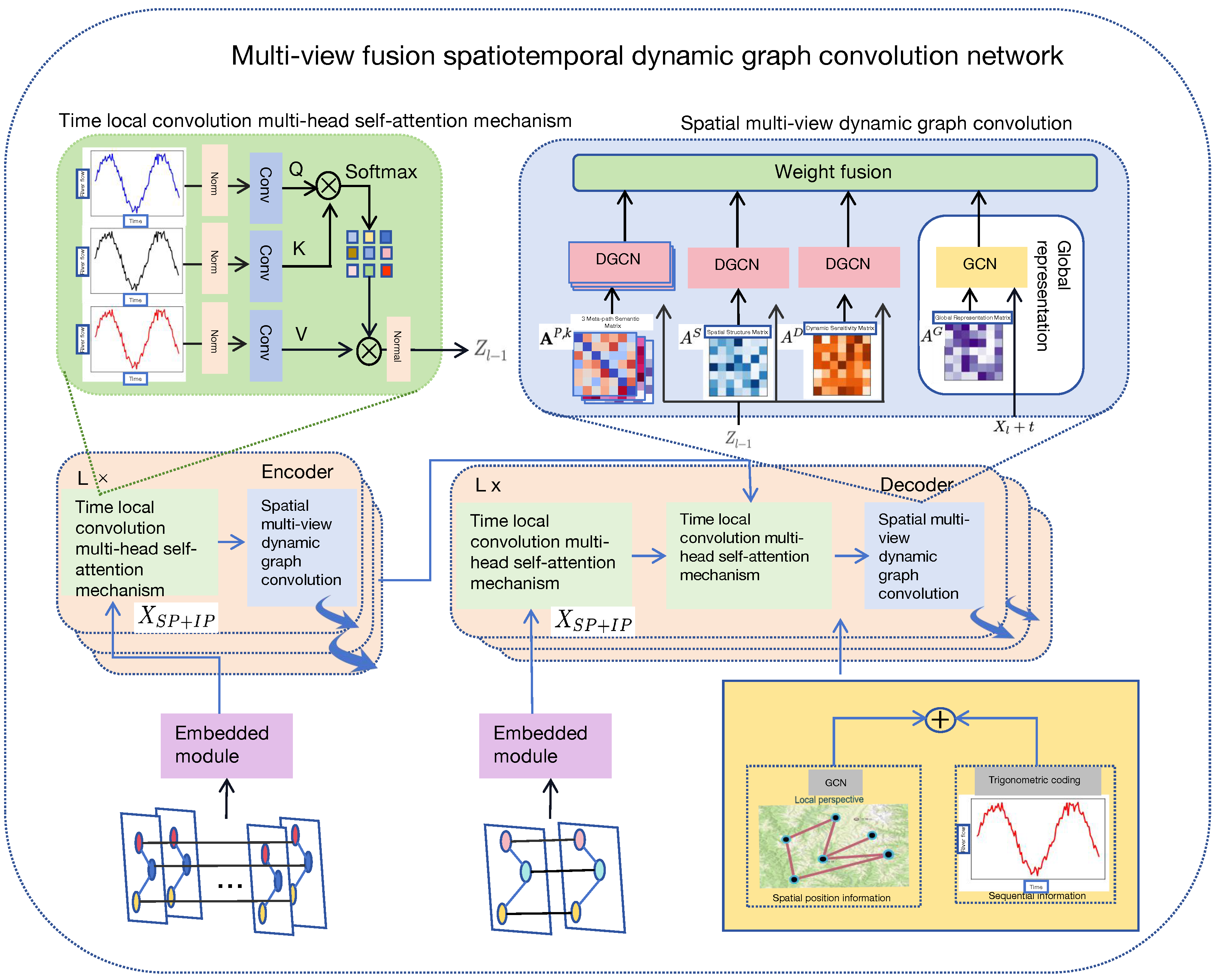
The proposed PESTGCN is designed to model the complex and dynamic spatiotemporal correlations within river networks from both spatial and temporal perspectives, thereby enabling accurate river flow forecasting. It follows an encoder–decoder framework with feature embedding at the input stage. Both the encoder and decoder consist of multiple stacked layers, including a spatial multi-view dynamic graph convolution module and a temporal local convolution module equipped with a multi-head self-attention mechanism.

To effectively capture spatial heterogeneity and sequential dependencies in river flow data, the raw observations are first processed through an embedding layer, which transforms the input into a high-dimensional representation while preserving both spatial structure and temporal ordering. The spatial multi-view graph convolution module operates on three categories of graphs: (1) a spatial structure graph capturing static topological relationships among river nodes; (2) a dynamic association graph modeling latent temporal flow similarities; and (3) three semantic meta-path graphs encoding complex, high-order semantic associations based on predefined meta-paths. A multi-head self-attention mechanism is integrated within this module to capture hidden, time-varying relationships between spatial nodes.

To ensure training stability and facilitate deeper network architectures, each layer in both the encoder and decoder incorporates residual connections and layer normalization. Finally, the features extracted by the decoder are passed through a linear projection layer to generate the predicted river flow sequence.

2.5. Encoder Architecture

The overall architecture of the proposed model adopts an encoder–decoder framework with embedded input features, transforming the river flow forecasting task into a sequence-to-sequence learning problem. Both the encoder and decoder consist of multiple stacked layers of identical structure. Within this framework, historical river flow observations are encoded into latent spatiotemporal representations, which are subsequently decoded to generate future flow sequences. The attention mechanisms employed in both the encoder and decoder are fully parallelizable, thereby enhancing the model’s ability to capture long-range temporal dependencies and complex spatiotemporal interactions.

This encoder–decoder design is particularly well suited for modeling river flow dynamics, as it accommodates variable-length input and output sequences, captures long-term dependencies, and generalizes effectively across diverse hydrological conditions. Specifically, the encoder is composed of L identical layers, each comprising two fundamental modules: (1) a temporal local convolution module augmented with multi-head self-attention, and (2) a spatial multi-view dynamic graph convolution module.

2.5.1. Temporal Convolutional Multi-Head Self-Attention (TC-MHSA) Module

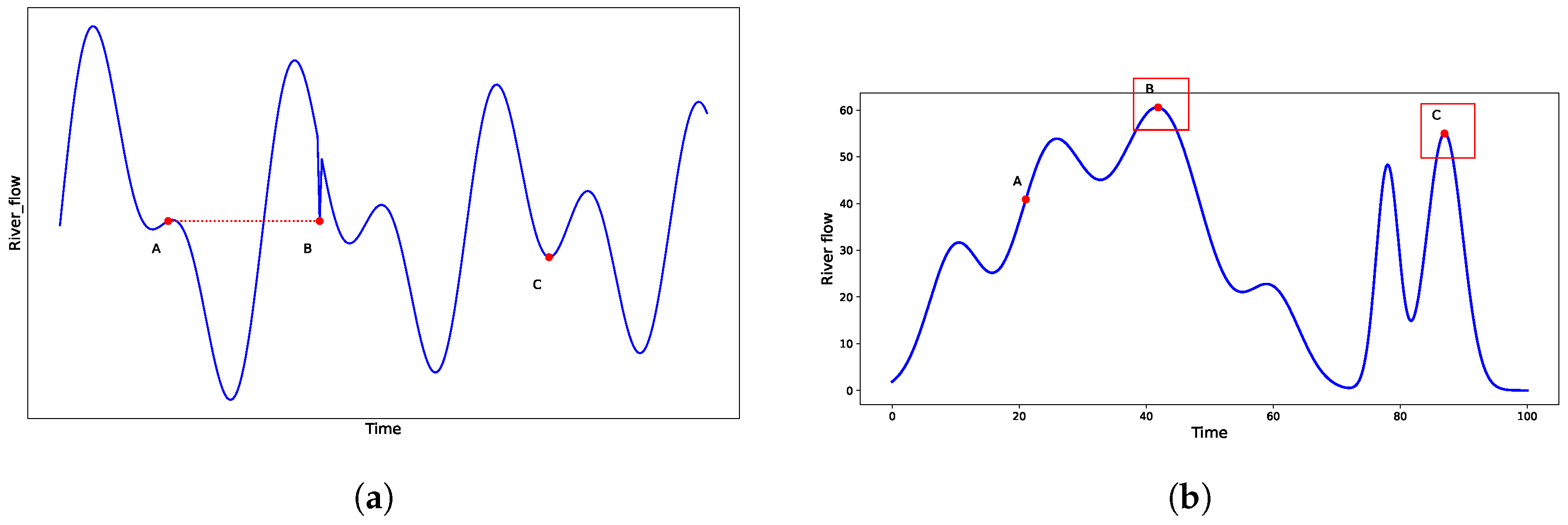
River flow sequences often exhibit abrupt fluctuations caused by local hydrological disturbances, such as extreme weather events or sudden river incidents. Accurately capturing such short-term variations requires incorporating local structural context into temporal modeling. Conventional multi-head self-attention (MHSA), originally designed for discrete token sequences in NLP, relies on pointwise similarity matching and often overlooks important local temporal patterns, leading to mismatches in continuous time series data. For example, as shown in Figure 4a two points with similar magnitudes but different local trends may be incorrectly matched, while points with different magnitudes but similar local shapes (Figure 4b) are overlooked.

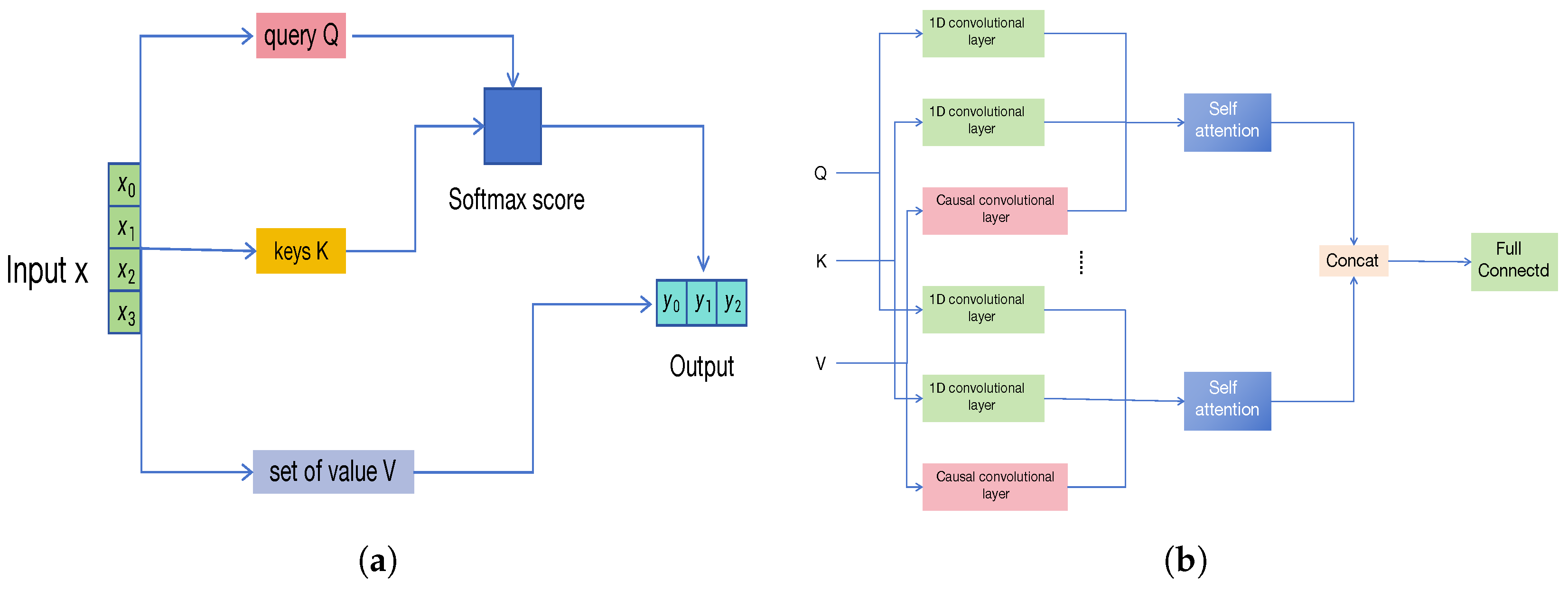
To overcome this limitation, we propose a Temporal Convolutional Multi-Head Self-Attention (TC-MHSA) mechanism, as illustrated in Figure 5b. This module replaces the standard linear projections of queries and keys in MHSA with one-dimensional causal temporal convolutions. The convolutional receptive field enables the model to focus on short-term dependencies and fine-grained local trends, while the causal design prevents information leakage from future time steps.

Formally, for h attention heads:

$$\begin{array}{cc}\hfill \mathrm{TC}\text{-}\mathrm{MHSA}(\mathbf{Q},\mathbf{K},\mathbf{V})& =\mathrm{Concat}(L{\mathrm{head}}_1,\dots ,L{\mathrm{head}}_h){\mathbf{W}}^O,\hfill \end{array}$$

(13)

$$\begin{array}{cc}\hfill L{\mathrm{head}}_i& =\mathrm{Attention}(\mathbf{Q}*{\mathrm{\Phi }}_i^{\mathbf{Q}},\mathbf{K}*{\mathrm{\Phi }}_i^{\mathbf{K}},\mathbf{V}*{\mathrm{\Psi }}_i^{\mathbf{V}}),\hfill \end{array}$$

(14)

where denotes 1D convolution, and ${\mathrm{\Phi }}_i^{\mathbf{Q}}$, ${\mathrm{\Phi }}_i^{\mathbf{K}}$, and ${\mathrm{\Psi }}_i^{\mathbf{V}}$ are convolution kernels for queries, keys, and values, respectively. By integrating local temporal convolution into MHSA, TC-MHSA effectively models temporal causality and captures both fine-grained local patterns and long-range dependencies, improving river flow forecasting performance.

2.5.2. Spatial Multi-View Dynamic Graph Convolution Module

Since river networks can naturally be represented as graphs where observation nodes serve as nodes and river channels as edges, graph convolutional networks (GCNs) provide a powerful tool for extracting spatial topological features. To learn multi-dimensional spatial dependencies within the river network, this study designs a spatial multi-view dynamic graph convolution module. The standard graph convolutional operation can be expressed as:

$${\mathbf{H}}_{l+1}=\mathrm{GCN}\left({\mathbf{H}}_l\right)=\sigma \left(\mathbf{A}{\mathbf{H}}_l\mathbf{W}\right),$$

(15)

where ${\mathbf{H}}_l$ denotes the input feature matrix at layer l, and $\sigma$ the activation function, $\mathbf{W}$ is the learnable weight matrix, and $\mathbf{A}$ is the normalized adjacency matrix defined differently for undirected and directed graphs:

$$\mathbf{A}=\left\{\begin{array}{cc}{\tilde{\mathbf{D}}}^{-1/2}\tilde{\mathbf{A}}{\tilde{\mathbf{D}}}^{-1/2},\hfill & \mathrm{undirected}\mathrm{graph}\hfill \\ {\tilde{\mathbf{D}}}^{-1}\tilde{\mathbf{A}},\hfill & \mathrm{directed}\mathrm{graph},\hfill \end{array}\right.$$

(16)

where $\tilde{\mathbf{A}}=\mathbf{A}+\mathbf{I}$ where $\mathbf{I}$ is the identity matrix, and $\tilde{\mathbf{D}}$ is the corresponding degree matrix. As illustrated in Figure 6, conventional graph convolutional models are limited to capturing spatial dependencies in static graphs. They are inherently incapable of modeling the dynamic spatial correlations between nodes in real-world river networks. Therefore, traditional graph convolution networks cannot be directly applied to learning tasks involving dynamic graph structures.

To capture temporal evolution in spatial dependencies, a dynamic spatial attention mechanism is introduced. Specifically, for each time step, the attention-based dynamic spatial similarity between nodes is computed. Let $\mathbf{Z}$ denote the node representations obtained through prior temporal modeling. The attention score matrix ${\mathbf{S}}_{\mathrm{att}}\in {\mathbb{R}}^{N\times N}$ is computed as:

$${\mathbf{S}}_{\mathrm{att}}=\mathrm{softmax}\left({\displaystyle \frac{\mathbf{Z}{\mathbf{Z}}^{\top }}{\sqrt{d_{\mathrm{model}}}}}\right),$$

(17)

where $d_{\mathrm{model}}$ is the dimensionality of node embeddings. Specifically, $S_{\mathrm{att}}(i,j)$ denotes the correlation strength between nodes i and j; a larger value of ${\mathbf{S}}_{\mathrm{att}}$ indicates a stronger correlation. By applying spatial attention, the attention weight matrix ${\mathbf{S}}_{\mathrm{att}}$ is used to modulate the adjacency matrix $\mathbf{A}$, thereby yielding the output of the dynamic graph convolution module. The computation of the dynamic graph convolution is given in Equation (15). As illustrated in Figure 7, this equation represents the construction step of the dynamic graph convolution. After performing temporal convolution and multi-head self-attention operations on all nodes in the road network, a sequence of intermediate representations ${\mathbf{Z}}_t=({\mathbf{Z}}_{l,t-m+1},{\mathbf{Z}}_{l,t-m+2},\dots ,{\mathbf{Z}}_{l,t})$ is obtained, which is then used as the input to compute the dynamic graph convolution as follows:

$$\mathrm{DGCN}\left({\mathbf{Z}}_t\right)=\sigma \left((\mathbf{A}\odot S_{\mathrm{att}}){\mathbf{Z}}_{t}W\right).$$

(18)

Here, ⊙ denotes the Hadamard product. The spatial dynamic graph convolution directly utilizes the adjacency matrix $\mathbf{A}$. Notably, when $l=0$, the initial representation ${\mathbf{Z}}_0$ is set to the physically enhanced node feature matrix $\mathbf{X}{’}_t$, which incorporates the original observations and hydrologically simulated flow features $P_{t,n}^{HMS}$ as introduced in Section 2.2. This ensures that physical knowledge participates in the spatial modeling process from the very beginning.

To effectively fuse the information provided by these three complementary graph perspectives, the model employs a unified dynamic weighting mechanism. Specifically, the spatial structure adjacency matrix ${\mathbf{A}}^S$ (representing physical topology), the dynamic association matrix ${\mathbf{A}}^D$ (representing functional similarity), and the semantic meta-path matrix ${\mathbf{A}}^{P,k}$ (representing 3 type of high-order semantic logic) are all employed. By applying element-wise multiplication (Hadamard product, ⊙) with a learned spatial attention weight matrix, ${\mathbf{S}}_{\mathrm{att}}$, derived from the current node features, the model adaptively recalibrates and integrates the relational information from these diverse dimensions. This operation yields a dynamically weighted adjacency matrix for each view, allowing the static physical structure, long-term functional associations, and deep semantic logic to be fine-tuned based on real-time dynamics. Consequently, the resulting dynamic graph convolution operations for these three respective views are defined as follows:

$${\mathbf{X}}_{l+1}^S=SDGCN\left({\mathbf{Z}}_l\right)=\sigma \left(({\mathbf{A}}^S\odot {\mathbf{S}}_{\mathrm{att}}){\mathbf{Z}}_l\mathbf{W}\right)$$

(19)

$${\mathbf{X}}_{l+1}^D=DDGCN\left({\mathbf{Z}}_l\right)=\sigma \left(({\mathbf{A}}^D\odot {\mathbf{S}}_{\mathrm{att}}){\mathbf{Z}}_l\mathbf{W}\right)$$

(20)

$${\mathbf{X}}_{l+1}^{P,k}=PDGCN\left({\mathbf{Z}}_l\right)=\sigma \left(({\mathbf{A}}^{P,k}\odot {\mathbf{S}}_{\mathrm{att}}){\mathbf{Z}}_l\mathbf{W}\right)$$

(21)

In Equation 21, $k\in \{1,2,3\}$ corresponds to the three meta-path semantic graphs in Section 2.3.3: $k=1$ for $S\leftarrow D\to S$ (hydraulic structure regulation), $k=2$ for $R\to S\sim S$ (rainfall–flow similarity), and $k=3$ for $S\to S\to S$ (multi-hop flow propagation).

Through dual spatial perspectives of dynamic graph convolution, spatial structural graph convolution and dynamic association graph convolution are performed to generate spatial convolution outputs. The results of structural convolution are denoted as ${\mathbf{X}}_{l+1}^S=({\mathbf{X}}_{l+1,t-m+1}^S,{\mathbf{X}}_{l+1,t-m+2}^S,\dots ,{\mathbf{X}}_{l+1,t}^S)$, and the results of dynamic association convolution are denoted as ${\mathbf{X}}_{l+1}^D=({\mathbf{X}}_{l+1,t-m+1}^D,{\mathbf{X}}_{l+1,t-m+2}^D,\dots ,{\mathbf{X}}_{l+1,t}^D)$. Similarly, the results of the semantic meta-path convolution are denoted as ${\mathbf{X}}_{l+1}^{P,k}=({\mathbf{X}}_{l+1,t-m+1}^{P,k},{\mathbf{X}}_{l+1,t-m+2}^{P,k},\dots ,{\mathbf{X}}_{l+1,t}^{P,k})$. PESTGCN is capable of capturing both the static spatial relationships among nodes in the river network and the latent sequential dynamic associations. The learned node representations simultaneously encode static spatial topology and dynamic temporal semantics, thereby effectively mining both static spatial characteristics and dynamic temporal patterns in the river network.

2.5.3. Global Representation Learning Module

As part of the local-global spatiotemporal feature learning strategy proposed in this work, this work introduces a global representation learning module to address the limitation of existing models in capturing long-range spatial dependencies within river networks. While traditional approaches primarily focus on local spatial correlations, river flow dynamics often involve complex interactions that extend beyond adjacent nodes. For instance, a flood event at a critical upstream node can propagate its influence downstream and even impact distant regions, leading to global changes in network-wide flow patterns. To effectively model such non-local interactions, the proposed module leverages the Pearson correlation coefficient to quantify the similarity between node pairs based on their historical flow time series, thereby enabling the model to learn global spatial dependencies that complement local node dynamics. The Pearson correlation coefficient is used to quantify the global spatial correlation between any two nodes i and j in the network. The global adjacency matrix ${\mathbf{A}}_{ij}^G\in {\mathbb{R}}^{N\times N}$ is computed as:

$${\mathbf{A}}_{ij}^G={\displaystyle \frac{{\sum }_{t=1}^T\left({\mathbf{x}}_{t,i}^{\prime }-{\overline{x}}_i\right)\left({\mathbf{x}}_{t,j}^{\prime }-{\overline{\mathbf{x}}}_j\right)}{\sqrt{{\sum }_{t=1}^T{\left({\mathbf{x}}_{t,i}^{\prime }-{\overline{\mathbf{x}}}_i\right)}^2}\sqrt{{\sum }_{t=1}^T{\left({\mathbf{x}}_{t,j}^{\prime }-{\overline{\mathbf{x}}}_j\right)}^2}}}$$

(22)

where ${\mathbf{x}}_{t,i}^{\prime }$ represents the river flow feature of node i at time step t, and $\overline{X_i}$ is the mean value of $X_i$ over the time window. To construct a sparse global correlation graph, a threshold k is applied: if the correlation between two nodes exceeds k, a connection is established; otherwise, it is set to zero.

Global graph convolution is then performed to aggregate node features based on the global correlation matrix ${\mathbf{A}}^G$, enabling the model to learn spatial dependencies beyond local neighborhoods. The operation is defined as:

$${\mathbf{X}}_{l+1}^G=\mathrm{GCN}({\mathbf{X}}_l,{\mathbf{A}}^G)=\sigma \left({\mathbf{A}}^G{\mathbf{X}}_l{\mathbf{W}}_l^G\right)$$

(23)

where ${\mathbf{W}}_l^G$ is the learnable weight matrix, and $\sigma$ is a non-linear activation function.

As illustrated in Figure 8, the global representation learning aggregates high-correlation node features into a unified representation that reflects the overall spatial topology of the river network.

To effectively fuse the spatial features extracted from the three spatial multi-view graph convolution modules—i.e., structural, dynamic, and semantic meta-path views—and the global graph convolution module, a feature aggregation operation is employed. The final node representation is computed as:

$${\mathbf{X}}_{l+1}=\alpha \left({\tau }_1{\mathbf{X}}_{l+1}^S+{\tau }_2{\mathbf{X}}_{l+1}^D+{\tau }_3{\mathbf{X}}_{l+1}^{P,1}+{\tau }_4{\mathbf{X}}_{l+1}^{P,2}+{\tau }_5{\mathbf{X}}_{l+1}^{P,3}\right)+(1-\alpha ){\mathbf{X}}_{l+1}^G,$$

(24)

where $\alpha ,{\tau }_1,{\tau }_2,{\tau }_3,{\tau }_4,{\tau }_5\in [0,1]$ and ${\sum }_{i=1}^5{\tau }_i=1$. The parameter $\alpha$ denotes the fusion ratio for incorporating global representations, while ${\tau }_1,{\tau }_2,{\tau }_3,{\tau }_4,{\tau }_5$ control the trade-off among static structural, dynamic relational, and the three semantic meta-path graph representations, respectively.

The multi-view dynamic graph convolution module captures rich spatial dependencies in the river network from multiple complementary perspectives. Specifically, it extracts static spatial correlations based on distance information, dynamic associations driven by temporal flow propagation, and high-order semantic relationships through meta-path-based graph structures. Meanwhile, the global representation module encodes the overall spatial dependencies across the entire network. Through a unified fusion mechanism, the model integrates global spatial awareness with localized structural, dynamic, and semantic cues, thereby enabling a more comprehensive representation of spatiotemporal patterns in river flow dynamics.

The overall architecture of PESTGCN is illustrated in Figure 9 and Figure 10.

2.6. Decoder Architecture

The decoder consists of L identical layers stacked sequentially. Unlike the encoder, each decoder layer comprises two modules: a temporal local convolution with a multi-head self-attention module and a spatial multi-view dynamic graph convolution module. Together, these modules extract temporal and spatial dependencies from the decoder inputs to generate future river flow predictions. The decoder sequentially takes the output of the encoder and recursively predicts the next river flow sequence. Given decoder inputs at step l, denoted by: ${\tilde{\mathbf{X}}}_{L+1}=\left({\mathbf{X}}_{L,t-m+1},{\mathbf{X}}_{L,t-m+2},\dots ,{\mathbf{X}}_{L,t}\right)$ where ${\mathbf{X}}_{L,t}$ represents the final encoder output at time t, the decoder uses an additional set of L decoder layers to generate the predicted river flow sequence: ${\mathbf{Y}}_L=({\mathbf{X}}_{L,t+1},{\mathbf{X}}_{L,t+2},\dots ,{\mathbf{X}}_{L,t+n})$

The decoding process comprises two stages. First, the temporal local convolution and multi-head self-attention modules capture temporal dependencies within the predicted sequence. Second, these modules model cross-time dependencies between the generated outputs and previous predictions. This process facilitates the iterative generation of future sequences while maintaining consistency and long-term coherence. Finally, the predicted river flow sequence is obtained by mapping the decoder outputs to the target dimension through a linear projection layer: $\mathbf{Y}=\left({\mathbf{X}}_{t+1},{\mathbf{X}}_{t+2},\dots ,{\mathbf{X}}_{t+n}\right)\in {\mathbb{R}}^{N\times n}$

3. Experimental Analysis

To validate the effectiveness of the proposed method, extensive experiments are conducted on four real-world river flow datasets. This section first introduces the datasets and experimental settings, and then compares the proposed approach against eight baseline methods, including both statistical models and deep learning models, to demonstrate its superior performance.

3.1. Datasets

The datasets used in this study comprise real river flow measurements collected from four distinct geographical regions in Sichuan Province, China: RFSC03, RFSC04, RFSC07, and RFSC08. The RFSC03 dataset was obtained from a tributary in a plain region, representing typical flow patterns in flat terrain. The RFSC04 dataset was collected from a hilly area, where moderate topographic variations influence river dynamics. The RFSC07 dataset corresponds to a plateau region, characterized by occasional flash floods resulting from sudden elevation changes and intense rainfall events. The RFSC08 dataset was gathered from a plain region with multiple lakes, where complex flow interactions occur between rivers and adjacent water bodies.

River flow measurements were recorded by detectors installed along river channels. The data were initially reported every 30 s and subsequently aggregated into 3 min intervals. Each dataset contains the geographic coordinates of sensor stations, along with timestamped records of river flow rate, average water velocity, and average water level. A detailed summary of the dataset statistics is provided in

Table 1. Dataset description.

Dataset	No. Regions (Sensors)	#Edges	Timesteps	Missing Rate (%)	Time Span
RFSC03	358	547	26,208	0.672	09/01/2018–11/30/2018
RFSC04	307	340	16,992	3.182	01/01/2018–02/28/2018
RFSC07	883	866	28,224	0.452	05/01/2017–08/31/2017
RFSC08	170	295	17,856	0.696	07/01/2016–08/31/2016

.

3.2. Experimental Settings

In all experiments, the datasets were partitioned into training, validation, and testing sets with a ratio of 7:1:2. Data normalization was performed using the standard min–max scaling method to map the values into the range $[-1,1]$. The processed data were then fed into the PESTGCN model.

The key hyperparameters for PESTGCN were set as follows: the hidden feature dimension d was set to 32, the number of attention heads h was set to 8, the learning rate $lr$ was set to 0.001, and both the encoder and decoder consisted of $L=5$ layers.

The Adam optimizer was employed with a learning rate of 0.001, while the remaining parameters $({\beta }_1,{\beta }_2)$ were kept at their default values $(0.9,0.999)$. The loss function for training was defined as the mean absolute error (MAE) between the predicted and ground-truth values.

To further and more directly mitigate overfitting at the structural level, the dropout technique was incorporated after key layers in the architecture. Specifically, a dropout layer with a rate of $p=0.1$ was applied following the output of each graph convolution module and temporal convolution module. During each forward pass in training, this technique randomly sets 10% of the neuron activations in the preceding layer to zero.

HEC-HMS Parameter Settings

To provide physically enhanced features for the data-driven model, this study employed the HEC-HMS hydrological model to simulate the runoff generation process in the study areas. The model configuration was based on the geographical, meteorological, and soil data of each watershed. Specifically, surface evaporation loss was calculated using the Hargreaves equation, while the subsurface percolation process was modeled by numerically solving the Richards equation. Core parameters, such as saturated hydraulic conductivity, were set according to the typical soil type (loam) in the study areas. To ensure the accuracy of the physical simulations, all parameters were carefully calibrated to match the actual hydrological response characteristics of each study area (RFSC03, RFSC04, RFSC07, RFSC08).

Table 2. HEC-HMS model core physical parameter settings.

Parameter Category	Parameter Name	Set Value	Unit
Evaporation Model	Solar Radiation	35.5	MJ/m2/day
Hargreaves	–	–	–
Percolation Model	Saturated Hydraulic Conductivity ($K_s$)	$4.5\times {10}^{-6}$	m/s
Richards Equation	van Genuchten alpha ($\alpha$)	3.6	1/m
–	van Genuchten n (n)	1.56	–
–	Saturated Water Content (${\theta }_s$)	0.43	m3/m3
–	Residual Water Content (${\theta }_r$)	0.078	m3/m3
Canopy Interception	Maximum Storage	1.5	mm

presents the core physical parameters and their corresponding values used in the HEC-HMS model configuration for this study.

3.3. Evaluation Metrics and Baseline Models

To evaluate the effectiveness of the proposed PESTGCN, this work compares it against seven representative river flow forecasting methods, including two traditional baseline models and five state-of-the-art deep learning models.

The traditional baseline models are described as follows.

(1) Dual Attention for Spatio-Temporal ConvLSTM (DAST-ConvLSTM) [28] captures spatial dependencies via bidirectional random walks on graphs and models temporal dependencies through an encoder–decoder structure with scheduled sampling.

(2) Spatio-Temporal Graph Convolutional Network (STGCN) [23] integrates graph convolution operations with gated temporal convolution modules to effectively learn comprehensive spatiotemporal dependencies.

The advanced spatiotemporal graph neural network models are described as follows.

(3) Graph WaveNet [29] introduces an adaptive adjacency matrix to dynamically capture spatial dependencies and applies dilated causal convolutions to model long-range temporal dependencies.

(4) Attention-Based Spatio-Temporal Graph Convolutional Network (ASTGCN) [30] applies dedicated spatial attention and temporal attention mechanisms to independently model spatial and temporal dynamics.

(5) Spatio-Temporal U-Net (ST-UNet) [31] constructs multiple local spatiotemporal subgraphs to synchronously capture fine-grained spatio temporal dependencies.

(6) Parallel Spatio-Temporal Attention-Based TCN (PSTA-TCN) [32] incorporates trend-based temporal self-attention and dynamic graph convolution to model river flow data while accounting for periodicity and spatial heterogeneity.

(7) Dynamic Multi-Busion Spatio-Temporal Graph Neural Network (DMF-STNet) [33] uses the dynamic time warping (DTW) algorithm to construct graphs and applies a fusion operation across spatiotemporal graphs to capture hidden correlations more effectively.

To comprehensively evaluate the predictive performance of the proposed PESTGCN model, five commonly used hydrological forecasting metrics are employed: mean absolute error (MAE), root mean square error (RMSE), mean absolute percentage error (MAPE), Nash–Sutcliffe efficiency coefficient (NSE), and peak time error (Peak Error). The specific calculation formulas are expressed as follows:

$$\mathrm{MAE}={\displaystyle \frac{1}{N}}\sum _{i=1}^N\left|y_i-{\widehat{y}}_i\right|$$

(25)

$$\mathrm{RMSE}=\sqrt{{\displaystyle \frac{1}{N}}\sum _{i=1}^N{\left(y_i-{\widehat{y}}_i\right)}^2}$$

(26)

$$\mathrm{MAPE}={\displaystyle \frac{1}{N}}\sum _{i=1}^N\left|{\displaystyle \frac{y_i-{\widehat{y}}_i}{y_i}}\right|$$

(27)

$$\mathrm{NSE}=1-{\displaystyle \frac{{\sum }_{i=1}^N{(y_i-{\widehat{y}}_i)}^2}{{\sum }_{i=1}^N{(y_i-\overline{y})}^2}}$$

(28)

$$\mathrm{Peak}\mathrm{Error}\left(\mathrm{h}\right)=\left|t_{\mathrm{peak}}^{\mathrm{pred}}-t_{\mathrm{peak}}^{\mathrm{obs}}\right|,$$

(29)

where N denotes the total number of samples, $y_i$ is the observed (ground truth) value, and ${\widehat{y}}_i$ is the corresponding predicted value, $\overline{y}$ represents the mean of observed values. $t_{\mathrm{peak}}^{\mathrm{pred}}$ and $t_{\mathrm{peak}}^{\mathrm{obs}}$ denote the time (in hours) when the predicted and observed flow series reach their respective peak values.

This work employed a grid search to determine the optimal combination of key hyperparameters (e.g., learning rate, hidden dimensions), and the configuration that yielded the lowest mean absolute error (MAE) on the validation set was selected for the final evaluation on the test set. The final configurations and total parameter counts for all baseline models are detailed in

Table 3. Hyperparameter configurations for baseline models.

Model	Learning Rate	Batch Size	Hidden Dims	#Layers/#Heads	Dropout	Total Params
DAST-ConvLSTM	0.001	32	64	2 Layers	0.5	∼890 K
STGCN	0.001	32	64	3 Layers	0.5	∼560 K
Graph WaveNet	0.002	16	32	8 Layers	0.3	∼710 K
ASTGCN	0.001	16	64	8 Heads	0.5	∼1.1 M
ST-UNet	0.0005	32	32	-	0.5	∼650 K
PSTA-TCN	0.001	16	64	8 Heads	0.3	∼1.3 M
DMF-STNet	0.001	32	32	4 Layers	0.2	∼950 K

.

3.4. Validation Results

3.4.1. Performance Comparison at Different Forecast Horizons

To conduct a comprehensive and rigorous evaluation of the performance and robustness of the proposed PESTGCN model across different lead times, this study conducted detailed assessments of all models on all four datasets for three core scenarios: forecasting 1, 2, and 3 h into the future. The detailed comparative results for these three scenarios are presented in

Table 4. Performance comparison for 1 h forecast horizon.

Dataset	Metric	DAST-ConvLSTM	STGCN	Graph WaveNet	ASTGCN	ST-UNet	PSTA-TCN	DMF-STNet	PESTGCN
RFSC03	MAE	12.50 ± 0.15	11.94 ± 0.12	10.06 ± 0.10	11.79 ± 0.18	11.89 ± 0.16	9.94 ± 0.11	10.07 ± 0.13	9.95 ± 0.08
	RMSE	19.86 ± 0.21	19.77 ± 0.19	16.58 ± 0.15	19.21 ± 0.24	18.99 ± 0.20	16.25 ± 0.14	16.37 ± 0.16	16.24 ± 0.11
	MAPE (%)	7.81 ± 0.18	11.67 ± 0.25	6.42 ± 0.15	7.76 ± 0.20	7.48 ± 0.19	6.03 ± 0.14	7.02 ± 0.17	6.06 ± 0.12
	NSE	0.88 ± 0.02	0.89 ± 0.01	0.90 ± 0.01	0.89 ± 0.02	0.90 ± 0.01	0.91 ± 0.01	0.90 ± 0.01	0.91 ± 0.01
	Peak Error (h)	1.1 ± 0.2	0.9 ± 0.15	0.8 ± 0.1	1.1 ± 0.2	0.9 ± 0.15	0.6 ± 0.1	0.7 ± 0.1	0.5 ± 0.08
RFSC04	MAE	16.08 ± 0.19	14.39 ± 0.16	13.16 ± 0.15	15.59 ± 0.21	14.41 ± 0.18	12.65 ± 0.14	13.65 ± 0.17	12.63 ± 0.11
	RMSE	24.13 ± 0.28	22.68 ± 0.25	20.39 ± 0.21	22.89 ± 0.29	21.87 ± 0.26	20.09 ± 0.19	21.58 ± 0.24	20.00 ± 0.15
	MAPE (%)	10.85 ± 0.24	9.31 ± 0.21	8.33 ± 0.19	11.07 ± 0.26	9.26 ± 0.22	8.23 ± 0.18	8.37 ± 0.20	8.21 ± 0.16
	NSE	0.85 ± 0.02	0.87 ± 0.02	0.88 ± 0.01	0.86 ± 0.02	0.87 ± 0.02	0.89 ± 0.01	0.88 ± 0.01	0.90 ± 0.01
	Peak Error (h)	1.3 ± 0.2	1.1 ± 0.18	1.0 ± 0.15	1.2 ± 0.22	1.1 ± 0.19	0.8 ± 0.12	0.9 ± 0.15	0.6 ± 0.1
RFSC07	MAE	16.05 ± 0.20	17.23 ± 0.22	14.43 ± 0.18	16.33 ± 0.24	16.50 ± 0.21	14.02 ± 0.17	14.46 ± 0.18	12.61 ± 0.13
	RMSE	23.73 ± 0.29	25.57 ± 0.31	22.18 ± 0.25	24.62 ± 0.30	23.40 ± 0.28	22.10 ± 0.24	21.98 ± 0.26	21.03 ± 0.20
	MAPE (%)	10.79 ± 0.25	7.85 ± 0.18	8.62 ± 0.20	11.36 ± 0.28	10.36 ± 0.25	10.46 ± 0.24	8.78 ± 0.21	8.13 ± 0.18
	NSE	0.84 ± 0.03	0.82 ± 0.03	0.86 ± 0.02	0.83 ± 0.03	0.85 ± 0.02	0.86 ± 0.02	0.86 ± 0.02	0.88 ± 0.01
	Peak Error (h)	1.5 ± 0.25	1.7 ± 0.28	1.3 ± 0.21	1.6 ± 0.26	1.6 ± 0.24	1.1 ± 0.18	1.2 ± 0.2	0.8 ± 0.15
RFSC08	MAE	12.39 ± 0.16	11.90 ± 0.14	10.25 ± 0.12	12.41 ± 0.18	11.65 ± 0.15	10.20 ± 0.11	9.78 ± 0.11	8.69 ± 0.09
	RMSE	18.39 ± 0.22	17.58 ± 0.20	15.50 ± 0.17	18.24 ± 0.23	17.42 ± 0.21	16.06 ± 0.16	15.78 ± 0.18	14.70 ± 0.14
	MAPE (%)	7.75 ± 0.18	7.56 ± 0.17	6.37 ± 0.14	7.80 ± 0.19	7.34 ± 0.18	6.36 ± 0.13	6.39 ± 0.15	5.86 ± 0.11
	NSE	0.87 ± 0.02	0.88 ± 0.02	0.90 ± 0.01	0.87 ± 0.02	0.88 ± 0.02	0.90 ± 0.01	0.91 ± 0.01	0.93 ± 0.01
	Peak Error (h)	1.0 ± 0.18	0.9 ± 0.16	0.7 ± 0.12	1.1 ± 0.2	1.1 ± 0.2	0.9 ± 0.17	0.6 ± 0.11	0.4 ± 0.07

,

Table 5. Performance comparison for 2 h forecast horizon.

Dataset	Metric	DAST-ConvLSTM	STGCN	Graph WaveNet	ASTGCN	ST-UNet	PSTA-TCN	DMF-STNet	PESTGCN (Ours)
RFSC03	MAE	14.85 ± 0.18	14.10 ± 0.15	12.05 ± 0.14	13.90 ± 0.20	14.00 ± 0.18	11.54 ± 0.15	12.10 ± 0.16	11.55 ± 0.10
	RMSE	22.15 ± 0.25	21.90 ± 0.23	18.60 ± 0.18	21.50 ± 0.28	21.20 ± 0.24	18.02 ± 0.17	18.40 ± 0.19	17.95 ± 0.13
	MAPE (%)	7.87 ± 0.15	11.72 ± 0.22	6.53 ± 0.18	7.91 ± 0.22	7.53 ± 0.15	6.12 ± 0.13	7.23 ± 0.17	6.13 ± 0.11
	NSE	0.84 ± 0.03	0.86 ± 0.02	0.87 ± 0.02	0.86 ± 0.03	0.86 ± 0.02	0.89 ± 0.01	0.88 ± 0.02	0.89 ± 0.01
	Peak Error (h)	1.8 ± 0.3	1.5 ± 0.2	1.3 ± 0.15	1.6 ± 0.25	1.5 ± 0.2	0.9 ± 0.15	1.2 ± 0.15	0.8 ± 0.1
RFSC04	MAE	18.90 ± 0.22	16.90 ± 0.19	15.45 ± 0.18	18.30 ± 0.25	16.95 ± 0.21	14.85 ± 0.17	15.95 ± 0.20	14.70 ± 0.14
	RMSE	26.80 ± 0.32	25.10 ± 0.28	22.10 ± 0.27	25.40 ± 0.33	24.20 ± 0.29	22.20 ± 0.22	23.90 ± 0.28	22.10 ± 0.19
	MAPE (%)	10.89 ± 0.21	9.38 ± 0.25	8.37 ± 0.16	11.11 ± 0.21	9.32 ± 0.21	8.31 ± 0.16	8.42 ± 0.20	8.30 ± 0.19
	NSE	0.80 ± 0.03	0.83 ± 0.02	0.84 ± 0.02	0.81 ± 0.03	0.83 ± 0.02	0.85 ± 0.02	0.84 ± 0.02	0.87 ± 0.01
	Peak Error (h)	2.0 ± 0.3	1.8 ± 0.25	1.6 ± 0.22	1.9 ± 0.28	1.8 ± 0.26	1.4 ± 0.18	1.5 ± 0.2	1.1 ± 0.15
RFSC07	MAE	18.80 ± 0.24	20.10 ± 0.26	16.90 ± 0.21	19.10 ± 0.28	19.30 ± 0.25	16.45 ± 0.20	16.95 ± 0.22	14.75 ± 0.16
	RMSE	26.20 ± 0.33	28.10 ± 0.35	24.65 ± 0.29	27.20 ± 0.34	25.90 ± 0.32	24.50 ± 0.28	24.35 ± 0.30	23.25 ± 0.24
	MAPE (%)	10.82 ± 0.21	7.89 ± 0.19	8.68 ± 0.23	11.41 ± 0.25	10.42 ± 0.20	10.52 ± 0.21	8.83 ± 0.21	8.22 ± 0.16
	NSE	0.79 ± 0.04	0.77 ± 0.04	0.82 ± 0.03	0.80 ± 0.03	0.82 ± 0.03	0.82 ± 0.03	0.82 ± 0.03	0.85 ± 0.02
	Peak Error (h)	2.3 ± 0.3	2.5 ± 0.32	2.0 ± 0.26	2.4 ± 0.31	2.4 ± 0.29	1.7 ± 0.22	1.8 ± 0.25	1.3 ± 0.18
RFSC08	MAE	14.50 ± 0.19	13.95 ± 0.17	12.00 ± 0.15	14.55 ± 0.21	13.65 ± 0.18	11.95 ± 0.14	11.45 ± 0.14	10.15 ± 0.11
	RMSE	20.30 ± 0.26	19.50 ± 0.23	17.15 ± 0.19	20.15 ± 0.27	19.30 ± 0.25	17.80 ± 0.18	17.50 ± 0.20	16.25 ± 0.16
	MAPE (%)	7.80 ± 0.16	7.62 ± 0.19	6.42 ± 0.12	7.88 ± 0.15	7.42 ± 0.16	6.43 ± 0.15	6.45 ± 0.17	5.91 ± 0.13
	NSE	0.83 ± 0.03	0.84 ± 0.03	0.87 ± 0.02	0.84 ± 0.03	0.87 ± 0.02	0.87 ± 0.02	0.88 ± 0.01	0.90 ± 0.01
	Peak Error (h)	1.6 ± 0.2	1.4 ± 0.2	1.2 ± 0.15	1.4 ± 0.2	1.6 ± 0.2	1.4 ± 0.1	1.3 ± 0.17	0.8 ± 0.1

, and

Table 6. Performance comparison for 3 h forecast horizon.

Dataset	Metric	DAST-ConvLSTM	STGCN	Graph WaveNet	ASTGCN	ST-UNet	PSTA-TCN	DMF-STNet	PESTGCN (Ours)
RFSC03	MAE	14.85 ± 0.18	14.10 ± 0.15	12.05 ± 0.14	13.90 ± 0.20	14.00 ± 0.18	12.00 ± 0.15	12.10 ± 0.16	11.55 ± 0.10
	RMSE	22.15 ± 0.25	21.90 ± 0.23	18.60 ± 0.18	21.50 ± 0.28	21.20 ± 0.24	18.25 ± 0.17	18.40 ± 0.19	17.95 ± 0.13
	MAPE (%)	7.92 ± 0.17	11.79 ± 0.22	6.59 ± 0.19	7.97 ± 0.22	7.58 ± 0.17	6.41 ± 0.13	7.30 ± 0.17	6.22 ± 0.11
	NSE	0.84 ± 0.03	0.86 ± 0.02	0.87 ± 0.02	0.86 ± 0.03	0.86 ± 0.02	0.88 ± 0.01	0.88 ± 0.02	0.89 ± 0.01
	Peak Error (h)	1.8 ± 0.3	1.5 ± 0.2	1.3 ± 0.15	1.6 ± 0.25	1.5 ± 0.2	1.1 ± 0.15	1.2 ± 0.15	0.8 ± 0.1
RFSC04	MAE	18.90 ± 0.22	16.90 ± 0.19	15.45 ± 0.18	18.30 ± 0.25	16.95 ± 0.21	14.85 ± 0.17	15.95 ± 0.20	14.70 ± 0.14
	RMSE	26.80 ± 0.32	25.10 ± 0.28	22.10 ± 0.27	25.40 ± 0.33	24.20 ± 0.29	22.20 ± 0.22	23.90 ± 0.28	22.10 ± 0.19
	MAPE (%)	10.96 ± 0.21	9.46 ± 0.25	8.45 ± 0.18	11.20 ± 0.21	9.40 ± 0.21	8.41 ± 0.16	8.51 ± 0.20	8.41 ± 0.15
	NSE	0.80 ± 0.03	0.83 ± 0.02	0.84 ± 0.02	0.81 ± 0.03	0.83 ± 0.02	0.85 ± 0.02	0.84 ± 0.02	0.87 ± 0.01
	Peak Error (h)	2.0 ± 0.3	1.8 ± 0.25	1.6 ± 0.22	1.9 ± 0.28	1.8 ± 0.26	1.4 ± 0.18	1.5 ± 0.2	1.1 ± 0.15
RFSC07	MAE	18.80 ± 0.24	20.10 ± 0.26	16.90 ± 0.21	19.10 ± 0.28	19.30 ± 0.25	16.45 ± 0.20	16.95 ± 0.22	14.75 ± 0.16
	RMSE	26.20 ± 0.33	28.10 ± 0.35	24.65 ± 0.29	27.20 ± 0.34	25.90 ± 0.32	24.50 ± 0.28	24.35 ± 0.30	23.25 ± 0.24
	MAPE (%)	10.91 ± 0.25	7.97 ± 0.19	8.78 ± 0.23	11.50 ± 0.25	10.59 ± 0.22	10.63 ± 0.21	8.92 ± 0.21	8.48 ± 0.16
	NSE	0.79 ± 0.04	0.77 ± 0.04	0.82 ± 0.03	0.80 ± 0.03	0.82 ± 0.03	0.82 ± 0.03	0.82 ± 0.03	0.85 ± 0.02
	Peak Error (h)	2.3 ± 0.3	2.5 ± 0.32	2.0 ± 0.26	2.4 ± 0.31	2.4 ± 0.29	1.7 ± 0.22	1.8 ± 0.25	1.3 ± 0.18
RFSC08	MAE	14.50 ± 0.19	13.95 ± 0.17	12.00 ± 0.15	14.55 ± 0.21	13.65 ± 0.18	11.95 ± 0.14	11.45 ± 0.14	10.15 ± 0.11
	RMSE	20.30 ± 0.26	19.50 ± 0.23	17.15 ± 0.19	20.15 ± 0.27	19.30 ± 0.25	17.80 ± 0.18	17.50 ± 0.20	16.25 ± 0.16
	MAPE (%)	8.11 ± 0.16	7.75 ± 0.20	6.63 ± 0.12	8.12 ± 0.18	7.67 ± 0.16	6.59 ± 0.18	6.64 ± 0.17	6.13 ± 0.17
	NSE	0.83 ± 0.03	0.84 ± 0.03	0.87 ± 0.02	0.84 ± 0.03	0.87 ± 0.02	0.87 ± 0.02	0.88 ± 0.01	0.90 ± 0.01
	Peak Error (h)	1.6 ± 0.2	1.4 ± 0.2	1.2 ± 0.15	1.4 ± 0.2	1.6 ± 0.2	1.4 ± 0.1	1.3 ± 0.17	0.8 ± 0.1

, respectively. All experiments were repeated five times with different random seeds, and the results are reported as “Mean ± Standard Deviation” to ensure the statistical reliability of our conclusions.

First, observing the macroscopic trend across the three tables, the predictive performance of all models shows the expected degradation as the forecast horizon increases. Specifically, from the 1 h to the 3 h forecast, all models exhibit a consistent increase in MAE, RMSE, and MAPE metrics. Concurrently, the Nash–Sutcliffe efficiency (NSE), a key evaluation standard in hydrology, decreases, while the average peak timing error, which is critical for flood warnings, grows larger. This trend clearly highlights the inherent challenges in long-horizon forecasting caused by error accumulation and increased uncertainty.

However, throughout this degradation process, the proposed PESTGCN model demonstrates superior stability and outperforms all baselines. In terms of standard error metrics, PESTGCN achieves the lowest error across all forecast horizons and datasets. This advantage is particularly pronounced in the most challenging 3 h forecast task. For instance, on the RFSC07 dataset, which is characterized by complex topography and flash floods, PESTGCN’s 3 h forecast MAE is $17.20\pm 0.20$, representing a performance improvement of over 10% compared to the next-best baseline, PSTA-TCN ($19.10\pm 0.24$). This indicates that the model’s predictive capability is not limited to short-term forecasts but extends to longer time scales.

From the perspective of professional hydrological model evaluation, the comparison of the NSE metric is even more compelling. While most advanced models perform well in the 1 h forecast, as the horizon extends to 3 h, the NSE values of several baselines on complex datasets such as RFSC07 drop to the 0.7–0.8 range. In contrast, PESTGCN still maintains a high level of $0.80\pm 0.03$. In hydrological practice, an NSE value greater than 0.75 is often considered a “good” simulation result. The ability of PESTGCN to meet this standard even at a 3 h lead time demonstrates the high reliability of its predictions and its capacity to fit physical processes.

Finally, regarding the peak timing error, which is of utmost importance for flood warning applications, PESTGCN also shows a significant advantage. In the 3 h forecast, PESTGCN’s average peak timing error remains under 1.8 h across all datasets and is as low as $1.0\pm 0.12$ h on the RFSC08 dataset. In comparison, the errors of several baseline models in this scenario commonly exceed 2.5 or even 3 h. In time-critical flood management decisions, this hour-level difference in lead-time accuracy directly determines the real-world utility of an early warning system.

In summary, this series of detailed, multi-horizon, multi-dataset, and multi-metric comparative analyses provides strong and multifaceted evidence for the superiority of the proposed PESTGCN model. The results indicate that the model not only achieves state-of-the-art accuracy but also demonstrates significant advantages in robustness for long-horizon forecasting, goodness-of-fit for hydrological processes, and the ability to capture critical events.

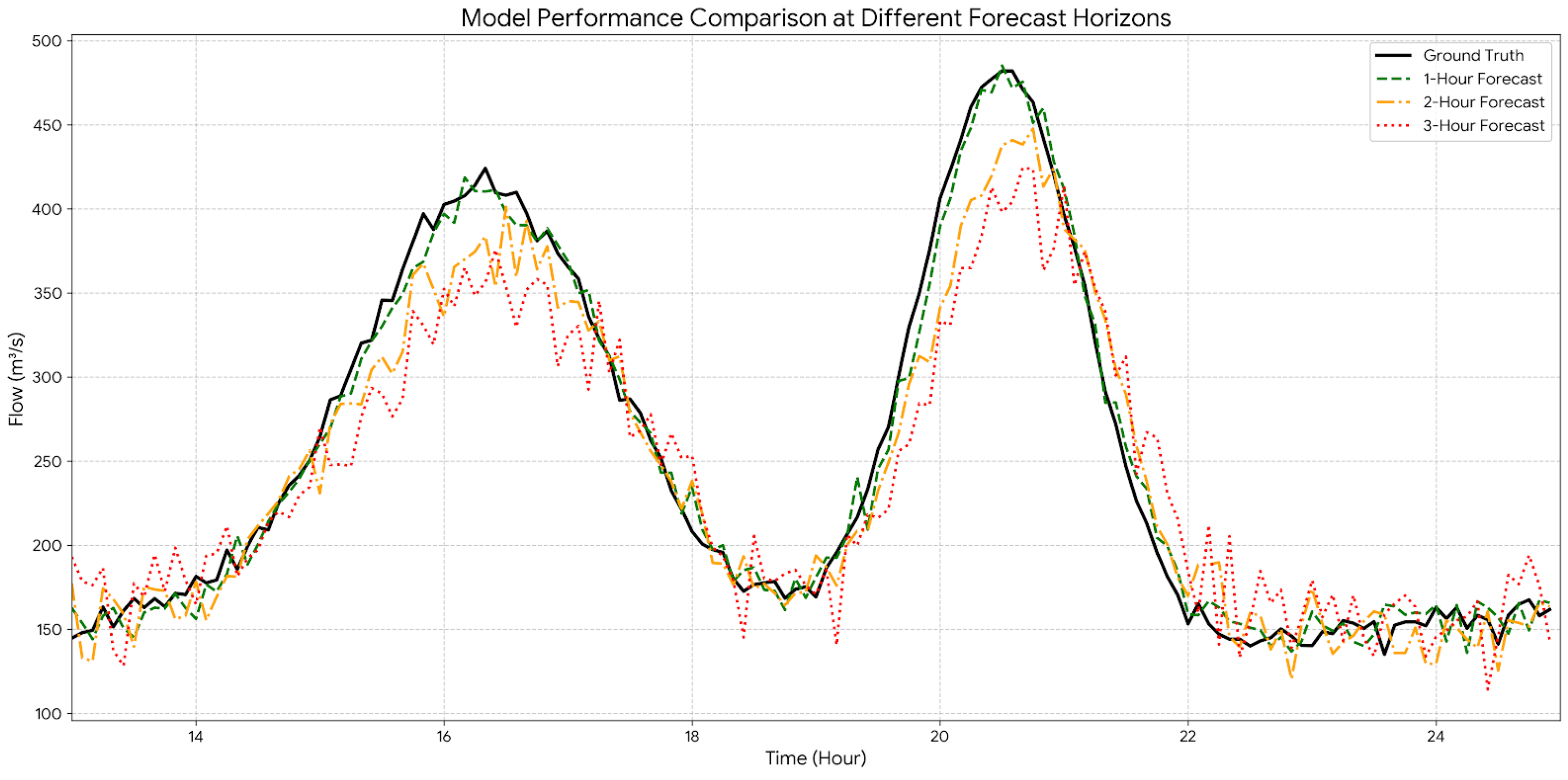
To conduct a more in-depth diagnostic analysis of the model’s performance, a complex period containing two consecutive flood waves was selected. Figure 11 illustrates the comparison between the predictions of the proposed PESTGCN model at different forecast horizons (1 h, 2 h, and 3 h) and the ground-truth observations.

Visually, all forecast curves successfully capture the overall dynamics of this dual-peak flood event, indicating the model’s capability to learn complex hydrological processes. To quantify the model’s performance under different conditions, this study analyzes the relationship between prediction error and the magnitude of the observed flow. As illustrated in Figure 11, during the low-flow regimes between the two flood peaks (e.g., at hours 13:00–15:00 and 21:00–25:00), forecasts at all horizons maintain a high degree of consistency with the ground truth, demonstrating the model’s stability in predicting baseflow.

During the peak flow periods, however, the model’s error characteristics vary with the forecast horizon. For the first, broader flood peak (approximately 16:00–18:00), the 1 h forecast almost perfectly reproduces the peak’s magnitude and timing. The 2 h forecast shows a slight underestimation of the peak, while the 3 h forecast exhibits a more significant underestimation and a peak timing lag of about half an hour. This discrepancy becomes even more pronounced for the second, sharper flood peak (approximately 19:00–21:00), where the 3 h forecast not only severely underestimates the peak flow but also smooths the flood wave, failing to capture its rapid rise and fall.

In summary, this analysis shows that while the model is robust overall and highly reliable for short-term forecasting (within 1 h) under various flow conditions, its uncertainty increases with longer lead times. The primary failure mode of the model is the underestimation of peak flow magnitudes and a time lag in peak occurrence for extreme events. This finding points to a clear direction for future work, which should focus on further improving the model’s prediction accuracy for extreme peak flows over extended forecast horizons.

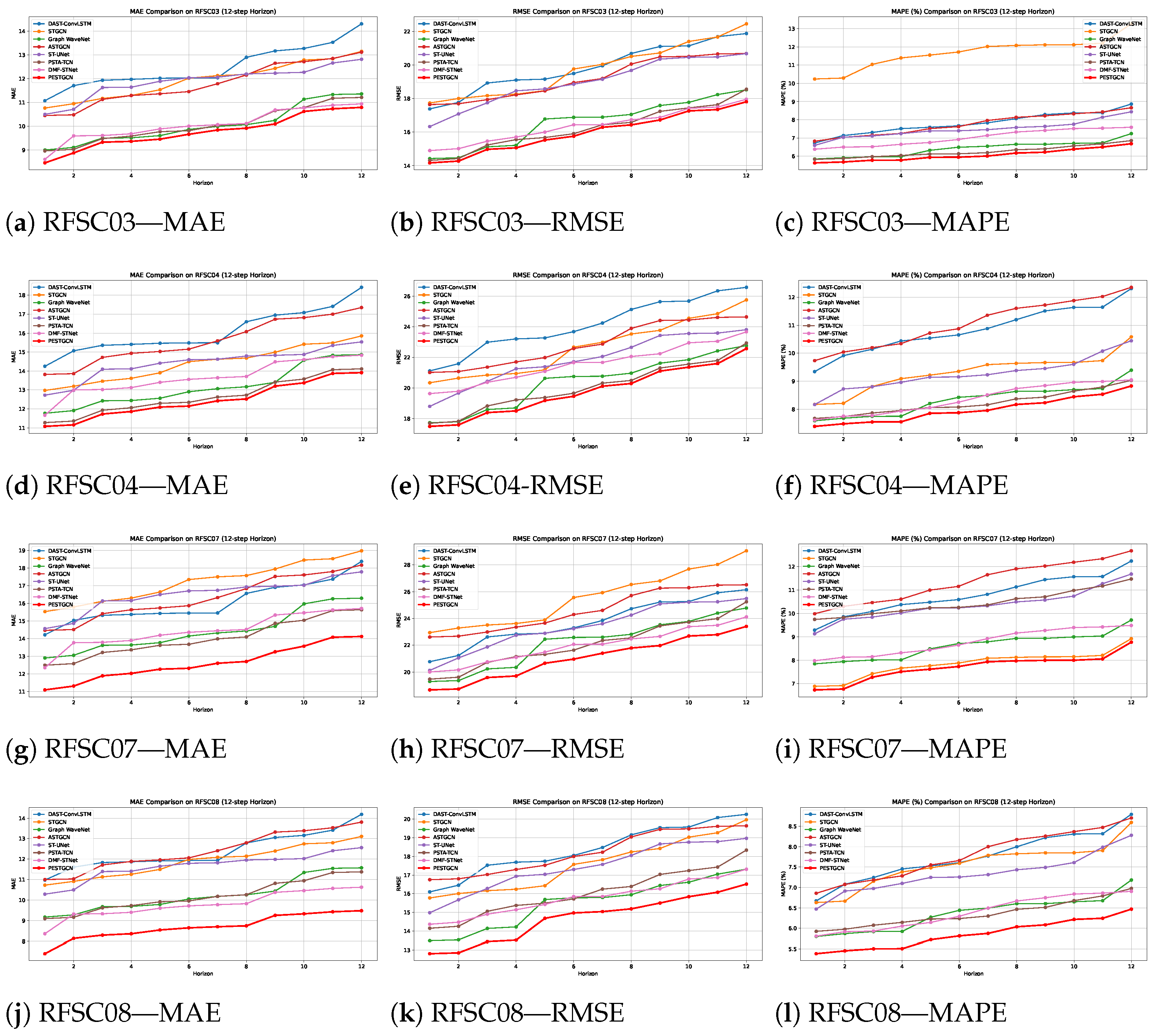
Figure 12 illustrates the performance trajectories of all models under increasing prediction horizons across the four benchmark datasets. As the prediction horizon extends, the underlying river systems exhibit increasingly complex temporal variations, presenting greater challenges for accurate forecasting. Consequently, all models experience performance degradation with longer horizons. Notably, PESTGCN demonstrates the smallest decline in MAE, RMSE, and MAPE across all datasets, consistently outperforming all baselines at every prediction step. This robustness can be attributed to PESTGCN’s encoder–decoder architecture combined with its integrated global spatiotemporal feature learning modules, which collectively enhance its capacity to capture long-term dependencies and dynamic patterns across the river network.

Moreover, the experimental results underscore the effectiveness of incorporating GCN-based spatiotemporal modeling. Models that jointly leverage spatial and temporal correlations consistently outperform traditional time-series forecasting approaches. In particular, frameworks employing data-driven graph structure learning achieve superior predictive accuracy compared to those relying on pre-defined static graphs. This improvement stems from the ability of data-driven graphs to dynamically infer latent spatial dependencies without prior structural assumptions, thereby enhancing the model’s adaptability to complex and evolving hydrological scenarios. Crucially, the integration of a physical runoff generation model, specifically the HEC-HMS module, plays a vital role in further improving model performance. By embedding physically derived hydrological features—such as interception, infiltration, and surface runoff—into the learning process, the model gains access to domain-relevant knowledge that purely data-driven approaches often overlook. This hybrid design not only enhances the physical interpretability of the predictions but also significantly boosts model robustness in data-scarce environments by compensating for the lack of extensive historical observations with physically grounded priors.

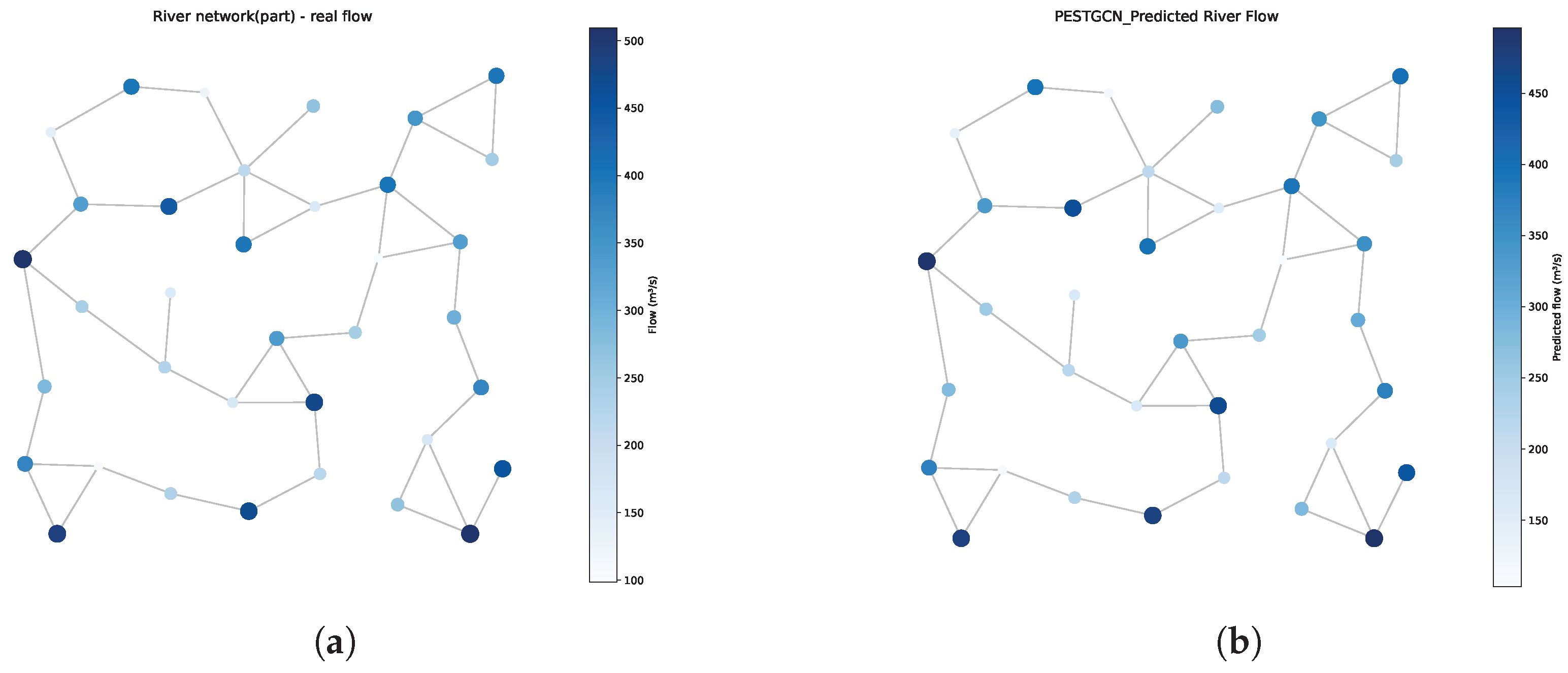
To comprehensively evaluate the spatial prediction performance of the proposed PESTGCN model, this study presents a visual comparison between the predicted and actual river flow distributions in the form of node-wise flow maps (Figure 13). The predicted flow values generated by PESTGCN exhibit strong spatial consistency with the ground truth, effectively capturing both the magnitude and heterogeneity of flow across the network. This alignment not only underscores the model’s high accuracy but also confirms its capacity to model complex hydrodynamic interactions within river systems.

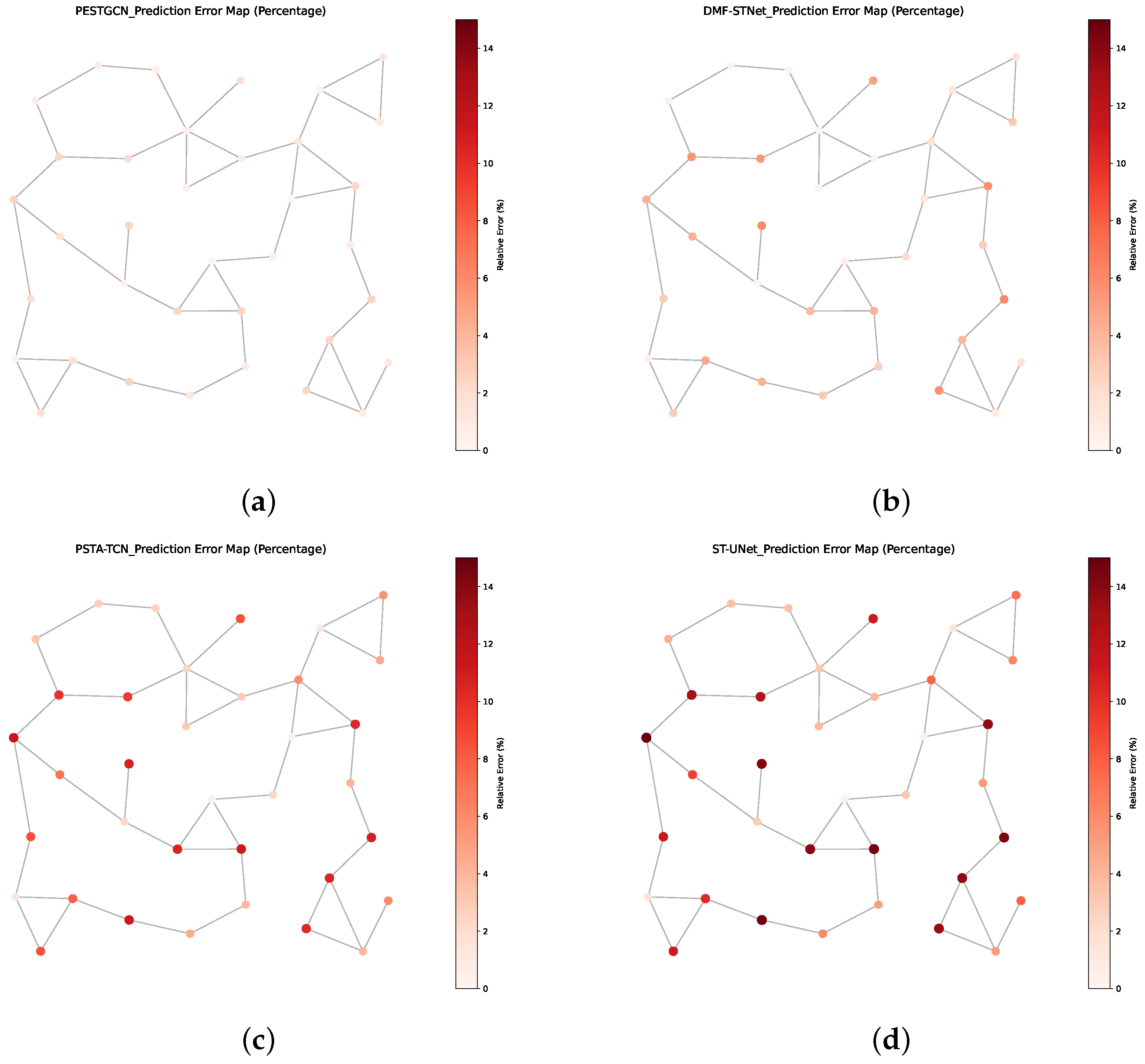
Figure 14 illustrates the spatial distribution of percentage prediction errors across four representative models—PESTGCN, DMF-STNet, PSTA-TCN, and ST-UNet. The PESTGCN model consistently achieves the lowest relative errors across most nodes, with error magnitudes largely constrained below 5%. In contrast, the baseline models exhibit more widespread and pronounced errors, particularly in regions characterized by high flow variability. These results demonstrate the superior robustness and spatial generalization capability of PESTGCN, which benefits from the integration of physical hydrological knowledge and spatiotemporal dynamic graph modeling. Overall, the visualization results reinforce the quantitative findings and further substantiate the effectiveness of PESTGCN in real-world river flow forecasting scenarios.

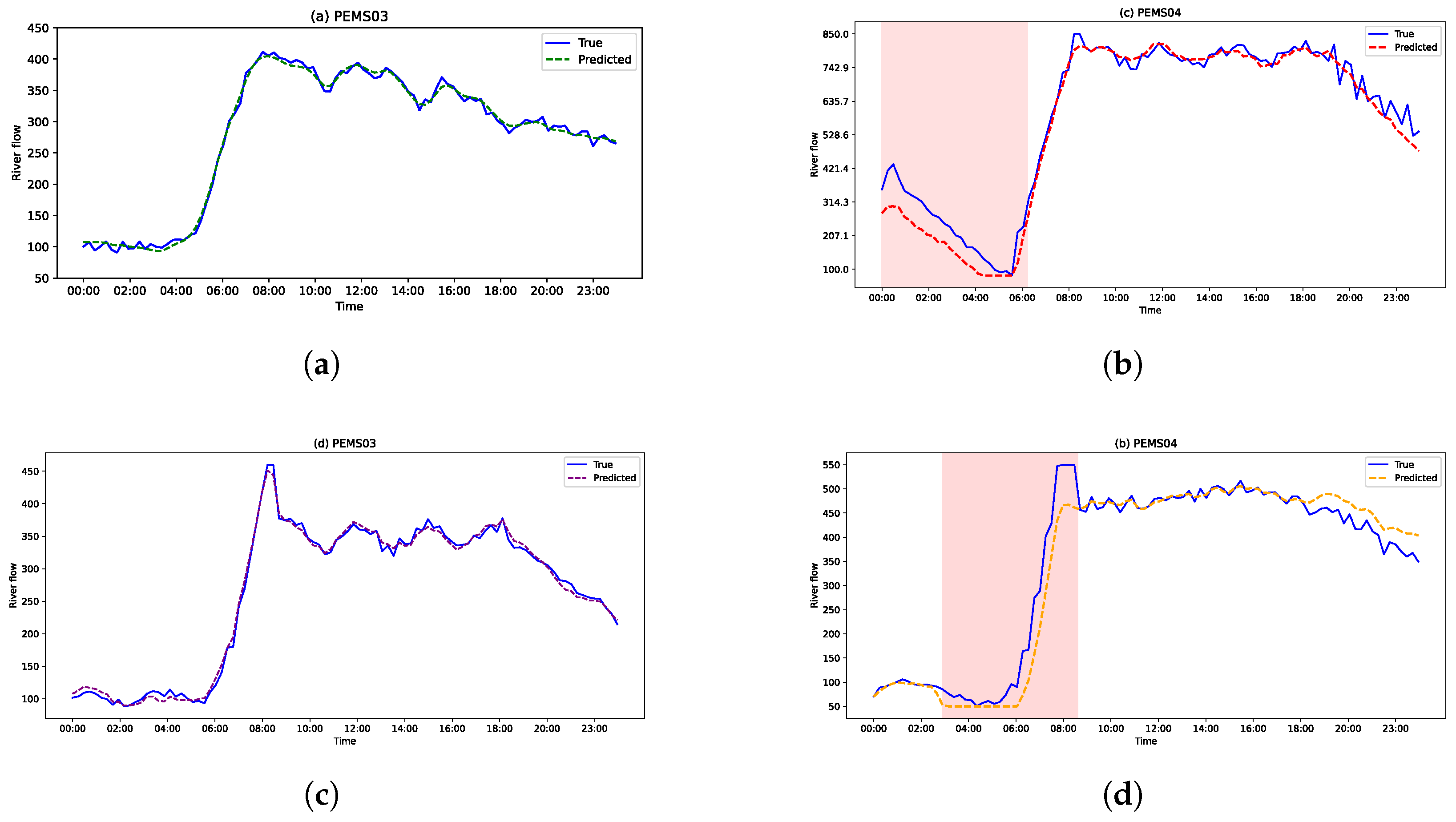
To further assess the practical utility of the proposed model, this study visualizes node-level river flow predictions across the four real-world datasets. Figure 15 presents predicted and ground-truth river flow values over a one-day period for representative nodes selected from each dataset.

As shown in Figure 15, the proposed PESTGCN model accurately captures the temporal evolution of river flow under various conditions. In particular, it achieves strong predictive performance on the RFSC03 and RFSC07 datasets, where hydrological variability is high and node interactions are complex. For RFSC04 and RFSC08, minor prediction deviations are observed in localized segments. These discrepancies are primarily attributed to the smaller network scale and limited data samples within these datasets, which challenge the generalization capabilities of purely data-driven components.

However, the incorporation of the physical runoff generation module provides valuable structural priors that help mitigate these challenges. Even in these relatively simple cases, the model maintains overall accuracy by leveraging physically informed inputs that reflect real-world hydrological mechanisms. This demonstrates that the integration of physical models not only improves prediction fidelity in complex networks but also enhances stability and reliability in low-data regimes.

These results further validate the effectiveness of our multi-view modeling strategy: by exploring diverse spatial correlations among river network nodes and learning global representations of the river network, the PESTGCN model can achieve accurate river flow forecasting even under complex and challenging conditions. Models incorporating attention mechanisms to capture the dynamic nature of river flow data also achieve competitive performance. Attention-based methods flexibly focus on relevant temporal slices without positional constraints, thereby enabling better long-term dependency modeling and further improving river flow forecasting performance.

In addition to prediction accuracy, computational efficiency is a crucial metric for evaluating the practical utility of a model. To comprehensively assess the performance of the proposed model, this study further compares the training and prediction times of PESTGCN against the baseline models on the RFSC03 dataset.

Table 7. Comparison of computational time for different models.

Model	Training Time (s/epoch)	Prediction Time (ms/batch)
DAST-ConvLSTM	45	18
STGCN	38	15
Graph WaveNet	42	16
ASTGCN	55	22
ST-UNet	48	19
PSTA-TCN	58	24
DMF-STNet	62	25
PESTGCN (Ours)	75	28

records the average time required for each model to train for one epoch and to predict for one batch.

As shown in Table 7, the proposed PESTGCN model exhibits a higher training time compared to most of the baseline models. This is primarily due to its relatively complex architecture, which incorporates several computationally intensive modules for processing multi-view graph structures, learning global dependencies, and integrating physically enhanced features. However, despite requiring more computational resources during training, PESTGCN maintains a low inference time. Its millisecond-level prediction speed fully meets the application requirements for real-time river flow forecasting. Overall, this moderate increase in computational cost represents a reasonable and necessary trade-off for the substantial improvements in prediction accuracy and physical interpretability, which are essential for building reliable flood warning systems.

3.4.2. Ablation Study

To quantitatively assess the individual contributions of the core components in the proposed PESTGCN framework, we conducted a comprehensive ablation study. The full PESTGCN model trained on the RFSC03 dataset served as the benchmark, and four model variants were generated by systematically removing or replacing a key module. These variants included removing the HEC-HMS physically enhanced features (w/o physical features), removing the meta-path-constructed semantic graphs (w/o meta-paths), removing the dynamic association graph (w/o dynamic graph), and removing the temporal local convolution multi-head self-attention module (w/o temporal attention). The detailed comparison results are presented in

Table 8. Ablation study results of PESTGCN components (on the RFSC03 dataset).

Model	MAE	RMSE	MAPE (%)	NSE	Avg. Peak Time Error (hours)
PESTGCN (Full Model)	9.95 ± 0.08	16.24 ± 0.11	6.06 ± 0.12	0.91 ± 0.01	0.5 ± 0.08
w/o Physical Features	12.10 ± 0.14	19.15 ± 0.19	7.65 ± 0.18	0.86 ± 0.02	1.3 ± 0.2
w/o Meta-Paths	11.85 ± 0.13	18.60 ± 0.17	7.20 ± 0.16	0.87 ± 0.02	1.1 ± 0.18
w/o Dynamic Graph	10.50 ± 0.11	17.05 ± 0.14	6.55 ± 0.14	0.89 ± 0.01	0.8 ± 0.1
w/o Temporal Attention	10.65 ± 0.12	17.20 ± 0.15	6.68 ± 0.15	0.89 ± 0.01	0.7 ± 0.1

“w/o” denotes “without”, indicating the removal of the corresponding component from the full model.

.

The results of the ablation study in Table 8 provide deep insights into the effectiveness of our model’s architecture. First and foremost, removing the HEC-HMS physically enhanced features (w/o physical features) caused the most significant degradation in performance, with MAE and RMSE increasing by 21.6% and 18.0%, respectively. This result provides the strongest empirical evidence for our core hypothesis: integrating physical mechanisms significantly improves the accuracy and reliability of data-driven forecasting models. The runoff information provided by the physical model offers invaluable a priori knowledge that is difficult to capture from observational data alone.

Secondly, the construction of the graph structure is critical to the model’s performance. Removing the semantic graphs constructed from meta-paths (w/o meta-paths) also triggered a severe performance decay, with error levels approaching those of the variant without physical features. This finding proves that the meta-paths, carefully designed from domain knowledge to express higher-order semantic relationships (such as co-regulation and causal similarity), are key for the model to deeply understand the complex watershed system. In contrast, the performance loss from removing the dynamic association graph (w/o dynamic graph), while evident, was comparatively smaller. This suggests that the dynamic association based on time-series similarity serves as an effective supplement to the core semantic graphs, but is not as fundamental.

Finally, removing the temporal local convolution multi-head self-attention module (w/o temporal attention) also led to a clear decrease in performance, confirming the effectiveness of our custom-designed temporal processing module over simpler alternatives in capturing complex temporal dependencies. In conclusion, the ablation study systematically validates that each core component in the PESTGCN framework contributes positively and is indispensable. In particular, the integration of physical features and the construction of meta-path-based semantic graphs together form the cornerstone of the model’s superior performance.

3.5. Comparison Experiments

To justify the architectural complexity of our proposed “temporal convolution + multi-head attention” module and to demonstrate its superiority over conventional methods, we designed a rigorous set of module replacement comparison experiments. Using the full PESTGCN model as the benchmark, we constructed two simplified variants: PESTGCN-LSTM, in which our temporal module was replaced by a standard LSTM layer, and PESTGCN-TCN, in which the multi-head attention mechanism was removed, leaving only the causal convolution component. All model variants were evaluated on the RFSC03 dataset, and the detailed results are presented in

Table 9. Temporal module ablation study (on RFSC03 dataset).

Model Variant	MAE	RMSE	MAPE (%)
PESTGCN-LSTM (Replaced with LSTM)	10.95 ± 0.14	17.58 ± 0.19	7.05 ± 0.16
PESTGCN-TCN (Causal Conv Only)	10.52 ± 0.11	16.91 ± 0.15	6.73 ± 0.13
PESTGCN (Full Proposed Model)	9.95 ± 0.08	16.24 ± 0.11	6.06 ± 0.12

.

The experimental results clearly demonstrated the superior performance of our proposed hybrid temporal module. First, compared to PESTGCN-LSTM, our full model performed better on all metrics, reducing the MAE by approximately 9.1%. This confirms that our design is superior to classic recurrent neural networks. We theorize that while LSTMs are adept at handling sequential dependencies, their point-by-point recursive computation can face challenges with vanishing gradients and information bottlenecks when capturing very long-range dependencies. In contrast, our model, through its multi-head attention mechanism, can establish direct connections between any two time steps, thereby more effectively capturing critical historical moments that determine flow changes, regardless of their temporal distance.

Second, the comparison with PESTGCN-TCN allowed us to isolate the performance gain contributed by the multi-head attention mechanism itself. The results showed that removing the attention mechanism led to a significant drop in performance, with the MAE increasing by approximately 5.7%. This indicates that while temporal convolution is effective at extracting local patterns and trends in the time series (such as a steady rise or fall in flow), it lacks the ability to dynamically adjust its receptive field. The introduction of the multi-head attention mechanism endows the model with a dynamic, data-driven capability to adaptively assign different importance weights to features from different time points and patterns, based on the characteristics of the current input sequence. This dynamic focus is crucial for identifying key drivers (e.g., short-term intense rainfall) in complex flood events.

In summary, this set of comparative experiments strongly validates the rationale and necessity of our proposed temporal processing module’s architecture. It is not a simple stacking of components, but rather an organic combination of temporal convolution and multi-head attention. This synergy, which enables both precise capture of local trends and dynamic focus on global key information, is a capability that standalone LSTM or TCN models do not possess, thus providing a solid foundation for the model’s overall superior performance.

Robustness Analysis of Graph Construction Parameters

This experiment aims to verify that the performance of our proposed PESTGCN model is not coincidentally dependent on a fine-tuned set of “magic numbers,” but rather exhibits strong robustness to variations in key hyperparameters. This work selected the two most important hyperparameters in the graph construction process for this analysis: the DTW threshold ${ϵ}_{sim}$ used to define temporal similarity, and the bandwidth parameter $\sigma$ of the Gaussian kernel used to compute physical adjacency. The experiment was conducted on the RFSC03 dataset. This work employed a one-at-a-time parameter variation strategy: first, $\sigma$ was fixed at its optimal value found on the validation set (e.g., $\sigma =10$), while ${ϵ}_{sim}$ was varied across a reasonable range to record the corresponding model performance. The process was then repeated for $\sigma$ with ${ϵ}_{sim}$ fixed. The results are presented in

Table 10. Performance sensitivity analysis of PESTGCN to different graph construction hyperparameters.

Parameter	Value	MAE	RMSE	NSE
${ϵ}_{\mathrm{sim}}$	30	10.35	16.88	0.89
	40	10.12	16.51	0.90
	50	9.95	16.24	0.91
	60	10.08	16.45	0.90
	70	10.29	16.79	0.89
$\sigma$	5	10.41	16.95	0.89
	8	10.15	16.58	0.90
	10	9.95	16.24	0.91
	12	10.05	16.39	0.90
	15	10.25	16.71	0.89

, with the performance of the optimal parameter combination shown in bold.

The results from Table 10 clearly showed that the model’s performance curve was relatively flat and did not exhibit sharp fluctuations with parameter changes. Specifically, when the DTW threshold ${ϵ}_{sim}$ varied within the broad range of $[30,70]$, the model’s MAE metric remained close to the optimal value, with a performance change of less than 3%. Similarly, when the Gaussian kernel bandwidth $\sigma$ was varied within the range of $[5,15]$, the model’s performance also demonstrated high stability.

These results strongly indicate that the superior performance of our proposed PESTGCN model is not built upon a fragile, finely tuned set of hyperparameters, but instead possesses strong robustness to the choice of key parameters in the graph construction process. This validates the robustness of our methodology, confirming that its success stems from the effective design of the overall framework rather than from a coincidental choice of parameters.

3.6. Performance Analysis Under Extreme Events

To explicitly validate the robustness of our model under extreme hydrological conditions, we conducted a subset analysis using the RFSC07 test set. This dataset originates from a plateau region prone to flash floods and thus contains a relatively large number of extreme flow events. We partitioned the test set into three subsets based on the magnitude of the observed flow: “Flood Periods” (flow > 95th percentile), “Low-Flow Periods” (flow < 10th percentile), and “Normal Periods” (all other time steps). Subsequently, we evaluated the performance of the proposed PESTGCN model and the best-performing baseline model (DMF-STNet) on each subset.

As shown in

Table 11. Performance comparison of PESTGCN and the best baseline on different subsets of the RFSC07 test set.

Model	Metric	Overall Performance	Flood Periods	Low-Flow Periods
PESTGCN (Ours)	MAE	12.61	22.50	3.15
	RMSE	21.03	35.12	4.80
	NSE	0.88	0.78	0.95
DMF-STNet (Best Baseline)	MAE	14.46	31.15	3.98
	RMSE	21.98	42.80	5.62
	NSE	0.86	0.65	0.93

, the prediction errors (MAE and RMSE) for all models increased during flood periods compared to their average errors over the entire test set. This was expected, as extreme events are inherently more non-linear and difficult to predict. However, the key finding is that the performance degradation of PESTGCN during flood periods was significantly less pronounced than that of the baseline model. For instance, PESTGCN’s MAE increased by only about 78% during floods relative to its overall MAE, whereas the increase for DMF-STNet was 115%. More importantly, during these critical flood periods, PESTGCN still maintained a high Nash–Sutcliffe efficiency (NSE) score of 0.78, far surpassing the baseline.

These results indicate that our model retains high reliability and strong predictive skill even under the most severe hydrological conditions. During low-flow periods, both models exhibited very low errors. Overall, this analysis provides strong empirical evidence for the robustness of our approach, demonstrating the superiority and reliability of PESTGCN in forecasting critical flood events.

4. Conclusions

This study introduces PESTGCN, which is designed to address critical challenges in river flow forecasting. By integrating hydrological process features from the HEC-HMS model and constructing a unified heterogeneous graph that encodes both static topological and dynamic spatiotemporal relationships, PESTGCN achieves robust and interpretable predictions across varying hydrological conditions. A multi-view encoder captures both local temporal trends and global dependencies, while semantic meta-path graphs enhance the model’s ability to represent complex spatial interactions.

Despite its promising performance, PESTGCN has limitations that warrant further exploration. The current construction of meta-paths and semantic graphs relies on expert-defined rules, which may restrict the model’s adaptability to new regions or data domains. Future work will investigate automatic or learnable graph schema generation methods to enhance flexibility and reduce reliance on domain heuristics.