Article

Application of Self-Potential Monitoring in Landslide Early Warning: A Physical Simulation Study

1
Key Laboratory of Groundwater Conservation of MWR, China University of Geosciences, Beijing 100083, China
2
School of Water Resource & Environment, China University of Geosciences, Beijing 100083, China
*
Authors to whom correspondence should be addressed.
Appl. Sci. 2025, 15(16), 9037; https://doi.org/10.3390/app15169037
Submission received: 27 June 2025 / Revised: 28 July 2025 / Accepted: 30 July 2025 / Published: 15 August 2025

Abstract

Despite the widespread deployment of inclinometers and GPS, an engineering gap remains for a low-cost, seepage-sensitive landslide early-warning technique. To explore the application of self-potential (SP) in landslide monitoring and early warning, a series of physical simulations were conducted, focusing on slope rainfall and slope cracking conditions. The self-potential signals were monitored using a custom-built STM32-based acquisition system, which provided continuous, real-time data with minimal noise. The relationship between self-potential signals and internal changes within the landslide body was analyzed, revealing that SP signals are highly sensitive to seepage, saturation, and structural changes within the slope. During slope rainfall simulations, the self-potential signals responded rapidly to changes in rainfall intensity, capturing the dynamic nature of seepage and saturation changes. A dynamic early-warning model was developed based on statistical methods, including sliding t-tests/Pettitt mutation tests and Mahalanobis distance test, to detect early signs of landslide instability. The model successfully identified significant changes in SP signals that corresponded to the onset of landslide movement, demonstrating the potential of self-potential for real-time landslide monitoring and early warning. This study highlights the effectiveness of self-potential monitoring in detecting early signs of landslide instability and suggests that SP signals can be a valuable addition to existing landslide monitoring systems.

1. Introduction

1.1. Landslide Hazards: From Mechanical Instability to Climate–Anthropogenic Drivers

Most destructive natural disasters initiate mechanically when the destabilizing forces (primarily the downslope components of weight and seepage pressure) exceed the shear resistance along a potential failure surface, often governed by the Mohr–Coulomb criterion [1]. Triggering factors lower the effective stress and/or increase pore-water pressure: intense rainfall, snowmelt, seismic shaking, or anthropogenic slope cutting. Post-failure propagation may evolve into flows, slides, or spreads, depending on material composition, slope angle, and water content. These events claim thousands of lives annually and cause billions of dollars in losses worldwide [2]. Climate change is amplifying both the frequency and intensity of rainfall triggers (as shown in Table 1), while deforestation, urbanization, and infrastructure expansion further reduce slope stability [3]. Beyond immediate destruction, landslides sever transportation corridors, isolate communities, and damage critical lifelines—water, power, and communication networks—often cascading into secondary hazards, such as debris flows and dam-breach floods [3]. Effective mitigation therefore requires an understanding not only of the trigger mechanisms but also real-time indicators of shear-stress redistribution and pore-pressure build-up within the slope.

1.2. SP-Based Landslide Early Warning: From Streaming-Potential Theory to Physical Validation

Effective landslide early-warning systems rely on timely detection of pore-pressure build-up and shear-zone development. Conventional instruments—borehole inclinometers, vibrating-wire piezometers, and campaign-style GPS—provide high-precision point data on deformation and groundwater level [9], but they demand expensive hardware, invasive installation, frequent maintenance, and only volume-limited samples, which limits the extent of their application.
Over the past decade, self-potential (SP) monitoring has gained traction as a minimally invasive complement to these traditional sensors. Field campaigns on active landslides [9,10,11,12,13] have demonstrated that SP anomalies respond quasi-instantaneously to rainfall infiltration and pore-pressure transients, offering meter-scale resolution and sub-hourly sampling. Critically, Uhlemann et al. [9], Hattori et al. [10,11], Yamazaki et al. [12], Hu, et al. [13] have each documented SP precursors that preceded measurable slope movement, thereby establishing the practical viability of the technique under diverse geological and climatic conditions. The method exploits the streaming potential generated when groundwater flows through porous media—an electrokinetic coupling whose governing physics has been rigorously derived and experimentally validated in classic studies [14] and recent high-impact works [15].
Compared with conventional sensors, SP arrays require only passive electrodes (simple metal plates or rods) and lightweight acquisition units, resulting in lower capital cost, straightforward deployment across large areas, and the ability to stream data continuously. These advantages make SP monitoring particularly attractive for long-term surveillance of remote or resource-limited slopes. Nevertheless, most existing studies have either focused on short-duration field tests or controlled laboratory flume experiments [14,15]. Tests that establish relationships between the multi-electrode SP data and landslides’ movement and failure from a statistical perspective are still quite rare.
This study seeks to further investigate the application of self-potential monitoring in landslide early warning through a series of physical simulation experiments. The statistical characteristics of multi-channel SP data are calculated and studied to explore their relationship with the displacement of the slope, aiming to provide additional insights and potentially enhance the understanding of this approach. Specifically, we explore the relationship between SP signals and internal changes within the landslide body under different experimental conditions, such as slope rainfall and slope cracking. We also develop a dynamic early-warning model based on statistical methods to detect early signs of landslide instability. The results of this study have important implications for enhancing the accuracy and reliability of landslide early-warning systems and ultimately contributing to the proactive prevention of landslide disasters.

2. Materials and Methods

2.1. Theoretical Background

2.1.1. The Generation and Function of Self-Potential

The self-potential (SP) phenomenon arises from the electrokinetic coupling between fluid flow and electric fields in porous media, governed by the electrical double layer (EDL) theory [16]. When groundwater seeps through soil pores, the movement of ions within the EDL induces a streaming potential, as described by the Helmholtz–Smoluchowski Equation [17]:
V = ζ · ϵ η · κ   · P
where
  • ζ: Zeta potential (electric potential at the shear plane of the EDL, in V);
  • ϵ: Dielectric permittivity of the fluid (in F/m);
  • η: Dynamic viscosity of the fluid (in Pa/s);
  • κ: Electrical conductivity of the fluid (in S/m);
  • ∇P: Pressure gradient driving fluid flow (in Pa/m).
This equation highlights the direct proportionality between the induced SP signal (V) and the pressure gradient (∇P), modulated by the medium’s electrokinetic properties (ζ, ϵ, η, κ).
The zeta potential (ζ) is a critical parameter determined by the mineral composition, pore fluid chemistry (e.g., pH, ionic strength), and surface charge density of soil particles [18]. In natural soils, heterogeneities (e.g., clay lenses, fractures) create spatial variations in ζ and κ, leading to complex SP signal patterns. For instance, clay-rich zones exhibit higher ζ values due to their negatively charged surfaces, amplifying SP responses to seepage [19].
In partially saturated soils, the SP response is further influenced by matric suction (negative pore pressure) and the degree of saturation [20]. The generalized Helmholtz–Smoluchowski equation for unsaturated conditions incorporates the effective stress principle and Richard’s equation, linking SP signals to moisture dynamics.
V = ζ · ϵ η · κ e f f   · ( P w ρ g z )
where κ_eff is the effective electrical conductivity of the partially saturated medium; Pw is the water pressure; and ρgz accounts for gravitational effects [21]. This formulation explains the sensitivity of SP signals to rainfall-induced changes in soil saturation, as observed in slope rainfall experiments (Section 3.1).
Recent sandbox and field studies have confirmed the validity of Equation (1) in slope environments. Boleve et al. (2021) [22] observed a linear SP–pressure coupling with R2 = 0.91 during controlled rainfall on 2 m high sandy slopes. Trique et al. (2022) [23] reported similar coefficients (εζ/σ ≈ 1.3 mV kPa−1) in a full-scale embankment instrumented with non-polarizing electrodes.

2.1.2. The Effect of Landslides on Self-Potential

Prior to slope failure, micro-cracking and progressive deformation alter the pore structure, leading to localized changes in permeability and ∇P. These processes trigger critical slowing down in the system’s response to perturbations, manifesting as abrupt SP anomalies [24]. Statistical methods (e.g., sliding t-tests, Pettitt mutation tests) can detect such precursors by identifying deviations from baseline SP trends (Section 3.2). This aligns with the Saito creep model, where tertiary creep acceleration is preceded by subtle changes in pore pressure and stress distribution [25].
The Helmholtz–Smoluchowski framework provides a theoretical basis for interpreting SP signals in landslide monitoring. For example:
Rainfall infiltration: Increases ∇P and saturation, enhancing SP amplitudes [26].
Fracture propagation: Creates new flow paths, altering ζ and κ locally, leading to SP spikes [27].
Long-term creep: Gradual deformation modifies pore geometry, causing sustained SP trends [28].
By coupling SP measurements with hydromechanical models, early-warning systems can leverage these signals to detect incipient instability.
While the above works verified the theory under uniform soil and steady infiltration, systematic tests coupling SP signals to dynamic seepage, heterogeneous bodies, and impending failure remain scarce. Our physical simulations fill this gap by quantifying SP responses under transient rainfall and cracking conditions, providing empirical support for real-time early-warning applications.

2.2. Experimental Setup

The experimental setup was designed to simulate various landslide conditions and monitor the corresponding self-potential (SP) signals. The physical model consisted of a U-shaped soil container with dimensions of 15 cm × 15 cm × 35 cm, filled with slope alluvial soil. The soil used in the experiments was collected from a typical slope alluvial area, and its particle size distribution is shown in Figure 1. The container was equipped with transparent acrylic walls to allow visual observation of the soil conditions during the experiments.
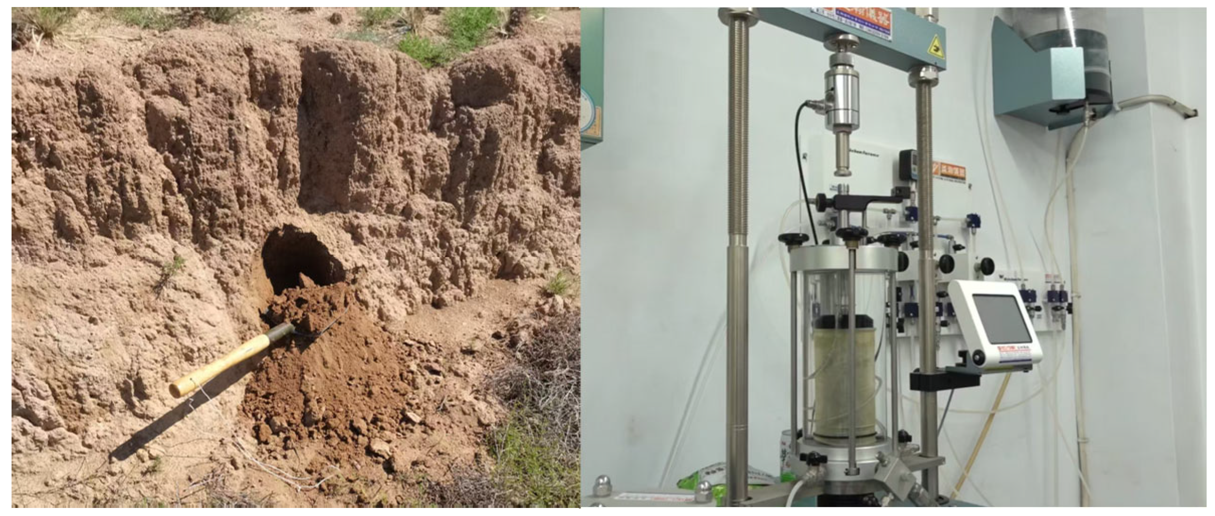
The location of the soil-sampling site (39.9° N, 118.3° E) is shown in Figure 2. Prior to the test, direct-shear measurements under consolidated-undrained (CU) conditions yielded the following average mechanical properties: cohesion c = 18.4 ± 1.2 kPa, internal friction angle φ = 26.7 ± 0.8°, and bulk unit weight γ = 19.5 kN m−3 (3 replicates). The soil profile photograph is shown in Figure 3.
The soil container was fitted with one layer of permeable stones at the bottom to act as filters and prevent soil erosion. Copper electrodes were embedded in the soil at a spacing of 3 cm along the centerline of the container. The electrodes were partially insulated with electrical tape to facilitate adjustment of the signal collection depth. The experimental setup is illustrated in Figure 4.
The SP signals were acquired using a system based on the STM32 microcontroller (STMicroelectronics, Geneva, Switzerland), which controlled a 24-bit analog-to-digital converter (ADC) chip (ADS1256 Texas Instruments, Dallas, TX, USA) to collect signals from nine electrodes. The system included a front-end filter module to reduce high-frequency noise and protect against electrostatic pulses. The average noise level of the acquisition system was approximately 50 μV, which is within the acceptable range for detecting SP signals. The system used fresh copper electrodes to minimize the effects of galvanic cell potentials, and low-mineralization drinking water was used as the seepage supply to reduce redox reactions. Electrodes were zeroed in deionized water; gain/offset coefficients were determined with a 100 mV reference source; and crosstalk was < 1%.
A Python3.6-based data acquisition software was developed to receive and process the SP data in real time. The software displayed the current signal values of all measurement points and saved the data to a CSV file for further analysis.
The soil container was tilted at a 40° angle (as shown in Figure 4) to simulate a sloping surface. Artificial rainfall was applied to the soil surface using a variable-rate spray nozzle. The rainfall intensity was set at 2 mm/h, and the SP signals were recorded over time. Two rows of electrodes were used, with one row buried at a depth of 2 cm and the other at 10 cm, to capture the SP signals at different depths.
The SP data were processed to remove noise and artifacts. The time-domain and spatial-domain characteristics of the SP signals were analyzed to identify patterns associated with seepage, saturation, and structural changes within the soil. The data were also used to develop a dynamic early-warning model based on statistical methods, such as sliding t-tests and Pettitt mutation tests. These methods were employed to detect significant changes in the SP signals that could indicate the onset of landslide instability.

3. Results and Discussion

3.1. Sensitive Recognition Effect on Seepage

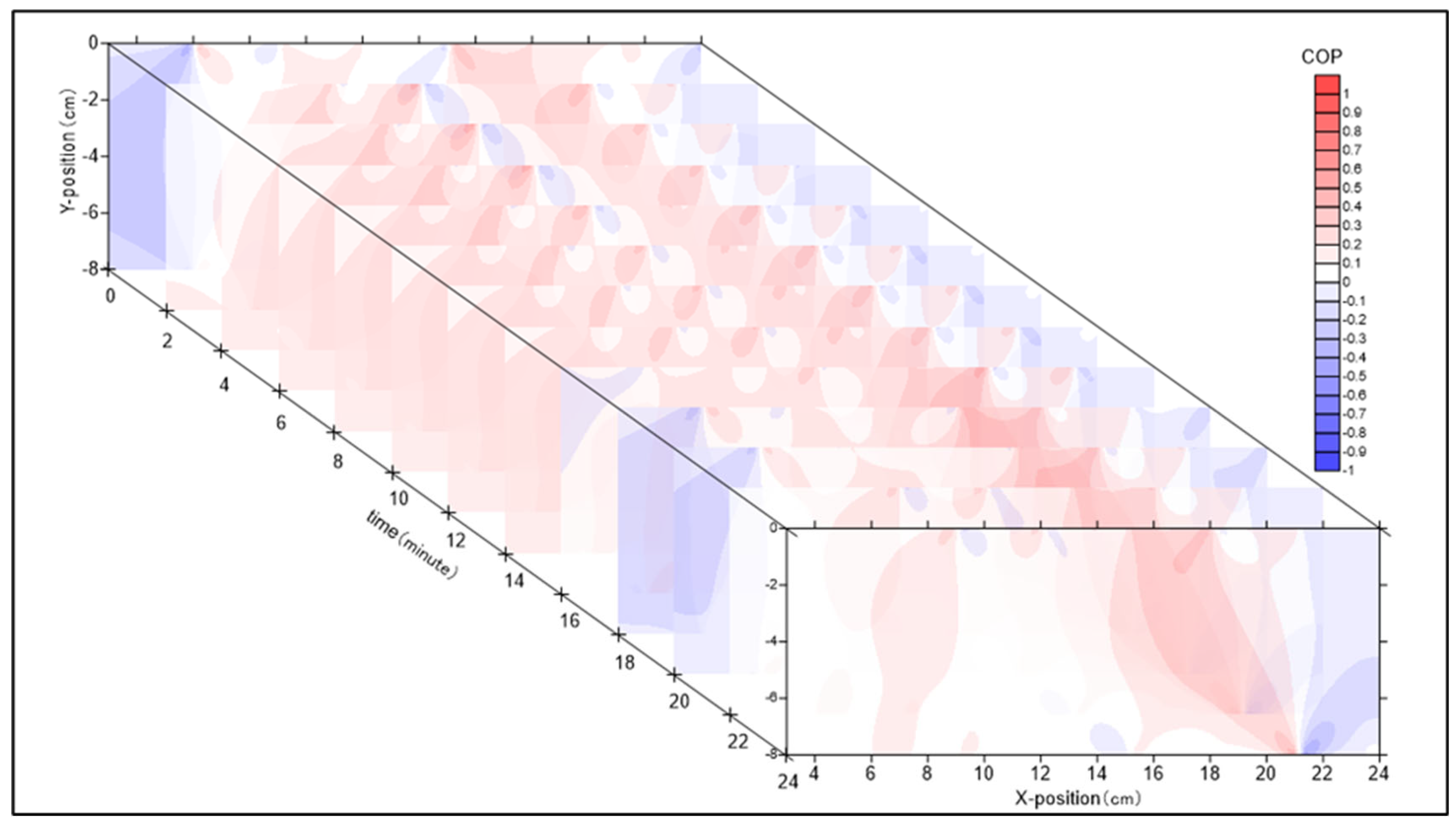
In order to facilitate comparison with the seepage in the profile, we use the COP value calculation method of Patella [29,30,31,32] to inverse the self-potential data into the probability value of charge occurrence.
The slope rainfall simulation experiments revealed rapid and dynamic changes in the SP signals in response to varying rainfall intensities. As rainfall began, the SP signals quickly increased, reflecting the rapid rise in soil moisture content and the initiation of seepage. The signals continued to fluctuate during the rainfall process, capturing the dynamic nature of seepage and saturation changes. The SP signals were particularly sensitive to the onset of surface runoff, which was indicated by a sudden drop in the signal amplitude. This result highlights the potential of SP signals for real-time monitoring of rainfall-induced landslides and early detection of critical changes in soil conditions.
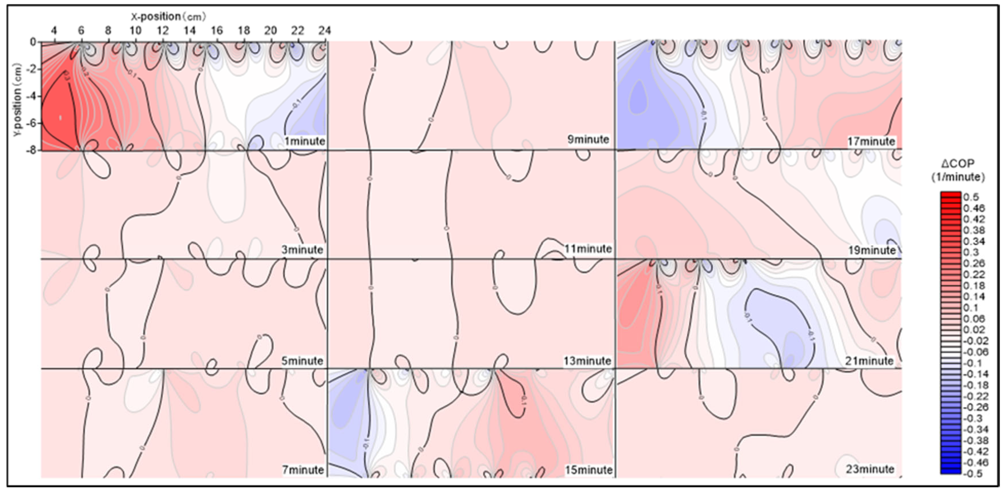
Figure 5 shows the COP tomography profile of SP at each time. It can be observed that the COP is capable of more lucidly reflecting the relationship between the heterogeneous points, as described previously. There is a structural plane between surface electrode 14 (X-position 9 cm) and the bottom electrode 22 (X-position 6 cm), and the charge is accumulated. There is a structural plane between surface electrodes 16 and 17 (X-position 15–18 cm) and the bottom electrode 28 (X-position 21 cm), which accumulates charge. By interpolating the COP at adjacent moments and dividing it by the time interval, the COP growth rate information is recorded as ΔCOP, as shown in Figure 6. ΔCOP has a sensitive recognition effect on the dynamic evolution of seepage flow and creep start-up in slope.
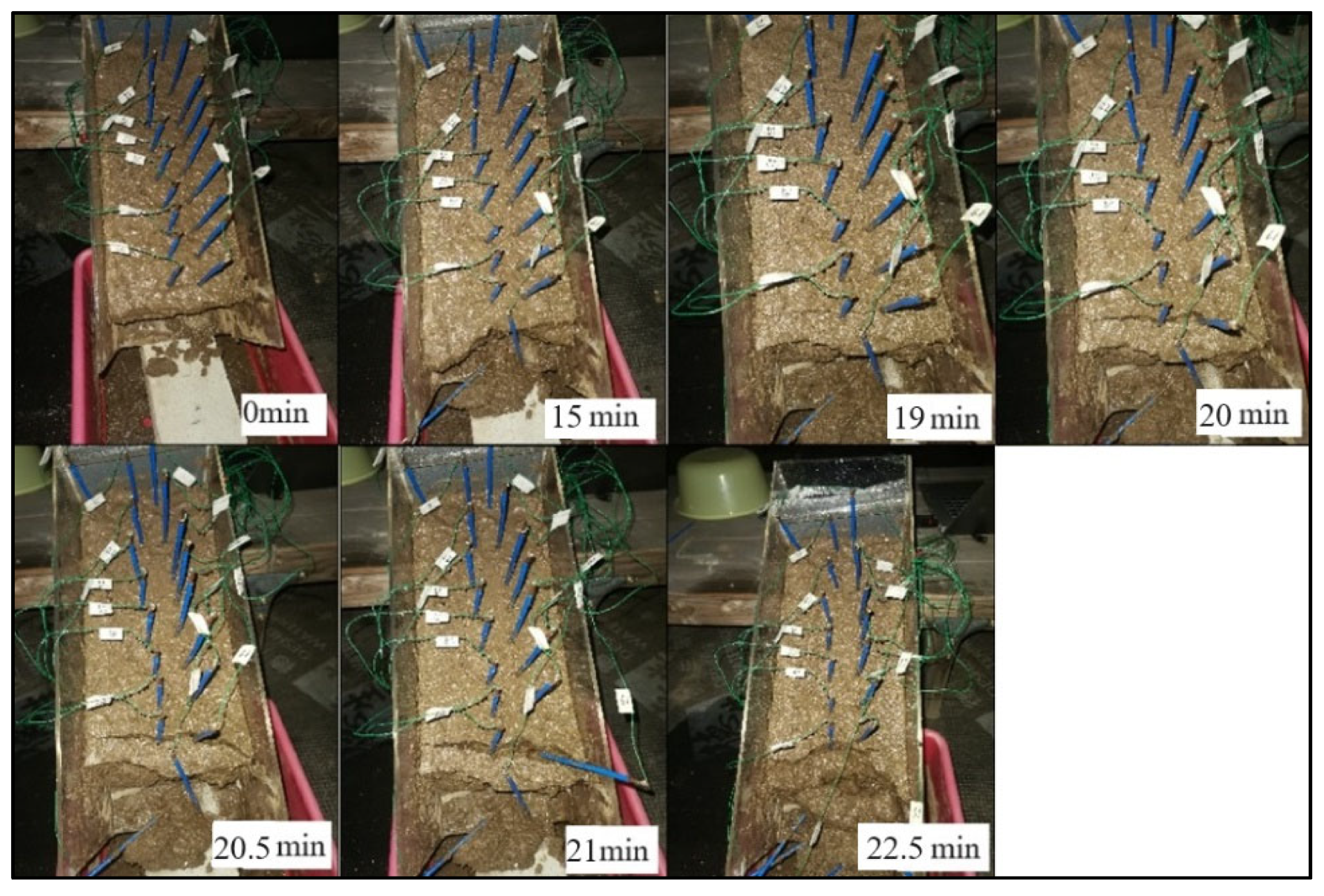
At the beginning, rainfall increases saturation and seepage, and the infiltration rate is fast, which corresponds to the rapid growth in COP at the top of the slope, and then, the COP of the whole slope maintains a slow growth, which corresponds to the decrease in rainfall infiltration rate after surface flow production. At the 15th min, the COP suddenly shows negative growth at the top of the slope, and the growth rate of the middle and lower part of the slope suddenly accelerates, which corresponds to the start of creep. After creep begins, the compressive pore pressure at the lower part of the slope is larger, and the tensile pore pressure at the top of the slope decreases, which corresponds to the negative COP growth at the top of the slope at 15–17 min. The COP growth at the bottom of the slope is accelerated, and the COP in the middle of the slope shows negative growth at 21 min, which corresponds to the greatly weakened seepage flow in the middle of the slope, with the discharge of water in the slope after creep stops, and the pore pressure decreases. The process of slope splitting is shown in Figure 7.

3.2. Dynamic Early-Warning Model

A dynamic early-warning model was developed based on the SP signals to detect early signs of landslide instability. The model utilized statistical methods such as sliding t-tests and Pettitt mutation tests to analyze the SP data and identify significant changes that could indicate the onset of a landslide.
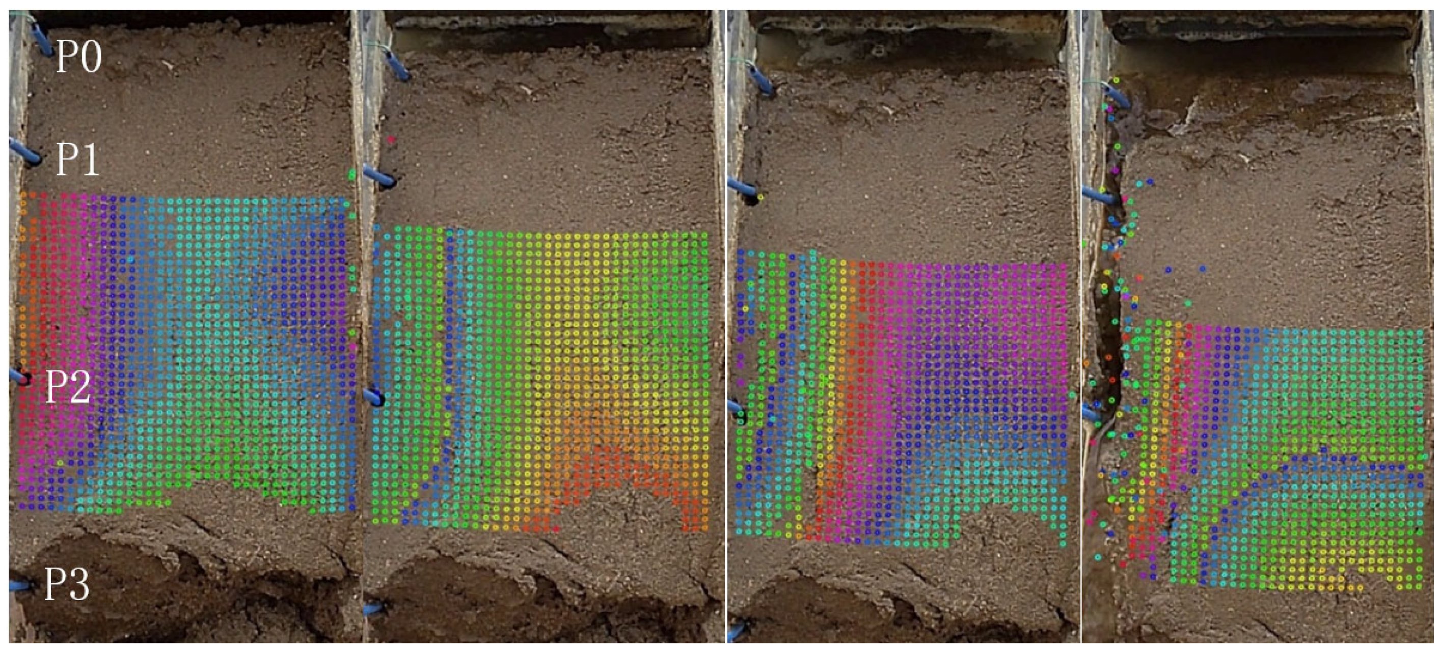
The slope position shift adopted the method of image recognition. To facilitate the shooting of slope surface images, the number of electrodes was reduced to four (P0–P3) with a depth of 2 cm. SP was collected from electrodes P1–P3, with P0 serving as the reference electrode.

3.2.1. Slip-Displacement Measure

In order to study the relationship between slip displacement and SP signal, a timing camera was added on the basis of the above experimental device. By adjusting the camera stand, the camera lens shooting angle was parallel to the slope, and the focus center was at the center of the broken surface. The white balance of the shot was set to automatic, with one frame shot every 3 s. The displacement parameters were obtained using digital image correlation (DIC) technology [30], which draws surface displacement information by comparing the pixel differences of matching features between two frames of images [31,32]. The experiment adopted the PolymerGuy-programmed muDICV2.1.0, which is an open-source software available on Github [33]. The principle of DIC processing is to analyze and compare the regions of interest of the two images before and after and to record the difference between the position with the strongest correlation between each local region in the region of interest and the original position as the displacement of each local point. In this experiment, the analysis area of interest in the image was first set, and then, the average value of all local displacements was taken and saved in the file, so as to record the mean value of the overall displacement of each frame. The initial unit of displacement calculation was pixel (px). In this experiment, the length of the soil tank was 350 mm, and the height of the image pixel was 660 px. Therefore, the conversion ratio was 1 px = 0.53 mm. The displacement of each local point was distinguished by color. The DIC displacement field of the slope in the partial period is shown in Figure 8.
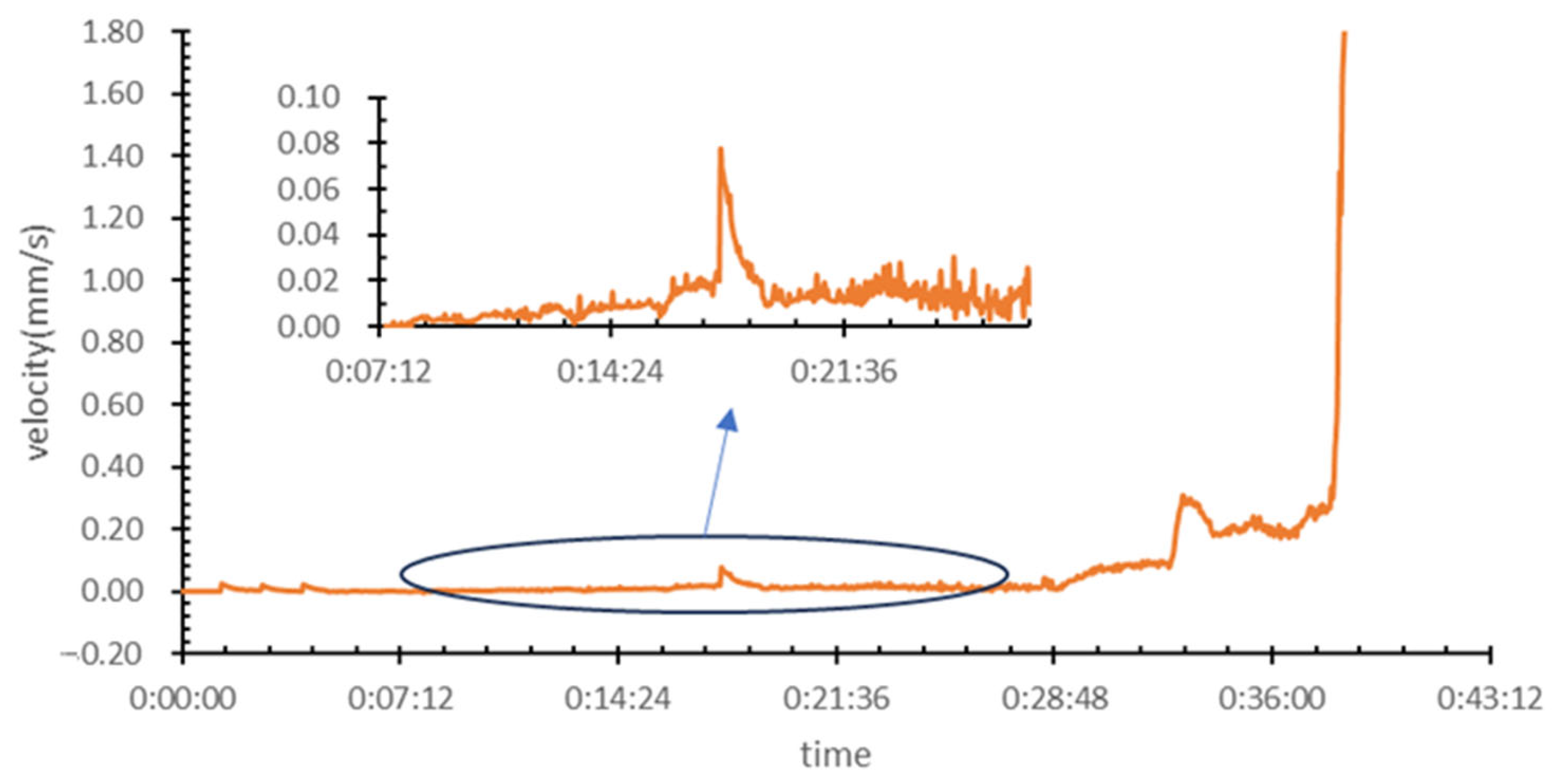
The displacement curve has the characteristics of the Saito model [25] (Figure 9). Figure 10 shows the velocity curve as the derivative of displacement with respect to time. For the first time, the velocity changed dramatically at 18:19, from below 0.01 mm/s to above 0.01 mm/s, which corresponded to the transition from uniform deformation to initial acceleration. A third sudden change in velocity occurred around 29:02, and the velocity continued to increase after the overall increase jump, which corresponded to the transition from the initial acceleration stage to the middle acceleration stage. The velocity changed for the third time at 32:49, from the overall level of 0.06 mm/s to the level of 0.15 mm/s, which corresponded to the transition from the intermediate acceleration stage to the acceleration stage of the slope. The last abrupt change in speed occurred near 38:14, corresponding to the final stage of slope failure.

3.2.2. t-Test and Pettitt Test

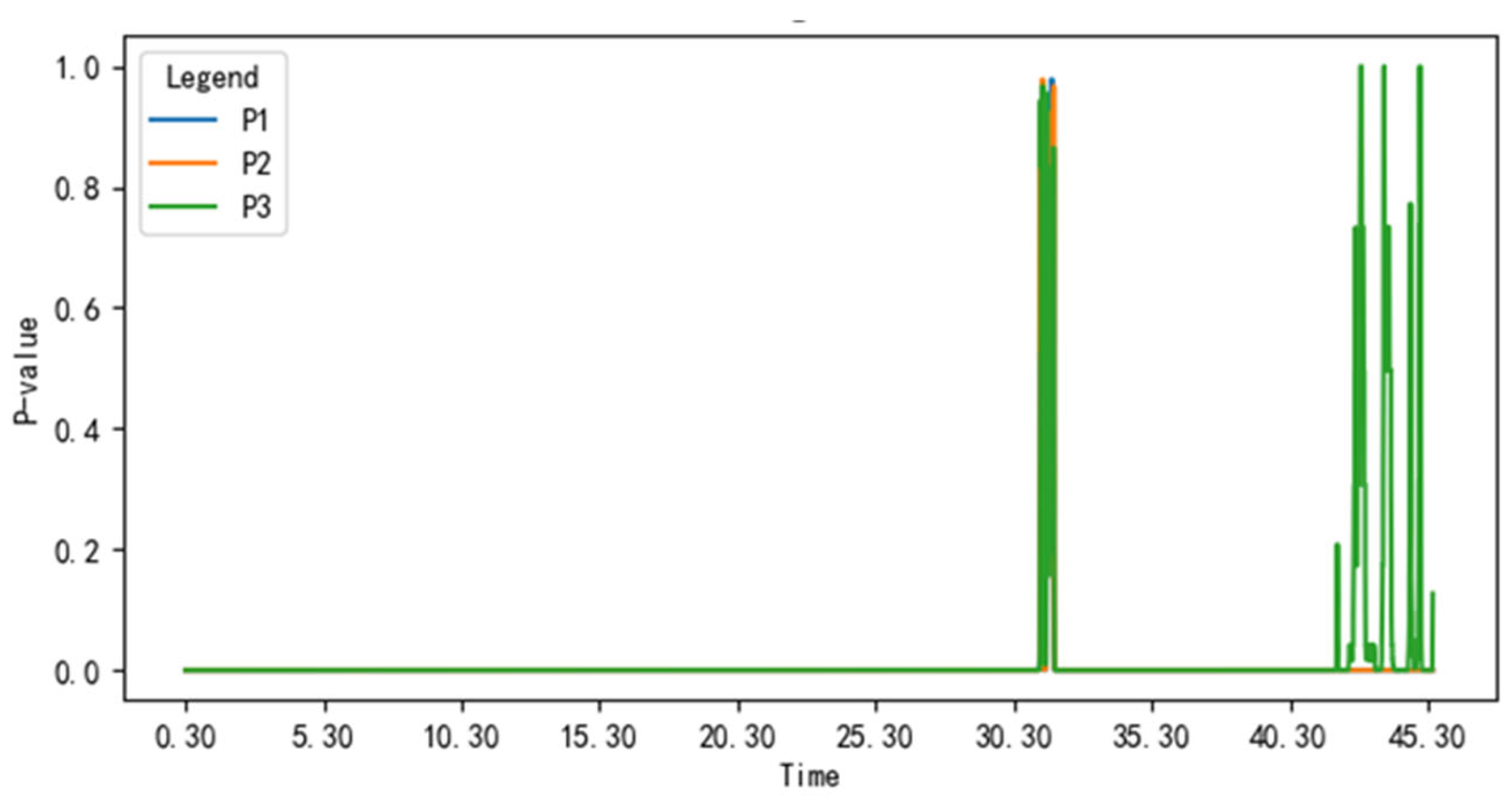
The sliding t-test was applied to the SP data to detect significant changes in the mean value of the signals over time (Figure 11). By comparing the mean values of consecutive signal segments, the sliding t-test identified abrupt changes in the SP signals that could be associated with the initiation of landslide movement. The results showed that the sliding t-test was effective in detecting early-warning signals, with a high sensitivity to changes in the SP data.
From the start time of SP, the data of every 10 time points are a sub-sequence, and the mean and variance of the preceding and following two sub-sequences are expressed as X1, X2, S 1 2 , and S 2 2 , respectively. The formula for calculating the statistic t of the moving t-test is (3). Finally, t is looked up in the table to obtain the mutation probability p value [34].
t = X 1 X 2 S × 1 5
S = 5 ( S 1 2 + S 2 2 ) 9
The abrupt change in SP value mainly occurred in the period of 31.8–32.1 min, indicating that the mean value of SP signal changed significantly during this period, corresponding to the end of the intermediate acceleration stage and the beginning of the acceleration stage.
It was found that finding the change rate (Figure 12) of SP relative to time and then finding the sliding autocorrelation coefficient of this change rate can represent whether the SP changes in the two periods before and after each measurement point table are random, that is, weakly correlated, or whether there is a specific common trend, and the SP changes are consistent, that is, strongly correlated. Then, using the Pettitt mutation test, the corresponding mutation information can be found. The mutation information in this method is represented as the overall level of correlation of SP change becomes larger or smaller.
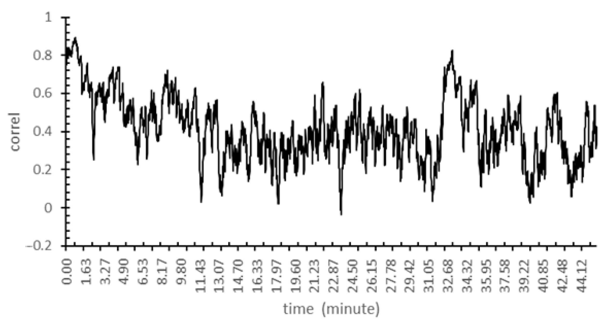
The SP change rate of all observation points was set up with a certain time window as a sub-sequence, and the translation window was taken as a correlation coefficient to obtain the sliding correlation coefficient of the SP change rate (Figure 13).
The Pettitt test is a non-parametric test method [15]. It is used for the correlation coefficient sequence Xi with number n: (i = 1, 2, …, n). The corresponding order is listed as ri: (i = 1, 2, …, n). The constitutive statistic is
S k = 2 i = 1 k r i k n + 1 , k = 1,2 , , n
Sk is the test result. If a mutation occurs at a certain time point, SE = max|Sk|; E is the mutation point; and the p statistic is calculated:
P = 2 e 6 S E 2 n 3 + n 2
If P ≤ 0.05, the mutation point was considered statistically significant. The Pettitt test was carried out on the correlation coefficient. As shown in Figure 14, the mutation point was 33.1 min, and the corresponding p value was 1.99, which was evaluated as insignificant change. It can be considered that the significance of this mutation lies more in identifying the transformation of SP from random change to consistent change, and the randomness of SP change is related to the moisture content and heterogeneity of soil mass. When the water content is low and the heterogeneity is high, the randomness of SP change will increase; otherwise, the consistency of SP change will increase, and the soil water content at this time will be basically stable. The source of randomness is mainly the influence of the instantaneous soil structure change on the heterogeneity; therefore, the mutation significance is not high.
Therefore, the SP sliding t-test is more sensitive to sudden change in displacement, and the SP change rate test is more suitable for studying the random characteristics of soil SP change.

3.2.3. Mahalanobis Distance Test

The Mahalanobis distance [35] is a method for measuring the distance between two points in a multi-dimensional space, which takes into account the covariance structure of the data. For a dataset, its covariance matrix is ∑. The Mahalanobis distance can be used to measure the distance between a point and the center of the dataset (usually the mean) or the distance between two points.
If the outlier phenomenon of SP is regarded as an anomaly, and the SP values of all electrodes at a certain moment are regarded as an SP state vector (Vt) of this state, then the distance between Vt and the mean (Vu) of previous periods is defined as the anomaly degree of this state. Considering that the distribution of SP values among the electrodes is not completely linearly independent and affects the consistency of the geometric distance, the Mahalanobis distance is introduced to eliminate the correlation influence among the electrodes.
D = V t V u T 1 ( V t V u )
V t V u T is the transpose of ( V t V u ) , and 1 is the inverse matrix of the covariance moment   . The obtained D value at this time has scale invariance because it takes into account the covariance structure of the SP data and eliminates the correlation interference, including scale influence [36]. This makes the Mahalanobis distance more effective than other distance measurement methods, such as the Euclidean distance, when dealing with correlated multivariate data.
It is known that the Mahalanobis distance in Figure 15 is derived from the SP data of the three electrodes and conforms to the χ2 distribution with three degrees of freedom. By looking up the χ2 distribution, it can be found that the cumulative probability of D = 3 is 97.1%, and the cumulative probability of 5 is 99.9%. Therefore, the state with a Mahalanobis distance of 5 can represent a 99.9% probability of a sudden mutation anomaly. A comparison with Figure 8 reveals that the abnormal moments all correspond to abnormal acceleration situations. Even the slight acceleration in the initial period from 1:16 to 2:32 is strengthened and magnified in the Mahalanobis distance of SP.

3.3. Implications for Landslide Monitoring and Early Warning

The summary of the numerical results is as follows: (i) The maximum SP amplitude is 30 mV at rainfall onset, changing from 56 to 14 mV at failure. (ii) The horizontal displacement is 150 mm at failure, indicated by the black line and data label in Figure 9. (iii) The statistical thresholds are as follows: Mahalanobis distance κ = 5.0 ± 0.1 (Figure 15), sliding t-test p > 0.9 (Figure 11), and Pettitt breakpoint t = 1980 s, annotated with green dashed lines and corresponding labels in Figure 14.
The findings of this study have important implications for the application of SP signals in landslide monitoring and early-warning systems. Compared with the existing landslide monitoring technologies (Table 2), the advantages of this study include the high sensitivity of SP signals to seepage, saturation, and soil heterogeneity, making them a valuable tool for real-time monitoring of landslide conditions. The developed dynamic early-warning model based on SP signals demonstrated the potential for early detection of landslide instability, providing valuable time for the implementation of mitigation measures.
Future research should focus on optimizing the SP monitoring system and enhancing its applicability under various geological conditions. This includes the development of more advanced statistical models and the integration of SP signals with other monitoring techniques to create comprehensive landslide monitoring systems. Additionally, further studies should explore the long-term stability of SP signals and their response to different environmental factors, such as temperature and soil composition.

3.4. Field-Scale Prospects

3.4.1. Electrode Layout and Spacing

The 3 × 3 planar grid used in the 0.35 m wide flume can be scaled linearly. Assuming a typical landslide width of 30–50 m, the same nine electrodes would be deployed at 5–8 m spacing along the slope axis, yielding a longitudinal resolution comparable to that achieved in the laboratory (≈ 0.1 L, where L is slope length). Multi-channel acquisition units (24-bit, 32-node) now commercially available allow >100 electrodes to be read at 1 Hz with <1 W power consumption.

3.4.2. Electrode Type and Installation Depth

Non-polarizing Cu–CuSO4 electrodes (Ø 20 mm, 150 mm long) can be driven by hand-held percussion tools to depths of 0.5–2 m, corresponding to the upper shear-band zone observed in most shallow landslides. Contact resistance remains below 1 kΩ in clayey–sandy soils, ensuring the same signal-to-noise ratio as in the flume.

3.4.3. Limitations and Next Steps

Lateral heterogeneity, vegetation, and anthropogenic noise may reduce signal quality; these effects will be quantified in an upcoming field campaign. Until those data are available, the present results should be regarded as a proof of concept rather than a turnkey solution.
In studying the application of self-potential (SP) monitoring technology in landslide early warning, its high sensitivity to slope seepage, saturation, and structural changes can be mutually corroborated with several related studies. The joint particle size calculation model (JCM) proposed by Jichao Sun [42] realizes efficient simulation of rock and soil particles through a neural network method, revealing the inherent connection between particle gradation and mechanical properties, which provides a reference for understanding the influence of internal particle movement in landslide bodies on SP signals at the micro-mechanical level. The monitoring study on ground deformation in Beijing found that precipitation and surface soil moisture have a positive correlation with land subsidence [43], which is consistent with the law of dynamic changes in SP signals with rainfall intensity in the rainfall simulation experiments of this study, indicating the universality of the impact of hydrological factors on the electrical properties of geological bodies. The study on ecological water demand in the Yongding River Basin shows that changes in water resources can significantly affect ecosystem stability [44], suggesting that in landslide early warning, it is necessary to analyze abnormal changes in SP signals in combination with regional hydrological backgrounds. The migration of ground sediment [45] can lead to engineering problems such as reduced stability of riverbanks, and the mutation of SP signals when slope cracks occur in this study may be an electrical response caused by internal sediment migration. The study on the periodic characteristics of extreme rainfall in Shenzhen [46] provides a reference for understanding the temporal patterns of rainfall-induced landslides, which is helpful for optimizing the time scale setting of SP monitoring. The study on the spatiotemporal characteristics of precipitation in Harbin [47] further indicates that changes in long-term precipitation patterns may affect the reference value of SP signals by altering the moisture state of rock and soil bodies, which is of great significance for establishing regional SP monitoring baselines. These studies corroborate the feasibility and complexity of SP monitoring in geological disaster early warning from different perspectives, providing a multi-disciplinary basis for improving early warning models.

4. Conclusions

This study advances landslide early-warning practice through two tightly integrated contributions. Over a series of controlled flume experiments that imposed progressive rainfall and cracking sequences on a simulation slope, we first documented how self-potential (SP) signals evolve in lockstep with seepage fronts, saturation changes, and incipient shear. These observations confirmed that minute electrokinetic fluctuations precede visible deformation by a measurable interval, validating SP as a real-time proxy for internal destabilization. Building on this evidence, we found some anomaly prediction parameters based on SP, such as the Mahalanobis distance.
For construction industry application, we created a workflow that converts raw voltage traces into early-warning flags without recourse to tracers or additional sensors. Finally, the entire sensing chain—thin electrodes, an STM32 acquisition board, and open-source wireless protocols—was packaged into a lightweight, plug-and-play kit that can be installed on cut slopes, embankments, or tunnel portals by routine site personnel. The resulting system therefore offers the construction industry a low-cost, easily scalable complement to traditional inclinometer or piezometer arrays, enabling proactive slope-safety management from initial excavation through long-term operation.

Author Contributions

Conceptualization, C.Y.; Methodology, C.Y.; Software, C.Y.; Formal analysis, C.Y.; Writing—original draft, C.Y.; Writing—review & editing, J.S.; Supervision, J.S. All authors have read and agreed to the published version of the manuscript.

Funding

This research received no external funding.

Institutional Review Board Statement

Not applicable.

Informed Consent Statement

Not applicable.

Data Availability Statement

The data supporting the findings of this study are available from the corresponding author upon reasonable request. Please contact the corresponding author at sunjc@cugb.edu.cn.

Acknowledgments

We are grateful to the reviewers and editors for their constructive feedback, which helped improve the quality of this manuscript. Their expertise and dedication are highly appreciated.

Conflicts of Interest

The authors declare that there are no conflicts of interest regarding the publication of this article. The research was conducted independently, and the authors have no financial or personal relationships with any individuals or organizations that could have inappropriately influenced the work presented in this paper.

Abbreviations

The following abbreviations are used in this manuscript:
SPSelf-Potential
COPCharge Occurrence Probability
DICDigital Image Correlation

References

  1. Hungr, O.; Leroueil, S.; Picarelli, L. The Varnes classification of landslide types, an update. Landslides 2014, 11, 167–194. [Google Scholar] [CrossRef]
  2. United Nations Office for Disaster Risk Reduction (UNDRR). Global Assessment Report on Disaster Risk Reduction; UNDRR: Geneva, Switzerland, 2024. [Google Scholar]
  3. IPCC. Climate Change 2021: The Physical Science Basis. Contribution of Working Group I to the Sixth Assessment Report of the Intergovernmental Panel on Climate Change; IPCC: Geneva, Switzerland, 2021. [Google Scholar]
  4. Zhang, M.; Yin, Y.; Huang, B. Mechanism and emergency mitigation of Shenzhen landslide on December 20, 2015. Landslides 2016, 13, 215–229. [Google Scholar]
  5. United Nations Office for Disaster Risk Reduction. Colombia—Mocoa Debris Flow 2017: UNDRR Situation Report; UNDRR: Geneva, Switzerland, 2017. [Google Scholar]
  6. Walter, T.R.; Haghighi, M.H.; Schneider, F.M.; Coppola, D.; Motagh, M.; Saul, J.; Babeyko, A.; Dahm, T.; Troll, V.R.; Tilmann, F.; et al. Complex hazard cascade culminating in the Anak Krakatau sector collapse. Nat. Commun. 2019, 10, 4339. [Google Scholar] [CrossRef]
  7. Mishra, P.K.; Rawat, K.S.; Rawat, G. Rainfall-induced landslides in Pettimudi, Western Ghats, India: Causes and consequences. Landslides 2021, 18, 713–728. [Google Scholar]
  8. Japan Meteorological Agency. Report on Heavy Rain Disasters Associated with Typhoon Nanmadol in September 2022; JMA: Tokyo, Japan, 2022. [Google Scholar]
  9. Uhlemann, S.; Maurer, H.; Zimmermann, G. Landslide investigation and monitoring using self-potential methods. Near Surf. Geosci. Conf. Exhib. 2019, 167, 138–150. [Google Scholar]
  10. Hattori, K.; Yabe, S.; Otsubo, H. Self-Potential Approach to Early Warning for Rainfall-induced Landslide. In AGU Fall Meeting Abstracts; AGU Publication: Washington, DC, USA, 2011; Volume 2011, p. NH13F-1435. [Google Scholar]
  11. Yabe, S.; Hattori, K.; Otsubo, H. In-situ self potential and soil moisture measurement for rainfall induced landslide at Pelabuhan Ratu, Indonesia. In AGU Fall Meeting Abstracts; AGU Publication: Washington, DC, USA, 2011; Volume 2011, p. NH13F-1441. [Google Scholar]
  12. Yamazaki, T.; Hattori, K.; Kaneda, H.; Sakai, H.; Izumi, Y.; Terajima, T. Development of Monitoring System to Understand Preparation Processes of Rainfall-Induced Landslides Estimation of Slip Surface and In Situ Observation Using Electromagnetic Methods. Electron. Commun. Jpn. 2017, 100, 3–11. [Google Scholar] [CrossRef]
  13. Hu, K.; Mo, C.; Zhang, Y.; Li, S.; Sun, J.; Han, P.; Huang, Q. An experimental study on monitoring an indoor landslide based on self-potential method. Chin. J. Geophys. 2021, 64, 4582–4593. (In Chinese) [Google Scholar] [CrossRef]
  14. Beamish, D.; Peart, M.R. Electrokinetic geophysics—A review. Terra Nova 1998, 10, 48–55. [Google Scholar] [CrossRef]
  15. Revil, A.; Schwaeger, H.; Cathles, L.M., III; Manhardt, P.D. Streaming potential in porous media 2. Theory and application to geothermal system. J. Geophys. Res. 1999, 104, 20033–20048. [Google Scholar] [CrossRef]
  16. Revil, A.; Finizola, A.; Gresse, M. Self-potential as a tool to assess groundwater flow in hydrothermal systems: A review. J. Volcanol. Geotherm. Res. 2023, 437, 107788. [Google Scholar] [CrossRef]
  17. Ishido, T.; Mizutani, H. Experimental and theoretical basis of electrokinetic phenomena in rock-water systems. J. Geophys. Res. 1981, 86, 1763–1775. [Google Scholar] [CrossRef]
  18. Jouniaux, L.; Ishido, T. Electrokinetics in Earth sciences: A tutorial. Int. J. Geophys. 2012, 2012, 286107. [Google Scholar] [CrossRef]
  19. Bolèkve, J.; Revil, A.; Janod, F.; Mattiuzzo, J.; Fry, J. Preferential fluid flow pathways in embankment dams imaged by self-potential tomography. Near Surf. Geophys. 2009, 7, 447–462. [Google Scholar] [CrossRef]
  20. Darnet, M.; Marquis, G. Modelling streaming potential (SP) signals induced by water movement in the vadose zone. J. Hydrol. 2004, 285, 48–61. [Google Scholar] [CrossRef]
  21. Guichet, X.; Jouniaux, L.; Pozzi, J.P. Streaming potential of a sand column in partial saturation conditions. J. Geophys. Res. 2003, 108, 2141. [Google Scholar] [CrossRef]
  22. Boleve, A.; Vandemeulebrouck, J.; Grangeon, J. Laboratory validation of streaming-potential monitoring for rainfall-induced landslides. Landslides 2021, 18, 215–229. [Google Scholar]
  23. Trique, M.; Garambois, S.; Sailhac, P. Field-scale evidence of streaming potential response to slope failure in clayey embankments. Eng. Geol. 2022, 304, 106693. [Google Scholar]
  24. Sheffer, M.R.; Oldenburg, C.M.; Grant, S.L.; Harris, R.N.; Levy, Z.F.; Revil, A. Self-potential monitoring of rainfall-induced landslides: Field-scale validation. Eng. Geol. 2021, 290, 106212. [Google Scholar]
  25. Saito, M. Forecasting time of slope failure by tertiary creep. In Proceedings of the 7th International Conference on Soil Mechanics and Foundation Engineering, Held in Mexico City, 1969; Mexican Society of Mechanics: Mexico City, Mexico, 1969; Volume 2, pp. 677–683. [Google Scholar]
  26. Vichabian, Y.; Morgan, F.D. Self-potential mapping of seepage in embankment dams. J. Environ. Eng. Geophys. 2002, 7, 59–68. [Google Scholar]
  27. Rizzo, E.; Suski, B.; Revil, A.; Straface, S.; Troisi, S. Self-potential signals associated with pumping tests experiments. J. Hydrol. 2004, 285, 48–61. [Google Scholar] [CrossRef]
  28. Uhlemann, S.; Smith, A.; Chambers, J.; Dixon, N.; Dijkstra, T.; Haslam, E.; Mackay, J. Assessment of ground-based monitoring techniques applied to landslide investigations. Geomorphology 2016, 253, 438–451. [Google Scholar] [CrossRef]
  29. Patella, D. Introduction to ground surface self-potential tomography. Geophys. Prospect. 1997, 45, 653–681. [Google Scholar] [CrossRef]
  30. Heid, B.; Kääb, A. Evaluation of existing image matching algorithms for deriving glacier surface displacements from optical satellite imagery. Remote Sens. Environ. 2012, 124, 339–355. [Google Scholar] [CrossRef]
  31. Li, J.; Zhang, Z. Digital image correlation for landslide monitoring: A review and case study. Geomat. Nat. Hazards Risk 2021, 12, 1–20. [Google Scholar]
  32. Bickel, S.; Strozzi, T.; Farinotti, D. Systematic quantification and assessment of digital image correlation for landslide displacement monitoring. Remote Sens. Environ. 2023, 15, 6223. [Google Scholar]
  33. Solav, D.; Moerman, K.M.; Jaeger, A.M.; Genovese, K.; Herr, H.M. MultiDIC: An open-source toolbox for multi-view 3D digital image correlation. IEEE Access 2018, 6, 30520–30535. [Google Scholar] [CrossRef]
  34. Pettitt, A.N. A non-parametric approach to the change-point problem. J. R. Stat. Soc. Ser. C Appl. Stat. 1979, 28, 126–135. [Google Scholar] [CrossRef]
  35. Mahalanobis, P.C. On the generalized distance in statistics. Proc. Natl. Inst. Sci. India 1936, 2, 49–55. [Google Scholar]
  36. Galeano, P.; Gómez-Valencia, A.; Lopez, P. The Mahalanobis distance for functional data with applications to classification. J. Appl. Stat. 2015, 42, 2268–2283. [Google Scholar] [CrossRef]
  37. Monserrat, O.; Crosetto, M.; Luzi, G. A review of ground-based SAR interferometry for deformation measurement. ISPRS J. Photogramm. Remote Sens. 2014, 93, 40–48. [Google Scholar] [CrossRef]
  38. Wang, J.; Gao, J.; Liu, C.; Wang, J. High precision slope deformation monitoring model based on the GPS/Pseudolites technology in open-pit mine. Min. Sci. Technol. 2010, 20, 126–132. [Google Scholar] [CrossRef]
  39. Yadav, D.K.; Karthik, G.; Jayanthu, S.; Das, S.K. Design of real-time slope monitoring system using time-domain reflectometry with wireless sensor network. IEEE Sens. Lett. 2019, 3, 2500304. [Google Scholar] [CrossRef]
  40. Yang, B.; Aminossadati, S.M.; Chen, Z.; Kizil, M.S. Fibre optic sensing based slope crest tension crack monitoring system for surface mines. In Proceedings of the 2nd International Conference for Fibre-Optic and Photonic Sensors for Industrial and Safety Applications (OFSIS), Brisbane, QLD, Australia, 8–10 January 2017; pp. 27–32. [Google Scholar]
  41. Bar, N.; Kostadinovski, M.; Tucker, M.; Byng, G.; Rachmatullah, R.; Maldonado, A.; Pötsch, M.; Gaich, A.; McQuillan, A.; Yacoub, T. Rapid and robust slope failure appraisal using aerial photogrammetry and 3D slope stability models. Int. J. Min. Sci. Technol. 2020, 30, 651–658. [Google Scholar] [CrossRef]
  42. Sun, J. Joint particle size calculation model (JCM): A neural network approach for efficient rock and soil simulation. Baltica 2025, 38, 32–44. [Google Scholar] [CrossRef]
  43. Zheng, Y.; Sun, J. Monitoring Ground Deformation in Beijing and Analysis of Influencing Factors. Int. J. Ground Sediment Water 2025, 21, 1557–1578. [Google Scholar]
  44. Fu, Y.; Sun, J. Water Ecological Demands and Supplementary Water Supply in the Yongding River Basin, China. Int. J. Ground Sediment Water 2025, 22, 1759–1770. [Google Scholar]
  45. Sun, J. Survey and research frame for ground sediment. Environ. Sci. Pollut. Res. 2016, 23, 18960–18965. [Google Scholar] [CrossRef]
  46. Wang, X.; Sun, J. The Temporal Evolution Characteristics of Extreme Rainfall in Shenzhen City, China. Sustainability 2025, 17, 3512. [Google Scholar] [CrossRef]
  47. Fu, Y.; Sun, J. Spatiotemporal characteristics of precipitation in Harbin City, China, from 1962 to 2020. Front. Environ. Sci. 2025, 13, 1550421. [Google Scholar] [CrossRef]
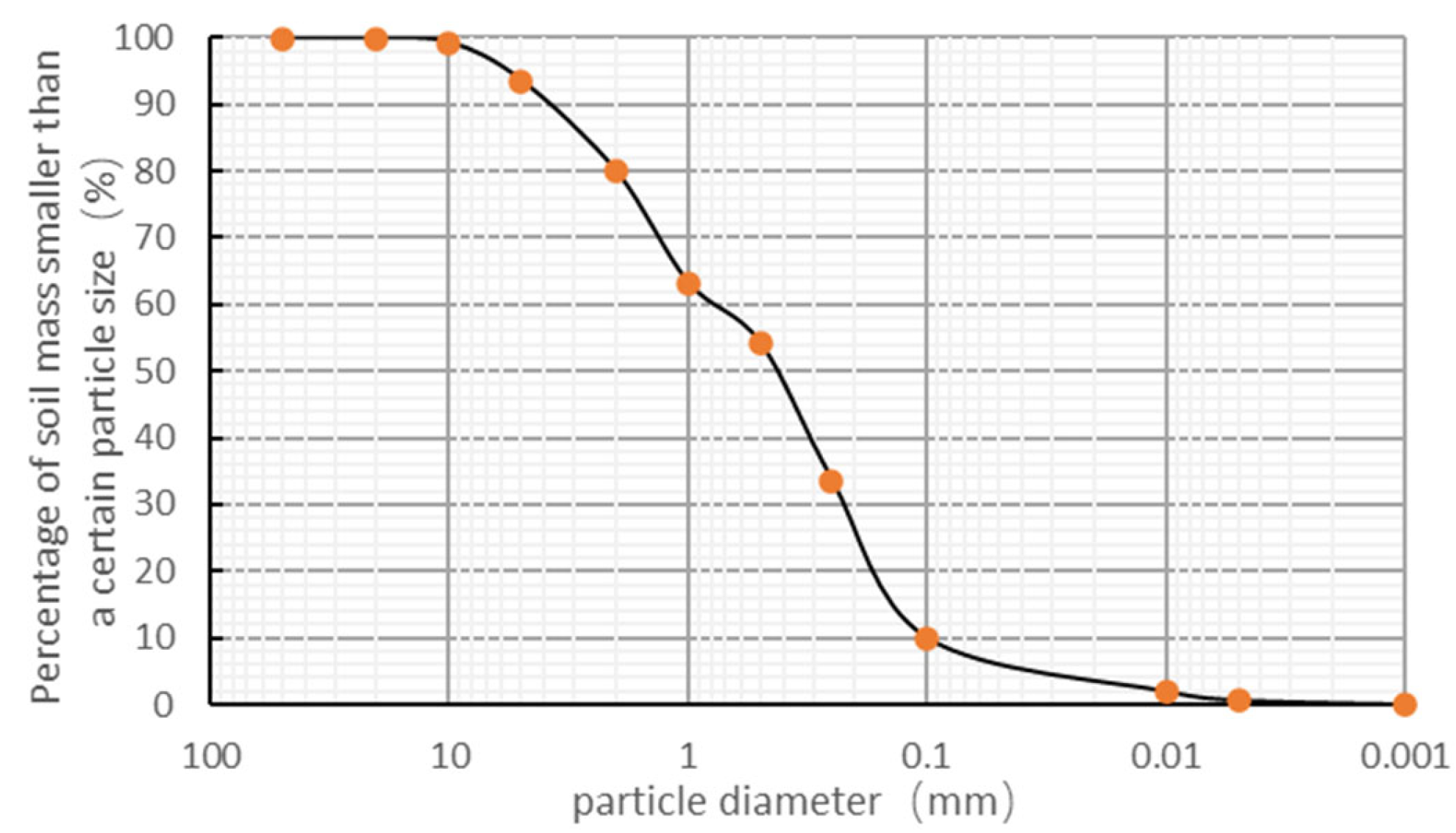
Figure 1. Particle size distribution of the experimental soil.
Applsci 15 09037 g001
Figure 2. Geographic map of the soil-sampling site (red star).
Applsci 15 09037 g002
Figure 3. Soil profile photograph (left—collected soil, right—remolded test).
Applsci 15 09037 g003
Figure 4. Slope rainfall simulation setup.
Applsci 15 09037 g004
Figure 5. Time series of COP chromatographic profile (transparency 70%).
Applsci 15 09037 g005
Figure 6. Time series of ΔCOP profile.
Applsci 15 09037 g006
Figure 7. The process of slope cracking.
Applsci 15 09037 g007
Figure 8. DIC displacement field of the slope in the partial period (the color cycles indicate relative displacement; one full spectrum (red → violet) corresponds to about 12 mm horizontal movement).
Applsci 15 09037 g008
Figure 9. Average displacement and SP synchronous observation data.
Applsci 15 09037 g009
Figure 10. Average moving velocity curve of slope surface.
Applsci 15 09037 g010
Figure 11. SP sliding t-test.
Applsci 15 09037 g011
Figure 12. SP change rate.
Applsci 15 09037 g012
Figure 13. Sliding correlation coefficient of SP change rate.
Applsci 15 09037 g013
Figure 14. SP change rate mutation (Pettitt mutation test) Red line: Mean value before and after mutation, Green line: Position where the significance of the mutation is P < 0.05.
Applsci 15 09037 g014
Figure 15. The Mahalanobis distance curves of the SP state at various times (yellow line D = 5).
Applsci 15 09037 g015
Table 1. Representative landslide events and their primary triggers in recent years.
No.Event (Year)Country/RegionPrimary TriggerReference
1Shenzhen “12·20” landslide (2015)ChinaOverloading of artificial fill + rainfall infiltration[4]
2Mocoa debris flow (2017)ColombiaExtreme rainfall + loose volcanic deposits[5]
3Anak Krakatau flank collapse (2018)IndonesiaVolcanic activity + wave erosion[6]
4Pettimudi landslide (2020)IndiaIntense rainfall + thin residual soil layer[7]
5Honshu landslides (2022)JapanTyphoon Nanmadol extreme rainfall[8]
Table 2. Comparison of representative slope-monitoring techniques, installations, and underlying theories.
CategoryRepresentative Device/MethodPrimary Theoretical BasisAdvantagesLimitationsComparison with This Study
Surface displacementGPS, total station, InSAR [37,38]Triangulation/interferometric phaseHigh accuracy (mm), wide coverageExpensive, weather-sensitive, delayed response to internal failureLow-cost and directly senses internal seepage
Sub-surface displacementInclinometer, TDR cable [39]Tilt/time-domain reflectometryMeasures depth to sliding surfaceRequires drilling, sparse point dataElectrode array avoids drilling
Pore-water pressureVibrating-wire/fiber-optic piezometers [40]Terzaghi effective-stress principleDirect pressure reading, well-establishedPoint measurement only, no spatial saturation mapSP reflects spatial seepage field
Geophysical imagingERT, seismic tomography [41]Resistivity/velocity tomography3D imaging, rich informationHeavy equipment, complex processing, low real-time capabilityLightweight and delivers real-time data
Acoustic emission/micro-seismicAE sensorsKaiser effect, micro-crack detectionSensitive to micro-crackingHigh background noise, dense sensor network requiredSP shows higher SNR with fewer sensors
Traditional SPPeriodic manual surveysHelmholtz–Smoluchowski equationContinuous, non-intrusiveOffline, lacks automated warning modelIntegrates continuous SP with Mahalanobis–COP real-time alerts
Disclaimer/Publisher’s Note: The statements, opinions and data contained in all publications are solely those of the individual author(s) and contributor(s) and not of MDPI and/or the editor(s). MDPI and/or the editor(s) disclaim responsibility for any injury to people or property resulting from any ideas, methods, instructions or products referred to in the content.