Article

From Convolution to Spikes for Mental Health: A CNN-to-SNN Approach Using the DAIC-WOZ Dataset

by
Victor Triohin
1,
Monica Leba
2,* and
Andreea Cristina Ionica
3
1
Doctoral School, University of Petroșani, 332006 Petrosani, Romania
2
System Control and Computer Engineering Department, University of Petroșani, 332006 Petrosani, Romania
3
Management and Industrial Engineering Department, University of Petroșani, 332006 Petrosani, Romania
*
Author to whom correspondence should be addressed.
Appl. Sci. 2025, 15(16), 9032; https://doi.org/10.3390/app15169032
Submission received: 28 July 2025 / Revised: 7 August 2025 / Accepted: 14 August 2025 / Published: 15 August 2025
(This article belongs to the Special Issue eHealth Innovative Approaches and Applications: 2nd Edition)

Abstract

Featured Application

This work enables energy-efficient, real-time depression screening from speech, with potential applications in mobile health platforms, telemedicine, and low-resource clinical settings.

Abstract

Depression remains a leading cause of global disability, yet scalable and objective diagnostic tools are still lacking. Speech has emerged as a promising non-invasive modality for automated depression detection, due to its strong correlation with emotional state and ease of acquisition. While convolutional neural networks (CNNs) have achieved state-of-the-art performance in this domain, their high computational demands limit deployment in low-resource or real-time settings. Spiking neural networks (SNNs), by contrast, offer energy-efficient, event-driven computation inspired by biological neurons, but they are difficult to train directly and often exhibit degraded performance on complex tasks. This study investigates whether CNNs trained on audio data from the clinically annotated DAIC-WOZ dataset can be effectively converted into SNNs while preserving diagnostic accuracy. We evaluate multiple conversion thresholds using the SpikingJelly framework and find that the 99.9% mode yields an SNN that matches the original CNN in both accuracy (82.5%) and macro F1 score (0.8254). Lower threshold settings offer increased sensitivity to depressive speech at the cost of overall accuracy, while naïve conversion strategies result in significant performance loss. These findings support the feasibility of CNN-to-SNN conversion for real-world mental health applications and underscore the importance of precise calibration in achieving clinically meaningful results.

1. Introduction

Depression, or major depressive disorder, is one of the most pressing global health concerns of the 21st century. With over 350 million people affected worldwide and lifetime prevalence rates reaching up to 15%, depression is the leading cause of disability globally, accounting for more than 7.5% of all years lived with disability (YLD) [1,2,3]. Recent epidemiological data underscore the growing burden of depression across all age groups, particularly among adolescents and young adults. In the United States, prevalence rates have surpassed 19% among adolescents [4,5], while in Europe and Asia, point prevalence ranges from 5–10% and up to 16.7%, respectively, with significantly higher disability-adjusted life years (DALYs) in younger populations [6,7,8]. The COVID-19 pandemic further exacerbated this trend, with global symptoms of depression spiking above 20% in many adult cohorts and nearly 30% in some regions [9,10]. These figures highlight a deepening crisis that transcends cultural and economic boundaries, emphasizing the urgent need for scalable, accurate, and accessible diagnostic solutions.
Current diagnostic practices for depression, which rely heavily on structured interviews and self-report questionnaires such as the Patient Health Questionnaire PHQ-8 and PHQ-9, face critical limitations including subjectivity, underreporting, and limited scalability—particularly in low-resource or stigmatized environments [11,12,13]. In this context, machine learning (ML) offers a promising avenue for non-invasive, objective depression detection. Among various modalities, speech has emerged as an especially valuable data source due to its ease of collection, minimal privacy concerns, and strong correlation with emotional and cognitive states. Depressed individuals often exhibit distinctive vocal patterns—monotonic speech, slower articulation, increased pause duration, and reduced pitch variability—which can be captured through acoustic analysis without requiring semantic interpretation or visual input [1,14]. Compared to visual modalities such as micro-expressions, which require high-resolution video and controlled settings, audio-based systems are far more practical for real-world deployment and are perceived as less intrusive by users.
Recent advances in deep learning have significantly improved the performance of speech-based depression detection. Convolutional neural networks (CNNs), in particular, have shown high accuracy in modeling spectro-temporal patterns in speech, outperforming traditional classifiers and achieving diagnostic performance as high as 80% on benchmark datasets like DAIC-WOZ [15,16,17]. However, CNNs are computationally intensive, resource-demanding, and poorly suited for low-power or real-time applications such as mobile health monitoring or deployment on edge devices [1,12]. Furthermore, CNNs lack biological plausibility and are inefficient in modeling long-term temporal dependencies inherent in clinical interviews.
Spiking neural networks (SNNs) offer a promising alternative. Inspired by the brain’s event-driven computation, SNNs process information through discrete spikes, enabling ultra-low-power operation and superior temporal sensitivity [18,19,20]. Although SNNs remain difficult to train from scratch, recent progress in ANN-to-SNN conversion—where a pre-trained CNN is converted into a spiking equivalent—has made it possible to leverage the representational power of CNNs while reaping the efficiency benefits of SNNs. However, most existing studies validating CNN-to-SNN conversion are confined to simple image classification tasks (e.g., MNIST and CIFAR-10), which offer limited insight into performance on complex, noisy, and subjective domains like clinical speech. Moreover, there are no reported studies that have applied this hybrid framework to depression detection using clinically annotated, real-world datasets such as DAIC-WOZ, which include validated labels from PHQ-8/9 assessments.
This gap is both practical and conceptual. While SNNs are increasingly explored in fields such as event-based vision and robotics, their use in mental health applications remains largely underdeveloped, despite their advantages in energy efficiency and temporal precision. The potential to deploy real-time, low-power diagnostic tools for depression detection makes SNNs an attractive solution for mobile and embedded eHealth systems. However, effectively applying SNNs to high-dimensional and temporally complex data like speech introduces significant challenges. CNN-to-SNN conversion offers a practical workaround by transferring learned parameters from conventional deep models into spike-based architectures. Yet, this process is nontrivial and prone to issues such as activation mismatch, quantization errors, and accuracy degradation due to the discrete and temporal nature of spikes. To our knowledge, no prior work has systematically evaluated whether CNNs trained on clinically annotated audio data for depression detection—such as the DAIC-WOZ dataset—can be converted into SNNs while preserving diagnostic accuracy. Addressing this unexplored space, our study investigates the feasibility of high-fidelity CNN-to-SNN conversion in this domain, contributing to the development of energy-efficient, scalable, and clinically relevant AI solutions for mental health monitoring.
In this study, we aim to address this gap by evaluating the feasibility of CNN-to-SNN conversion using audio data from the clinically annotated DAIC-WOZ dataset. Specifically, we explore whether spiking architectures can approximate CNN-level classification performance while offering improved energy efficiency and suitability for real-time, privacy-sensitive deployment in mental health contexts. The core assumption of this work is that a carefully calibrated conversion process can preserve the diagnostic value of a trained CNN model in its spiking form, despite the inherent representational differences between continuous and spike-based computation.
Our research question is as follows: Can learned parameters from CNNs, trained for depression detection using audio features, be effectively transferred to SNNs to enable energy-efficient, real-time inference without significant loss in classification performance?
The main objective of this study is to determine whether SNNs, generated through the conversion of CNNs trained on audio-based depression detection, can retain diagnostic performance while reducing computational overhead. In doing so, we aim to establish the viability of using SNNs for scalable, low-power mental health screening applications.
This study makes three key contributions: (1) It is the first to systematically evaluate CNN-to-SNN conversion in the context of clinical audio data for depression detection; (2) it benchmarks SNN performance across multiple conversion thresholds using standardized clinical labels (PHQ-8) from the DAIC-WOZ corpus; and (3) it demonstrates that high-fidelity conversion (99.9% mode) can preserve CNN-level accuracy, thus supporting the feasibility of neuromorphic deployment for mental health AI.
Unlike prior work focused on simple visual tasks, our application addresses a socially impactful and technically complex domain—speech-based depression detection—highlighting the translational value of SNNs in digital health.

2. Materials and Methods

2.1. Neural Networks

CNNs and SNNs represent two fundamentally different approaches to neural network modelling, each with distinct advantages and limitations in the context of machine learning and computational neuroscience.
CNNs are deep learning architectures originally designed to process data with a grid-like topology, such as images. Their defining characteristic is the use of convolutional layers, which employ learnable filters to automatically detect local patterns—beginning with simple features such as edges and progressing to more abstract representations as depth increases. The learning process for CNNs is guided by backpropagation and gradient descent, which systematically adjust filter weights to minimize classification error. Operations within a CNN include convolutions, matrix multiplications, nonlinear activations such as the rectified linear unit (ReLU), and pooling mechanisms that reduce spatial dimensionality. Input data for CNNs are represented as continuous-valued tensors, and all standard CNNs are typically deterministic and feedforward. The practical maturity of CNNs, combined with robust toolchains and hardware accelerators, has led to their widespread adoption in fields such as image classification, object detection, and video analysis. However, CNNs are computationally intensive and can be prohibitively power-hungry when deployed at scale, and they are not inherently designed for temporal modeling.
In contrast, SNNs are inspired by the dynamics of biological neurons, where information is transmitted through discrete, asynchronous spikes over time. Rather than processing static, continuous inputs, SNNs represent data as sequences of binary events distributed across temporal windows (Table 1). Neurons within an SNN accumulate incoming spikes, emitting a new spike once an internal threshold is crossed, and thereby introducing intrinsic temporal dynamics into the computational process. This event-driven paradigm leads to sparse network activity, which can be highly energy-efficient, especially on neuromorphic hardware specifically engineered for such workloads. Training SNNs remains an open research problem: The non-differentiability of spiking activity prevents direct use of standard backpropagation, requiring surrogate gradient methods or indirect parameter conversion from pre-trained artificial neural networks. More recently, direct training approaches such as backpropagation-through time using surrogate gradients or biologically inspired local learning rules have gained traction as potential solutions, though these methods are still emerging and not yet mature. While SNNs hold promise for low-power, real-time applications such as robotics and sensory processing, their practical utility is currently constrained by immature software support, limited standardization, and the complexity of training. CNNs are optimized for dense, frame-based processing, while SNNs assume event-driven, temporally sparse input.
Although both CNNs and SNNs employ layered structures with weighted connections and are ultimately used for pattern recognition, decision-making, and classification tasks, they differ sharply in data representation, time dynamics, energy efficiency, and biological plausibility. CNNs process static, real-valued inputs without explicit temporal structure, are biologically unrealistic, and demand significant computational resources; SNNs operate on temporally encoded, discrete spikes, offer greater fidelity to neural processes in the brain, and promise substantially reduced power consumption. However, while CNNs have reached production-level reliability and are routinely deployed in commercial and academic systems, SNNs remain largely experimental, with practical deployments limited to niche scenarios where event-based or ultra-low-power computation is essential.
In the current landscape, CNNs dominate most AI applications due to their performance, extensive tooling, and compatibility with conventional hardware such as GPUs and TPUs—though transformers are beginning to challenge that dominance in several domains. SNNs, despite their theoretical appeal and superior energy efficiency in specific contexts, remain in the early stages of development, with many open challenges related to training and large-scale deployment. The architectures are typically not interchangeable: SNNs and CNNs address fundamentally different computational regimes and are suited to different classes of problems.

2.2. Dataset

One domain where the capabilities of these networks are tested is automated mental health assessment, for which datasets like the Distress Analysis Interview Corpus–Wizard-of-Oz (DAIC-WOZ) have become foundational [21]. The DAIC-WOZ dataset was created to support research into automatic detection and analysis of psychological distress, including depression, anxiety, and post-traumatic stress disorder. The subjects vary in age, gender, and mental health status, providing a diverse sample. Its data collection protocol uses semi-structured interviews conducted by a virtual agent, remotely operated by a human to maintain consistency while approximating naturalistic interaction.
The DAIC-WOZ dataset contains audio, video recordings, and time-aligned transcriptions. These are paired with questionnaire-based ground truth labels—most notably PHQ-8 depression scores—which serve as the primary targets for supervised learning. The dataset is split into training, development, and test subsets, with each participant labeled as depressed or non-depressed according to established PHQ-8 screening thresholds.
The DAIC-WOZ dataset consists of 189 participants (107 females and 82 males), primarily English speakers, with ages ranging from late adolescence to older adulthood. The dataset was collected as part of a larger initiative to develop diagnostic tools for psychological distress, including depression, PTSD, and anxiety. Each participant completed a semi-structured clinical interview conducted by the virtual interviewer “Ellie”. The dataset includes over 7000 individual speech segments extracted from these sessions. Ground-truth labels for depressive states are based on the PHQ-8 scores, a clinically validated screening tool. Following established conventions, participants with PHQ-8 scores ≥ 10 are labeled as depressed, and those with scores < 10 as non-depressed. In our processed version of the dataset, this yields an imbalanced label distribution with 56 depressed and 133 non-depressed participants. The dataset also provides demographic metadata, but some entries are incomplete or anonymized to ensure participant privacy.
Although the DAIC-WOZ corpus is widely recognized as a benchmark for research on depression detection and multimodal affect analysis, it is not without limitations. With only 189 participants (Figure 1), the dataset’s small sample size limits the generalizability of findings and increases the risk of overfitting. Demographic diversity in the dataset is limited, and necessary privacy protections—such as redacted audio and transcript sections—further reduce data completeness. As a result, conclusions drawn from models trained on this dataset should be interpreted with caution, and ethical considerations must remain central.

2.3. Feature Extraction

A typical pipeline for audio-based depression classification using this dataset begins with the processing of participant audio (Figure 2).
To prepare the input data for model training, we processed the complete audio recordings from each participant in the DAIC-WOZ dataset. All segments of the interviews were utilized, ensuring that the extracted features represented the full range of interaction, including both participant and interviewer speech. The continuous audio stream was divided using a sliding window of 5 s, with a 2 s overlap between successive segments to preserve temporal continuity and enrich the sample set.
Segments shorter than 5 s at the end of a file are discarded to avoid artificial padding.
Each extracted audio segment was transformed into a Mel-spectrogram representation using a resolution of 128 × 128 pixels, capturing both frequency and temporal information in a fixed-size input format. This resolution was selected to balance granularity and computational efficiency while maintaining compatibility with the convolutional neural network structure. Due to the variable duration of interviews, the number of spectrogram samples per participant varied, resulting in differing contributions to the dataset across individuals.
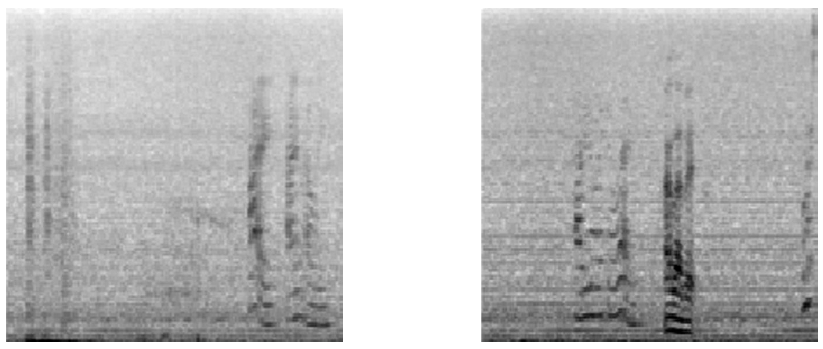
The 128-band Mel spectrograms are transformed to the decibel scale, normalized to the [0, 1] range, and saved as a grayscale image with a standardized resolution. These spectrogram images form the primary input to subsequent classification models (Figure 3).
The classification pipeline (Figure 2) begins by resizing spectrograms to a fixed input size. To address the severe class imbalance in depression labels, we apply SMOTE (Synthetic Minority Over-sampling Technique) to the spectrograms after flattening each 128 × 128 image into a 16,384-dimensional vector (Figure 4). This allows SMOTE to generate synthetic samples directly in the vector space. After oversampling, the vectors are reshaped back into spectrogram format. This approach addresses class imbalance while preserving the discriminative power of frequency-domain representations, which are empirically more effective for voice-based mental health analysis than raw waveforms. Similar SMOTE-based balancing strategies have been employed in recent speech-based depression detection studies using both spectrograms and acoustic feature vectors [15,22,23]. The balanced dataset is partitioned into stratified training and validation sets.

2.4. Neural Networks Architecture

The baseline architecture used in this study is a compact yet effective CNN tailored for audio-based binary classification (depressed vs. non-depressed). The network comprises 9 layers, counting all key operations such as convolution, activation, pooling, and the final fully connected output layer. This relatively shallow architecture was intentionally selected to ensure stable and interpretable ANN-to-SNN conversion while maintaining compatibility with spiking simulation constraints.
The architecture includes the following components:
  • Input Layer: 128 × 128 grayscale Mel-spectrograms (single-channel input)
  • Conv Layer 1: Conv2d(1, 32, kernel_size = 3) → ReLU activation
  • Pooling Layer 1: AvgPool2d(kernel_size = 2)
  • Conv Layer 2: Conv2d(32, 64, kernel_size = 3) → ReLU activation
  • Pooling Layer 2: AvgPool2d(kernel_size = 2)
  • Flattening Layer
  • Fully Connected Layer: Linear(128, 2) followed by softmax activation
No batch normalization or dropout was applied in order to preserve clarity in the CNN-to-SNN transformation and reduce conversion instability. The choice of average pooling over max pooling helps mitigate spike saturation during SNN simulation.
The model was trained using the cross-entropy loss function and optimized with the Adam optimizer, with default PyTorch parameters (β1 = 0.9, β2 = 0.999). A fixed learning rate of 1 × 10⁻³ was used throughout training. The training strategy included the following:
  • Batch size: 32
  • Early stopping: patience = 5 epochs, max epochs = 50
  • Average convergence epoch: 10
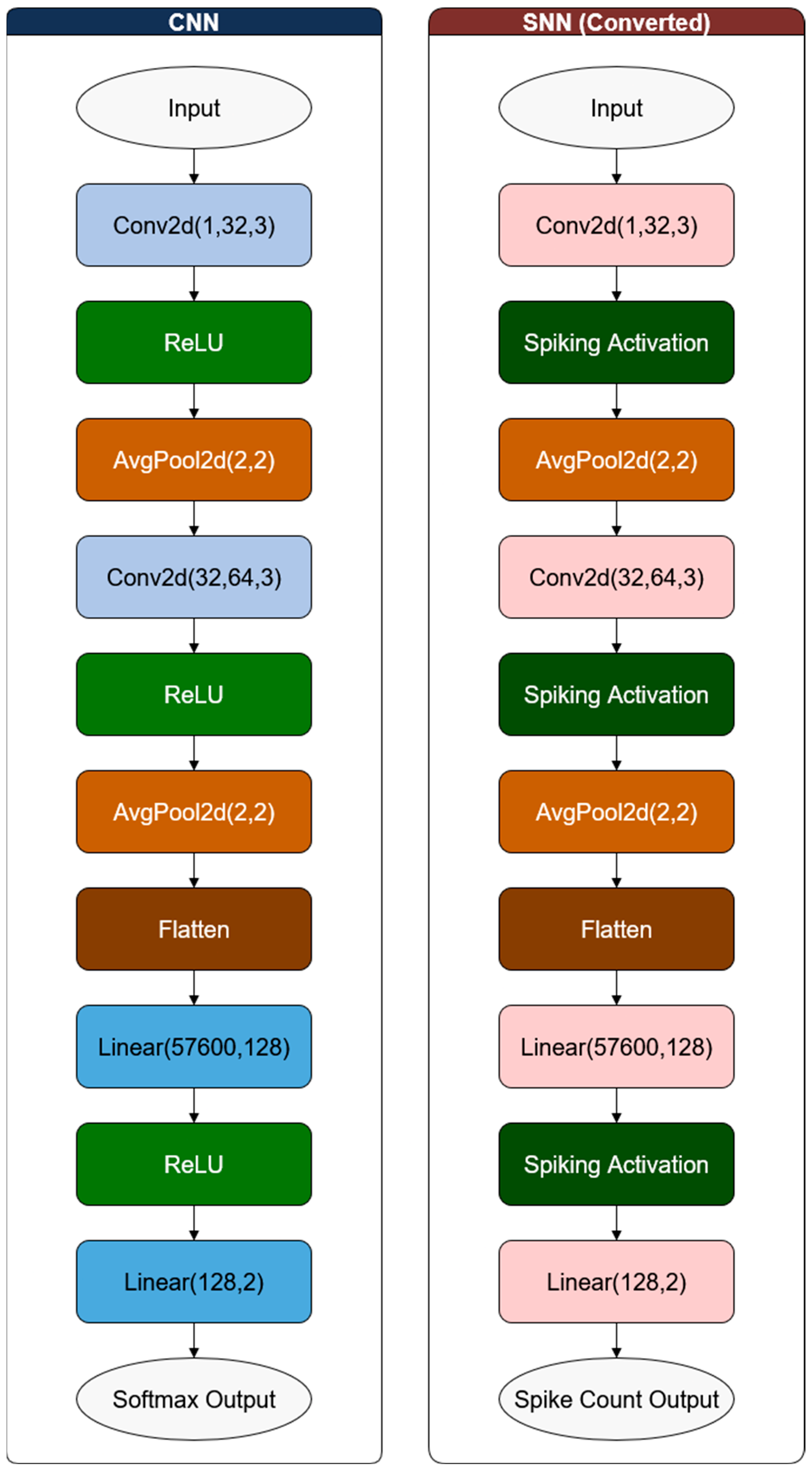
These design and training choices balance performance with interpretability and computational feasibility. The complete model architecture is visually summarized in Figure 5, and the same CNN was later converted into a spiking neural network using SpikingJelly’s ann2snn conversion module, as detailed in Section 3.
Figure 5 illustrates the architectural equivalence between the original CNN and the converted SNN models. Both networks follow an identical layer-wise structure: two convolutional layers (Conv2d(1, 32, 3) and Conv2d(32, 64, 3)), each followed by ReLU (in CNN) or spiking activation (in SNN) and AvgPool2d(2, 2) operations. After feature extraction, the data are flattened and passed through two fully connected layers—Linear(57600, 128) and Linear(128, 2)—culminating in a softmax output for the CNN and a spike count output for the SNN. This mirrored design ensures functional consistency and enables high-fidelity ANN-to-SNN conversion while maintaining interpretability and performance.
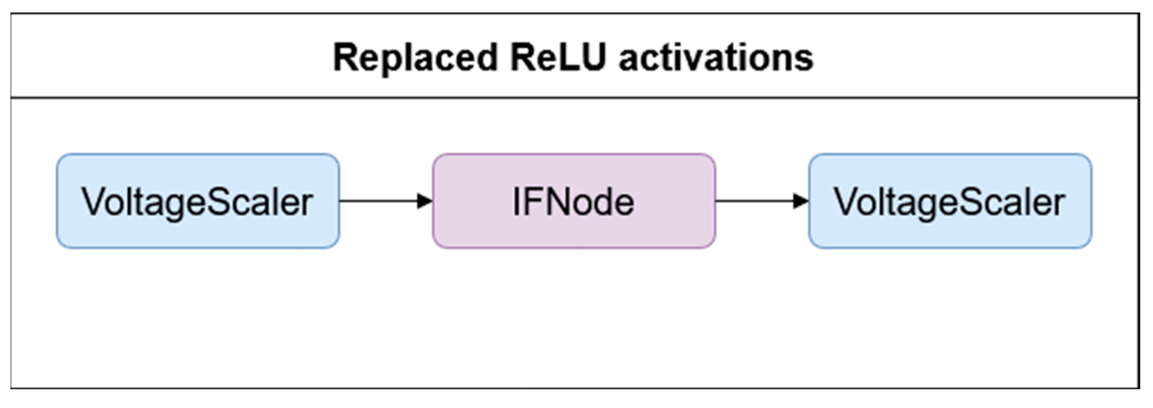
The trained CNN is converted into an SNN using SpikingJelly’s ANN-to-SNN converter [18]. The conversion process involves rate coding, layer-wise weight transfer, and threshold normalization (e.g., “max”, “99.9%” modes) to align the spiking neuron activity with the original activation statistics of the ANN. All ReLU activations are removed and replaced with modules consisting of a voltage scaler, an integrate-and-fire spiking neuron (IFNode), and another voltage scaler (Figure 6). These modules simulate spiking behavior and perform temporal integration over discrete time steps.
In the conversion process, we used the SpikingJelly framework to transform the trained CNN into an SNN via rate coding. This method encodes the ReLU activations of the CNN as spike rates in the SNN. Rather than using the absolute maximum activation value to scale these rates, we applied a percentile-based thresholding strategy. Specifically, the 99.9% mode refers to using the 99.9th percentile of all ReLU activations observed during training as the normalization denominator. This approach mitigates the influence of extreme outliers and results in more stable and biologically plausible firing rates. As illustrated in Figure 6, the input spectrogram is fed repeatedly into the SNN over T = 50 simulation time steps, during which each spiking neuron emits spikes proportionally to the original CNN activation, now interpreted as a firing rate. This allows the SNN to mimic the functional behavior of the CNN in a time-distributed, event-based manner suitable for neuromorphic deployment.
The original CNN architecture—comprising convolutional, pooling, flattening, and linear layers—is structurally preserved. However, the static non-linearities are replaced with dynamic, threshold-driven spiking units. The converted SNN operates over T simulation steps, and classification is performed by accumulating output spikes across time.
This conversion is not lossless: The SNN cannot fully replicate the behavior of the original CNN due to quantization artifacts, rate coding constraints, and the fundamental mismatch between continuous activations and discrete spike trains. As such, performance degradation is expected and must be evaluated empirically.
Due to the relatively limited size of the DAIC-WOZ dataset, all audio samples were merged and then randomly split into 80% for training and 20% for validation, using class stratification to preserve the proportion of depressed and non-depressed labels in both subsets. This approach ensured that both classes were adequately represented during model evaluation, while avoiding data leakage across participants.
The model was trained using the CrossEntropyLoss function, which is standard for binary classification problems involving a softmax output layer. We used the Adam optimizer with default PyTorch parameters (β1 = 0.9, β2 = 0.999) and a fixed learning rate of 1 × 10⁻³. The batch size was set to 32.
To prevent overfitting, early stopping was applied with a patience of 5 epochs and a maximum of 50 training epochs. In practice, the training consistently converged around epoch 10, indicating stable and efficient learning. No additional regularization methods, such as dropout or L2 weight decay, were used in order to preserve the fidelity of feature activations during the subsequent conversion to spiking neural networks.
These training conditions were kept consistent throughout all experiments to ensure reproducibility and allow for a clear assessment of the CNN-to-SNN conversion fidelity.
Model performance is measured by standard classification metrics, including accuracy, macro and micro F1 scores, ROC-AUC, precision, recall, specificity, negative predictive value, and confusion matrix statistics. Both the CNN and its spiking counterpart are subjected to identical evaluation protocols to enable direct comparison.
Initially, we explored direct training of spiking neural networks on spectrogram inputs using surrogate gradient-based methods, with variations in architecture depth, neuron types, simulation time steps, and learning rates. However, performance consistently remained in the range of 64–67% accuracy, with frequent instability. The key challenge stemmed from translating dense, continuous-valued spectrograms into spike-based representations without losing crucial frequency information. In contrast, converting a well-trained CNN using SpikingJelly’s ann2snn module preserved high accuracy (above 80%) and proved to be a more stable and scalable approach. Based on these findings, we adopted the conversion strategy as the core method for this study.
The primary motivation for converting a trained CNN to an SNN in this context is to investigate the feasibility of deploying more biologically plausible and energy-efficient computation methods for psychological signal classification. However, the overall system is constrained by several factors. The CNN architecture is deliberately simple, which may prevent it from capturing complex, nuanced patterns present in the data. Conversion may lead to performance degradation, often due to timing quantization and the limited expressiveness of current spiking encodings.

2.5. Software, Libraries, and Generative AI Tools

All experiments were conducted using Python v.3.12.5, with PyTorch v.2.5.1+cu121 serving as the primary deep learning framework for constructing and training the CNN model (torch, torch.nn, torch.utils.data), as well as managing GPU-accelerated computations. For SNN conversion and simulation, we used the SpikingJelly v.0.0.0.0.14 framework (spikingjelly.activation_based.ann2snn.Converter), which enables high-fidelity transformation from ANN to SNN models using rate coding. NumPy 2.1.3 and Pandas 2.2.3 were used for handling numerical arrays and tabular data, including dataset loading and manipulation. Audio spectrograms were preprocessed using Pillow 11.1.0 (PIL) for image loading and resizing. Scikit-learn 1.6.1 was employed for dataset splitting (train_test_split), classification evaluation (classification_report, confusion_matrix), and performance metric computation. To address class imbalance in the training data, we applied SMOTE from the imbalanced-learn 0.13.0 (imblearn) library. For visualization and result presentation, we used matplotlib 3.10.1 and seaborn 0.13.2, particularly for plotting confusion matrices and performance trends. This software stack ensured efficient training, evaluation, and reproducibility of both CNN and SNN models.
In the preparation of this manuscript, under the supervision of the authors, Microsoft 365 Copilot was used to assist with language refinement, enhance grammatical accuracy, and make clear the Abstract section, Section 1 and Section 5. It also assisted with the arrangement of tabular comparisons, standardizing methodological descriptions, and formatting the references to the journal style specifications. AI-generated content was never included without critical review and manual verification. All experimental design, data analysis, results interpretation, and conclusions are the intellectual contributions of the authors.

3. Results

All experiments were conducted on consumer-grade hardware: an NVIDIA GeForce RTX 4060 Ti GPU (NVIDIA, Santa Clara, CA, USA), AMD Ryzen 9 5900X 12-core CPU (Advanced Micro Devices, Inc. Santa Clara, CA, USA), and 64 GB RAM (Kingston Technology Corporation, Fountain Valley, CA, USA). The dataset used was DAIC-WOZ, processed into 128 × 128 Mel spectrograms as described previously. The SNNs were derived from a trained CNN using SpikingJelly’s ANN-to-SNN conversion pipeline. The simulation time for the SNNs was fixed at T = 50 time steps.

3.1. CNN Baseline Performance

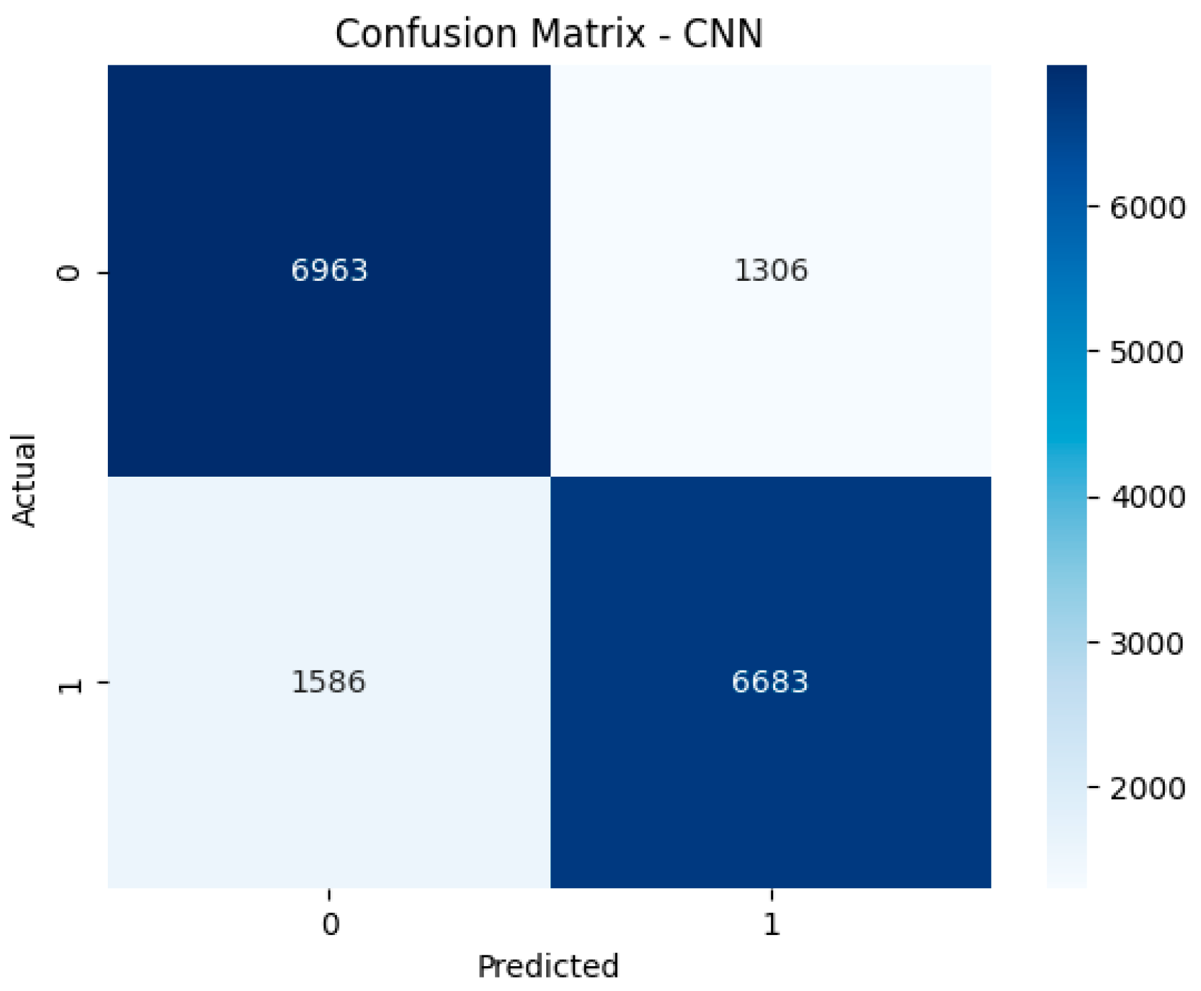
The baseline CNN achieved an accuracy of 82.51%, with a macro and micro F1 score of 0.8251, and an ROC-AUC of 0.9070. Class-wise metrics (Figure 7) show balanced precision and recall across classes:
  • Class 0 (Non-depressed): Precision = 0.8145, Recall = 0.8421, F1 = 0.8280
  • Class 1 (Depressed): Precision = 0.8365, Recall = 0.8082, F1 = 0.8221
These results indicate strong overall classification ability with high discriminative power, particularly evident in the ROC-AUC score.

3.2. SNN Performance Across Conversion Modes

Mode = max
This conversion method yielded the worst performance drop, with accuracy decreasing to 79.25% and ROC-AUC dropping to 0.8141. Recall for class 0 dropped significantly to 0.7038, suggesting that the SNN misclassified more non-depressed samples.
Mode = 99.9%
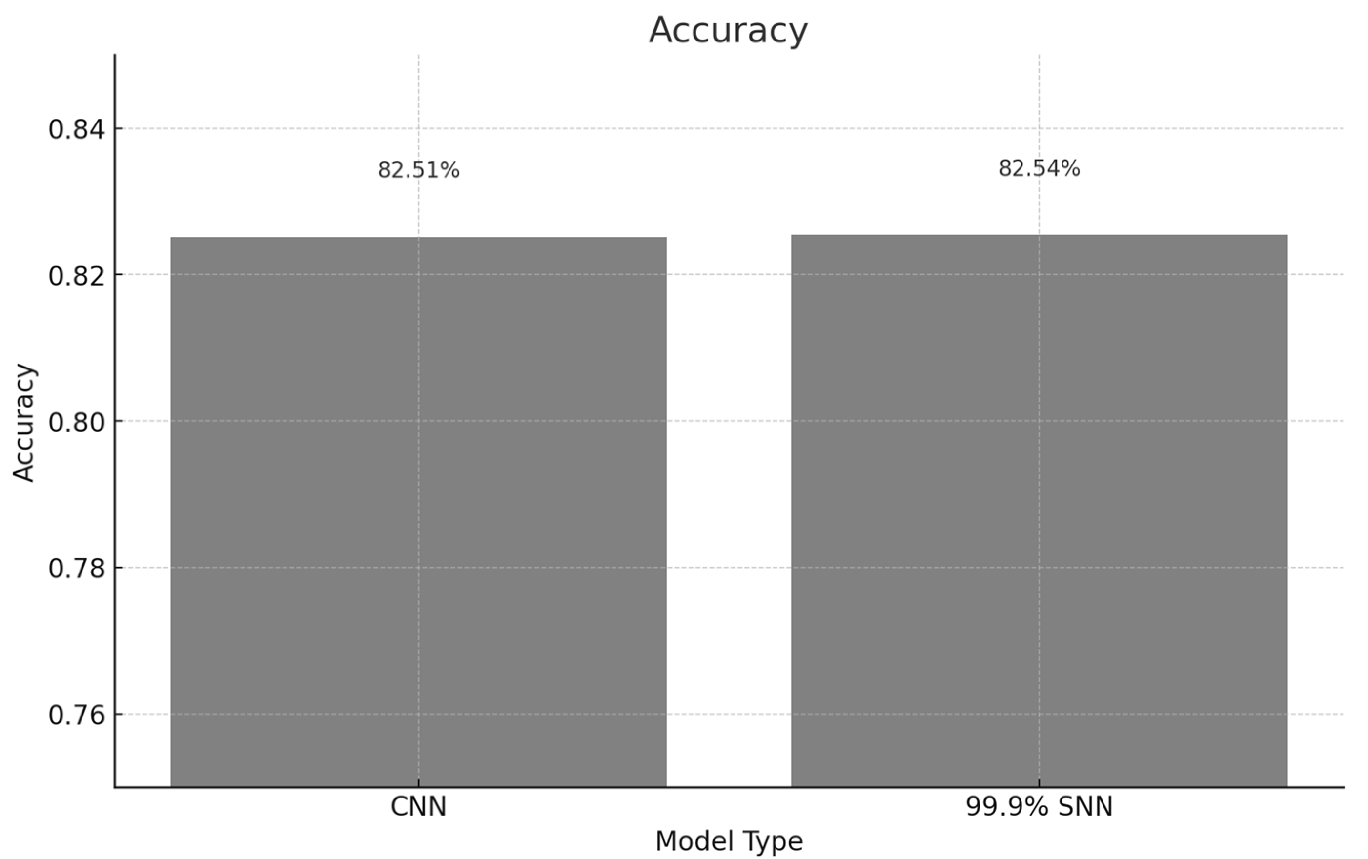
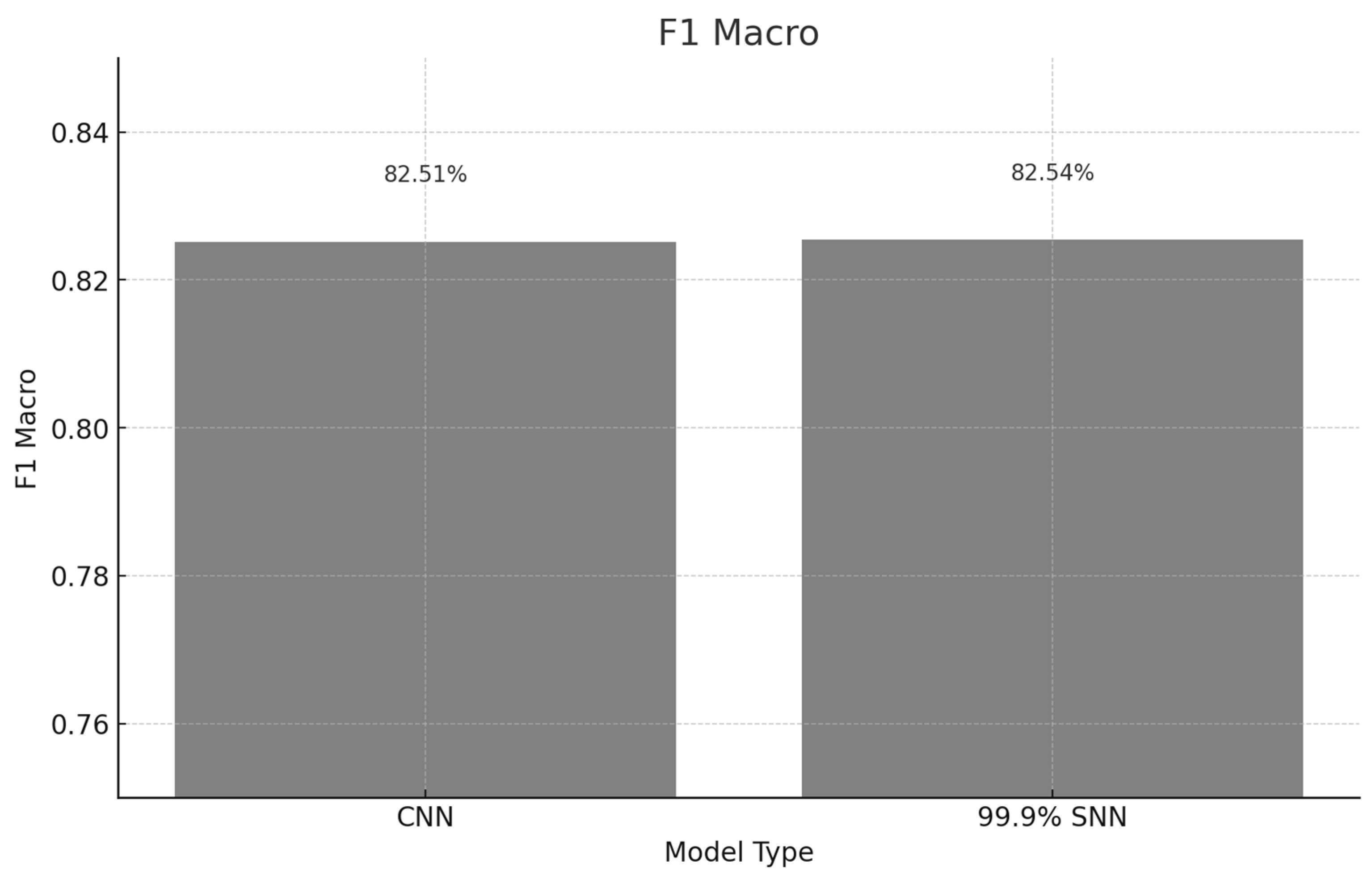
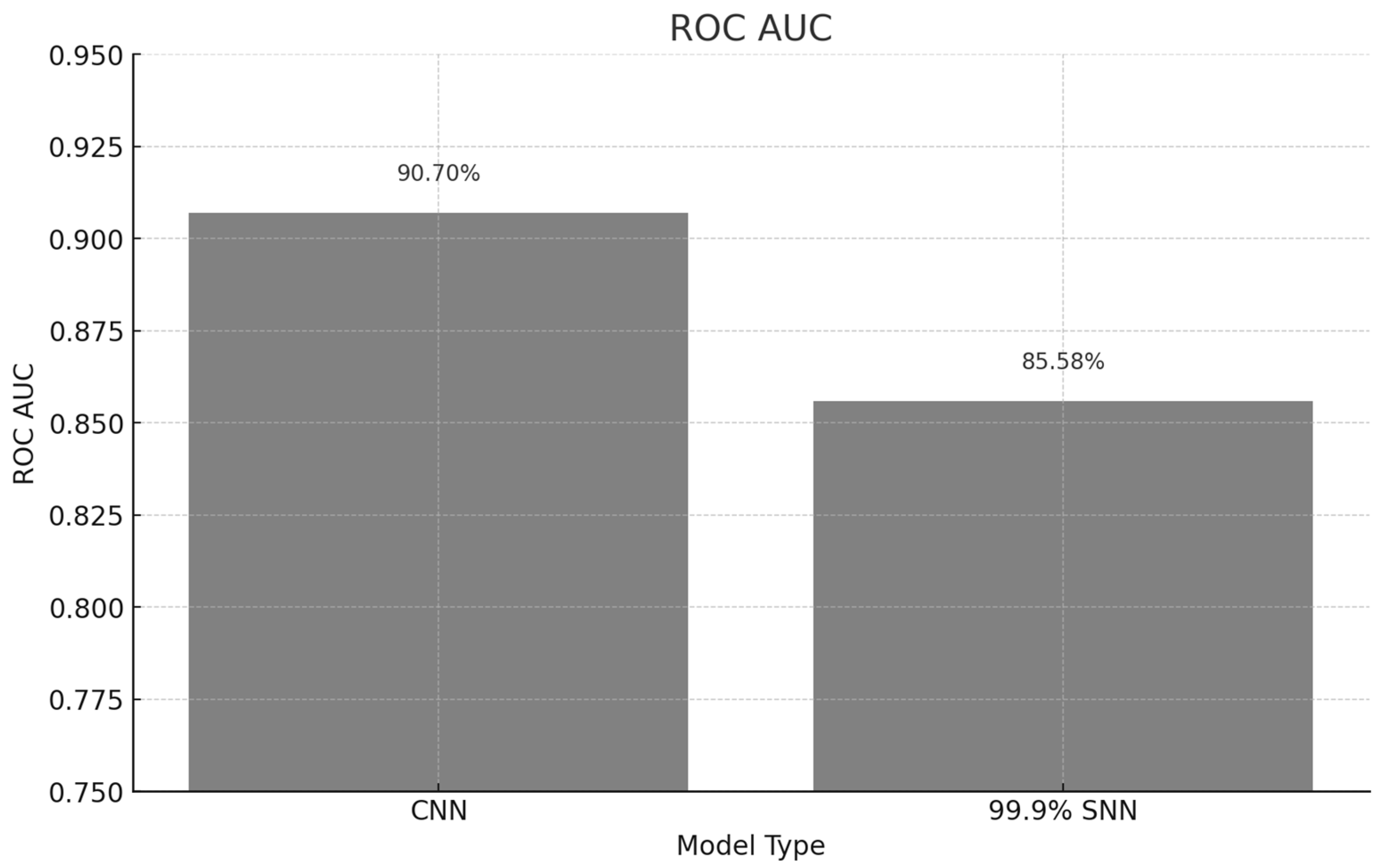
This mode showed no significant degradation, with accuracy at 82.54% and macro F1 of 0.8254—statistically equivalent to the CNN. ROC-AUC was slightly lower at 0.8558, but within acceptable variance. This suggests the 99.9% percentile threshold better aligns with the CNN’s activation statistics, preserving task performance.
Mode = 0.5 and 0.333
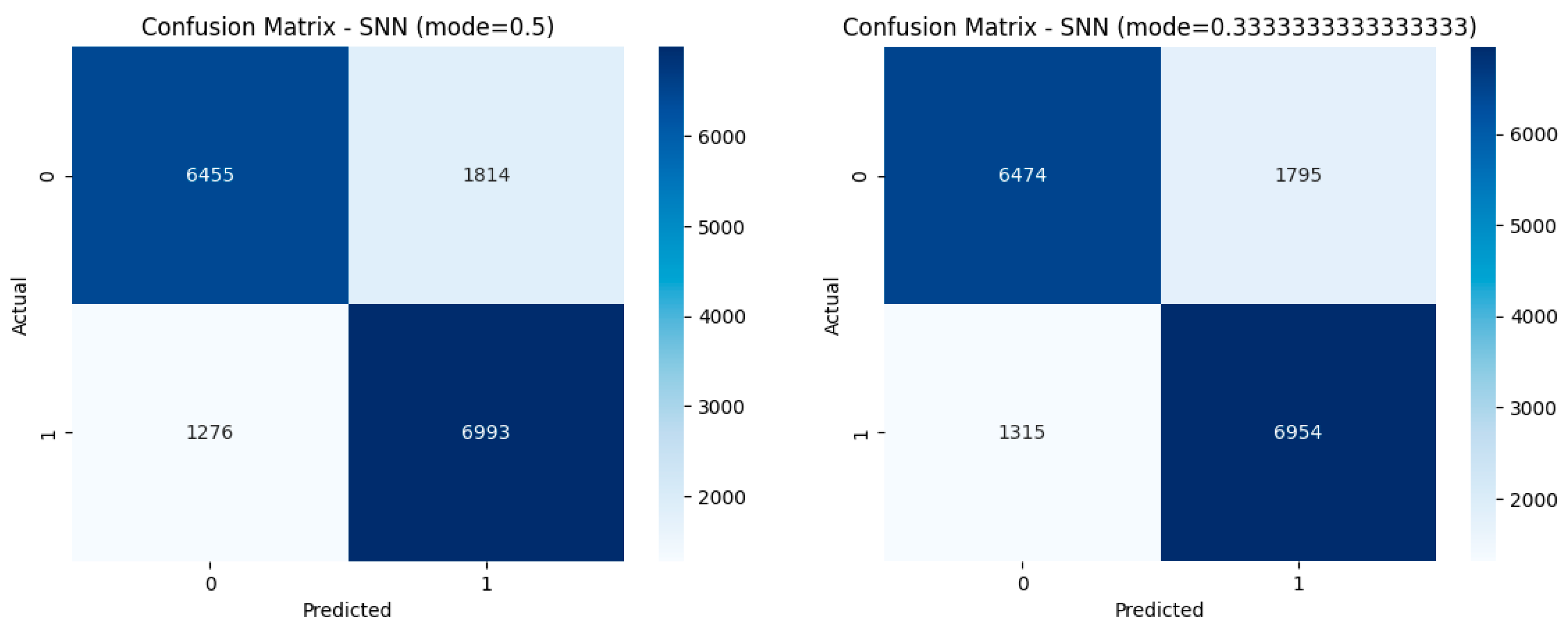
These lower-threshold conversions resulted in a moderate performance decrease (accuracy around 81.2–81.3%) (Figure 8). Interestingly, these SNNs had more balanced class-specific F1 scores (Figure 9) and improved recall for the depressed class, but slightly worse overall accuracy and ROC-AUC (Figure 10).
Table 2 presents the performance metrics of the baseline CNN model and several SNNs generated through the above conversion modes. Notably, the SNN obtained using the 99.9% conversion threshold delivers the most competitive results among the spiking architectures, closely matching the original CNN’s performance. It achieves an accuracy of 0.8254 and a macro F1 score of 0.8254—nearly identical to the CNN baseline (0.8251 for both). It also achieves balanced class-specific F1 scores (0.8285 for Class 0 and 0.8223 for Class 1) and maintains a high ROC-AUC of 0.8558, confirming strong discriminative power and minimal degradation from the ANN-to-SNN conversion process. A deeper examination of misclassification patterns reveals subtle but meaningful behavioral shifts across architectures. While the CNN is slightly biased toward classifying non-depressed cases (Class 0) more accurately, some SNN variants, particularly those using lower thresholds (0.5 and 0.333), improve sensitivity to the depressed class (Class 1) at the expense of specificity, leading to increased false positives. The max mode further amplifies this trade-off, reducing the Class 0 F1 score. These findings underscore that while overall accuracy and F1 scores may appear stable, conversion mode selection significantly impacts class-specific error tendencies. These results highlight the 99.9% conversion model as the most effective approach for preserving CNN-level diagnostic performance in SNN form, being the most promising solution for real-time, energy-efficient depression detection.

4. Discussion

4.1. Analysis and Interpretation

To better understand the influence of conversion parameters on SNN performance, we conducted a threshold-based evaluation across multiple configurations: 0.333, 0.5, 99.9%, and max mode. This systematic analysis serves as an ablation study on the conversion threshold component of the CNN-to-SNN pipeline. As shown in Table 2, different thresholds yield distinct trade-offs between overall accuracy, macro F1-score, and class-specific recall—particularly affecting sensitivity to the depressed class. This evaluation underscores the importance of precise conversion calibration in achieving reliable SNN-based classification and demonstrates how individual components contribute to the overall system performance.
The results of this study reveal both the promise and the challenges of converting CNNs into SNNs for audio-based depression detection. While the baseline CNN consistently outperformed or closely matched its converted SNN counterparts across most evaluation metrics, the quality of the conversion was highly dependent on the threshold parameter used during the process. Notably, the SNN converted using the 99.9% threshold retained nearly all of the CNN’s classification performance, achieving comparable accuracy, macro F1 score, and class-specific F1 metrics. This suggests that with careful calibration, ANN-to-SNN conversion can preserve high diagnostic fidelity, making SNNs viable for real-world deployment.
In contrast, the “max” conversion mode resulted in a significant degradation in performance, particularly in specificity for class 0 (non-depressed), indicating an overfitting to spiking behavior rather than to discriminative audio features (Figure 11). This finding underscores the sensitivity of SNN performance to conversion strategy and highlights the risk of naïve conversion approaches. SNNs generated using lower thresholds (0.5 and 0.333) showed slightly reduced overall accuracy but demonstrated increased recall for class 1 (depressed). Such a trade-off may be acceptable—or even preferable—in applications where identifying at-risk individuals is prioritized over minimizing false positives, as is often the case in mental health screening and early intervention scenarios.
All models were executed on standard GPU hardware using rate coding with a simulation window of 50 time steps (T = 50). This approach inherently introduces latency and computational overhead compared to feedforward CNNs. While this setup allowed for fair performance comparisons, it does not reflect the energy efficiency gains of SNNs when deployed on dedicated neuromorphic hardware. In practice, the event-driven nature of SNNs offers substantial benefits in power-constrained environments.

4.2. Comparative Analysis

Our results demonstrate strong performance in automated depression detection using CNN-based analysis of Mel spectrograms derived from DAIC-WOZ audio data (Table 3). With an F1-score of 0.8251 and ROC-AUC of 0.9070, our CNN outperforms or matches most prior works—even those employing more complex architectures or multimodal inputs. Furthermore, our spiking neural network (SNN) variant achieves comparable performance under the 99.9% threshold regime, with an F1-score of 0.8254 and accuracy of 82.54%, confirming the feasibility of ANN-to-SNN conversion in this context.
A direct comparison with Liu et al. [15] is particularly relevant, as both studies use DAIC-WOZ, apply Mel spectrograms, and employ CNNs. Liu et al. [15] reported an F1-score of 0.74 and accuracy of 0.73 in their monolingual English-only baseline. Despite similar preprocessing (5 s Mel spectrograms) and class imbalance handling (SMOTE), our CNN achieves significantly higher performance. This suggests that either our architectural simplicity generalizes better, or Liu et al.’s context-aware features introduce unnecessary complexity or overfitting.
In works using alternative CNN variants or forgoing spectrograms entirely, the comparisons become more nuanced. Manoret et al. [30] combined a 1D CNN with GRUs, reaching an F1-score of 0.75 using 1 s overlapping audio windows and Mel spectrograms. While theoretically more expressive, their additional complexity—via GRUs and stratified sampling—does not translate to superior performance.
Ding et al. [27] reported a high F1-score of 0.86 using an AMST (Audio Mel-Spectrogram Transformer). However, their approach differs significantly: It processes 50 s audio segments and employs a transformer-based architecture, offering richer temporal context.
Lin et al. [29] reported an F1-score of 0.81 for their audio-only 1D CNN. While their full model is multimodal, we isolate the audio-only metric for fairness. Their result is close to ours but does not surpass it, reinforcing the effectiveness of our 2D CNN architecture.
By contrast, Chlasta et al. [26] used 15 s spectrograms resized to 224 × 224 and a ResNet-34 with test-time augmentation (TTA), achieving an F1 of 0.6154—well below ours. Their accuracy (81%) is comparable, but the added complexity does not yield consistent gains, especially given DAIC-WOZ’s limited data.
Saeed et al. [24] reported 82.9% precision and 98.97% recall when combining MFCC and Mel spectrum features. However, using Mel alone, their CNN achieves only 79% accuracy without disclosing F1 or other metrics. This limits comparability. Regardless, our balanced metric profile suggests stronger reliability using only Mel spectrograms.
Older works like Hanai et al. [25] and Williamson et al. [33] are not directly comparable due to differing methodologies. Hanai’s audio-only sequence model yields an F1-score of 0.63, and Williamson’s best handcrafted feature-based model achieves an F1 of 0.57. These pioneering methods lack the representational power of modern CNN-based approaches.
Lam et al. [28] adopted a topic-segmented and augmented strategy using 1D CNNs, with their best F1-score at 0.67. Despite the clinical motivation of topic-awareness, generalization appears weaker than in our generic windowed approach.
Similarly, Saidi et al. [31] used 4 s spectrograms with a CNN and SVM hybrid, achieving an F1 of 0.67 and an accuracy of 58.57%. These results suggest limitations in both CNN backbone strength and feature transfer effectiveness—contrasting with the benefits of our end-to-end learning setup.
Vázquez-Romero et al. [32] reported only per-class metrics. Their best-case F1-score (0.76) falls short of ours. Despite using an ensemble of 1D CNNs with log-spectrograms, their results lack consistency across metrics and configurations.
Based on all the above, the comparative results presented in Table 3 demonstrate that our CNN model achieves competitive, and in several cases superior, performance compared to state-of-the-art approaches on the DAIC-WOZ dataset. Notably, while some transformer-based or multimodal methods report high recall or accuracy, they often involve more complex architectures, longer input windows, or additional modalities, which may limit their applicability in low-resource or real-time settings. Our 2D CNN architecture, combined with 5 s Mel spectrogram inputs and minimal preprocessing, offers a strong performance-to-complexity trade-off. More importantly, the successful conversion of this CNN into a high-fidelity SNN (under the 99.9% mode) with virtually no performance loss sets our approach apart from prior work, as it is the first to demonstrate that ANN-to-SNN conversion is feasible and effective for clinically relevant speech-based depression detection. This supports the potential of neuromorphic deployment in eHealth applications and strengthens the case for energy-efficient AI models in mental health assessment.

4.3. Future Directions

The key findings of this study demonstrate that SNNs can achieve performance comparable to conventional CNNs when the conversion process is carefully optimized. Specifically, the 99.9% conversion mode in SpikingJelly produced an SNN that matched the CNN’s accuracy (82.5%) and macro F1 score (0.8254), confirming that high-fidelity ANN-to-SNN conversion is feasible for real-world tasks such as depression detection from speech. In contrast, naïve conversion strategies—particularly the “max” mode—resulted in a marked decline in performance, with accuracy falling by more than 3% due to reduced recall for the non-depressed class. This underscores the fragility of SNN performance to conversion parameters. Furthermore, conversions using lower thresholds (such as 0.5 and 0.333) showed a trade-off pattern: Although they slightly lowered overall accuracy, they improved recall for the depressed class. These configurations may be especially useful in contexts where identifying at-risk individuals is more critical than avoiding false positives. Lastly, the conversion process was found to induce class-specific behavioral shifts in the models, altering the balance between precision and recall in an asymmetric way. This suggests that spike-based representations modify class boundaries differently from continuous activations and should be carefully considered in clinical applications.
Based on the above findings, future directions should include hybrid models that integrate audio with linguistic features, video or text processing, or adopt attention-based architectures, provided dataset limitations are mitigated through augmentation or access to larger corpora.
Additionally, testing the proposed approach on external datasets and validating its performance on newly collected real-world speech recordings will be essential to assess robustness and generalizability. Such efforts will address potential biases inherent in the DAIC-WOZ dataset, including demographic and environmental constraints.
Furthermore, the use of a deliberately shallow CNN architecture, while appropriate for controlled conversion analysis, limits the exploration of more expressive models; future work will address this by evaluating the scalability of the CNN-to-SNN conversion on deeper architectures with added regularization components. While this study relies on simulated SNNs executed on conventional GPU hardware, future work will include direct energy measurements on neuromorphic platforms such as Intel Loihi or IBM TrueNorth to validate real-world efficiency claims.
Although this study fixed the SNN simulation window at T = 50 time steps to balance resolution and cost, future work will include a systematic ablation study on the time-step budget to assess whether equivalent classification accuracy can be maintained under lower latency or reduced spike activity, which would provide more concrete insights into real-time efficiency trade-offs.
Nonetheless, our results demonstrate that carefully designed CNNs—combined with effective ANN-to-SNN conversion—can achieve strong performance while enabling deployment on energy-efficient, neuromorphic platforms. This establishes a viable path toward practical, low-power mental health monitoring systems.

5. Conclusions

Our CNN achieves state-of-the-art or near-state-of-the-art performance on DAIC-WOZ using only 5 s Mel spectrograms and a relatively simple architecture. It outperforms or matches more complex and multimodal models, establishing a robust baseline for depression detection with lightweight, explainable deep learning pipelines. The successful ANN-to-SNN conversion—with minimal performance degradation—extends its applicability to energy-efficient or neuromorphic computing platforms, which are critical for real-world deployment in low-power environments.
This study also has several limitations. The SNNs were simulated rather than deployed on actual neuromorphic hardware, preventing a direct assessment of real-world energy efficiency. The CNN architecture used for training and conversion was intentionally kept simple to ensure compatibility with existing SNN toolchains. A more complex architecture may yield different results, potentially exposing further limitations or strengths of the conversion process. The SpikingJelly framework assumes a clean transfer of activation distributions during conversion, an assumption that may not hold for deeper or highly nonlinear networks, which could compromise SNN fidelity in more advanced models.
Future research will aim to address the limitations identified in this study, including the need for evaluation on neuromorphic hardware and the exploration of more complex network architectures. Nevertheless, the present work contributes meaningfully to the expanding body of literature focused on bridging the gap between high-performance deep learning models and biologically inspired, energy-efficient architectures. The findings presented herein offer empirical support for the viability of properly configured SNNs as effective alternatives to CNNs in sensitive applications such as automated depression detection from speech data.

Author Contributions

Conceptualization, M.L. and A.C.I.; methodology, A.C.I.; software, V.T.; validation, M.L., V.T. and A.C.I.; formal analysis, M.L.; investigation, V.T.; resources, V.T.; data curation, V.T.; writing—original draft preparation, V.T.; writing—review and editing, M.L. and A.C.I.; visualization, M.L. and A.C.I.; supervision, M.L.; project administration, A.C.I.; funding acquisition, V.T. All authors have read and agreed to the published version of the manuscript.

Funding

This research received no external funding.

Institutional Review Board Statement

Ethical review and approval were waived for this study due to the policies of our university regarding exemption from ethical approval for studies involving publicly available anonymized datasets and no human subjects.

Informed Consent Statement

Not applicable.

Data Availability Statement

Data available upon request at https://dcapswoz.ict.usc.edu/ (accessed on 3 May 2024). All codes involved in obtaining the results presented in this paper are available at https://github.com/gv1x2/ANN2SNN-SpikingJelly- (accessed on 20 July 2025).

Acknowledgments

During the preparation of this manuscript, the authors used Microsoft 365 Copilot for the purposes of language editing, drafting assistance, and references’ formatting. The authors have reviewed and edited the output and take full responsibility for the content of this publication.

Conflicts of Interest

The authors declare no conflicts of interest.

References

  1. Leal, S.S.; Ntalampiras, S.; Sassi, R. Speech-Based Depression Assessment: A Comprehensive Survey. IEEE Trans. Affect. Comput. 2024, 1, 1–16. [Google Scholar] [CrossRef]
  2. Mao, K.; Wu, Y.; Chen, J. A Systematic Review on Automated Clinical Depression Diagnosis. Npj Ment. Health Res. 2023, 2, 20. [Google Scholar] [CrossRef]
  3. Moreno-Agostino, D.; Wu, Y.-T.; Daskalopoulou, C.; Hasan, M.T.; Huisman, M.; Prina, M. Global Trends in the Prevalence and Incidence of Depression: A Systematic Review and Meta-Analysis. J. Affect. Disord. 2021, 281, 235–243. [Google Scholar] [CrossRef]
  4. Brody, D.J.; Hughes, J.P. Depression Prevalence in Adolescents and Adults: United States, August 2021–August 2023. NCHS Data Brief 2025, 527, 1–11. [Google Scholar] [CrossRef]
  5. Terlizzi, E.P.; Zablotsky, B. Symptoms of Anxiety and Depression Among Adults: United States, 2019 and 2022. Natl. Health Stat. Rep. 2024, 213, CS353885. [Google Scholar]
  6. Arias-de la Torre, J.; Vilagut, G.; Ronaldson, A.; Bakolis, I.; Dregan, A.; Martín, V.; Martinez-Alés, G.; Molina, A.J.; Serrano-Blanco, A.; Valderas, J.M.; et al. Prevalence and Variability of Depressive Symptoms in Europe: Update Using Representative Data from the Second and Third Waves of the European Health Interview Survey (EHIS-2 and EHIS-3). Lancet Public Health 2023, 8, e889–e898. [Google Scholar] [CrossRef]
  7. Lim, G.Y.; Tam, W.W.; Lu, Y.; Ho, C.S.; Zhang, M.W.; Ho, R.C. Prevalence of Depression in the Community from 30 Countries between 1994 and 2014. Sci. Rep. 2018, 8, 2861. [Google Scholar] [CrossRef] [PubMed]
  8. Chen, Q.; Huang, S.; Xu, H.; Peng, J.; Wang, P.; Li, S.; Zhao, J.; Shi, X.; Zhang, W.; Shi, L.; et al. The Burden of Mental Disorders in Asian Countries, 1990–2019: An Analysis for the Global Burden of Disease Study 2019. Transl. Psychiatry 2024, 14, 167. [Google Scholar] [CrossRef] [PubMed]
  9. Mahmud, S.; Mohsin, M.; Dewan, M.N.; Muyeed, A. The Global Prevalence of Depression, Anxiety, Stress, and Insomnia Among General Population During COVID-19 Pandemic: A Systematic Review and Meta-Analysis. Trends Psychol. 2023, 31, 143–170. [Google Scholar] [CrossRef]
  10. Jia, H.; Guerin, R.J.; Barile, J.P.; Okun, A.H.; McKnight-Eily, L.; Blumberg, S.J.; Njai, R.; Thompson, W.W. National and State Trends in Anxiety and Depression Severity Scores Among Adults During the COVID-19 Pandemic—United States, 2020–2021. MMWR Morb. Mortal. Wkly. Rep. 2021, 70, 1427–1432. [Google Scholar] [CrossRef] [PubMed]
  11. Kroenke, K.; Strine, T.W.; Spitzer, R.L.; Williams, J.B.W.; Berry, J.T.; Mokdad, A.H. The PHQ-8 as a Measure of Current Depression in the General Population. J. Affect. Disord. 2009, 114, 163–173. [Google Scholar] [CrossRef]
  12. Lu, Y.-J.; Chang, X.; Li, C.; Zhang, W.; Cornell, S.; Ni, Z.; Masuyama, Y.; Yan, B.; Scheibler, R.; Wang, Z.-Q.; et al. ESPnet-SE++: Speech Enhancement for Robust Speech Recognition, Translation, and Understanding. In Proceedings of the Interspeech 2022, Incheon, Republic of Korea, 18–22 September 2022; pp. 5458–5462. [Google Scholar] [CrossRef]
  13. Wu, P.; Wang, R.; Lin, H.; Zhang, F.; Tu, J.; Sun, M. Automatic Depression Recognition by Intelligent Speech Signal Processing: A Systematic Survey. CAAI Trans. Intell. Technol. 2023, 8, 701–711. [Google Scholar] [CrossRef]
  14. Othmani, A.; Kadoch, D.; Bentounes, K.; Rejaibi, E.; Alfred, R.; Hadid, A. Towards Robust Deep Neural Networks for Affect and Depression Recognition from Speech. In Pattern Recognition. ICPR International Workshops and Challenges; Lecture Notes in Computer Science; Springer: Cham, Switzerland, 2021; Volume 12662, pp. 5–19. [Google Scholar] [CrossRef]
  15. Liu, L.; Liu, L.; Wafa, H.A.; Tydeman, F.; Xie, W.; Wang, Y. Diagnostic Accuracy of Deep Learning Using Speech Samples in Depression: A Systematic Review and Meta-Analysis. J. Am. Med. Inform. Assoc. 2024, 31, 2394–2404. [Google Scholar] [CrossRef]
  16. Kapse, P.; Garg, V.K. Advanced Deep Learning Techniques for Depression Detection: A Review. SSRN Sch. Pap. 2022, 4180783. [Google Scholar] [CrossRef]
  17. Boulal, H.; Hamidi, M.; Abarkan, M.; Barkani, J. Amazigh CNN Speech Recognition System Based on Mel Spectrogram Feature Extraction Method. Int. J. Speech Technol. 2024, 27, 287–296. [Google Scholar] [CrossRef]
  18. Fang, W.; Chen, Y.; Ding, J.; Yu, Z.; Masquelier, T.; Chen, D.; Huang, L.; Zhou, H.; Li, G.; Tian, Y. SpikingJelly: An Open-Source Machine Learning Infrastructure Platform for Spike-Based Intelligence. Sci. Adv. 2023, 9, eadi1480. [Google Scholar] [CrossRef]
  19. Bu, T.; Fang, W.; Ding, J.; Dai, P.; Yu, Z.; Huang, T. Optimal ANN-SNN Conversion for High-Accuracy and Ultra-Low-Latency Spiking Neural Networks. arXiv 2023. [Google Scholar]
  20. Izhikevich, E.M. Simple Model of Spiking Neurons. IEEE Trans. Neural Netw. 2003, 14, 1569–1572. [Google Scholar] [CrossRef] [PubMed]
  21. Gratch, J.; Artstein, R.; Lucas, G.; Stratou, G.; Scherer, S.; Nazarian, A.; Wood, R.; Boberg, J.; DeVault, D.; Marsella, S.; et al. The Distress Analysis Interview Corpus of Human and Computer Interviews. In Proceedings of the Ninth International Conference on Language Resources and Evaluation (LREC’14), Reykjavik, Iceland, 26–31 May 2014; pp. 3123–3128. [Google Scholar]
  22. Pandya, S. A Machine Learning Framework for Enhanced Depression Detection in Mental Health Care Setting. Int. J. Sci. Res. Sci. Eng. Technol. 2023, 10, 356–368. [Google Scholar] [CrossRef]
  23. Bhatt, N.; Jain, A.; Jain, M.; Bhatt, S. Depression Detection from Speech Using a Voting Ensemble Approach. In Proceedings of the 2024 IEEE 8th International Conference on Information and Communication Technology (CICT), Allahabad, India, 21–23 March 2024; pp. 1–6. [Google Scholar] [CrossRef]
  24. Saeed, M.; Komashinsky, V.; Mohammed, S.; Abdulqader, N.; Saif, L. Speech Signal Analysis to Predict Depression. Int. J. Adv. Netw. Appl. 2025, 16, 6460–6465. [Google Scholar] [CrossRef]
  25. Al Hanai, T.; Ghassemi, M.; Glass, J. Detecting Depression with Audio/Text Sequence Modeling of Interviews. In Proceedings of the Interspeech 2018, Hyderabad, India, 2–6 September 2018; pp. 1716–1720. [Google Scholar] [CrossRef]
  26. Chlasta, K.; Wołk, K.; Krejtz, I. Automated Speech-Based Screening of Depression Using Deep Convolutional Neural Networks. Procedia Comput. Sci. 2019, 164, 618–628. [Google Scholar] [CrossRef]
  27. Ding, H.; Du, Z.; Wang, Z.; Xue, J.; Wei, Z.; Yang, K.; Jin, S.; Zhang, Z.; Wang, J. IntervoxNet: A Novel Dual-Modal Audio-Text Fusion Network for Automatic and Efficient Depression Detection from Interviews. Front. Phys. 2024, 12, 1430035. [Google Scholar] [CrossRef]
  28. Lam, G.; Dongyan, H.; Lin, W. Context-Aware Deep Learning for Multi-Modal Depression Detection. In Proceedings of the ICASSP 2019—2019 IEEE International Conference on Acoustics, Speech and Signal Processing (ICASSP), Brighton, UK, 12–17 May 2019; IEEE: Piscataway, NJ, USA, 2019. [Google Scholar] [CrossRef]
  29. Lin, L.; Chen, X.; Shen, Y.; Zhang, L. Towards Automatic Depression Detection: A BiLSTM/1D CNN-Based Model. Appl. Sci. 2020, 10, 8701. [Google Scholar] [CrossRef]
  30. Manoret, P.; Chotipurk, P.; Sunpaweravong, S.; Jantrachotechatchawan, C.; Duangrattanalert, K. Automatic Detection of Depression from Stratified Samples of Audio Data. arXiv 2021. [Google Scholar] [CrossRef]
  31. Saidi, A.; Ben Othman, S.; Ben Saoud, S. Hybrid CNN-SVM Classifier for Efficient Depression Detection System. In Proceedings of the 2020 4th International Conference on Advanced Systems and Emergent Technologies (IC_ASET), Hammamet, Tunisia, 19–22 March 2020; IEEE: Piscataway, NJ, USA, 2020; pp. 229–234. [Google Scholar] [CrossRef]
  32. Vázquez-Romero, A.; Gallardo-Antolín, A. Automatic Detection of Depression in Speech Using Ensemble Convolutional Neural Networks. Entropy 2020, 22, 688. [Google Scholar] [CrossRef] [PubMed]
  33. Williamson, J.R.; Godoy, E.; Cha, M.; Schwarzentruber, A.; Khorrami, P.; Gwon, Y.; Kung, H.-T.; Dagli, C.; Quatieri, T.F. Detecting Depression Using Vocal, Facial and Semantic Communication Cues. In Proceedings of the 6th International Workshop on Audio/Visual Emotion Challenge (AVEC ‘16), Amsterdam, The Netherlands, 16 October 2016; Association for Computing Machinery: New York, NY, USA, 2016; pp. 11–18. [Google Scholar] [CrossRef]
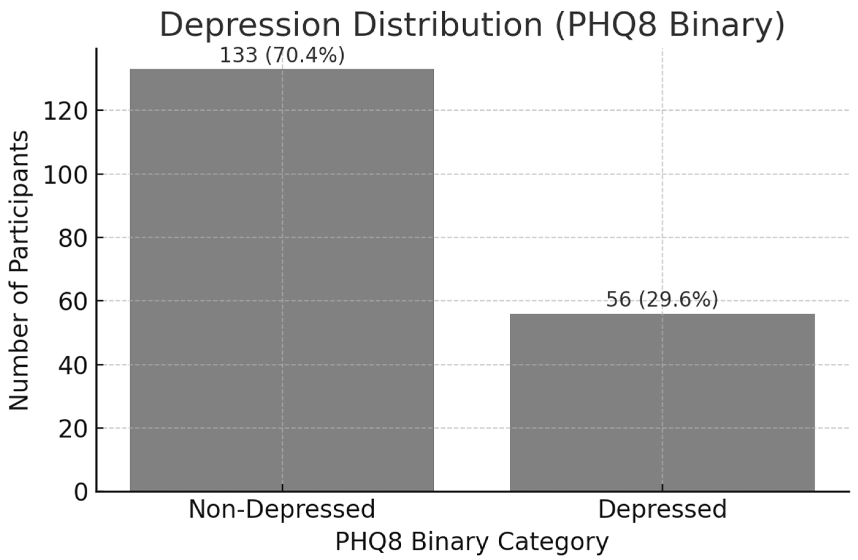
Figure 1. Dataset structure.
Applsci 15 09032 g001
Figure 2. Research diagram.
Applsci 15 09032 g002
Figure 3. Initial spectrograms.
Applsci 15 09032 g003
Figure 4. Resized spectrograms.
Applsci 15 09032 g004
Figure 5. CNN vs. SNN structure.
Applsci 15 09032 g005
Figure 6. ReLU activation replacement in SNN.
Applsci 15 09032 g006
Figure 7. Confusion matrix for CNN.
Applsci 15 09032 g007
Figure 8. SNN accuracy across modes.
Applsci 15 09032 g008
Figure 9. SNN F1 macro across modes.
Applsci 15 09032 g009
Figure 10. SNN ROC AUC across modes.
Applsci 15 09032 g010
Figure 11. Confusion matrix comparison.
Applsci 15 09032 g011aApplsci 15 09032 g011b
Table 1. Comparison between CNNs and SNNs.
AspectCNNSNN
Data typeContinuous (real-valued)Discrete (spikes over time)
Time dynamicsStatic inputTemporal input/output
Energy efficiencyLow (power-hungry inference)High (sparse, event-driven)
Training methodStandard backpropagationSurrogate gradients, ANN-to-SNN conversion
Biological realismLowHigh
Use case maturityProduction-ready, standardizedExperimental, emerging
Table 2. All models resulted metrics.
ModelAccuracyMacro F1ROC-AUCClass 0 F1Class 1 F1
CNN0.82510.82510.90700.82800.8221
SNN (max)0.79250.79090.81410.77230.8094
SNN (99.9%)0.82540.82540.85580.82850.8223
SNN (0.5)0.81320.81300.83820.80690.8190
SNN (0.333)0.81190.81180.84070.80630.8173
Bold highlights the best results.
Table 3. Comparative analysis.
MethodPrecisionRecallF1-ScoreAccuracyOther MetricsReference
MFCC + Mel spectrum82.90%98.97%91.43%82%
79% *
[24]
Sequence (Audio)0.710.560.63[25]
ResNet 34 (224 × 224 px)0.57140.66670.615481%[26]
CNN (audio)0.800.920.860.79[27]
CNN-Augm (audio)0.780.580.67[28]
1D CNN (audio)0.730.920.81[29]
Monolingual (DAIC WOZ)0.700.780.740.73Specificity: 0.68[15]
1D CNN-GRU64.0091.6775.00[30]
CNN0.550.860.6758.57[31]
1D-CNN (1,5 kernel size)0.50 (0.85)0.72 (0.69)0.59 (0.76)0.70 (0.70)[32]
Audio fusion 0.57AUC: 0.72[33]
CNN (Our work)0.81450.84210.82510.8251ROC-AUC: 0.9070This work
SNN (99.9%, Our work)0.82850.80820.82540.8254ROC-AUC: 0.8558This work
* Mel spectrum alone. Bold highlights our results.
Disclaimer/Publisher’s Note: The statements, opinions and data contained in all publications are solely those of the individual author(s) and contributor(s) and not of MDPI and/or the editor(s). MDPI and/or the editor(s) disclaim responsibility for any injury to people or property resulting from any ideas, methods, instructions or products referred to in the content.