Article

CAESAR: A Unified Framework for Foundation and Generative Models for Efficient Compression of Scientific Data

1
Department of Computer & Information Science & Engineering, University of Florida, Gainesville, FL 32611, USA
2
Oak Ridge National Laboratory, Oak Ridge, TN 37830, USA
*
Authors to whom correspondence should be addressed.
Appl. Sci. 2025, 15(16), 8977; https://doi.org/10.3390/app15168977 (registering DOI)
Submission received: 8 July 2025 / Revised: 6 August 2025 / Accepted: 10 August 2025 / Published: 14 August 2025
(This article belongs to the Section Computing and Artificial Intelligence)

Abstract

We introduce CAESAR, a new framework for scientific data reduction that stands for Conditional AutoEncoder with Super-resolution for Augmented Reduction. The baseline model, CAESAR-V, is built on a standard variational autoencoder with scale hyperpriors and super-resolution modules to achieve high compression. It encodes data into a latent space and uses learned priors for compact, information-rich representations. The enhanced version, CAESAR-D, begins by compressing keyframes using an autoencoder and extends the architecture by incorporating conditional diffusion to interpolate the latent spaces of missing frames between keyframes. This enables high-fidelity reconstruction of intermediate data without requiring their explicit storage. By distinguishing CAESAR-V (variational) from CAESAR-D (diffusion-enhanced), we offer a modular family of solutions that balance compression efficiency, reconstruction accuracy, and computational cost for scientific data workflows. Additionally, we develop a GPU-accelerated postprocessing module which enforces error bounds on the reconstructed data, achieving real-time compression while maintaining rigorous accuracy guarantees. Experimental results across multiple scientific datasets demonstrate that our framework achieves up to 10× higher compression ratios compared to rule-based compressors such as SZ3. This work provides a scalable, domain-adaptive solution for efficient storage and transmission of large-scale scientific simulation data.

1. Introduction

Foundation models (FMs) have gained significant traction across a range of domains due to their adaptability, scalability, and ability to generalize across tasks. Landmark models such as SAM [1] have demonstrated the power of transfer learning by pretraining on large, diverse datasets and fine-tuning for specific applications. However, the application of such high-capacity models in scientific data compression remains largely unexplored.
Scientific simulations executed on high-performance computing (HPC) systems routinely generate massive, high-resolution spatiotemporal datasets, placing tremendous strain on storage, transmission, and downstream analysis pipelines [2,3,4]. Existing lossy compressors—including wavelet transforms, tensor decompositions, and rule-based techniques such as SZ3 [5]—while effective in certain contexts, often struggle to preserve the intricate spatiotemporal correlations and high-dimensional structures essential for scientific analysis, especially when strict error-bound guarantees are required.
Recent machine learning-based approaches have shown promise in this space, particularly for domain-specific compression. Prior work [4] introduced models for scientific data compression built on attention mechanisms over tensor hyper-blocks, learning latent representations while enforcing error bounds on primary data (PD) and quantities of interest (QoI). However, these efforts have primarily focused on transform-based techniques, applying autoencoders, quantization, and entropy coding independently to spatial or spatiotemporal tensor blocks, limiting their adaptability and compression efficiency in dynamic or multi-domain simulation settings.
In this paper, we take a significant step forward by proposing two complementary foundation frameworks for scalable, high-fidelity scientific data reduction rooted in CAESAR (https://github.com/Shaw-git/CAESAR (accessed on 11 August 2025)) (Conditional AutoEncoder with Super-resolution for Augmented Reduction), comprising latent space embeddings, learned quantization, super-resolution and error bound guarantees:
  • A transform-based foundation model, combining a variational autoencoder (VAE) with hyper-prior structures and an integrated super-resolution (SR) module, referred to as CAESAR-V. The VAE captures latent space dependencies for efficient transform-based compression, while the SR module enhances reconstruction quality by refining low-resolution outputs. Alternating between 2D and 3D convolutions allows the model to efficiently capture spatiotemporal correlations at low computational cost.
  • A generative foundation model, named CAESAR-D, that integrates transform-based compression for keyframes with generative diffusion-driven temporal interpolation across data blocks. Our method employs a variational autoencoder (VAE) paired with a hyperprior to compress selected keyframes into compact latent representations. These latent codes are not only used to reconstruct the corresponding keyframes but also to condition a conditional diffusion (CD) model tasked with generating the missing intermediate blocks. The CD model begins from noisy inputs for non-keyframe positions and iteratively denoises them, using the latent embeddings of neighboring keyframes as auxiliary context. This framework achieves high compression efficiency while preserving strict reconstruction accuracy by statistically inferring intermediate frames in a data-consistent, generative manner.
The transform-based model provides faster performance due to its streamlined encoding and decoding process. The generative model achieves superior compression ratios but incurs higher computational cost because of the iterative diffusion steps involved in reconstruction. Crucially, both foundation frameworks are pretrained on a collection of diverse scientific datasets spanning multiple domains, enabling them to learn generalizable representations of spatiotemporal scientific phenomena. This pretraining strategy delivers more than 2× higher compression ratios than state-of-the-art rule-based compressors without domain-specific tuning. Furthermore, when fine-tuned on specific scientific datasets, the proposed models achieve an additional 1.5–5× improvement in compression ratio, outperforming state-of-the-art scientific compressors under the same reconstruction error constraints.
Furthermore, we introduce a post-processing module that enforces strict error-bound guarantees on the reconstructed primary data, ensuring that lossy compression does not compromise downstream analyses or simulations requiring quantifiable accuracy. To enhance its practicality, we implement a GPU-parallelized version of this post-processing step, achieving throughput of 0.4 1.1 GB / s , depending on the user-defined error bound. This capability makes the overall framework suitable for deployment in HPC environments where both compression fidelity and speed are critical.
This work builds upon and substantially extends our prior study [6], which focused solely on conditional latent diffusion for spatiotemporal interpolation. Here, we propose a unified and deployable framework that integrates learned transform-based compression (CAESAR-V), generative reconstruction via latent diffusion (CAESAR-D), and a GPU-parallelized postprocessing module that ensures strict error-bound guarantees. This integration offers both high compression ratios and accurate reconstructions across diverse scientific datasets.
We evaluate these two foundation models across multiple scientific domains—including E3SM [7], S3D [8], and JHTDB [9]—and benchmark their performance against state-of-the-art compression methods. Results demonstrate that our models achieve up to 3 10 × higher compression ratios at the same reconstruction error compared to other compressors.
The key contributions of this work are summarized as follows:
  • We propose two complementary foundation frameworks for scientific data compression: (i) a transform-based model combining a variational autoencoder (VAE) with hyperprior structures and a super-resolution (SR) module, and (ii) a generative model based on conditional latent diffusion for learned spatiotemporal interpolation across data blocks.
  • We incorporate a GPU-parallelized post-processing module that enforces user-specified error-bound guarantees on the reconstructed primary data, achieving throughput of 0.4 GB/s to 1.1 GB/s, thereby supporting scientific applications demanding quantifiable accuracy.
  • To improve the efficiency and scalability of the generative model, we fine-tune the diffusion process to operate with significantly fewer denoising steps, ensuring its applicability to large-scale and real-time scientific workflows.
  • Both foundation models are pretrained on diverse multi-domain scientific datasets, achieving more than 2× higher compression ratios than state-of-the-art rule-based compressors without domain-specific tuning. Further fine-tuning on target datasets yields an additional 1.5–5× improvement in compression ratio while preserving strict reconstruction error guarantees.

2. Related Work

Rule-based compression methods reduce data size using predefined mathematical models without requiring large training datasets. For example, ZFP [10] partitions data into 4D blocks and applies a near-orthogonal transform to decorrelate values. TTHRESH [11] leverages higher-order singular value decomposition (HOSVD) to retain only the most significant components, effectively reducing dimensionality. MGARD [12,13] employs a multigrid-based approach, representing data as a hierarchy of coefficients to enable multi-resolution analysis and controllable error bounds. Classical methods also improve compressibility by predicting values from neighboring points. For instance, Differential Pulse Code Modulation (DPCM) [14] encodes differences between successive samples, while MPEG standards [15] estimate unknown values through interpolation. Note that while DPCM and MPEG are primarily developed for human visual perception, we include them here to provide conceptual background. Our method, by contrast, targets scientific data where numerical fidelity and strict error bounds are essential. The widely adopted SZ compressor [16] enhances prediction accuracy by exploiting local data, with multiple variants tailored for different scenarios. More recently, FAZ [17] combines predictive models and wavelet transforms in a modular design for adaptable and efficient compression. Although these techniques are typically fast, their compression ratios generally remain lower than those achieved by modern machine learning–based methods.
On the other hand, learning-driven compression techniques have recently shown considerable promise for lossy compression, especially in maintaining reconstruction quality. Variational Autoencoders (VAEs) [18] and their advancements [19,20] have pushed the boundaries in this domain. For example, Ref. [19] merges autoregressive components with hierarchical priors to create context-aware latent predictions guided by a hyperprior autoencoder. The study in [20] further extends VAE models by integrating super-resolution modules and alternating 2D and 3D convolutions, effectively capturing spatiotemporal features and yielding high compression ratios alongside fine reconstructions. Meanwhile, Ref. [4] introduces a block-based compression method utilizing self-attention to better model both local and cross-block relationships within the data.
Diffusion models have recently demonstrated impressive capabilities in image generation applications [21,22]. Conditional variants [6,23] have gained attention for leveraging auxiliary information to guide the generative process, where such information can act as a compressed form of the original data. Diffusion models introduce a set of hierarchical latent variable models that generate data by iteratively reversing a sequence of noise-adding transformations [24,25,26]. These models define a joint distribution over data x 0 and latent variables x 1 : T , where the latter represents intermediate noisy versions of the data. The generative process starts from a latent representation drawn from a simple prior (e.g., Gaussian noise) and progressively refines it to produce structured data, such as images. The forward process q systematically adds random noise to the data eroding structure until the data becomes nearly indistinguishable from pure noise:
q x t | x t 1 = N x t | 1 β t x t 1 , β t I ,
where β t is a predefined or learned noise schedule. The reverse process p θ uses a neural network to iteratively recover the data by predicting the denoised states:
p θ x t 1 | x t = N x t 1 | M θ x t , t , β t I .
The reverse process is trained to approximate the true denoising transitions by minimizing a noise-prediction objective. Specifically, the model predicts the added noise ϵ for a given noisy sample x t , and the loss function is defined as
L θ , x 0 = E ϵ ϵ θ x t , t 2 ,
where x t is constructed as x t = α ¯ t x 0 + 1 α ¯ t ϵ , α t = 1 β t , and α ¯ t = s = 1 t α s . By leveraging this objective, the model learns to reverse the forward process and restore data from noise effectively.
For sampling, the reverse process can follow a stochastic trajectory, as in Denoising Diffusion Probabilistic Models (DDPMs) [26], or a deterministic path, as in Denoising Diffusion Implicit Models (DDIMs) [27]. The deterministic approach enables faster generation while retaining high-quality results, making it practical for tasks where efficiency is critical.
Conditional diffusion models for compression extend diffusion models to lossy data compression by leveraging conditional generation [28]. In this framework, an image x 0 is compressed into a set of latent representations z using an entropy-optimized quantization process. These latent variables are then used as conditioning inputs to guide the reverse diffusion process:
p θ x t 1 | x t , z = N x t 1 | M θ x t , z , t , β t I .
Here, z captures content information about an image, while the reverse diffusion process reconstructs finer texture details progressively. This approach combines the advantages of learned image compression approaches [19,29] with the generative capabilities of diffusion models to propose a new paradigm in lossy image compression. The model is trained using a similar objective to the DDPM loss function in (3), but with an added conditioning mechanism for z ,
L x 0 | z = E ϵ ϵ θ x t , z , t 2 = α ¯ t 1 α ¯ t E x 0 X θ x t , z , t 2 ,
where X -prediction, denoted by X θ , is an equivalent alternative of the noise-based loss function and directly learns to reconstruct x 0 instead of the noise ϵ . At test time, the latent variable z is entropy-decoded, and denoising U-Net conditionally reconstructs the image x 0 during the iterative reverse process. The sampling process in [28] follows the DDIM’s sampling method [27] with either a deterministic way with zero noise or a stochastic noise drawn from a normal distribution. This conditional setup allows the model to work suitably for compression, and not for the generation of random scenes.
In summary, existing rule-based methods offer low-latency, interpretable solutions but struggle to preserve fine-grained structures. Learning-based models enhance adaptability and compression ratio but often lack temporal modeling or efficient error-bound guarantees. Our method combines the strengths of both paradigms: CAESAR-V leverages a variational autoencoder with hyperpriors and super-resolution, while CAESAR-D introduces latent diffusion interpolation for efficient temporal reconstruction. A GPU-accelerated postprocessing module ensures strict error-bound compliance.

3. Methodology

In this section, we introduce the components of our proposed framework, which integrates both a transform-based foundation model and a generative foundation model, as shown in Figure 1. We start by defining the objective of error-bounded data compression and reviewing baseline learning-based compression approaches. Based on this, we construct two complementary models designed for efficient and accurate data reconstruction. We then describe the training procedures for each model. Finally, we introduce a GPU-accelerated error bound guarantee postprocessing module that enforces strict error constraints while preserving computational efficiency.

3.1. Preliminaries

3.1.1. Error Bounded Data Compression

Considering a data point or data block x i Ω and the corresponding reconstructed data x i R Ω R , and given the user-defined error bound τ , we ensure this error bound is met by minimizing the difference between x i and x i R with a constraint that this compression error does not exceed τ . Specifically, the objective can be formulated as
x i x i R τ i
where · denotes the appropriate norm (e.g., absolute value for scalars or 2 -norm for vectors and an equivalent norm for tensors). This constraint ensures that the reconstructed data Ω R remains within a tolerable range of the original data Ω , preserving the accuracy and reliability of the data for subsequent analysis.

3.1.2. VAE with Hyperprior

Following the scale hyperprior model introduced by Ballé et al. [29], in transform-based compression, the encoder E x maps data x to latent y = Round ( E x ( x ) ) , which is compressed using entropy coding. The decoder D x reconstructs x ^ = D x ( y ) . Compression quality depends on distortion D and bit-rate R. To improve compression, each latent y i is modeled as
y i N ( μ i , σ i 2 ) U ( 0.5 , 0.5 ) ,
where μ i and σ i are predicted from a hyperlatent z = E h ( y ) , decoded as ( μ , σ ) = D h ( z ) . The probability of y is
p ( y μ , σ ) = i N ( μ i , σ i 2 ) U ( 0.5 , 0.5 ) ( y i ) .
The hyperlatent z is modeled by a non-parametric prior p ( z ) [29]. The expected bit-rates are
R y = E y log 2 p ( y μ , σ ) , and
R z = E z log 2 p ( z ) ,
with the total bit-rate being
R = R y + R z .

3.2. CAESAR-V Foundation Model

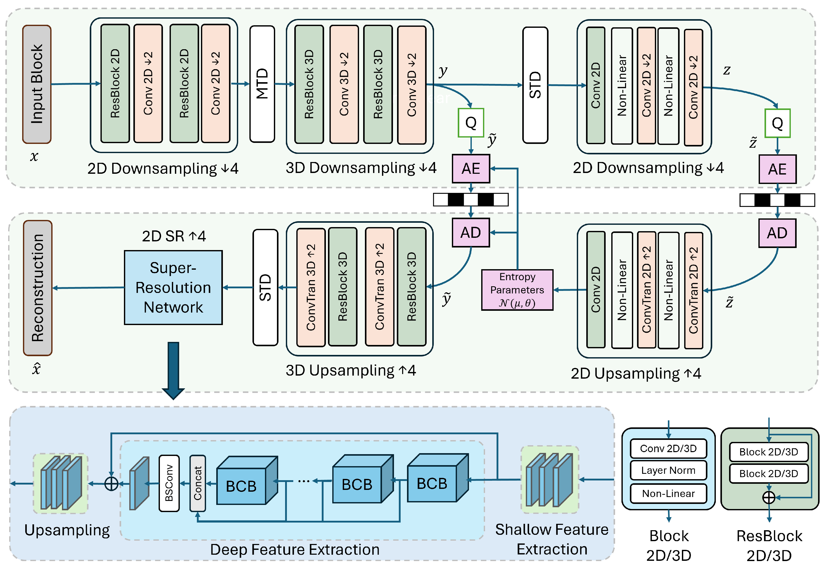
The transform-based Foundation Model (FM) consists of two main components, referred to as CAESAR-V: a VAE with a hyperprior structure and a super-resolution (SR) module. First, we extend the hyperprior-based VAE from 2D to 3D to effectively capture spatio-temporal correlations within the data. Then, a 2D SR module is applied to enhance the fidelity of each individual time slice. The details of these components are described below.

3.2.1. Variational 3D Autoencoder

We design a variational 3D autoencoder combining 2D and 3D convolutions to balance efficiency and representational capacity. Given input dimensions [ T , H , W ] , 2D convolutions and downsampling are first applied to each temporal slice, producing features of C , H 4 , W 4 . These are stacked along the temporal axis into C , T , H 4 , W 4 , followed by 3D convolutions and downsampling to obtain latent representations 2 C , T 4 , H 16 , W 16 , denoted as y .
After quantization, the decoder uses transposed 3D convolutions for upsampling, restoring dimensions to 2 C , T , H 4 , W 4 , and an SR module reconstructs the final output [ T , H , W ] . To model the quantized latent space y ˜ , we split the temporal dimension into T 4 slices. Each is compressed via a hyper-prior autoencoder, producing a hyper-latent representation z of size 4 C , H 64 , W 64 . The hyper-prior decoder predicts the mean and standard deviation for each latent slice.

3.2.2. SR Module

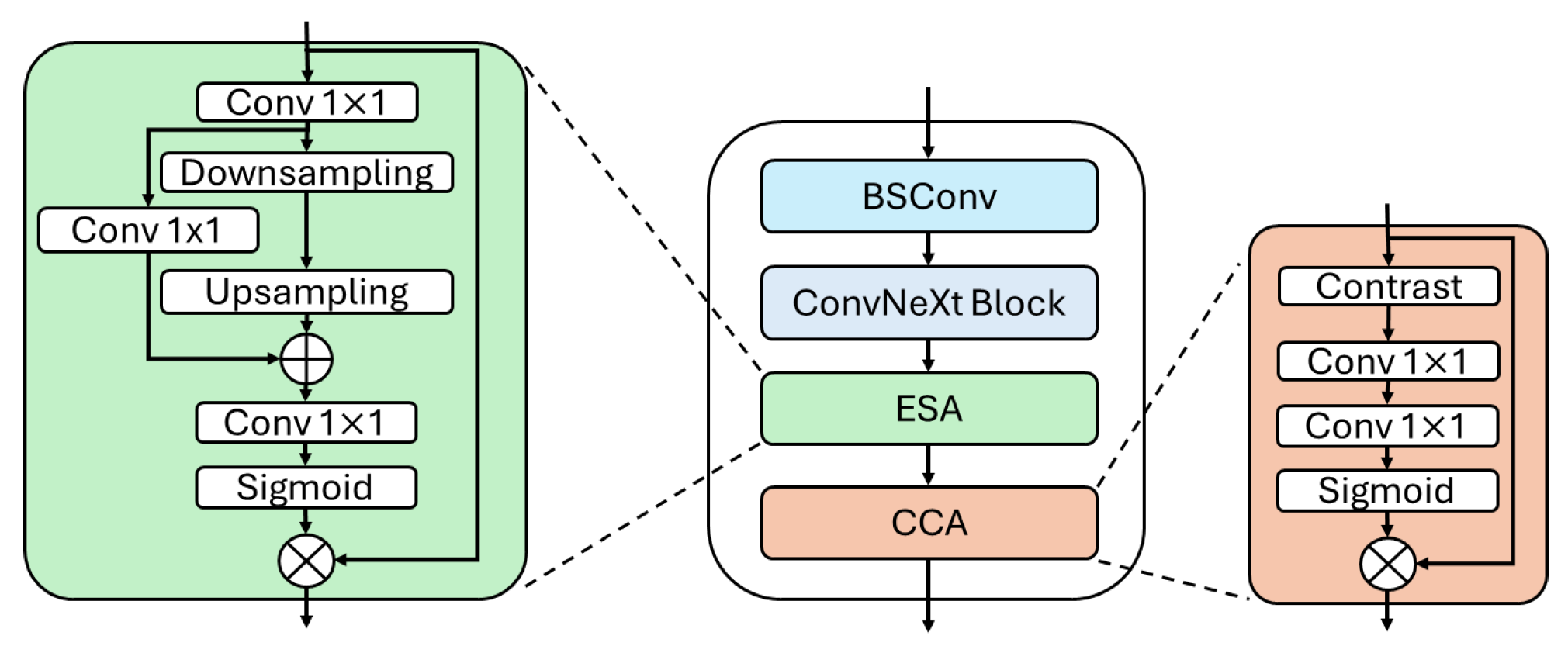
As decoding in lossy compression involves upsampling, we adopt a super-resolution (SR) architecture inspired by [30]. As illustrated in Figure 2, it starts with a shallow feature extractor, followed by multiple BCB blocks shown in Figure 3, each containing a BSConv layer [31], a ConvNeXt block [32], and two attention modules: ESA and CCA.
The ESA module reduces channel dimensions via a 1 × 1 convolution, downsamples with convolutions and max pooling, upsamples by interpolation, and applies a sigmoid attention mask. The CCA module [33] uses channel statistics (mean and standard deviation) to compute contrast-aware attention through 1 × 1 convolutions and a sigmoid activation.
As shown in Figure 2, outputs from all BCB blocks are concatenated, capturing multi-level features. A skip connection merges shallow and deep features to reinforce the reconstruction. Finally, a channel shuffle layer upsamples the spatial resolution by a factor of 4.

3.2.3. Compression and Decompression Procedure

During compression, each input data block is first passed through the pretrained variational autoencoder (VAE), which combines 2D and 3D convolutions to capture spatiotemporal features. The resulting latent tensor is quantized and split along the temporal axis into segments, each of which is further encoded using a hyperprior-based entropy model. The compressed bitstream consists of both the quantized latent codes and their corresponding hyper-latents.
For decompression, the latent codes are entropy-decoded using the predicted mean and scale parameters from the hyperprior decoder. The decoded latent representations are then passed through the VAE decoder and the super-resolution (SR) module to reconstruct the original data block.
All model parameters are pretrained offline and remain fixed during both compression and decompression. The total model size of CAESAR-V is approximately 5.9 MB. We report inference time only, excluding any training or fine-tuning procedures.

3.3. CAESAR-D Foundation Model

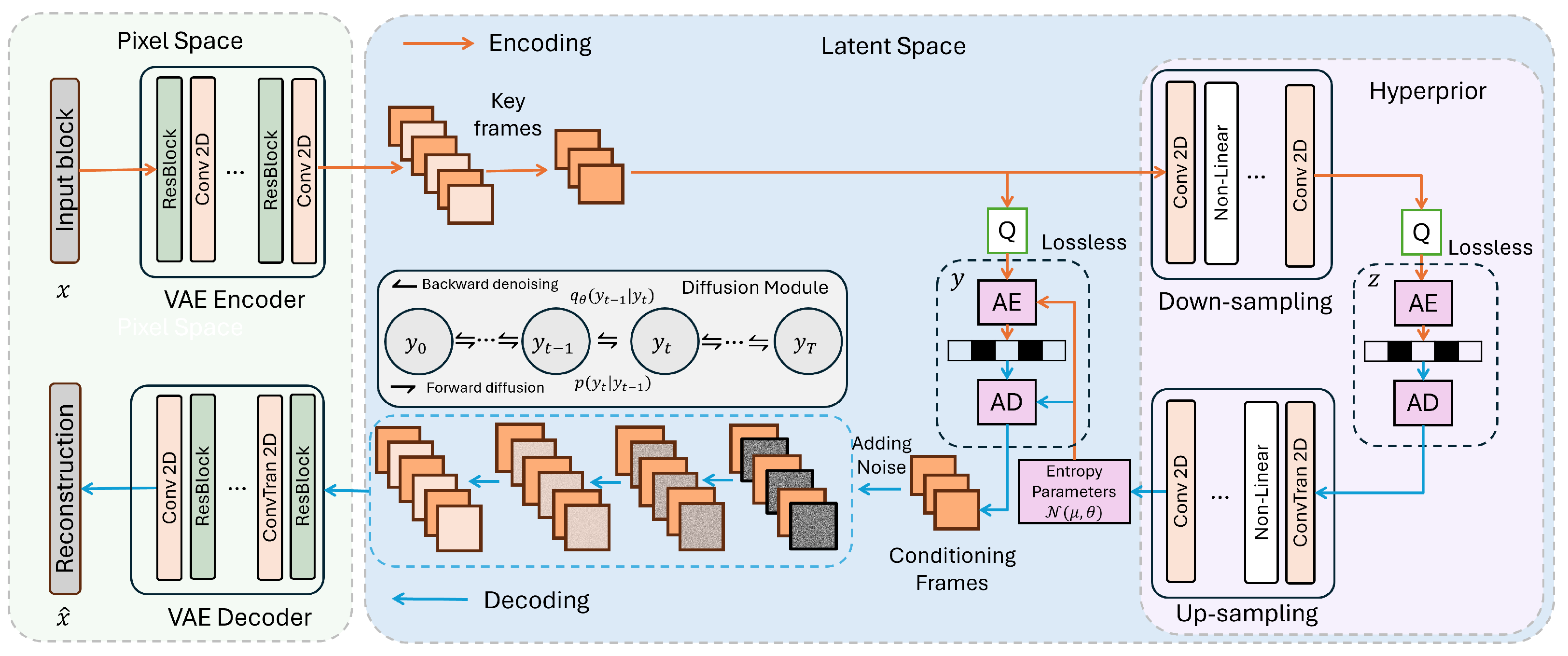
Conventional methods store latents for every frame, increasing storage overhead. To address this, we propose a generative strategy using latent diffusion, storing only keyframe latents and generating intermediate ones conditionally. Our CAESAR-D framework, shown in Figure 4, consists of a VAE with hyperpriors to compress keyframes and a latent diffusion model to generate missing latents from nearby keyframes. The decoder then reconstructs the full sequence from both stored and generated latents. Module details are provided in the following sections.

3.3.1. Latent Diffusion Models

Latent diffusion models [34,35] are generative frameworks that learn to recover clean latent data p ( y ) by progressively denoising Gaussian noise through a Markov chain with T steps. In the forward process, noise is added at each step:
q ( y t | y t 1 ) = N ( y t | 1 β t y t 1 , β t I ) ,
or directly in terms of the original latent:
q ( y t | y 0 ) = N ( y t | α ¯ t y 0 , ( 1 α ¯ t ) I ) ,
where α ¯ t = i = 1 t ( 1 β i ) . A neural network ϵ θ predicts the noise at each step, enabling the reverse denoising. The training objective is:
L DM = E y , ϵ , t ϵ ϵ θ ( y t , t ) 2 2 ,
with t randomly sampled. By iteratively denoising, the model generates realistic samples from pure noise.

3.3.2. Keyframe Conditioning

We adopt a conditional diffusion framework for latent representations, originally introduced in our earlier work [6], which employs a U-Net architecture [36] for denoising. Let y 0 N R N , C , W , H denote the quantized latent variables for a sequence of N frames, where C, W, and H represent the latent channels, width, and height, respectively. To maintain consistency with the diffusion noise schedule, we normalize the latent values to the range [ 1 , 1 ] using min-max scaling.
The latent sequence is partitioned along the temporal axis into two disjoint subsets: the frames to be synthesized y 0 G R N K , C , W , H and a set of conditioning frames y 0 C R K , C , W , H , such that G C = and G C = N . We express the full latent sequence as y 0 N = y 0 G y 0 C , where the concatenation operator ⊕ is defined as
( a G b C ) i : = a i , if i G , b i , if i C .
In contrast to existing approaches that integrate conditioning information via cross-attention mechanisms or auxiliary inputs to the denoising network [37,38], we directly supply both the noisy target frames and clean conditioning frames to the network ϵ θ . During the forward diffusion process, Gaussian noise is gradually added to the frames in y 0 G according to
y t G N α ¯ t y 0 G , ( 1 α ¯ t ) I .
At each denoising step, the noised target frames y t G are combined with the conditioning frames y 0 C to form y t N = y t G y 0 C . The network predicts the noise residual for the entire sequence, but the loss is computed only for the target frames:
L CDM = E y N , ϵ N ( 0 , 1 ) , t ϵ ϵ θ ( y t N , t ) G 2 2 ,
where ϵ has the same dimensions as y t G . This strategy simplifies conditioning while preserving temporal context throughout the denoising process.

3.3.3. Compression and Decompression Procedure

The CAESAR-D framework compresses only selected keyframes within a spatiotemporal sequence. Each keyframe is processed through a VAE encoder with similar structure to that of CAESAR-V, but trained separately as a keyframe compressor in CAESAR-D, which are then quantized and compressed via a hyperprior-based entropy model. Latents for non-keyframes are discarded during compression, resulting in significantly reduced storage requirements.
Decompression proceeds in three stages. First, the compressed keyframe latents are entropy-decoded. Second, a pretrained conditional latent diffusion model is used to reconstruct missing latent frames by iteratively denoising noisy inputs conditioned on nearby keyframe latents. Finally, the complete latent sequence, including both decoded and generated latents, is fed into the VAE decoder to reconstruct the full data block.
All components of CAESAR-D are pretrained and remain unchanged during deployment. The combined model size, including both the VAE and the diffusion model, is approximately 141 MB. As with CAESAR-V, runtime analysis includes only inference time.

3.4. Model Training

Both CAESAR-V and CAESAR-D use a Variational Autoencoder (VAE) with hyperprior for latent representation learning. CAESAR-V is trained end-to-end, while CAESAR-D follows a two-stage training approach from our previous work [6]. In the first stage, the VAE balances reconstruction accuracy and bitrate by minimizing
L = MSE ( x , x ^ ) + λ E y log 2 p ( y μ , σ ) + E z log 2 p ( z ) ,
where distortion is measured by the Mean Squared Error (MSE), and the rate terms correspond to the latent y and hyper-latent z representations.
Once the VAE converges, the encoder is frozen. In the second stage, a latent diffusion model is trained on the compressed latent representations to capture temporal dependencies and iteratively denoise noised latent frames conditioned on selected context frames. Full training procedures, including quantization strategies, forward diffusion formulation, and loss computation for the conditional diffusion model, are described in detail in [6].

3.5. Error Bound Guarantees and GPU Acceleration

3.5.1. PCA-Based Error Bound Guarantee

Maintaining a guaranteed error bound is critical in scientific data compression to preserve the fidelity of reconstructed data, particularly for large-scale, high-dimensional datasets. Building upon prior work [3,20,39,40], we implement a PCA-based approach to enforce this guarantee. After performing compression and decompression, we compute the residuals and apply Principal Component Analysis (PCA) to identify the dominant components, forming the basis matrix U . The residual is then projected onto this basis to calculate the coefficient vector c :
c = U T ( x x R ) .
To meet the prescribed error threshold τ , we select the top M coefficients whose cumulative contribution ensures that the residual’s 2 -norm satisfies x x G 2 τ . These coefficients are subsequently quantized and entropy encoded for efficient storage. The final corrected reconstruction is expressed as
x G = x R + U s c q ,
where c q denotes the quantized selected coefficients and U s represents their associated basis vectors.

3.5.2. Quantization Bin Upper Bound

We quantize the PCA coefficients c using a uniform quantization bin width b with a rounding operation, obtaining quantized coefficients c q . Typically, using a larger quantization bin reduces the number of unique quantized values and improves compression efficiency, but at the cost of increased reconstruction error. To determine the maximum allowable bin width while preserving a user-specified error tolerance, we derive an upper bound on b. After quantization, the reconstructed data is given by
x G = x R + U s c q ,
and the quantization error in the residual is
e = U s ( c c q ) .
Because the PCA basis vectors U s are orthonormal, the total 2 error is equal to the norm of the quantization errors in coefficient space:
e 2 = c c q 2 .
Since each coefficient incurs a maximum quantization error of b 2 , the worst-case total error is
e 2 b 2 M ,
where M is the dimensionality of c . To ensure this total error remains within a target error bound eb, we require
b 2 M eb .
Solving for b, we obtain the quantization bin upper bound:
b 2 eb M .

3.5.3. GPU Acceleration

The bottleneck limiting the speed of the post-processing stage is the selection of coefficients to retain for each instance. The key idea for GPU acceleration is to vectorize this selection process, enabling parallel processing of all instances simultaneously. Traditionally, this involves sequentially calculating the 2 norm x x R 2 after adding each coefficient to determine the stopping criterion—a procedure with a computational complexity of O ( M 2 ) due to repeated reconstruction and error measurement.
To address this, we leverage the orthogonality of the PCA basis vectors, which allows the reconstruction error to be computed directly from the coefficients without explicit reconstruction. Specifically, when selecting the top k coefficients, the reconstruction error simplifies to
e k 2 2 = i = 1 k ( c i c q , i ) 2 + i = k + 1 M c i 2 ,
where e k denotes the reconstruction error after retaining the top k quantized coefficients. The first term of the right side represents the quantization error on these k coefficients, while the second term accounts for the residual energy of the remaining, unselected coefficients. To facilitate parallel computation, we maintain a list L for each instance that records the cumulative error after adding each coefficient L [ k ] = e k 2 2 . We further observe that the incremental change in error when
L [ k + 1 ] L [ k ] = ( c k + 1 c q , k + 1 ) 2 c k + 1 2 .
This allows L to be updated incrementally with O ( 1 ) complexity per element, and O ( M ) per instance—operations that are trivially parallelizable on GPUs. We compute each L [ k ] across all instances in a batched, vectorized fashion on the GPU. Finally, to determine the number of coefficients to retain for each instance, we perform a parallel search for the index of the first element in each L that meets the target error bound, fully leveraging GPU parallelism throughout the post-processing stage.

4. Experiments

In this section, we first describe the evaluation metrics and datasets used in our experiments. We then examine different conditioning strategies to identify which yields the best compression performance. After that, we detail the hyperparameters selected for our experiments. We proceed to compare our approach with current leading methods based on compression ratio and error trends. Lastly, we assess the computational efficiency of our method in comparison to other state-of-the-art techniques.

4.1. Evaluation Metrics and Datasets

We use Normalized Root Mean Square Error (NRMSE) to measure reconstruction quality relative to the data range, accommodating datasets with different scales. The NRMSE is defined as
NRMSE ( Ω , Ω ^ G ) = Ω Ω ^ G 2 / N d max ( Ω ) min ( Ω ) ,
where N d is the total number of data points, Ω is the original dataset, we use a suitable norm · (related to the 2 norm for vectors), and Ω ^ G is the reconstructed dataset after error-bound post-processing.
Table 1 summarizes the datasets used in our experiments, including their application domains, dimensions, and total sizes. Detailed descriptions of each dataset are provided below:
  • E3SM Dataset
The Energy Exascale Earth System Model (E3SM) [7] simulates Earth’s climate at high resolution. We use hourly atmospheric data on a 25 km grid ( 0 . 25 ), producing about 350,000 points per variable. A Cube-to-Sphere projection maps the data to a flat grid, yielding a dataset of size 5 × 6 × 9360 × 240 × 240 (variables, regions, time steps, and spatial resolution).
  • S3D Dataset
The S3D dataset models the compression ignition of fuel-lean n-heptane/air mixtures under HCCI-relevant conditions [8]. It captures 58 chemical species over 50 time steps on a 640 × 640 grid, forming tensors of size 58 × 50 × 640 × 640 .
  • JHTDB Dataset
From the Johns Hopkins Turbulence Database (JHTDB) [9], we use isotropic turbulence simulation data with 3D velocity fields on a Cartesian grid. Our subset includes 64 spatial regions over 256 time steps, each frame sized 512 × 512 , resulting in a dataset of shape 64 × 256 × 512 × 512 .
  • ERA5 Dataset
The ERA5 dataset is a global atmospheric reanalysis product provided by the European Centre for Medium-Range Weather Forecasts (ECMWF) [41], offering hourly estimates of a large number of atmospheric, land, and oceanic climate variables. For our experiments, we utilize a subset of ERA5, resampled and preprocessed into a regular spatiotemporal grid suitable for learning-based models. The data is stored in float32 precision and includes six key climate variables: Geopotential, Ozone mass mixing ratio, Specific humidity, Temperature, V-component of wind, and Vertical velocity. The resulting tensor has the shape 6 × 3 × 2160 × 512 × 512 , where 6 is the number of variables, 3 represents vertical levels, 2160 indicates the number of time steps, and each frame has a spatial resolution of 512 × 512 .
  • Hurricane Dataset
We utilize a subset of the Hurricane dataset from [42], a widely used resource for simulating and analyzing the structure and evolution of tropical cyclones. The full dataset captures multiple meteorological variables over a structured three-dimensional grid with a spatial resolution of 500 × 500 and 100 vertical levels across 48 time steps. In this study, we focus on three key variables: pressure, temperature, and windspeed along the Z-axis. To balance computational efficiency and maintain essential dynamic behavior, we extract a subset comprising 32 vertical levels and 47 temporal frames. This selection retains the critical physical structures necessary for evaluating data compression and reconstruction performance in extreme weather simulations.
  • TUM-TF Dataset
We use the TUM-TF dataset from the Technical University of Munich [43], which provides velocity field data from direct numerical simulations of turbulent flow within complex domains. The original data is stored in unstructured meshes. To convert it into a structured format suitable for learning, we extract 16 equally spaced 2D slices along the x-axis from the 3D field, each with a thickness of 0.002 and interpolated onto a 256 × 256 grid in the y z -plane. This slicing process is performed across 2000 time steps, resulting in a tensor of shape 3 × 16 × 2000 × 256 × 256 , where 3 denotes the velocity components ( v x , v y , v z ). All values are stored as float32.
  • HYCOM Dataset
The HYCOM dataset [44] is derived from the Hybrid Coordinate Ocean Model, which provides high-resolution simulations of global ocean dynamics. In our experiments, we use a preprocessed subset of HYCOM data containing four physical variables: water_u, water_v, water_temp, and salinity. The dataset has been formatted into regular grids and stored in float32 precision. To construct the final tensor, we select 4 valid spatial ocean blocks with consistent coverage and extract 16 vertical depth layers from each, resulting in 64 spatial channels. The resulting tensor has shape 4 × 64 × 128 × 256 × 256 , where 4 denotes the number of variables, 64 the number of depth-based channels, 128 the number of time steps, and each frame has a spatial resolution of 256 × 256 .
  • PDEBench Dataset
The PDEBench dataset [45] provides simulation data for a variety of canonical partial differential equations (PDEs), including advection, Burgers’, diffusion-reaction, diffusion-sorption, shallow water, Darcy flow, and compressible Navier-Stokes equations in 1D to 3D. In our study, we utilize a 2D incompressible Navier-Stokes subset from the dataset with shape 3 × 16 × 128 × 512 × 512 , where 16 represents the number of simulation blocks, 128 is the number of time steps, and 3 denotes the three fields used: velocity components v x , v y , and particle concentration. All values are stored in float32 precision.
  • OpenFOAM Dataset
We construct a synthetic fluid dynamics dataset using the OpenFOAM toolbox [46], a widely used open-source CFD solver. The initial velocity fields are generated by placing multiple Gaussian vortices with varying strengths and locations. These serve as initial conditions for incompressible Navier-Stokes simulations under periodic boundary conditions. The resulting dataset has the shape 3 × 4 × 1200 × 512 × 512 , where 3 represents the physical variables vx, vy, and p; 4 denotes different vortex configurations; 1200 is the number of simulated time steps; and each frame has a spatial resolution of 512 × 512 . All values are stored in float32 precision.
Table 1. Datasets Information.
ApplicationDomainDimensionsTotal Size
E3SMClimate 5 × 6 × 9360 × 240 × 240 61 GB
S3DCombustion 58 × 1 × 50 × 640 × 640 8.9 GB
JHTDBFluid Dynamics 3 × 64 × 256 × 512 × 512 45 GB
ERA5Atmospheric Reanalysis 6 × 3 × 2160 × 512 × 512 21 GB
HurricaneWeather 3 × 32 × 47 × 500 × 500 4.3 GB
TUM-TFTurbulence 3 × 16 × 2000 × 256 × 256 19 GB
HYCOMOceanology 4 × 64 × 128 × 256 × 256 3.6 GB
PDEBenchPhysics 3 × 16 × 128 × 512 × 512 5.6 GB
OpenFOAMCFD 3 × 4 × 1200 × 512 × 512 15 GB

4.2. Implementation Details

Model training was performed on the HiPerGator Supercomputer using a single NVIDIA A100 GPU per model with PyTorch 2.2.0. Training has two phases: first the VAE with hyperprior, then the latent diffusion model.
For the VAE, 256 × 256 patches are randomly cropped with a batch size of 32. Smaller datasets (e.g., E3SM) use reflection padding. The learning rate starts at 1 × 10 3 and halves every 100,000 iterations; λ starts at 1 × 10 5 and doubles at 250,000 iterations, with training continuing for 500,000 iterations total. Each frame is normalized to zero mean and unit range due to large data value ranges. These settings apply to both CAESAR-V and the keyframe compressor in CAESAR-D. The latent diffusion model trains with 1000 denoising steps for 500,000 iterations, then fine-tunes with 32 steps for 200,000 iterations. Batch size is 64, learning rate 1 × 10 4 , sequence length 16, and 64 latent channels. Mean squared error (MSE) loss is used.
Testing is performed on E3SM, S3D, and JHTDB datasets; all other data is reserved for training. Foundation models CAESAR-V and CAESAR-D are trained on the training data, then fine-tuned per domain. CAESAR-V fine-tunes for 100,000 iterations at a learning rate of 1 × 10 4 . CAESAR-D fine-tunes the keyframe compressor for 100,000 iterations and the latent diffusion model for 200,000 iterations at the same rate.

4.3. Keyframe Selection

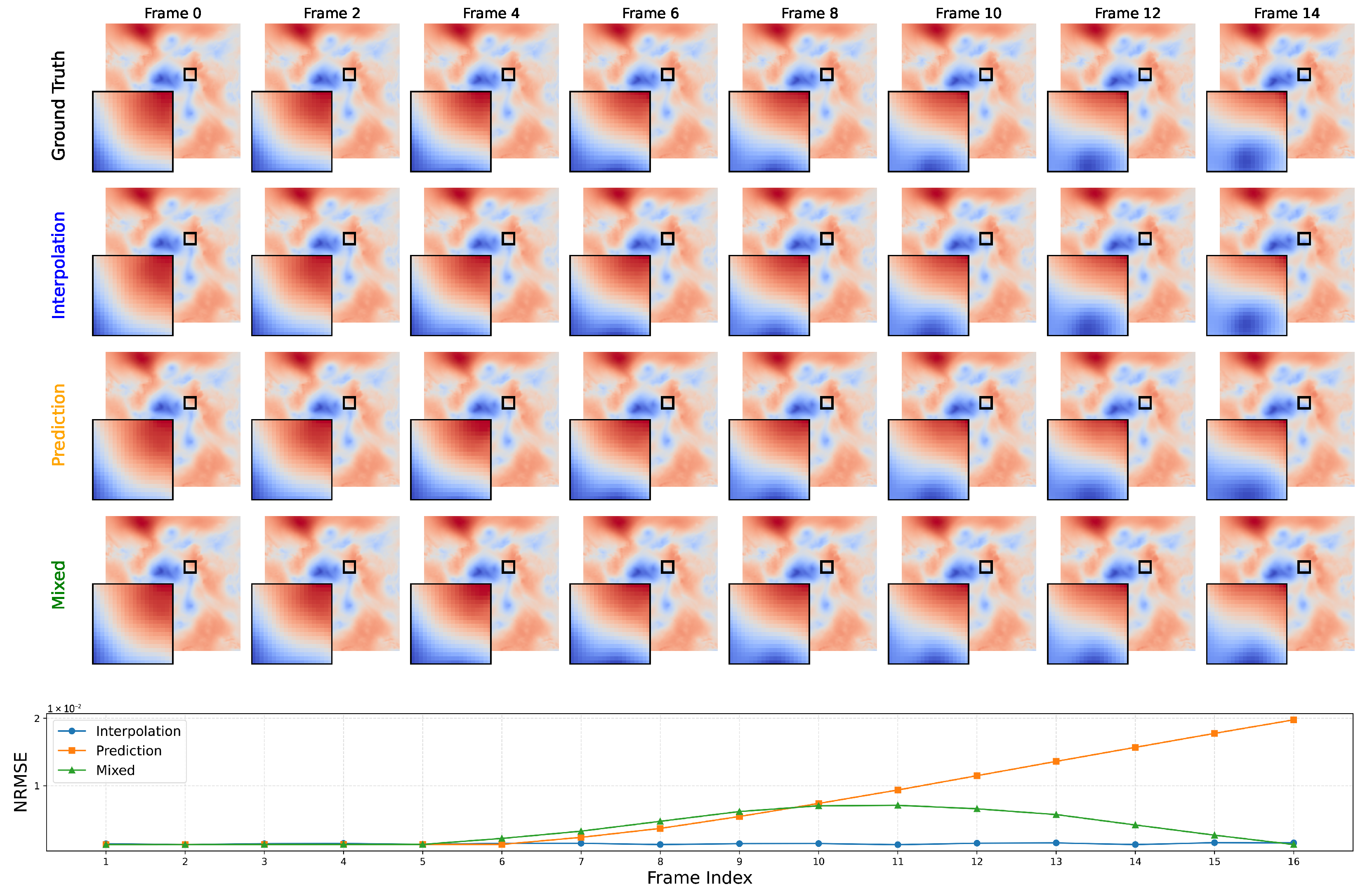
For the CAESAR-D model, we explore three different strategies for selecting keyframes: prediction-based, interpolation-based, and a mixed approach. In the prediction-based strategy, the initial 6 frames are designated as conditioning frames, and the remaining frames are sequentially predicted based on temporal dependencies. The interpolation-based strategy selects 6 keyframes uniformly across the sequence, allowing the model to interpolate intermediate frames conditioned on these evenly distributed reference points. The mixed strategy combines both by selecting the first 6 frames and the final frame, providing early and late temporal context.
Figure 5 presents qualitative visualizations of the original and reconstructed data, along with frame-wise reconstruction errors for each strategy. Among the three, the interpolation-based strategy consistently achieves the lowest reconstruction error, benefiting from evenly spaced keyframes that reduce large temporal gaps. Across all approaches, reconstruction error decreases for frames closer to the conditioning frames, highlighting the importance of keyframe distribution in maintaining temporal consistency and reconstruction accuracy.

4.4. Impact of Keyframe Interval and Denoising Steps

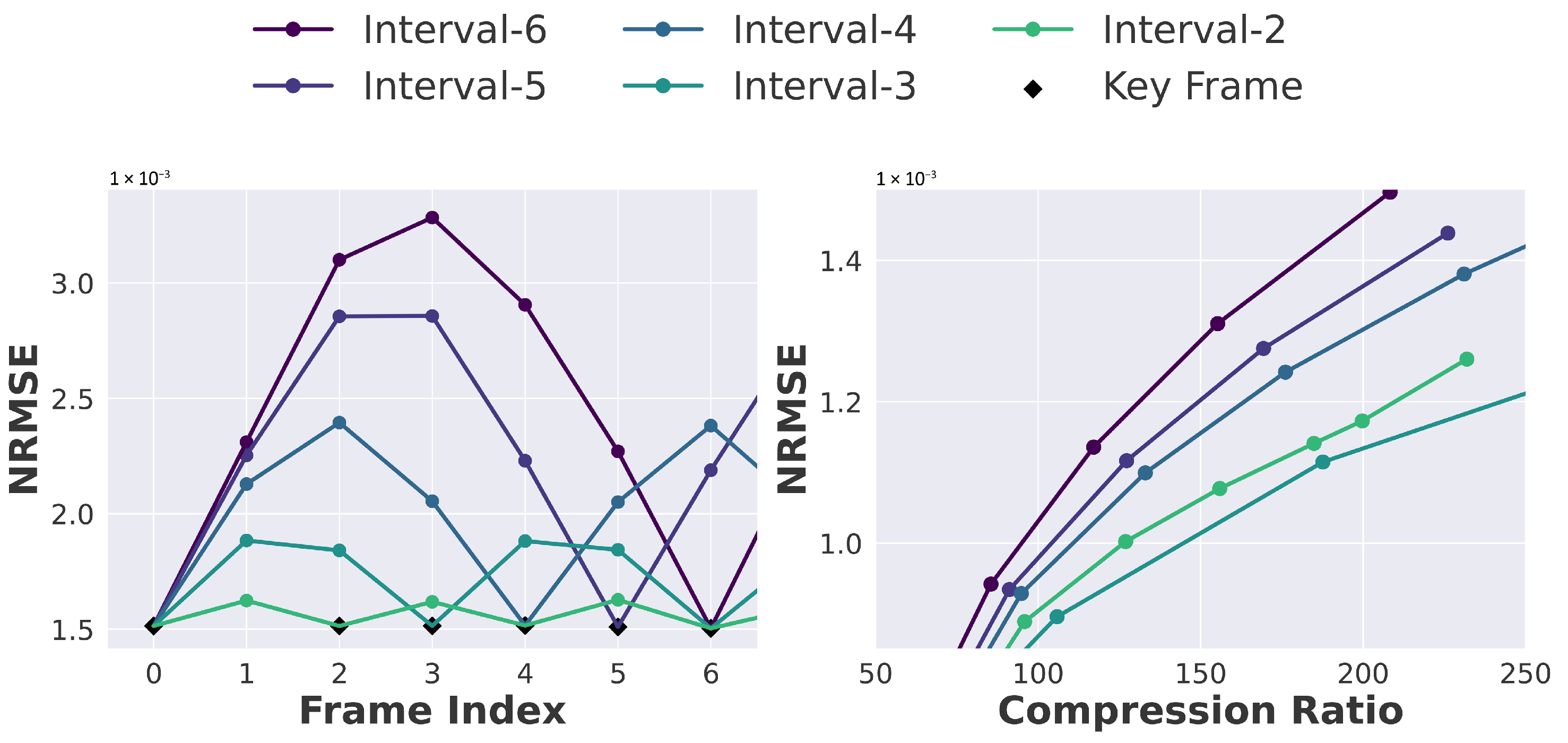
Increasing the keyframe interval in interpolation-based compression can substantially improve compression ratios, as fewer keyframes need to be stored or transmitted. However, this advantage often comes at the cost of increased reconstruction errors, since the model must infer a greater number of intermediate frames without direct reference data. To investigate this trade-off, we conducted experiments on the E3SM dataset using keyframe intervals ranging from 2 to 6 (Figure 6). The results show that smaller intervals consistently yield lower normalized root mean square error (NRMSE) values, benefiting from more frequent conditioning on actual keyframes. Conversely, larger intervals lead to higher errors due to the increased reliance on interpolation. Notably, an interval of 3 achieves the most favorable balance between compression efficiency and reconstruction accuracy, offering substantial storage savings without a significant loss in fidelity. Similar trends are observed across other datasets, though the optimal choice of keyframe interval is inherently data-dependent, influenced by the temporal dynamics and smoothness of the underlying scientific data.
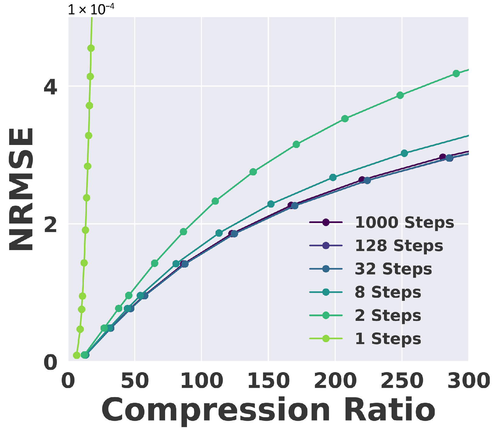
Diffusion model quality depends on the number of denoising steps, which affects generation speed. Using a two-phase training strategy—initial training with 1000 steps followed by fine-tuning with fewer steps—allows maintaining accuracy with as few as 32 steps (Figure 7), significantly speeding up inference without degrading compression performance.

4.5. Comparison with Other Methods

We evaluate our method on three benchmark datasets and compare it against two state-of-the-art scientific data compressors: SZ3 [5] and ZFP [47]. SZ3 employs a prediction-based approach, while ZFP uses transform-based compression. We report the performance of our foundation models trained on the full training set without domain-specific fine-tuning, as well as the performance after fine-tuning for both CAESAR-V and CAESAR-D. We denote the foundation model performance as ‘FM’ and the fine-tuned model performance as ‘FMFT’.
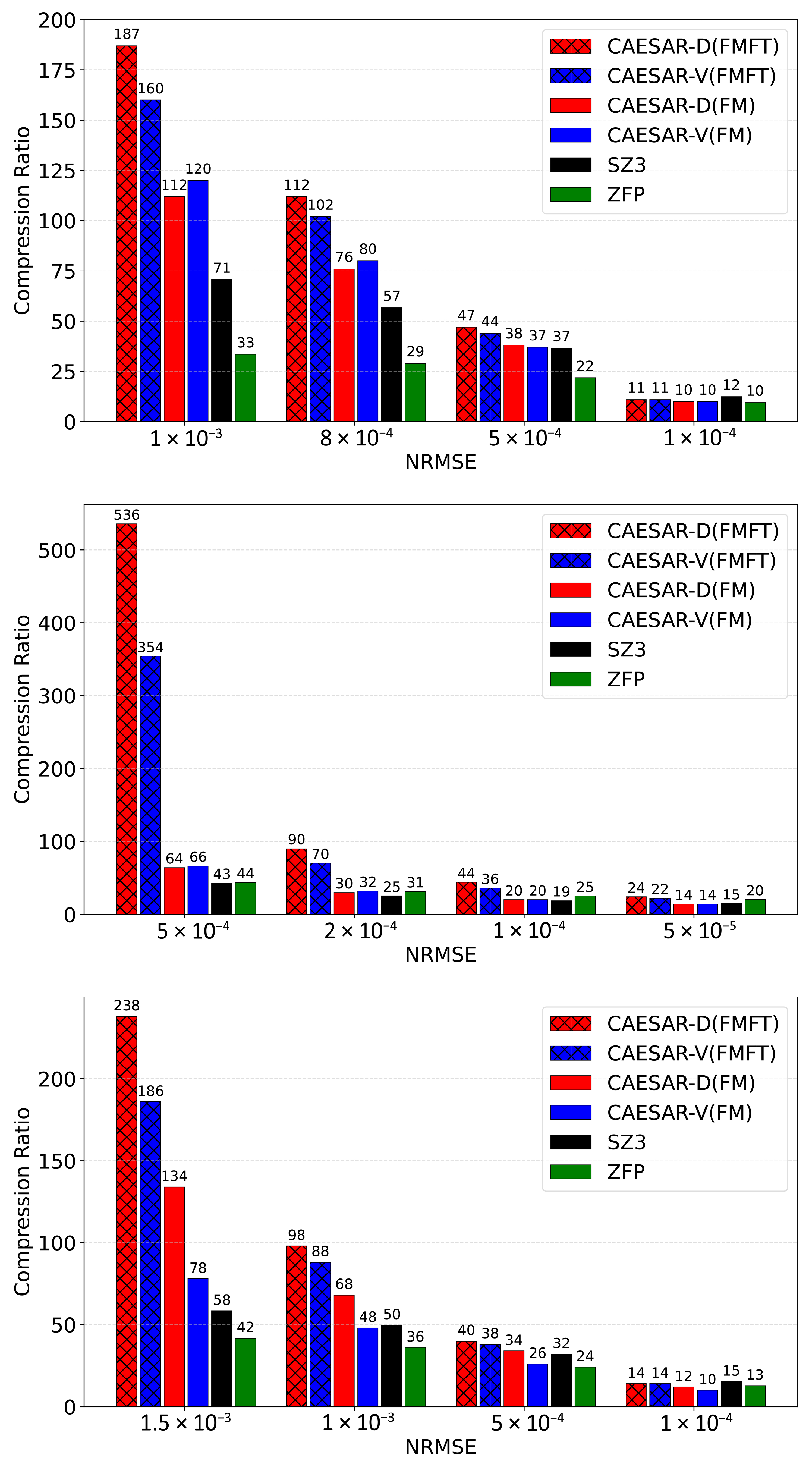
As shown in Figure 8, our method achieves substantial compression improvements across all three datasets compared to ZFP and SZ3. In the figure, methods based on the same model architecture are indicated with the same color for clarity. Overall, both our foundation models and their domain-specific fine-tuned versions consistently outperform SZ3 and ZFP. Notably, CAESAR-D achieves performance comparable to CAESAR-V under foundation training and surpasses it after domain-specific fine-tuning. Fine-tuning consistently improves the compression ratio at the same reconstruction error, with gains ranging from 1.5× to 10× across different datasets.
Specifically, CAESAR-V (FM) and CAESAR-D (FM) outperform SZ3 by over 2× in compression ratio, and after domain-specific fine-tuning, our methods achieve more than 3× improvement on the E3SM dataset. We also observe significant fine-tuning gains on the S3D dataset, highlighting the importance of domain adaptation for scientific data. On S3D, CAESAR-D surpasses SZ3 by over 10× after fine-tuning. Both CAESAR-V and CAESAR-D improve by roughly 8× with domain-specific fine-tuning compared to FM training. For the JHTDB dataset, CAESAR-D outperforms CAESAR-V by a factor of 2 under foundation training. After domain-specific fine-tuning, both models achieve more than 3× higher compression ratios compared to SZ3. To facilitate comparison, we also present the results in Figure 9, which shows the compression ratios achieved at specific error bounds in term of NRMSE. Notably, while CAESAR maintains a substantial advantage under moderate error bounds (e.g., NRMSE ≥ 5 × 10 4 ), its compression ratio decreases as the target error becomes more stringent. At very low error thresholds (e.g., NRMSE ≤ 1 × 10 4 ), the observed advantage over SZ3 and ZFP narrows, and the performance of CAESAR becomes comparable to traditional compressors. This effect arises from the PCA-based postprocessing module, which is activated to enforce strict error guarantees on reconstructed data. While this step is critical for maintaining numerical fidelity, it introduces additional bit cost due to the inclusion of correction information, thereby reducing the final compression ratio. This trade-off is an intentional design choice, prioritizing accuracy over compression efficiency when operating under tight error constraints.
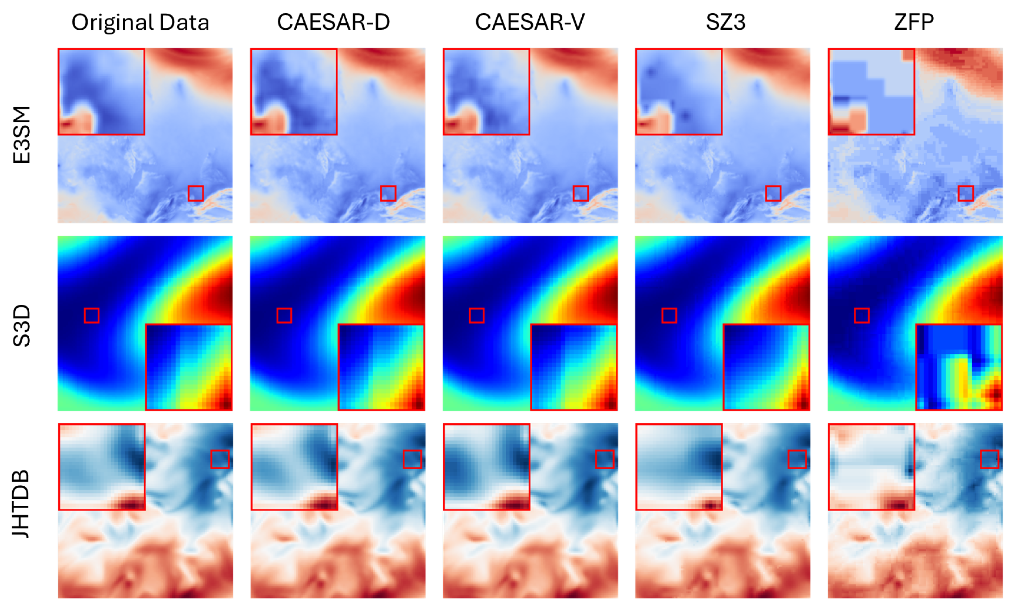
Figure 10 presents reconstructed fields from CAESAR-D, CAESAR-V, SZ3, and ZFP on three representative datasets (E3SM, S3D, and JHTDB) at a compression ratio of approximately 100, with the original data provided for reference. Each case includes two red rectangles: one marking a region of interest in the full frame, and the other presenting a zoomed-in view for detailed inspection. Across all datasets, CAESAR-D demonstrates the most faithful reconstruction, preserving fine-scale structures, smooth gradients, and coherent spatial patterns with minimal artifacts, closely matching the ground truth. CAESAR-V achieves similar performance but exhibits slight attenuation of high-frequency details, while SZ3 produces noticeable blurring and occasional ringing effects near sharp transitions. ZFP, although competitive in smooth regions, introduces pronounced block artifacts and visible distortions in areas of complex variation. These qualitative observations are consistent with the quantitative metrics reported earlier, reinforcing that CAESAR-D not only maintains superior visual fidelity at high compression ratios but also provides more stable reconstruction quality across diverse scientific data domains.
To further validate the reliability of CAESAR in scientific data compression, we analyze the vector-wise reconstruction accuracy of CAESAR-D. While global metrics such as average NRMSE provide a general sense of model performance, scientific applications often require spatially consistent accuracy across the entire domain.
We compress the E3SM dataset using a global absolute error bound of 1 × 10 3 . The data is divided into 3.89 million non-overlapping 1 × 64 vectors. For each vector, we compute the NRMSE after decompression and present the histogram of these values in Figure 11. The compression ratio achieved under this setting is 158.5 and the red dashed line indicates the overall dataset-level NRMSE of 7.31 × 10 4 .
This analysis shows the model’s ability to maintain uniform reconstruction quality across space. In contrast to traditional compressors that may over-compress certain regions and under-compress others, CAESAR offers more stable and predictable error behavior. Such consistency is particularly important in scientific applications where localized errors can significantly impact downstream simulations or analyses.

4.6. Model Inference Speed

To evaluate the inference efficiency of our proposed models, we benchmarked the performance of both CAESAR-V and CAESAR-D on two different hardware configurations: an NVIDIA A100 80 GB GPU and an NVIDIA RTX 2080 24 GB GPU. We report encoding and decoding speeds separately to provide a detailed breakdown of computational cost and assess scalability across devices.
Both CAESAR-V and CAESAR-D share a common architectural principle: the encoder is designed to be lightweight and efficient, while the decoder handles most of the computational workload. For CAESAR-V, both encoding and decoding involve direct transform-based operations, resulting in balanced and consistently high throughput on both GPUs. CAESAR-D, in contrast, adopts a two-stage strategy where keyframes are compressed by a VAE-based encoder while non-key frames are reconstructed through a diffusion process during decoding. As a result, CAESAR-D achieves higher encoding speeds, since only keyframes require compression, but its decoding speed is influenced by the number of diffusion steps used. Notably, reducing the number of diffusion steps from 128 to 8 leads to substantial improvements in decoding throughput, with minimal degradation in reconstruction quality as demonstrated in our quantitative evaluations.
Table 2 summarizes the inference speeds in megabytes per second (MB/s) for both models and devices. On the A100 GPU, CAESAR-V achieves 943 MB/s encoding and 652 MB/s decoding speeds, while CAESAR-D reaches up to 1942 MB/s for encoding and 203 MB/s decoding with 8 diffusion steps. Similar trends hold on the RTX 2080 GPU, with expected reductions in absolute throughput due to hardware limitations.

4.7. Post-Processing Speed on GPU

To evaluate the post-processing speed for enforcing error-bound guarantees on GPU, we use the reconstructed data generated by our diffusion model after domain-specific fine-tuning as a representative example. We test multiple error bounds in terms of the final NRMSE between the original data and the reconstructed data after post-processing. Typically, smaller error bounds require more computation time as more coefficients need to be processed and retained. Table 3 reports the compression speeds (in MB/s), and the relative speedup of the A100 over RTX 2080 GPUs under various NRMSE error bounds. After GPU acceleration, the post-processing step achieves real-time performance in compression workflows, enabling efficient integration into high-performance data compression pipelines.
In addition to GPU performance, we also report CPU-based compression speed as a reference. As shown in the table, CPU performance is significantly lower—over one to two orders of magnitude slower than GPUs. This result confirms that GPU acceleration is essential for integrating post-processing into practical, high-throughput compression workflows.

5. Limitations

While CAESAR demonstrates strong compression performance across various scientific datasets, some limitations remain.
First, as with any lossy compression framework, CAESAR introduces bounded approximation errors during reconstruction. Although we provide rigorous guarantees (e.g., NRMSE 10 3 ), users must assess whether the specified error bounds are acceptable for their specific downstream analyses. As discussed in Section 4.5, when extremely small error bounds (e.g., ≤10 4 ) are required, CAESAR’s compression advantage over traditional methods may diminish due to increased correction overhead. To achieve the intended high compression ratios, it is essential to select error bounds that align with the acceptable accuracy threshold of the application.
Second, our current evaluations are limited to fluid dynamics and climate datasets. Extending CAESAR to other scientific domains requires further investigation to ensure generalizability and effectiveness. In particular, domain adaptation to medical data may face challenges due to differences in data distribution, modality, and task objectives.
Lastly, CAESAR operates under the assumption of full data availability during compression. Adapting the framework to streaming or online encoding scenarios may require additional system-level development. In addition, training CAESAR involves moderate computational cost due to its use of deep generative models and multi-stage architectures. However, this cost is in line with other modern machine learning frameworks and is a one-time investment—once trained, CAESAR supports efficient, low-latency deployment.
We leave these directions for future work and emphasize the importance of aligning compression settings with domain-specific requirements to maximize the utility of learned compressors.

6. Conclusions

In this work, we introduced two complementary foundation model frameworks, CAESAR-V and CAESAR-D, for scalable, high-fidelity scientific data compression. By leveraging the principles of transfer learning and generalizable latent representations, both models demonstrate substantial improvements over traditional and contemporary compression techniques. The transform-based CAESAR-V offers efficient, fast encoding and decoding while preserving fine-grained spatiotemporal structures, whereas the generative CAESAR-D achieves superior compression ratios through learned temporal interpolation, albeit with higher computational cost.
Pretraining on diverse multi-domain scientific datasets enables both models to generalize effectively across applications, achieving over 2× higher compression ratios than state-of-the-art rule-based methods without domain-specific tuning. Further fine-tuning on target datasets yields an additional 1.5–5× compression improvement, all while upholding strict user-defined reconstruction error guarantees. The integration of a GPU-parallelized post-processing module ensures practical deployment in HPC workflows, supporting throughput of 0.4 1.1 GB/s.
Our results highlight the potential of foundation models for addressing the growing storage and transmission challenges in scientific computing. This work lays the groundwork for future research in data-driven, error-bounded, learned, scientific data reduction, opening pathways for adaptive, efficient, and scalable compression in next-generation HPC systems.

Author Contributions

Supervision, S.K., S.R. and A.R.; methodology, X.L., L.Z., J.L. and R.S. All authors have read and agreed to the published version of the manuscript.

Funding

This research was funded by the U.S. Department of Energy under Grant Nos. DE-SC0021320 and DE-SC0022265.

Conflicts of Interest

The authors declare no conflicts of interest.

References

  1. Kirillov, A.; Mintun, E.; Ravi, N.; Mao, H.; Rolland, C.; Gustafson, L.; Xiao, T.; Whitehead, S.; Berg, A.C.; Lo, W.Y.; et al. Segment anything. In Proceedings of the IEEE/CVF International Conference on Computer Vision, Paris, France, 2–3 October 2023; pp. 4015–4026. [Google Scholar] [CrossRef]
  2. Ainsworth, M.; Tugluk, O.; Whitney, B.; Klasky, S. Multilevel techniques for compression and reduction of scientific data-the univariate case. Comput. Vis. Sci. 2018, 19, 65–76. [Google Scholar] [CrossRef]
  3. Li, X.; Gong, Q.; Lee, J.; Klasky, S.; Rangarajan, A.; Ranka, S. Machine Learning Techniques for Data Reduction of Climate Applications. arXiv 2024, arXiv:2405.00879. [Google Scholar] [CrossRef]
  4. Li, X.; Lee, J.; Rangarajan, A.; Ranka, S. Attention based machine learning methods for data reduction with guaranteed error bounds. In Proceedings of the 2024 IEEE International Conference on Big Data (BigData), Washington DC, USA, 15–18 December 2024; IEEE: New York, NY, USA, 2024; pp. 1039–1048. [Google Scholar] [CrossRef]
  5. Liang, X.; Zhao, K.; Di, S.; Li, S.; Underwood, R.; Gok, A.M.; Tian, J.; Deng, J.; Calhoun, J.C.; Tao, D.; et al. SZ3: A modular framework for composing prediction-based error-bounded lossy compressors. IEEE Trans. Big Data 2022, 9, 485–498. [Google Scholar] [CrossRef]
  6. Li, X.; Zhu, L.; Rangarajan, A.; Ranka, S. Generative Latent Diffusion for Efficient Spatiotemporal Data Reduction. arXiv 2025, arXiv:2507.02129. [Google Scholar] [CrossRef]
  7. Golaz, J.C.; Caldwell, P.M.; Van Roekel, L.P.; Petersen, M.R.; Tang, Q.; Wolfe, J.D.; Abeshu, G.; Anantharaj, V.; Asay-Davis, X.S.; Bader, D.C.; et al. The DOE E3SM coupled model version 1: Overview and evaluation at standard resolution. J. Adv. Model. Earth Syst. 2019, 11, 2089–2129. [Google Scholar] [CrossRef]
  8. Yoo, C.S.; Lu, T.; Chen, J.H.; Law, C.K. Direct numerical simulations of ignition of a lean n-heptane/air mixture with temperature inhomogeneities at constant volume: Parametric study. Combust. Flame 2011, 158, 1727–1741. [Google Scholar] [CrossRef]
  9. Wan, M.; Chen, S.; Eyink, G.; Meneveau, C.; Perlman, E.; Burns, R.; Li, Y.; Szalay, A.; Hamilton, S. A public turbulence database cluster and applications to study Lagrangian evolution of velocity increments in turbulence. J. Turbul. 2008, 9, N31. [Google Scholar] [CrossRef]
  10. Fox, A.; Diffenderfer, J.; Hittinger, J.; Sanders, G.; Lindstrom, P. Stability analysis of inline ZFP compression for floating-point data in iterative methods. SIAM J. Sci. Comput. 2020, 42, A2701–A2730. [Google Scholar] [CrossRef]
  11. Ballester-Ripoll, R.; Lindstrom, P.; Pajarola, R. TTHRESH: Tensor compression for multidimensional visual data. IEEE Trans. Vis. Comput. Graph. 2019, 26, 2891–2903. [Google Scholar] [CrossRef]
  12. Ainsworth, M.; Tugluk, O.; Whitney, B.; Klasky, S. Multilevel techniques for compression and reduction of scientific data—The multivariate case. SIAM J. Sci. Comput. 2019, 41, A1278–A1303. [Google Scholar] [CrossRef]
  13. Gong, Q.; Chen, J.; Whitney, B.; Liang, X.; Reshniak, V.; Banerjee, T.; Lee, J.; Rangarajan, A.; Wan, L.; Vidal, N.; et al. MGARD: A multigrid framework for high-performance, error-controlled data compression and refactoring. SoftwareX 2023, 24, 101590. [Google Scholar] [CrossRef]
  14. Mun, S.; Fowler, J.E. DPCM for quantized block-based compressed sensing of images. In Proceedings of the 2012 Proceedings of the 20th European Signal Processing Conference (EUSIPCO), Bucharest, Romania, 27–31 August 2012; IEEE: New York, NY, USA, 2012; pp. 1424–1428. [Google Scholar] [CrossRef]
  15. Boyce, J.M.; Doré, R.; Dziembowski, A.; Fleureau, J.; Jung, J.; Kroon, B.; Salahieh, B.; Vadakital, V.K.M.; Yu, L. MPEG immersive video coding standard. Proc. IEEE 2021, 109, 1521–1536. [Google Scholar] [CrossRef]
  16. Liang, X.; Di, S.; Tao, D.; Li, S.; Li, S.; Guo, H.; Chen, Z.; Cappello, F. Error-controlled lossy compression optimized for high compression ratios of scientific datasets. In Proceedings of the 2018 IEEE International Conference on Big Data (Big Data), Seattle, WA, USA, 10–13 December 2018; pp. 438–447. [Google Scholar] [CrossRef]
  17. Liu, J.; Di, S.; Zhao, K.; Liang, X.; Chen, Z.; Cappello, F. FAZ: A flexible auto-tuned modular error-bounded compression framework for scientific data. In Proceedings of the 37th International Conference on Supercomputing, Orlando, FL, USA, 21–23 June 2023; pp. 1–13. [Google Scholar] [CrossRef]
  18. Kingma, D.P.; Welling, M. Auto-encoding variational Bayes. arXiv 2013, arXiv:1312.6114. [Google Scholar] [CrossRef]
  19. Minnen, D.; Ballé, J.; Toderici, G.D. Joint autoregressive and hierarchical priors for learned image compression. In Proceedings of the Advances in Neural Information Processing Systems, Montreal, QC, Canada, 3–8 December 2018; Volume 31. [Google Scholar] [CrossRef]
  20. Li, X.; Lee, J.; Rangarajan, A.; Ranka, S. Foundation Model for Lossy Compression of Spatiotemporal Scientific Data. In Proceedings of the Pacific-Asia Conference on Knowledge Discovery and Data Mining, Sydney, Australia, 10–13 June 2025; Springer: Berlin/Heidelberg, Germany, 2025; pp. 368–380. [Google Scholar] [CrossRef]
  21. Croitoru, F.A.; Hondru, V.; Ionescu, R.T.; Shah, M. Diffusion models in vision: A survey. IEEE Trans. Pattern Anal. Mach. Intell. 2023, 45, 10850–10869. [Google Scholar] [CrossRef]
  22. He, C.; Shen, Y.; Fang, C.; Xiao, F.; Tang, L.; Zhang, Y.; Zuo, W.; Guo, Z.; Li, X. Diffusion models in low-level vision: A survey. IEEE Trans. Pattern Anal. Mach. Intell. 2025. [Google Scholar] [CrossRef] [PubMed]
  23. Voleti, V.; Jolicoeur-Martineau, A.; Pal, C. MCVD: Masked Conditional Video Diffusion for Prediction, Generation, and Interpolation. arXiv 2022. arXiv:2205.09853. [Google Scholar] [CrossRef]
  24. Sohl-Dickstein, J.; Weiss, E.; Maheswaranathan, N.; Ganguli, S. Deep Unsupervised Learning using Nonequilibrium Thermodynamics. In Proceedings of the the 32nd International Conference on Machine Learning, Lille, France, 6–11 July 2015; Volume 37, pp. 2256–2265. [Google Scholar] [CrossRef]
  25. Song, Y.; Ermon, S. Generative modeling by estimating gradients of the data distribution. In Proceedings of the 33rd International Conference on Neural Information Processing Systems, Vancouver, BC, Canada, 8–14 December 2019. [Google Scholar] [CrossRef]
  26. Ho, J.; Jain, A.; Abbeel, P. Denoising Diffusion Probabilistic Models. In Proceedings of the Advances in Neural Information Processing Systems, Virtual, 6–12 December 2020; Volume 33, pp. 6840–6851. [Google Scholar] [CrossRef]
  27. Song, J.; Meng, C.; Ermon, S. Denoising Diffusion Implicit Models. In Proceedings of the International Conference on Learning Representations, Virtual, 3–7 May 2021. [Google Scholar] [CrossRef]
  28. Yang, R.; Mandt, S. Lossy image compression with conditional diffusion models. In Proceedings of the Advances in Neural Information Processing Systems, Orleans, LA, USA, 10–16 December 2023; Volume 36, pp. 64971–64995. [Google Scholar] [CrossRef]
  29. Ballé, J.; Minnen, D.; Singh, S.; Hwang, S.J.; Johnston, N. Variational image compression with a scale hyperprior. arXiv 2018, arXiv:1802.01436. [Google Scholar] [CrossRef]
  30. Bai, H.; Liang, X. A very lightweight image super-resolution network. Sci. Rep. 2024, 14, 13850. [Google Scholar] [CrossRef] [PubMed]
  31. Haase, D.; Amthor, M. Rethinking depthwise separable convolutions: How intra-kernel correlations lead to improved mobilenets. In Proceedings of the the IEEE/CVF Conference on Computer Vision and Pattern Recognition, Seattle, WA, USA, 14–19 June 2020; pp. 14600–14609. [Google Scholar] [CrossRef]
  32. Liu, Z.; Mao, H.; Wu, C.Y.; Feichtenhofer, C.; Darrell, T.; Xie, S. A convnet for the 2020s. In Proceedings of the the IEEE/CVF Conference on Computer Vision and Pattern Recognition, New Orleans, LA, USA, 18–24 June 2022; pp. 11976–11986. [Google Scholar] [CrossRef]
  33. Hui, Z.; Gao, X.; Yang, Y.; Wang, X. Lightweight image super-resolution with information multi-distillation network. In Proceedings of the the 27th ACM International Conference on Multimedia, Nice, France, 21 October 2019; pp. 2024–2032. [Google Scholar] [CrossRef]
  34. Rombach, R.; Blattmann, A.; Lorenz, D.; Esser, P.; Ommer, B. High-resolution image synthesis with latent diffusion models. In Proceedings of the the IEEE/CVF Conference on Computer Vision and Pattern Recognition, New Orleans, LA, USA, 18–24 June 2022; pp. 10684–10695. [Google Scholar] [CrossRef]
  35. Blattmann, A.; Rombach, R.; Ling, H.; Dockhorn, T.; Kim, S.W.; Fidler, S.; Kreis, K. Align your latents: High-resolution video synthesis with latent diffusion models. In Proceedings of the the IEEE/CVF Conference on Computer Vision and Pattern Recognition, Vancouver, BC, Canada, 17–24 June 2023; pp. 22563–22575. [Google Scholar] [CrossRef]
  36. Ho, J.; Salimans, T.; Gritsenko, A.; Chan, W.; Norouzi, M.; Fleet, D.J. Video diffusion models. arXiv 2022, arXiv:2204.03458. [Google Scholar] [CrossRef]
  37. Blattmann, A.; Dockhorn, T.; Kulal, S.; Mendelevitch, D.; Kilian, M.; Lorenz, D.; Levi, Y.; English, Z.; Voleti, V.; Letts, A.; et al. Stable video diffusion: Scaling latent video diffusion models to large datasets. arXiv 2023, arXiv:2311.15127. [Google Scholar] [CrossRef]
  38. Van den Oord, A.; Kalchbrenner, N.; Espeholt, L.; Vinyals, O.; Graves, A. Conditional image generation with pixelcnn decoders. In Proceedings of the Advances in Neural Information Processing Systems, Barcelona, Spain, 5–10 December 2016; Volume 29. [Google Scholar] [CrossRef]
  39. Lee, J.; Gong, Q.; Choi, J.; Banerjee, T.; Klasky, S.; Ranka, S.; Rangarajan, A. Error-Bounded Learned Scientific Data Compression with Preservation of Derived Quantities. Appl. Sci. 2022, 12, 6718. [Google Scholar] [CrossRef]
  40. Lee, J.; Rangarajan, A.; Ranka, S. Nonlinear-by-Linear: Guaranteeing Error Bounds in Compressive Autoencoders. In Proceedings of the 2023 Fifteenth International Conference on Contemporary Computing, IC3-2023, Noida, India, 3–5 August 2023; Association for Computing Machinery: New York, NY, USA, 2023; pp. 552–561. [Google Scholar] [CrossRef]
  41. Copernicus Climate Change Service (C3S). ERA5 Hourly Data on Pressure Levels from 1940 to Present. 2018. Available online: https://cds.climate.copernicus.eu/datasets/reanalysis-era5-pressure-levels?tab=overview (accessed on 9 June 2025).
  42. National Center for Atmospheric Research (NCAR). 2004. Available online: http://vis.computer.org/vis2004contest/data.html (accessed on 10 August 2025).
  43. Lienen, M.; Lüdke, D.; Hansen-Palmus, J.; Günnemann, S. 3D Turbulent Flow Simulations around Various Shapes. Dataset. TUM University Library, Munich, Germany, 2024. Available online: https://mediatum.ub.tum.de/1737748 (accessed on 12 August 2025).
  44. HYCOM: Hybrid Coordinate Ocean Model. 2024. Available online: https://www.hycom.org/dataserver (accessed on 9 June 2025).
  45. Takamoto, M.; Praditia, T.; Leiteritz, R.; MacKinlay, D.; Alesiani, F.; Pflüger, D.; Niepert, M. PDEBench Datasets; DaRUS, University of Stuttgart: Stuttgart, Germany, 2022. [Google Scholar] [CrossRef]
  46. OpenFOAM Foundation. OpenFOAM: The Open Source CFD Toolbox. 2024. Available online: https://openfoam.org (accessed on 10 August 2025).
  47. Lindstrom, P. Fixed-Rate Compressed Floating-Point Arrays. IEEE Trans. Vis. Comput. Graph. 2014, 20, 2674–2683. [Google Scholar] [CrossRef] [PubMed]
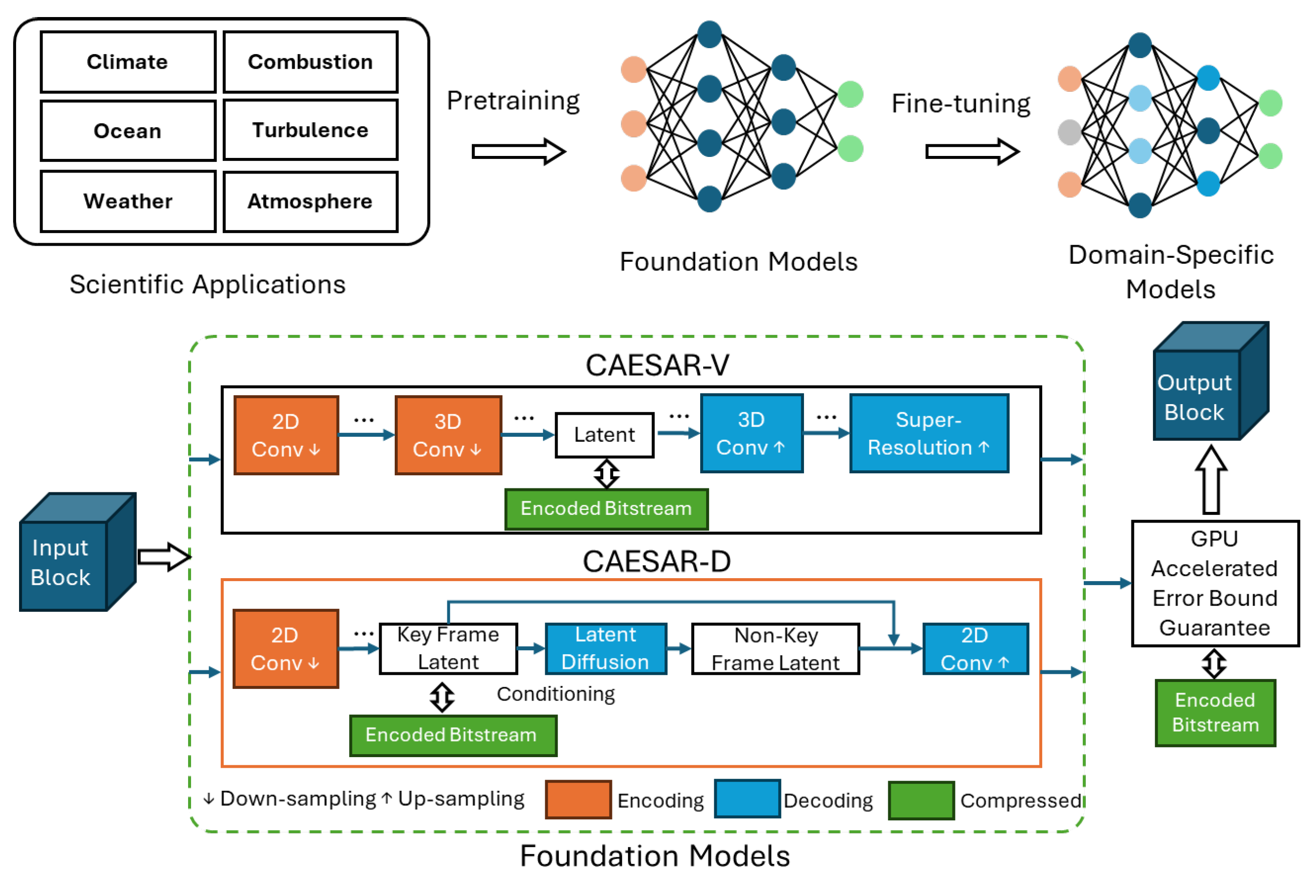
Figure 1. Overview of the CAESAR Framework.
Applsci 15 08977 g001
Figure 2. Overview of the architecture of the transform-based FM. ‘Conv 2D/3D ↓’ denotes a convolution operation with stride 2, while ‘ConvTran 2D/3D ↑’ denotes a transposed convolutional layer. ‘MTD’ refers to merging the temporal dimension, and ‘STD’ refers to splitting the temporal dimension. ‘Q’ represents rounding quantization. ‘AE’ and ‘AD’ denote arithmetic encoding and decoding, respectively. Leaky ReLU is used for nonlinearity.
Applsci 15 08977 g002
Figure 3. The architecture of the BCB module.
Applsci 15 08977 g003
Figure 4. Illustration of the proposed framework. Given a spatiotemporal data block x, each frame is encoded into a latent space using a VAE. Only keyframe latents are retained, quantized, and compressed with a hyperprior. A latent diffusion model then generates latents for the remaining frames by interpolating between keyframes. Finally, all latents are decoded to reconstruct the full data block x ^ .
Applsci 15 08977 g004
Figure 5. Comparison of keyframe selection methods: interpolation, prediction, and hybrid. Top figure shows reconstructions; bottom figure shows per-frame NRMSE.
Applsci 15 08977 g005
Figure 6. Ablation Study for interpolation interval on E3SM dataset.
Applsci 15 08977 g006
Figure 7. Ablation Study for Denoising Step on S3D Dataset.
Applsci 15 08977 g007
Figure 8. Comparison of results on the E3SM, S3D, and JHTDB datasets.
Applsci 15 08977 g008
Figure 9. Comparison of compression ratios for given NRMSE on the E3SM, S3D, and JHTDB datasets.
Applsci 15 08977 g009
Figure 10. Visualization of reconstructed data from CAESAR-D, CAESAR-V, SZ3, and ZFP, all at a compression ratio of approximately 100. Two red rectangles indicate the same region: one shows its location in the full frame, and the other presents a zoomed-in view of that area for detailed comparison.
Applsci 15 08977 g010
Figure 11. Histogram of per-vector NRMSE from E3SM compression with CAESAR-D.
Applsci 15 08977 g011
Table 2. Model Inference Speed on GPU.
DevicesMethodsEncoder (MB/s)Decoder (MB/s)
A100 80 GBCAESAR-V943652
CAESAR-D-128 Steps194216
CAESAR-D-32 Steps194261
CAESAR-D-8 Steps1942203
RTX 2080 24 GBCAESAR-V336251
CAESAR-D-128 Steps8256
CAESAR-D-32 Steps82525
CAESAR-D-8 Steps82593
Table 3. Compression Performance on A100 GPU, RTX 2080 GPU and CPU.
Error BoundA100 GPU (MB/s)RTX 2080 GPU (MB/s)CPU (MB/s)
1 × 10 2 118163652
1 × 10 3 85551412
1 × 10 4 5562916
1 × 10 5 4742263
Disclaimer/Publisher’s Note: The statements, opinions and data contained in all publications are solely those of the individual author(s) and contributor(s) and not of MDPI and/or the editor(s). MDPI and/or the editor(s) disclaim responsibility for any injury to people or property resulting from any ideas, methods, instructions or products referred to in the content.