An Exploratory Study on the Use of Root-Mean-Square Vertical Acceleration Data from Aircraft for the Detection of Low-Level Turbulence at an Operating Airport

Abstract

Low-level turbulence is a meteorological hazard that disrupts the operation of airports and is particularly pronounced at Hong Kong International Airport (HKIA), which is impacted by various sources of low-level turbulence (e.g., terrain disrupting wind flow, sea breeze, and thunderstorms). The possibility of using root-mean-square vertical acceleration (RMSVA) data from Automatic Dependent Surveillance–Broadcast (ADS-B) for low-level turbulence monitoring is studied in this paper. Comparisons are performed between RMSVA and Light Detection And Ranging (LIDAR)-based Eddy Dissipation Rate (EDR) maps and the aircraft-based EDR. Moreover, the LIDAR-based EDR map, aircraft EDR, and pilot report for turbulence reporting are compared for two typical cases at HKIA. It was found that the various estimates/reports of turbulence are generally consistent with one another, at least based on the limited sample considered in this paper. However, at very low altitudes close to the touchdown of arrival flights, RMSVA may not be available due to a lack of ADS-B data. With effective quality control and further in-depth study, it will be possible to use RMSVA to monitor low-level turbulence and to alert pilots if turbulence is reported by the pilot of the preceding flight based on RMSVA. The technical details of the various comparisons and the assumptions made are described herein.

1. Introduction

Low-level turbulence can be hazardous to aircraft operations at an airport. Reports of such turbulence, e.g., from pilots, could aid in the development of quantified turbulence estimates based on measurements of ground-based, remote-sensing meteorological instruments, such as microwave weather radars and Light Detection And Ranging (LIDAR) systems. At present, however, the number of pilot reports is limited. Barry Schwartz [1] notes in their study about the limitation of pilot reports (PIREPs) in the development, calibration, and validation of aviation weather guidance products. In the context of Hong Kong, at Hong Kong International Airport (HKIA), though turbulent flow may be expected due to terrain disruption of the prevailing wind and due to thunderstorms, on average, only one flight in roughly 2000 experiences moderate or greater (MOG) turbulence at low levels. The limited number of reports is one of the major challenges in developing turbulence-alerting algorithms based on wind data derived from meteorological equipment.

The data derived from Automatic Dependent Surveillance–Broadcast (ADS-B) opens up the possibility of supplementing turbulence reports. ADS-B is a surveillance technology used to support air traffic management that allows the aircraft to broadcast its position, altitude, velocity, aircraft identification, vertical rate, etc., via an onboard system [2]. A suitable receiver (either on the ground or in the air) can process the ADS-B information and acquire aircraft information in real time. In this study, the vertical rate in the ADS-B is utilized to understand the aircraft response to low-level turbulence. A metric referred to as the root-mean-square vertical acceleration (RMSVA) may be of particular use for turbulence reporting/monitoring. Bowles and Buck [3] noted in their study that RMSVA is related to the peak accelerations experienced by an aircraft and can be used as a surrogate for peak loads. However, besides meteorological turbulence, RMSVA is susceptible to many other non-meteorological factors, such as maneuvering of the aircraft by the pilot. The impact is particularly significant when the aircraft is close to the ground, performing landing or departure maneuvers. As such, in this study, we attempt to focus on the steady descent/ascent of aircraft and perform quality control on RMSVA data in order to minimize the impacts of manual operation for climb or descent maneuvers and to derive the component of meteorological turbulence.

A common metric for estimating atmospheric turbulence intensity is the Eddy Dissipation Rate (EDR). The EDR is an objective, aircraft-independent indicator of turbulence and is the official International Civil Aviation Organization (ICAO) and World Meteorological Organization (WMO) atmospheric turbulence intensity metric. The EDR estimates the atmospheric turbulence intensity inferred from the cube root of the energy or eddy dissipation rate ($e_w^{1/3}$, unit: ${\mathrm{m}}^{2/3}{\mathrm{s}}^{-1}$) [4]. MacCready [5] suggested in their study that the EDR can be derived from vertical wind velocity or aircraft vertical acceleration using in situ equipment on board aircraft. Both in the study by MacCready [5] and that by Cornman [6], the authors suggested that the EDR is proportional to the root-mean-squared value of aircraft vertical accelerations, though the proportion constant may vary for different aircraft types, aircraft weights, altitudes, etc.

Various efforts have been made to derive turbulence information from ADS-B data. In their study, Kopeć [7] used ADS-B data and wind information from Mode-S interrogation data obtained using a secondary surveillance radar to derive the EDR. In another study, Feliz [8] used the vertical rate and ground speed from the ADS-B and explored the variance within a specified timeframe. Thresholds were set to detect turbulence following a comparative analysis with actual observations.

In the present paper, we describe a comparative analysis for the quality-controlled RMSVA derived from ADS-B data with other independent measurements, such as LIDAR-based EDR maps and aircraft-based EDR data derived from Quick Access Recorders (QARs). The consistency among LIDAR EDR maps, aircraft QAR EDRs, and pilot reports is also demonstrated in two case studies. Although the sample of the data used in the present study is still rather limited, covering only a quarter of a year during winter to spring time, the study period is in fact the peak windshear/turbulence season at HKIA. The results appear promising, and it is hoped that they will provide support for further research on the use of ADS-B data for turbulence monitoring and even alerts in other operating airports.

2. Data

2.1. ADS-B RMSVA Aircraft Data

In this study, to understand the impact of small-scale turbulence on arriving aircraft, the ADS-B data of these aircraft were utilized. Hong Kong Observatory (HKO) installed an ADS-B receiver at Tai Mo Shan Weather Radar Station in June 2016, and it can receive ADS-B data within a range of approximately 600 km from Hong Kong. A metric of root-mean-square vertical acceleration (RMSVA) was calculated by differentiating the vertical rate (available with ADS-B data) over a five-second average gradient. The calculation is shown in Equation (1) below, where $a$: vertical acceleration ($\mathrm{m}{\mathrm{s}}^{-2}$), v: vertical rate ($\mathrm{m}{\mathrm{s}}^{-1}$), and t: timestamps ($\mathrm{s}$). To represent the mean value of a variable over time, the bar notation is used. $\overline{x}$ corresponds to the arithmetic mean of $x$ measured continuously over a five-second interval.

$$a={\displaystyle \frac{\overline{t}\overline{v}-\overline{tv}}{{\left(\overline{t}\right)}^2-\overline{t^2}}}$$

(1)

The results of a previous study demonstrated that the derived RMSVA correlates with turbulence observations reported by pilots [9]. Sharman and Lane [10] noted in their study the relationship between EDR and aircraft root-mean-square normal acceleration and approximate turbulence levels for this metric (

Table 1. Documented thresholds for RMSVA corresponding to turbulence intensity.

Root-Mean-Square Vertical Acceleration [RMSVA] (Unit: g ^)	Turbulence Intensity
0.1 to 0.2	Light
0.2 to 0.3	Moderate
0.3 to 0.6	Severe
≥0.6	Extreme

^{^} The gravitational acceleration g is taken to be 9.81 m/s², the standard value at sea level.

).

2.2. EDR Maps Based on Long-Range LIDAR Data

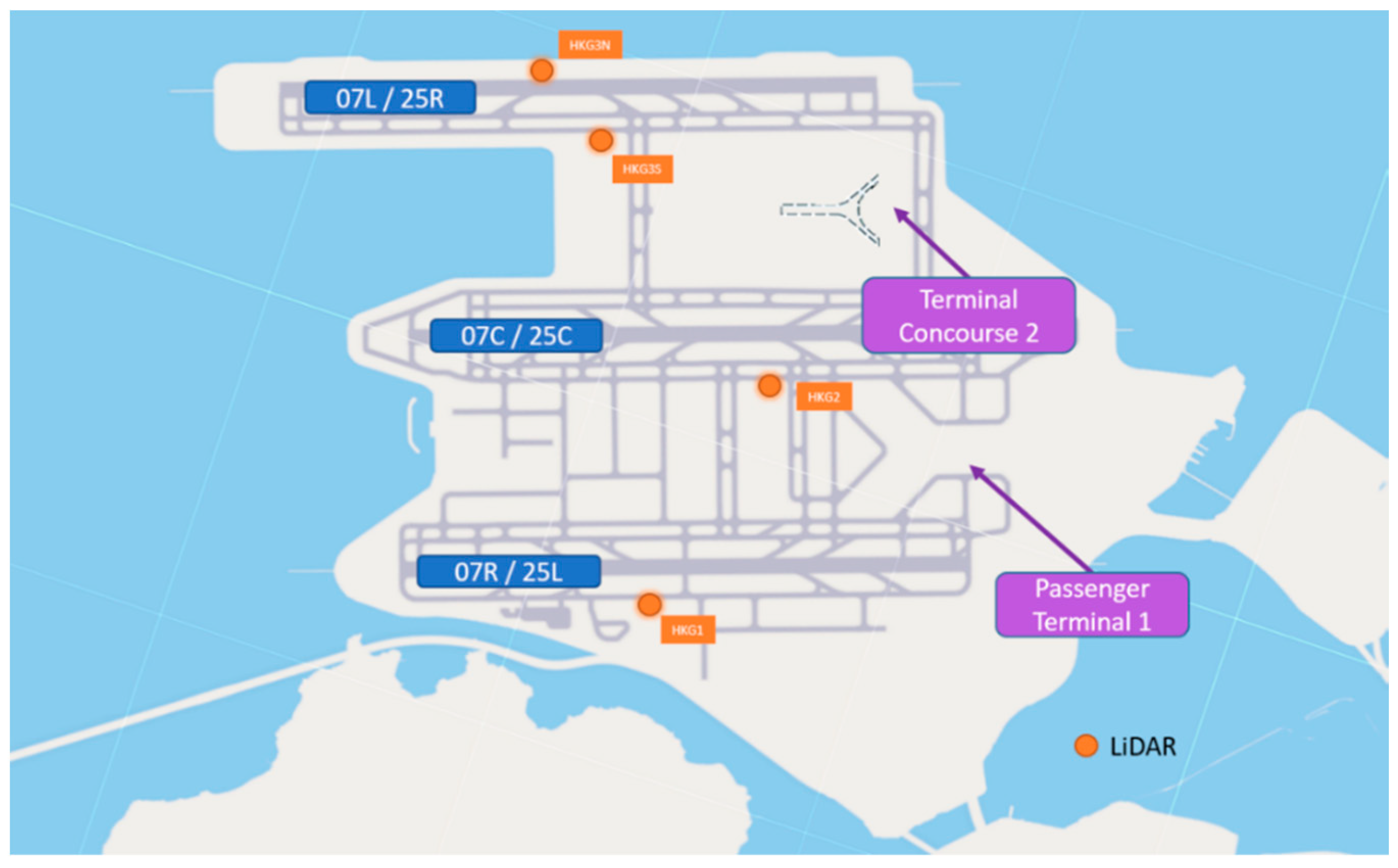
EDR maps are generated in real-time at HKIA, calculated from the radial velocities measured in Plan Position Indicator (PPI) scans of the LIDAR. The radial velocity as a function of range and azimuth in each scan was then fitted to calculate the velocity fluctuation with respect to the fitted plane. Utilizing the velocity fluctuations, the velocity structure function was then calculated and compared with the von Kármán model to determine the EDR. The methodology in generating the EDR maps is described in detail in [11]. HKIA has operated on a three-runway system since 28 November 2024; the three runways are parallel with heading 07/25. HKO has installed at least one LIDAR over each runway for the windshear alerting system in place. The installed LIDARs over HKIA are illustrated in Figure 1. Each LIDAR generates real-time EDR maps and covers all of the departure and arriving corridors of HKIA. The LIDAR-based EDR has been compared with the pilot reports of windshear/turbulence at HKIA based on an extensive dataset covering January to September 2008–2012 [12], and the two datasets are considered to be consistent with one another. The results presented in

Table 2. ICAO Annex 3 turbulence intensity classification.

Eddy Dissipation Rate [EDR] (m2/3s−1)	Turbulence Intensity
0 to 0.1	Nil
0.1 to 0.2	Light
0.2 to 0.45	Moderate
≥0.45	Severe

show the ICAO turbulence intensity classification from the EDR in Annex 3.

2.3. EDR Derived from In Situ Aircraft Measurements

In a collaborative study between HKO and the National Aerospace Laboratory (NLR) in the Netherlands, an algorithm to calculate the EDR from flight data was developed [13,14]. The aim of this method was to objectively derive the wind, windshear hazard factor, and turbulence intensity parameter (i.e., EDR) from QAR data obtained from partner airlines, in addition to pilot reports received. The calculation was specific to the aircraft type to cater for different aerodynamic characteristics across the different types. The calculation software used is called “WINDSTURB”, and it has been used extensively by HKO to analyze flight data collected over HKIA and develop a database of the EDR, serving as the basis for the development of EDR estimates from the various types of meteorological equipment.

Since WINDSTURB supports a limited number of aircraft types and only accepts certain data formats, HKO has recently developed an in-house Python-based (version 3.12) algorithm similar to the WINDSTURB algorithm to calculate EDR and vertical wind based on QAR data. Use of this algorithm would facilitate the processing of a greater number of aircraft types, and the program could be more easily adapted to cater for changes in data format. In essence, different aircraft types would have different constants in the calibration of the true aerodynamic angle of attack. Multilinear regression was performed to derive the constants for other aircraft types. The calibration equation can be found in Equation (4) of [14]. The vertical wind component presented in this study was calculated using Equation (3) from [15] and takes the following form:

$$VWRZ= -TAS\left(\mathit{cos}\theta \mathit{sin}\alpha \mathit{cos}\varphi -\mathit{cos}\alpha \mathit{sin}\theta \right)-IVV$$

(2)

where TAS is the true airspeed ($\mathrm{m}{\mathrm{s}}^{-1}$), $\theta$ is the pitch angle, $\varphi$ is the roll angle, $\alpha$ is the calibrated angle of attack, and IVV is the inertial vertical velocity ($\mathrm{m}{\mathrm{s}}^{-1}$).

The Python program (version 3.12) evaluates the EDR with reference to two methods, i.e., Haverdings and Chan [14], and EDR2W from Kim et al. [16]; both require true air speed and vertical wind in the calculation. The EDR calculated using the two above methods will be referred to as “NLR” and “Spectrum” hereafter. The NLR method is developed based on the WINDSTURB algorithm, employing a running-mean standard deviation calculation of band-pass filtered vertical wind, and the Spectrum method is based on power spectral density (PSD) estimates of vertical wind in a certain frequency range.

The EDR based on the NLR method applies the following equation:

$$EDR={\displaystyle \frac{{\widehat{\sigma }}_w}{\sqrt{1.05{V_a}^{\frac{2}{3}}({{\omega }_1}^{-\frac{2}{3}}-{{\omega }_2}^{-\frac{2}{3}})}}}$$

(3)

The vertical wind component is filtered with a digital band-pass filter with cut-off frequencies of $f_1=0.1 \mathrm{H}$z and $f_2=2 \mathrm{H}$z, ${\omega }_i=2\pi f_i$ is the radian frequency, $V_a$ is the running mean of true air speed filtered by a digital low-pass filter with cut-off frequency $f_2$ within a time window, representing the average flying speed, and ${\widehat{\sigma }}_w$ is the running standard deviation of vertical wind in a time window. The moving time window duration for the running mean or standard deviation parameters is set to 10 s. The selection of values of frequency and time window duration follows the suggestions of Haverdings and Chan [14].

For the EDR based on the Spectrum method, the following equation is applied:

$$EDR={\left({\displaystyle \frac{2\pi }{V_a}}\right)}^{{\displaystyle \frac{1}{3}}}{\displaystyle \frac{\overline{S_i\left(f\right)f^{\frac{5}{3}}}}{C_K^{-1}}}$$

(4)

The moving time window duration in the Spectrum method follows the NLR method, i.e., 10 s. $V_a$ is the mean true air speed in the time window, $C_K$ is the Kolmogorov constant set as 0.65, and $S_i\left(f\right)$ is the PSD of the vertical wind component at a specific frequency $f$, estimated using fast Fourier transform. PSD values within the same frequency domain as the NLR method, i.e., between 0.1 to 2 Hz (inclusive), were adopted in the calculation. The Kolmogorov constant in Equation (4), which could be viewed as the scaling multiple, was adjusted slightly from that used by Kim et al. [16] based on previous comparison studies. The values of frequencies and time window duration in our Spectrum method follows the NLR method to ensure a fair comparison among the methods on the same QAR dataset.

3. Comparison Between RMSVA from Aircraft and LIDAR EDR Maps

In this section, we examine the EDR derived from the network of LIDAR installed on the HKIA and RMSVA derived from ADS-B data from landing aircraft. The analysis was performed over individual arrival corridors.

The study covers the period of January to March 2025, during winter to spring time in Hong Kong. The prevailing wind type in Hong Kong in the study period is easterlies [17]; therefore, the arriving corridor 07 from the west is more frequently used. As HKIA is built on an island surrounded by the sea, during days with prolonged sunshine, sea breeze effects may occur, and a westerly sea breeze will lead to the use of 25 arrival corridors from the east [18]. It is worth noting that 07L is much further north, and the approaching corridor is positioned primarily over the sea. The 07R is situated more southerly and is closer to the Lantau Peak with a height of 934 m; in comparison, the 25R corridor is closer to the Tai Mo Shan peak further east, with a height of 957 m, the highest surrounding Hong Kong.

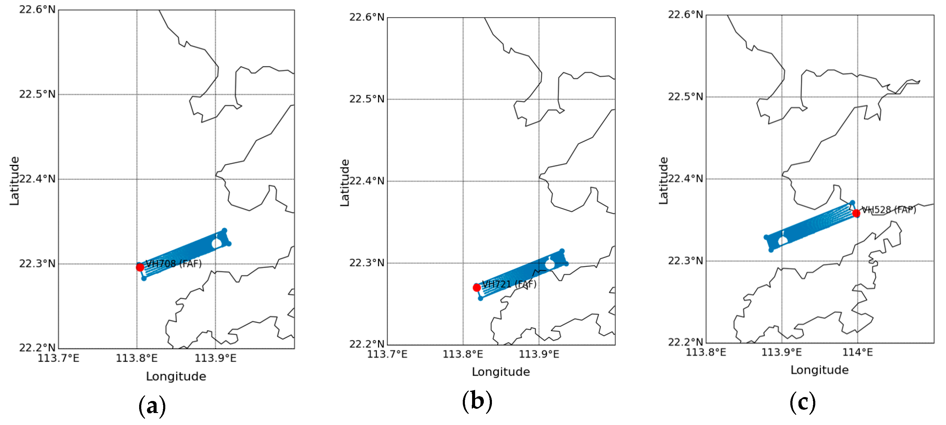
As we focus on the landing glide path during the descent in this study, only EDR values from LIDAR within the landing path were extracted. The entry point was taken as the final approach point (FAP) or the final approach fix (FAF) of the respective arriving corridors [19]. In Figure 2, the maps of the region of interest used in this study for different arrival corridors are shown. The 90th percentile of EDR values within the respective interest region from each LIDAR scan was extracted. For 07L and 25R, the LIDAR HKG3S located on the southern side of the north runway was used, including a LIDAR scan with an angle of 3.1°. For 07R, the LIDAR HKG1 located at the south runway was used, including a LIDAR scan with an angle of 3.2°. The 90th percentile values were chosen to provide a more robust measure that accounts for the EDR values over the region of interest against outliers, which may possibly be derived from the noise of the LIDAR scans.

The landing aircraft were first grouped by their landing corridors extracted from the HKIA Airport Operational Database. For each landing aircraft, the peak RMSVA experienced during its descent was then extracted. To exclude the impact of aircraft maneuvers, only those RMSVAs calculated after FAP and FAF were extracted (i.e., below 1500 ft for 07L, below 1600 ft for 07R, and below 1700 ft for 25R). Moreover, high RMSVA values are recorded when an aircraft performs go-around procedures with the rapid manual climb initiated by the pilot. Therefore, those aircraft that have maximum RMSVA values during positive vertical rate (i.e., climbing) were removed from the dataset. Only steadily descending aircraft are included to analyze the possibility of turbulence being encountered and its impact on the RMSVA parameter. The results presented in

Table 3. The number of aircraft utilized in this study from arrivals.

	07L	07R	25R
January	9646	298	1377
February	8397	149	1179
March	7950	237	3167
Total	25,993	684	5723

below show the number of aircraft utilized in this study for 07L, 07R, and 25R arrivals. As the number of flights landing on 25L was very low (fewer than 230 flights) from January to March 2025, the 25L arrival corridor was not investigated.

Noting that there are a variety of aircraft types and loading for landing aircraft at HKIA, and the LIDAR scans may not coincide with the exact timing that an aircraft lands, an hourly interval was chosen to represent the general atmospheric conditions during the investigation. In any given hour, there are around 34 aircraft landing and four LIDAR scans.

To investigate the hourly and monthly characteristics of the hourly peak of RMSVA and the 90th percentile of LIDAR EDR, comparative plots for runway 07L arrivals are shown in Figure 3. Only runway 07L is shown as it possesses more balanced data across months, and data is available for every hour; it also serves as the major arrival runway during the winter to early springtime at HKIA. Figure 3a shows that the EDR derived from LIDAR has higher variability and values as compared with RMSVA. LIDAR EDR showed higher values in January as compared with February and March, while the monthly distribution of RMSVA was similar across the months. The results presented in Figure 3b illustrate similarities in the diurnal features between RMSVA and LIDAR EDR. In January, the values peak at 02 to 07 UTC (10 to 15 LT) with a second minor peak at 19 to 22 UTC (3 to 6 LT). In February, the values are generally lower. In March, the values peak at 03 to 06 UTC (11 to 14 LT) with a second minor peak at 21 to 22 UTC (5 to 6 LT). Note that the statistics of RMSVA depend on the number of aircraft arriving on that runway within that particular hour and can be affected by the density of air traffic.

Next, we investigated the hourly peak of RMSVA and the 90th percentile of LIDAR EDR via scatter plots. The R-squared value is the coefficient of determination, which quantifies how much variation is explained in the dependent variable by the independent variable in a model. A greater R-squared value infers a better model. The p-value helps to determine whether the relationships observed in a model are statistically significant, which tests the null hypothesis against the alternative. A lower p-value indicates greater significance, and a commonly employed significance level is 0.05.

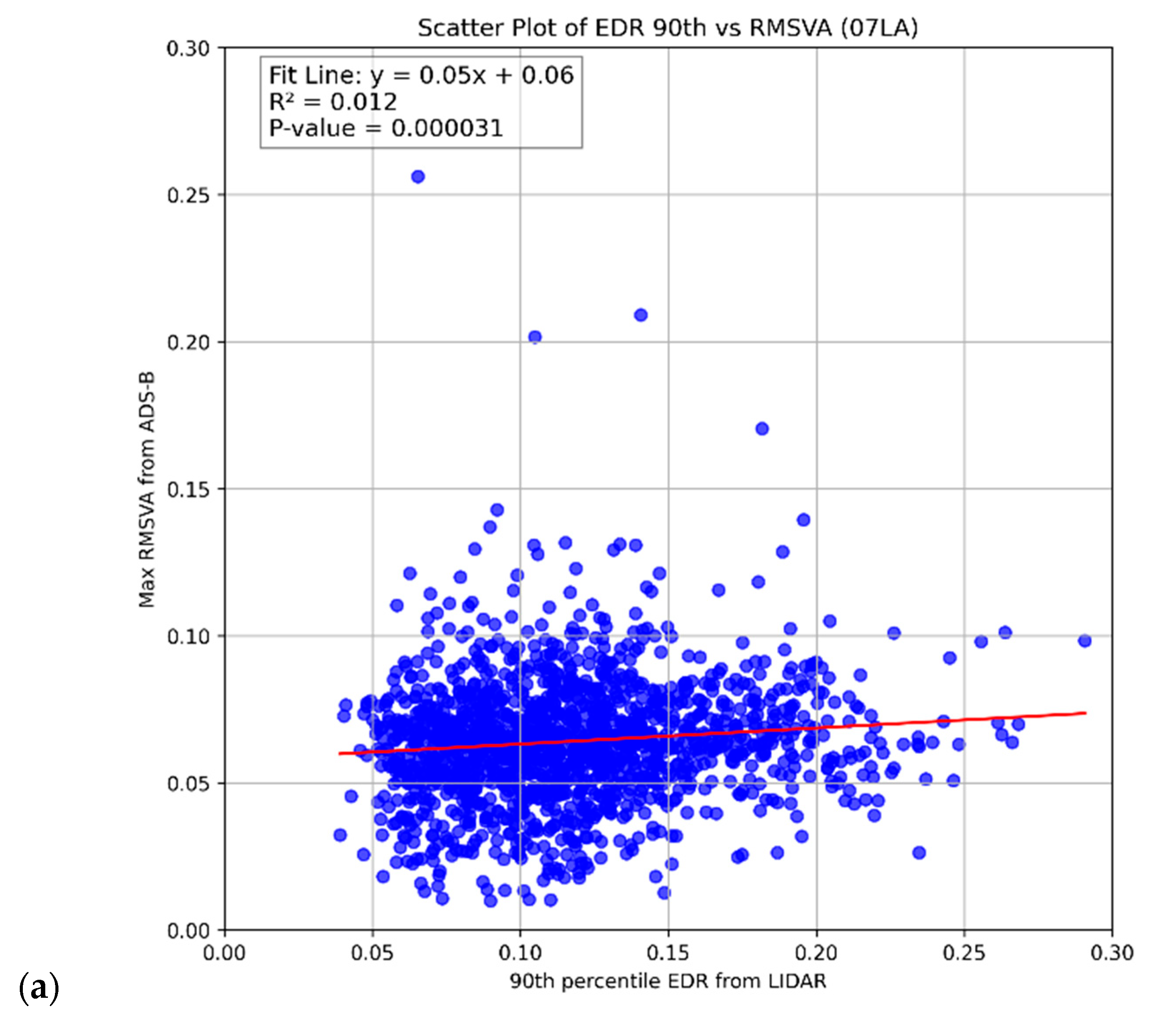
Scatter plots of hourly maximum RMSVA and LIDAR EDR are illustrated in Figure 4. It was observed that there is a weak positive relationship between the hourly maximum RMSVA and the 90th percentile of LIDAR EDR over 07LA (Figure 4a) and 07RA (Figure 4b). Although the R-squared value is low, meaning that only a small part of the variation in the EDR is explained by RMSVA, the p-value is small, meaning that RMSVA has a statistically significant impact in explaining the EDR. Comparing Figure 4a,b suggests that, in general, the LIDAR EDR values are higher over 07RA as compared with 07LA due to its proximity to the Lantau Peak situated south of the runway. Regarding 25RA (Figure 4c), no relationship can be identified, possibly due to the much lower number of aircraft landing on this runway; of note, the p-value was also considerably higher.

Only weak positive relationships were identified between hourly maximum RMSVA and LIDAR EDR, which can be attributed to a few limitations of this study. First, although some quality control measures were implemented, RMSVA may have inevitably included some aspects of aircraft maneuvers initiated by pilots that are not attributed to the atmospheric conditions. Secondly, the vertical acceleration experienced by the aircraft can vary for different aircraft types. In addition, the von Kármán model was utilized for the calculation of LIDAR EDR, which proposes an energy spectrum model for isotropic turbulence. Karasewicz [20] has suggested that shortly before and after sunset, non-equilibrium turbulence is present, which may lead to the underestimation of the EDR from LIDAR.

4. Comparison of RMSVA and Aircraft-Based EDR

Both RMSVA and EDR are derived from aircraft data, though from different sources; they can be compared to determine whether any correlations are present. In this study, we considered a limited sample of aircraft data for two cases, namely, severe turbulence associated with a squall line near HKIA on 15 March 2025, involving five aircraft, and moderate turbulence in a sea breeze case at HKIA on 9 March 2025, involving four aircraft. Time series of RMSVA and EDR were obtained for each aircraft and used for direct comparison purposes.

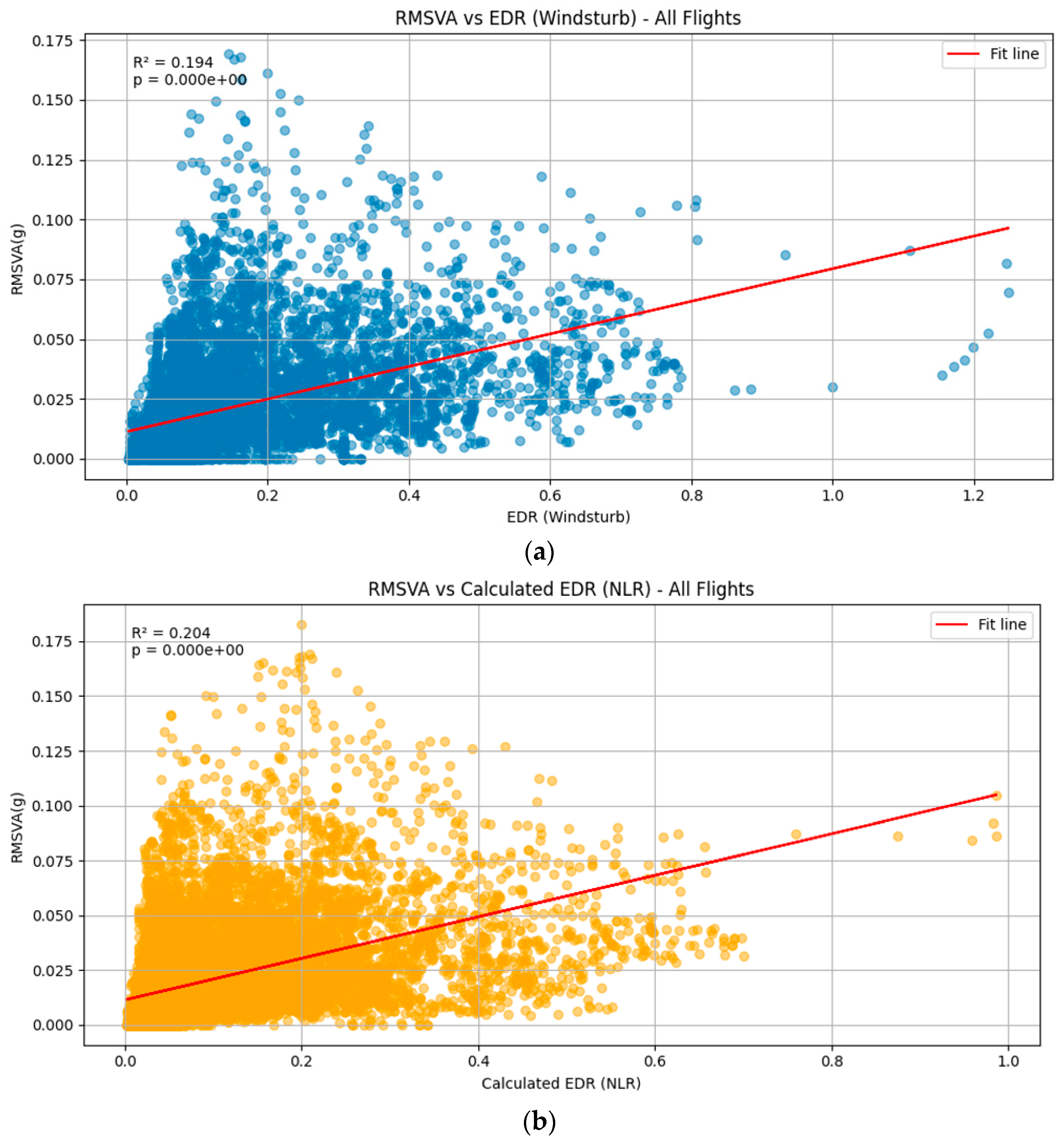
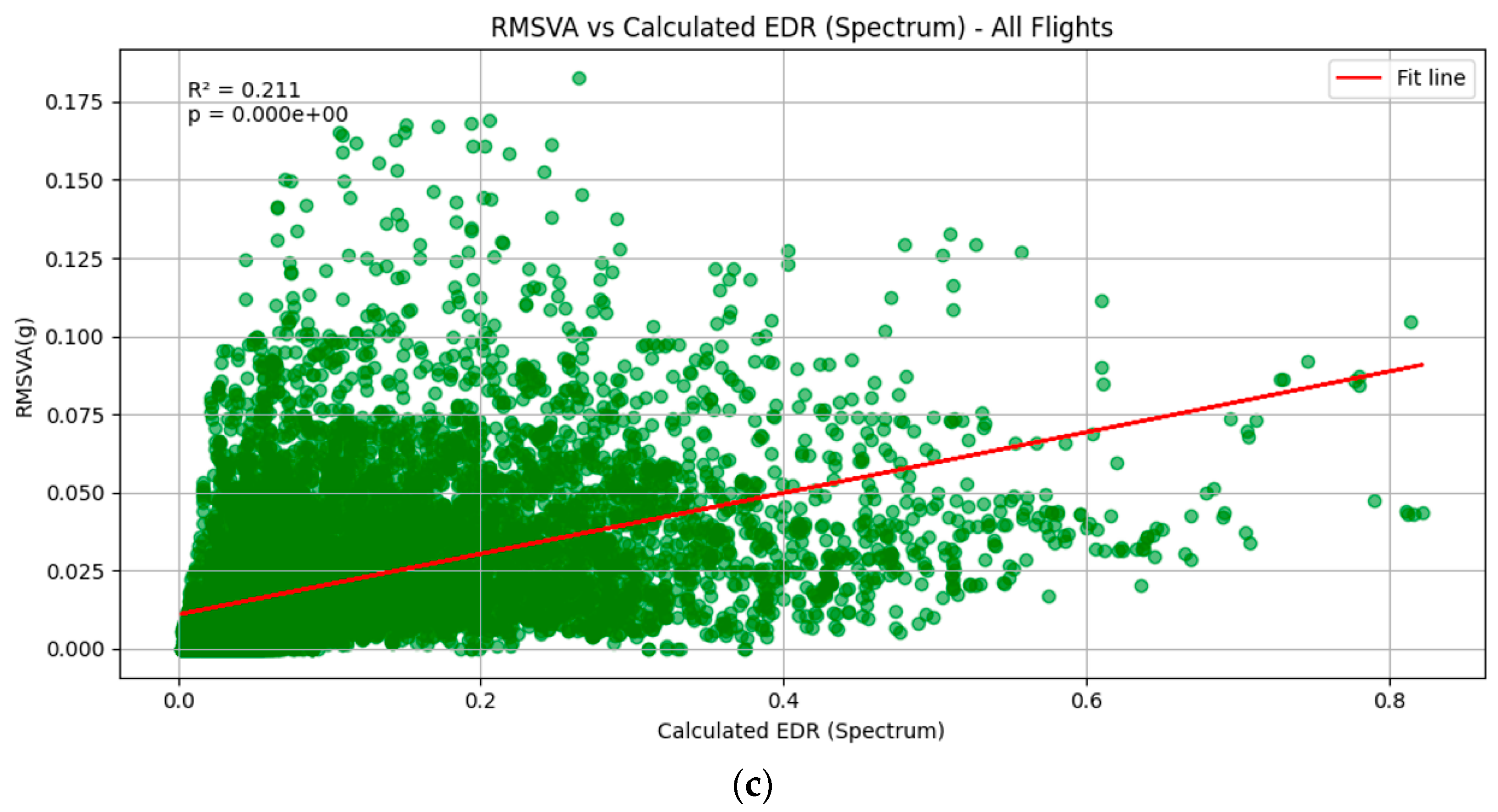
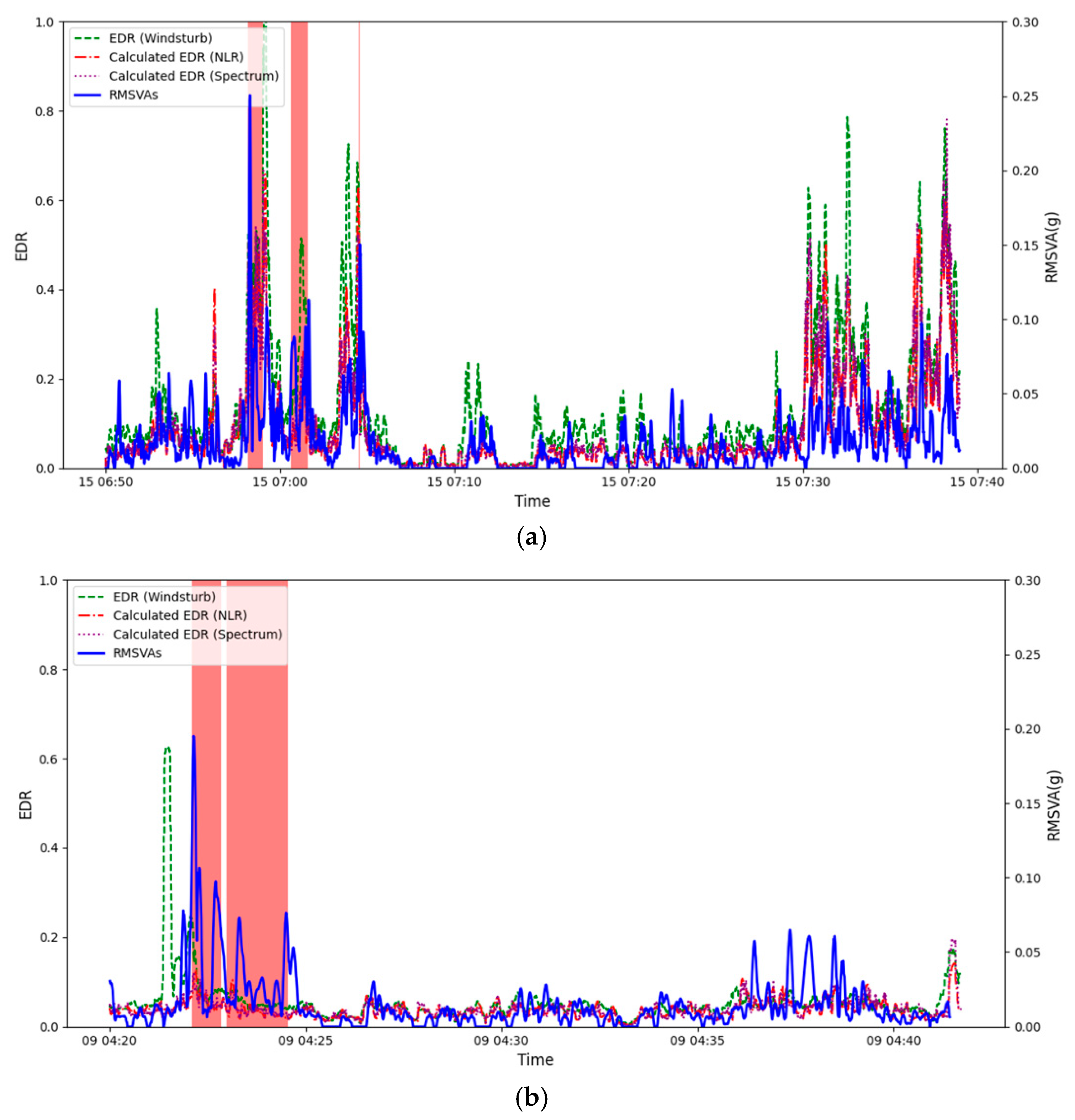
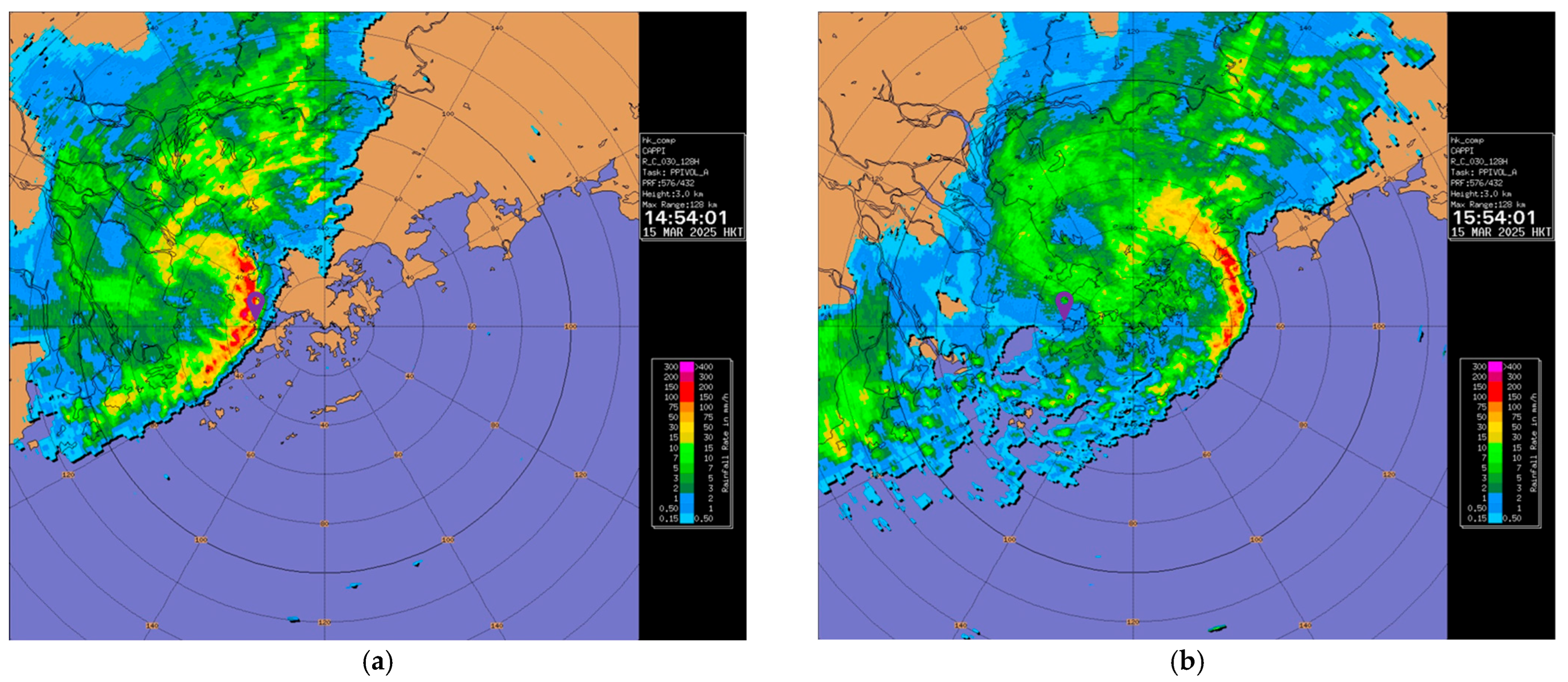
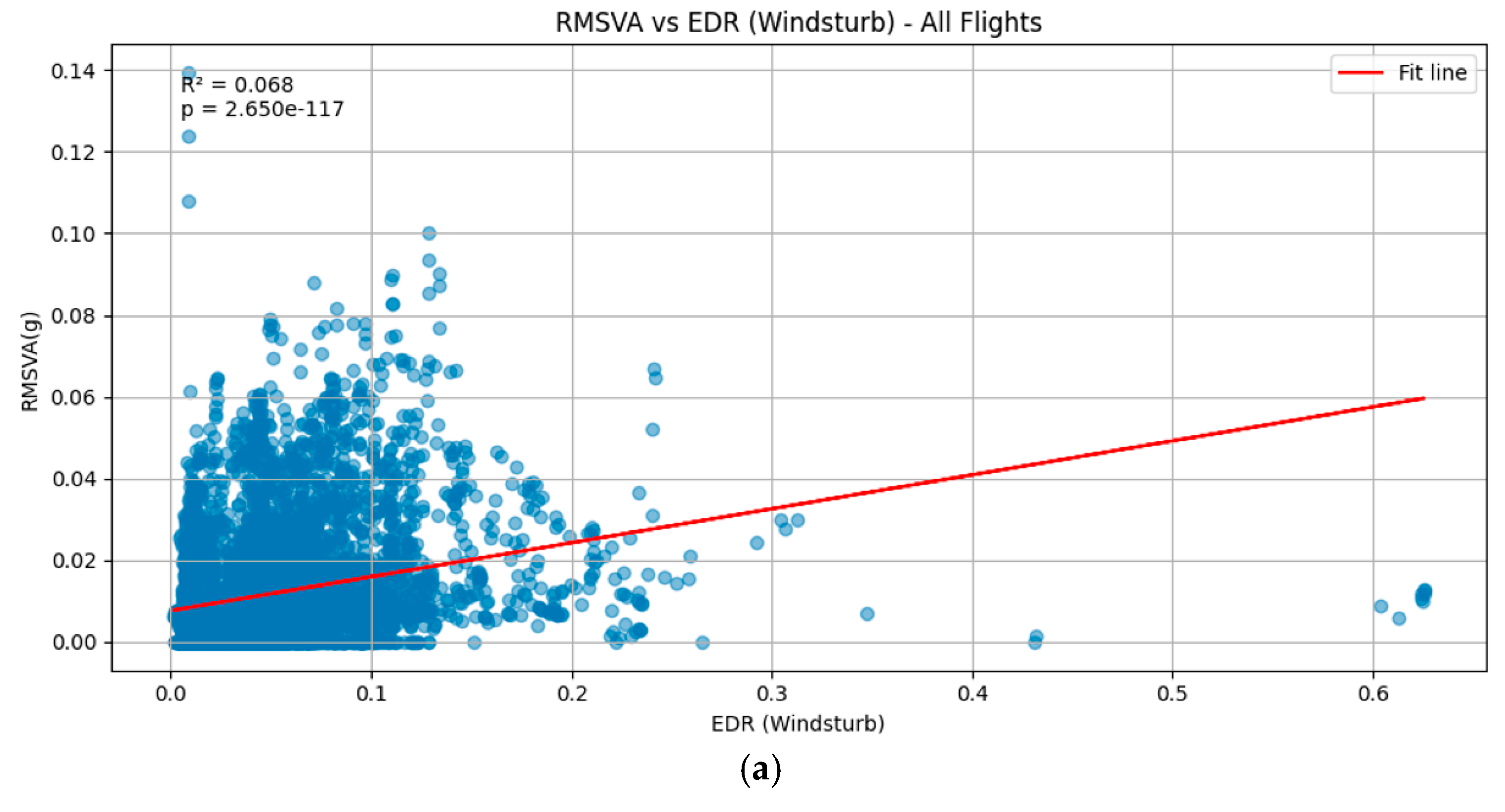
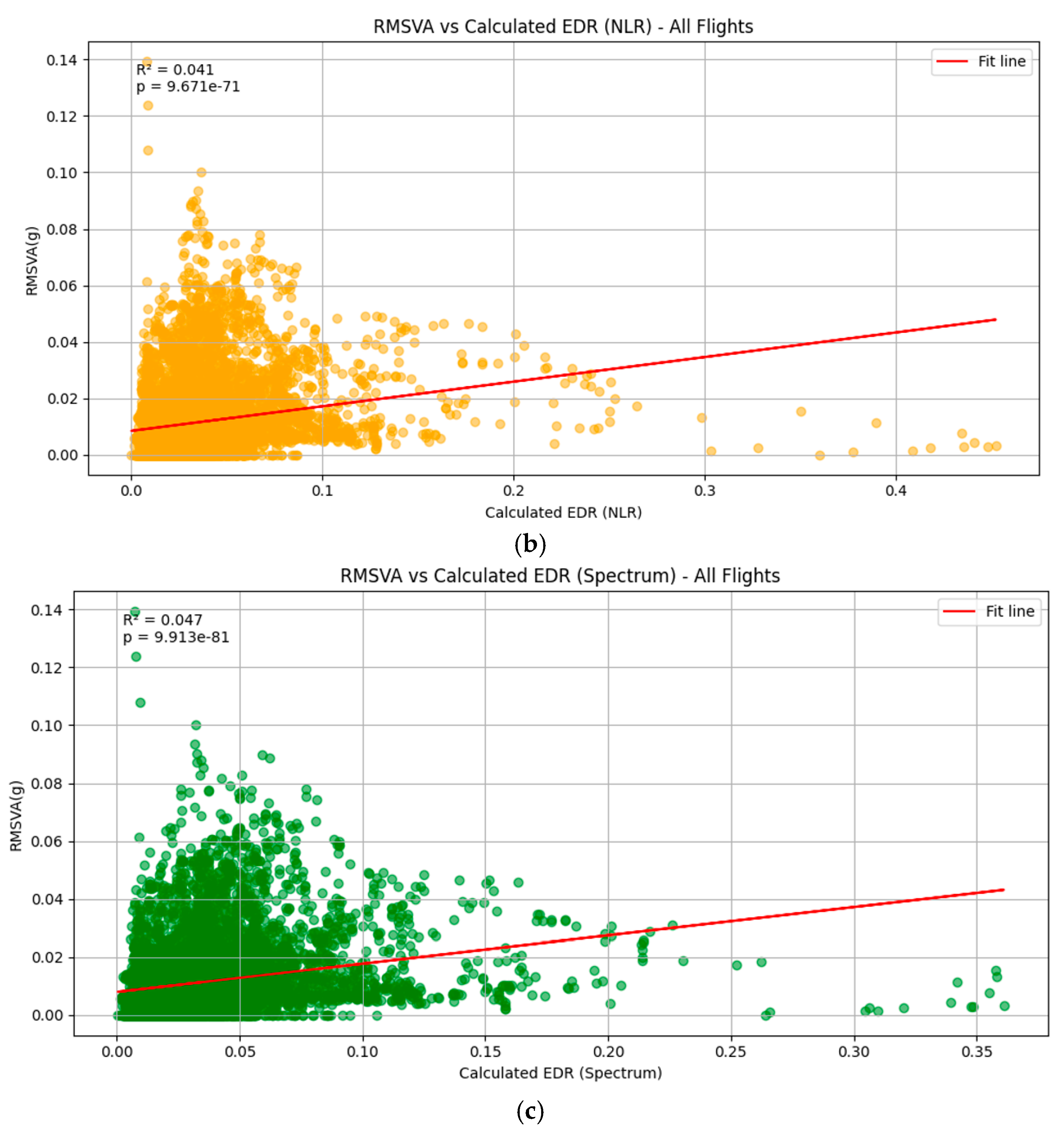
The results of the squall line case are shown in Figure 5. Three methods for calculating the EDR based on aircraft data are considered, namely, WINDSTURB (Figure 5a), NLR (Figure 5b), and Spectrum (Figure 5c). It can be seen that the RMSVA and various estimates of the EDR are weakly correlated, and the results are statistically significant. It was also observed that the RMSVA variation is much smaller than the EDR values calculated. An example flight is shown in Figure 6a. The EDR can reach 1.0 m^2/3s⁻¹, and RMSVA also reaches high values during the areas highlighted in red. The aircraft may experience low-level turbulence before performing go-around procedures. In Figure 6a, it can also be observed during the second landing, around 07:30 to 07:40, that both EDR values and RMSVAs showed higher values, indicating the possibility of low-level turbulence after the passage of the squall line. The radar imagery on 15 March 2025 is shown in Figure 7 for the reader’s reference.

The comparison results for the sea breeze case on 9 March 2025 are shown in Figure 8a–c. An example flight is shown in Figure 6b. Compared to the squall line case, the comparison result is less satisfactory, with generally lower correlation coefficients, though the results are still statistically significant. From the example flight shown in Figure 6b, it can be seen that the areas of moderate turbulence as recorded by means of the EDR may not match the times of larger values of RMSVA.

It can be seen that the results presented in both Figure 5 and Figure 8 show a relatively large spread in the scatter plots for RMSVA and aircraft-based EDR. This finding can be attributed to the following factors: (1) The difference in time scales and frequency between the ADS-B data (around 1 to 2 Hz) and the aircraft data (around 4 Hz) obtained may be attributed to the differentiation in the turbulence intensity derived [21]. (2) In this paper, three proposed algorithms for deriving the EDR from aircraft QAR data are presented, and some subtle differences can be observed from the time series in Figure 6. There may also be some deviations from the true atmospheric conditions for the EDR derived from aircraft QAR data. (3) Pilot aircraft maneuvers may interfere with RMSVA, which may not be solely attributed to the atmospheric conditions.

5. Case Studies Comparing Pilot Reports

In this section, we present some case studies with pilot reports on turbulence recorded. A pilot report includes the time, altitude, location, and intensity of the occurrence of in-flight hazardous weather such as windshear and turbulence. These reports are valuable in understanding the actual conditions observed or experienced in the aircraft and could serve as a basis for follow-up studies. However, pilot reports of turbulence are generally subjective and aircraft-type dependent, and thus, they must be supplemented by other observations and measurements [22].

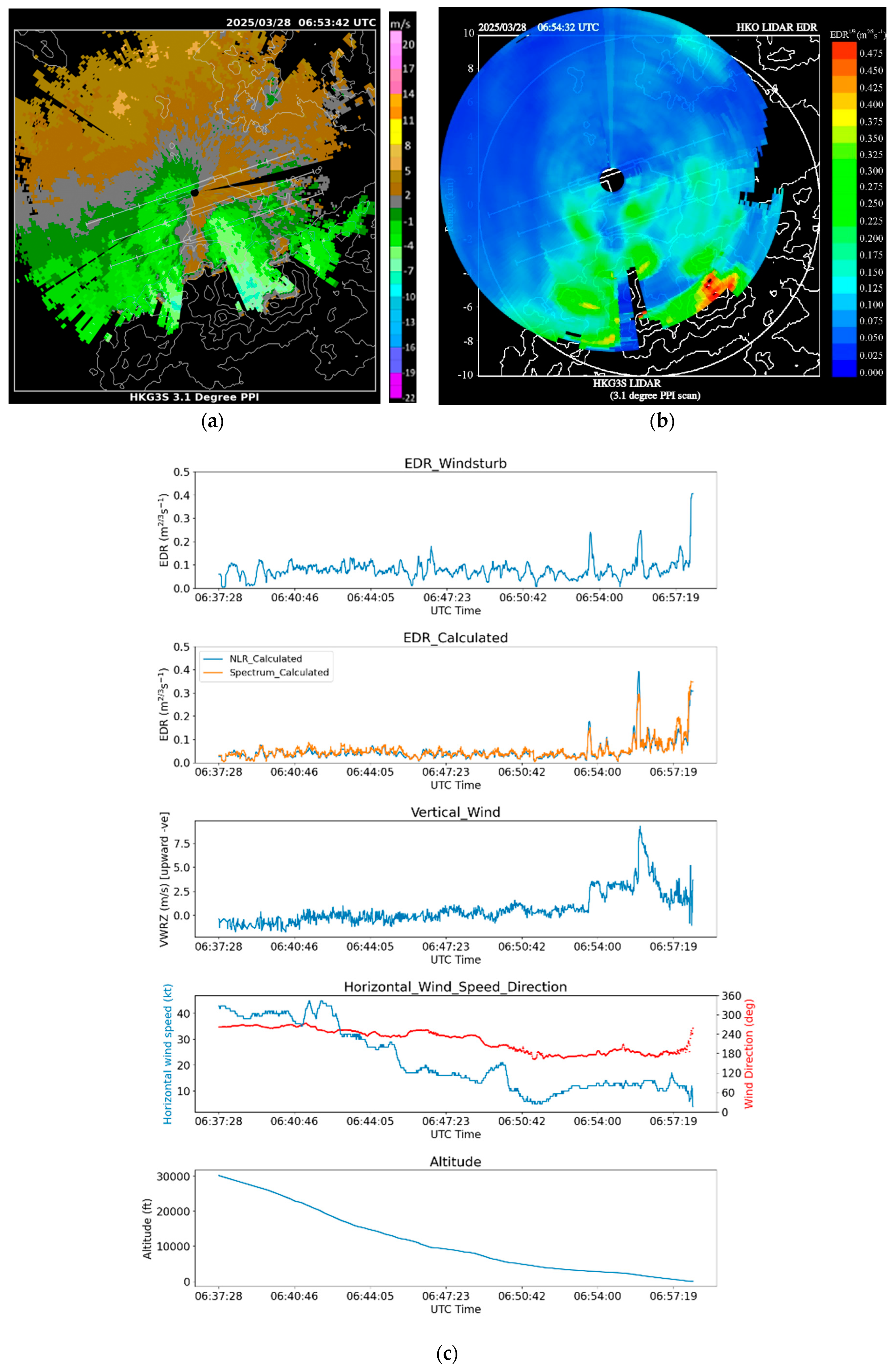
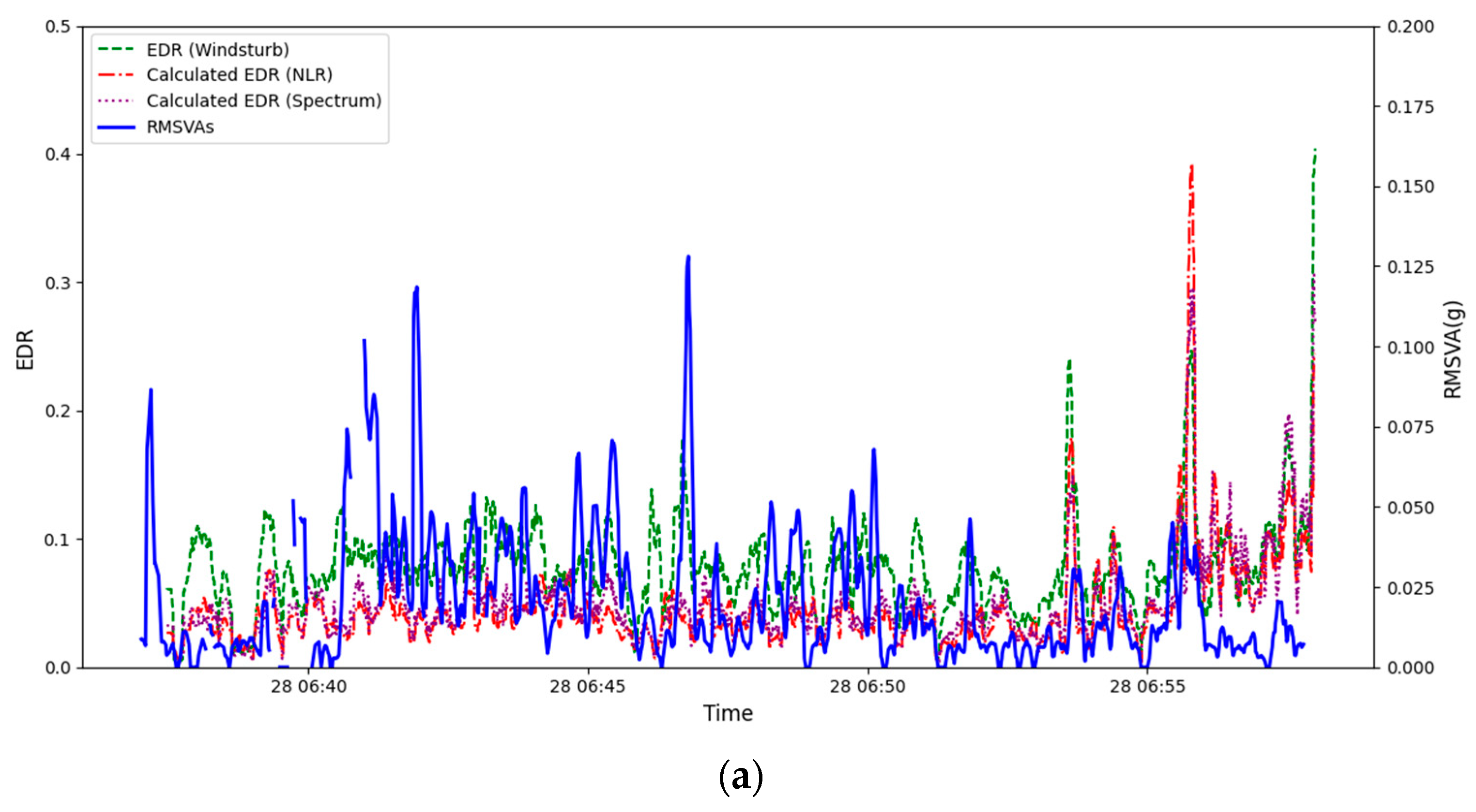
The first case is a pilot report of moderate turbulence for terrain-disrupted airflow on 28 March 2025 at an altitude of 10 ft, shortly before touchdown along the arrival runway corridor to the west of the north runway (07LA). The LIDAR plan position indicator (PPI) imagery is shown in Figure 9a. It can be seen that higher-wind-speed areas were present in the valleys, and a weaker wind/reverse flow can be found downstream of the peaks. For 07LA, moderate turbulence could be found in the EDR map (Figure 9b) in association with the jet from the valley. The pilot reported encountering moderate turbulence upon arrival at 07LA at that time. The corresponding flight data can be found in Figure 9c. The calculated EDR from WINDSTURB, NLR, and Spectrum all showed the EDR rising to around 0.3–0.4 m^2/3s⁻¹ in the last 10 s before touchdown, corresponding to a moderate turbulence event. From the vertical velocity, upward motion of roughly 5 m/s could be identified at the time of moderate turbulence in the time series. Such upward motion close to the touchdown on the arrival runway corridor may be hazardous to the arriving aircraft. Some peaks in the RMSVA can be observed combined with peaks in the EDR (Figure 10a). However, the RMSVA could not be calculated for the turbulence case in the pilot report because the vertical rate was not broadcast through ADS-B, likely due to proximity to landing.

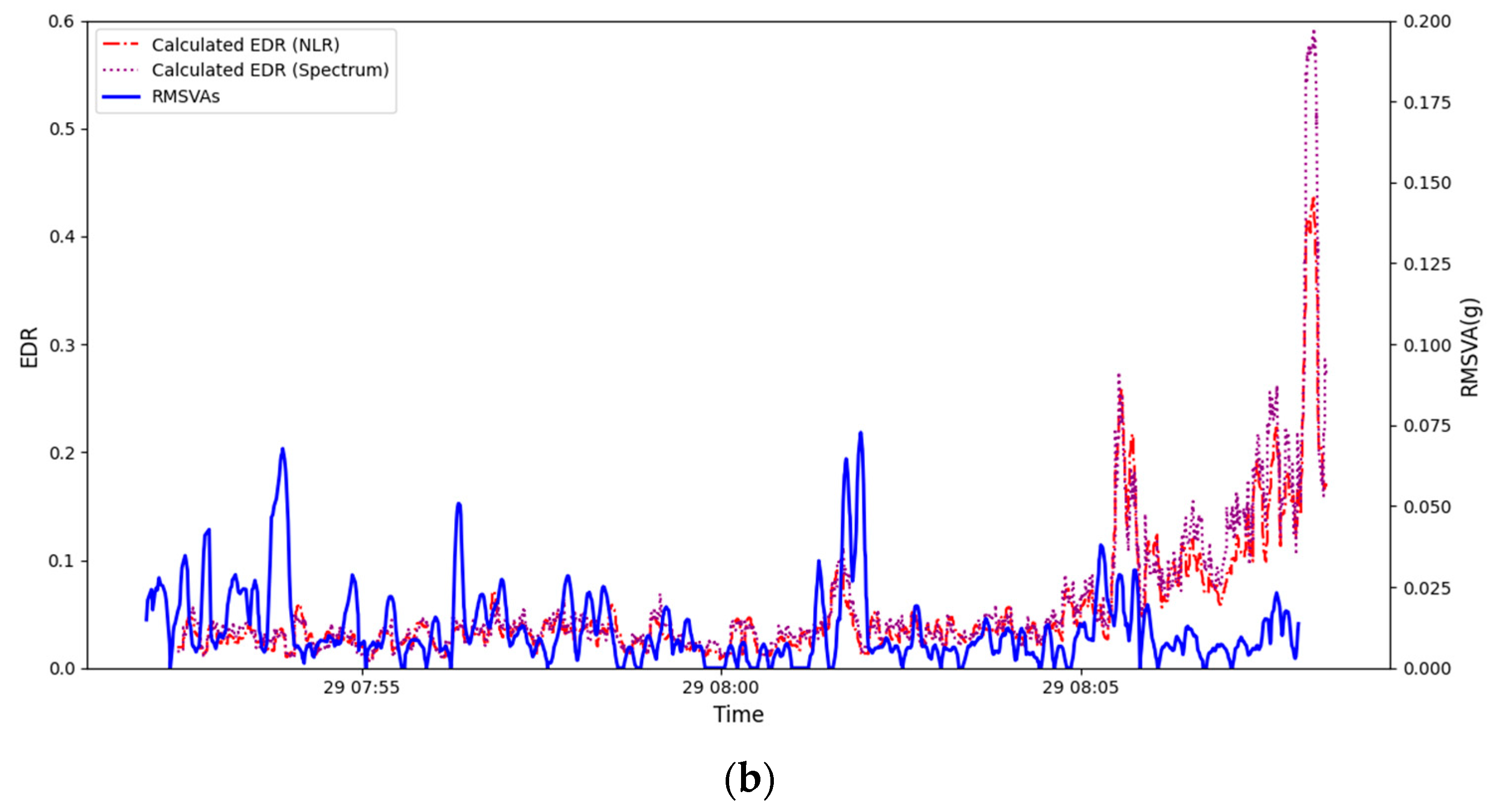
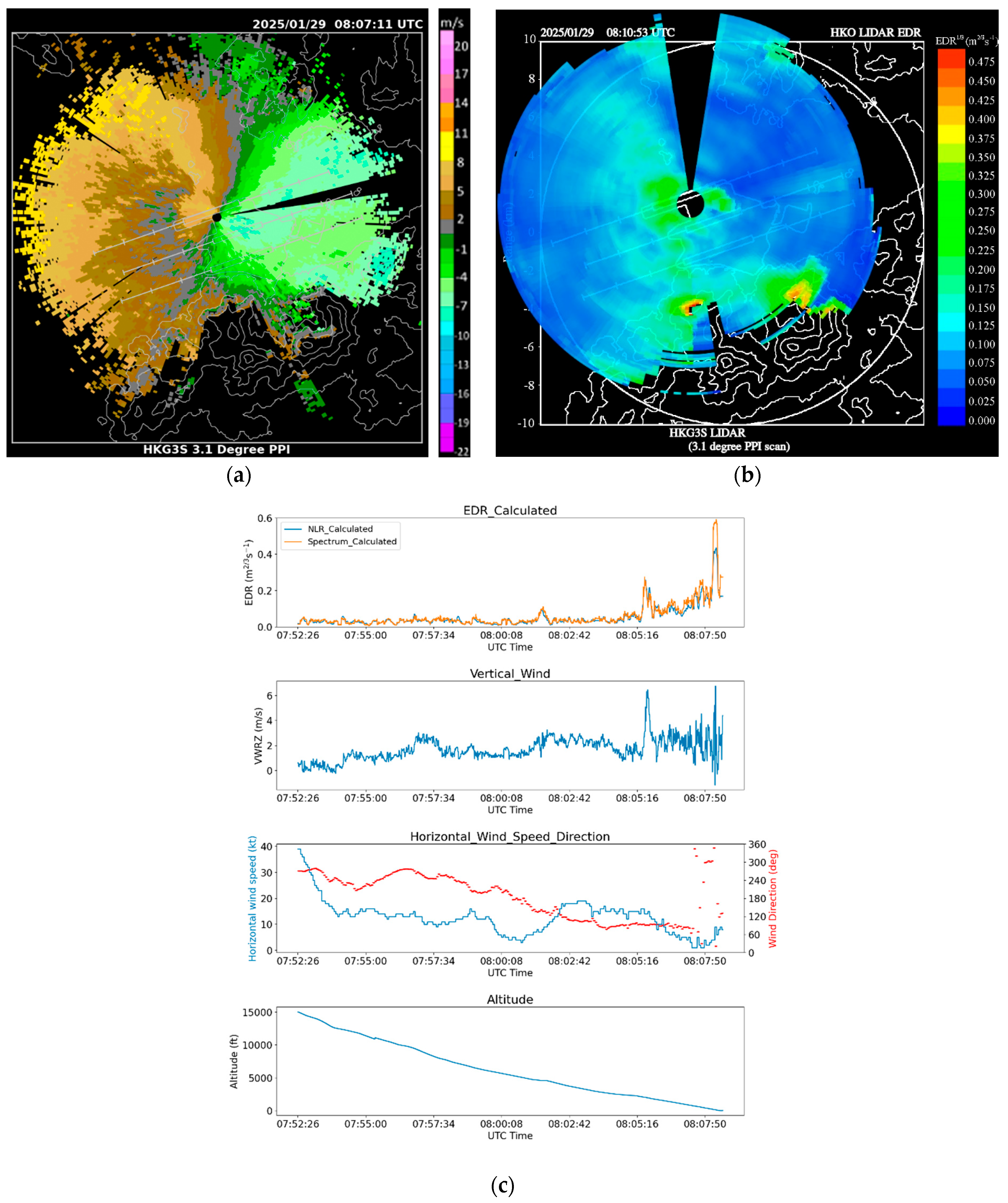
The second case is also a pilot report of moderate turbulence on 29 January 2025 at an altitude of 100 ft in the final nautical mile of the arrival corridor 07LA. LIDAR PPI imagery (Figure 11a) shows that background winds were generally easterly in the LIDAR range; however, a westerly sea breeze was also observed over the westernmost part of HKIA, over which the aircraft flew while descending. Both the easterly and westerly flows were rather turbulent, with patches of high velocity along the path. The EDR map (Figure 11b) also supports this observation, showing a greenish area of the EDR close to 0.3 m^2/3s⁻¹ over the north runway. From the corresponding flight data in Figure 11c, the calculated EDR from NLR and Spectrum reached a maximum of 0.44 and 0.59 m^2/3s⁻¹, respectively, before the plane landed in the last 20 s of the time series; it is evident that a moderate-to-severe turbulence event had taken place. WINDSTURB EDR does not support the calculation of aircraft type in this case. Although the calculated EDR values from flight data were slightly higher than those of the LIDAR EDR map, the abrupt rise in EDR coincided with the time when the flight entered the final mile of 07LA. There was also a large fluctuation in vertical wind, and upward motion exceeded 6 m/s. The RMSVA time series for the same period was also studied (Figure 10b); a similar conclusion as the previous case could be drawn, and the RMSVA corresponding to the pilot report was not available at very low altitudes.

The pilot reports, aircraft-based EDR, LIDAR EDR maps, and RMSVA peaks are all generally consistent for these two cases. However, these two cases also demonstrate a limitation of RMSVA derived from ADS-B, wherein there will be signal loss at very low altitudes with missing information.

6. Conclusions

In this study, the feasibility of using RMSVA based on ADS-B data from aircraft for low-level turbulence reporting is explored. Comparison of ADS-B data with various data sources was conducted, namely, between RMSVA and LIDAR-based EDR, between RMSVA and aircraft QAR-derived EDR, and among LIDAR-based EDR, aircraft QAR-derived EDR, and pilot reports. Although the samples only span a typical windshear season (winter to spring) in a particular year (2025), with only a few case studies conducted, it can be concluded that RMSVA has a weak correlation with LIDAR-based EDR and aircraft QAR-derived EDR, and this finding may possibly indicate the presence of turbulence. However, due to turbulence occurring at very low altitudes and close to touchdown of arriving flights, ADS-B-derived RMSVA may not be able to reflect these cases when the vertical rate is not broadcast. Ground-based and remote sensing measurements, in addition to flight data, are necessary to examine such turbulence cases. Further research efforts (e.g., combination with other observations, aircraft type characteristics, and implementing effective quality control) on the application of RMSVA data for turbulence monitoring (e.g., in the development of other meteorological equipment-based EDR products) and alerting (i.e., passing the suspected turbulence from a preceding flight to the latter flights) are possible. Further studies should also be conducted to cover other windshear seasons at HKIA (e.g., summer) and in different years in order to develop a larger sample for statistical analysis. Based on the availability of a large amount of EDR data for HKIA (e.g., based on aircraft data itself or based on meteorological remote sensing instruments), any attempt to calculate the EDR from ADS-B data could be studied in depth through extensive comparison, and the results of such studies could be reported in the future.

References

1. Schwartz, B. The quantitative use of PIREPs in developing aviation weather guidance products. Weather Forecast. 1996, 11, 372–384. [Google Scholar] [CrossRef]
2. International Civil Aviation Organization. Manual on Airborne Surveillance Applications, Doc 9994, 2nd ed.; ICAO: Montreal, Canada, 2020; ISBN 978-92-9265-322-4. Available online: https://www.icao.int. (accessed on 16 April 2025).
3. Bowles, R.L.; Buck, B.K. A Methodology for Determining Statistical Performance Compliance for Airborne Doppler Radar with Forward-Looking Turbulence Detection Capability; No. NASA/CR-2009-215769; Langley Research Center: Hampton, VA, USA, 2009. [Google Scholar]
4. Sharman, R.D.; Cornman, L.B.; Meymaris, G.; Pearson, J.; Farrar, T. Description and derived climatologies of automated in situ eddy-dissipation-rate reports of atmospheric turbulence. J. Appl. Meteorol. Climatol. 2014, 53, 1416–1432. [Google Scholar] [CrossRef]
5. MacCready, P.B., Jr. Standardization of gustiness values from aircraft. J. Appl. Meteorol. Climatol. 1964, 3, 439–449. [Google Scholar] [CrossRef]
6. Cornman, L.B.; Morse, C.S.; Cunning, G. Real-time estimation of atmospheric turbulence severity from in-situ aircraft measurements. J. Aircr. 1995, 32, 171–177. [Google Scholar] [CrossRef]
7. Kopeć, J.M.; Kwiatkowski, K.; de Haan, S.; Malinowski, S.P. Retrieving atmospheric turbulence information from regular commercial aircraft using Mode-S and ADS-B. Atmos. Meas. Tech. Discuss. 2016, 9, 2253–2265. [Google Scholar] [CrossRef]
8. Feliz, E. Using ADS-B data to Detect Turbulence. Aireon–Space-Based ADS-B Global Air Traffic Surveillance and Tracking. Available online: https://aireon.com/using-ads-b-data-to-detect-turbulence/ (accessed on 24 September 2024).
9. Leung, C.Y.Y.; Leung, H.T. Estimating en-route turbulence using ADS-B aircraft data. In Proceedings of the EMS Annual Meeting 2024, Barcelona, Spain, 1–6 September 2024. EMS2024-635. [Google Scholar] [CrossRef]
10. Sharman, R.; Lane, T. Aviation Turbulence; Springer International Publishing: Cham, Switzerland, 2016; Volume 10. [Google Scholar]
11. Chan, P.W. Generation of an eddy dissipation rate map at the Hong Kong International Airport based on Doppler lidar data. J. Atmos. Ocean. Technol. 2011, 28, 37–49. [Google Scholar] [CrossRef]
12. Hon, K.K.; Chan, P.W. Application of LIDAR-derived eddy dissipation rate profiles in low-level wind shear and turbulence alerts at Hong Kong International Airport. Meteorol. Appl. 2014, 21, 74–85. [Google Scholar] [CrossRef]
13. de Bruin, A.C.; Haverdings, H. Proposal for a Method to Compute Eddy Dissipation Rate from Flight Data Recorder Data; NLR-CR-2007-137; National Aerospace Laboratory: Amsterdam, The Netherlands, 2007; p. 29. [Google Scholar]
14. Haverdings, H.; Chan, P.W. Quick access recorder data analysis software for windshear and turbulence studies. J. Aircr. 2009, 47, 1443–1447. [Google Scholar] [CrossRef]
15. Huang, R.; Sun, H.; Wu, C.; Wang, C.; Lu, B. Estimating Eddy Dissipation Rate with QAR Flight Big Data. Appl. Sci. 2019, 9, 5192. [Google Scholar] [CrossRef]
16. Kim, S.-H.; Kim, J.; Kim, J.-H.; Chun, H.-Y. Characteristics of the derived energy dissipation rate using the 1 Hz commercial aircraft quick access recorder (QAR) data. Atmos. Meas. Tech. Discuss. 2022, 15, 2277–2298. [Google Scholar] [CrossRef]
17. Wind Roses. Available online: https://www.weather.gov.hk/en/cis/region_climat/windrose.htm?date=0103&std=HKO (accessed on 9 April 2025).
18. Chan, P.W.; Hon, K.K. Observations and numerical-simulations of sea breezes at Hong Kong International Airport. Weather 2023, 78, 55. [Google Scholar] [CrossRef]
19. HKCAD. Aeronautical Information Publication Hong Kong; Hong Kong Civil Aviation Department (HKCAD): Hong Kong, China, 2025. Available online: https://www.ais.gov.hk/HKAIP/aipall.pdf (accessed on 16 April 2025).
20. Karasewicz, M.; Wacławczyk, M.; Ortiz-Amezcua, P.; Janicka, Ł.; Poczta, P.; Kassar Borges, C.; Stachlewska, I.S. Investigation of non-equilibrium turbulence decay in the atmospheric boundary layer using Doppler lidar measurements. Atmos. Chem. Phys. 2024, 24, 13231–13251. [Google Scholar] [CrossRef]
21. Wacławczyk, M.; Gozingan, A.S.; Nzotungishaka, J.; Mohammadi, M.; PMalinowski, S. Comparison of different techniques to calculate properties of atmospheric turbulence from low-resolution data. Atmosphere 2020, 11, 199. [Google Scholar] [CrossRef]
22. Lee, J.C.W.; Leung, C.Y.Y.; Kok, M.H.; Chan, P.W. A Comparison Study of EDR Estimates from the NLR and NCAR Algorithms. Atmosphere 2022, 13, 132. [Google Scholar] [CrossRef]
Figure 1. A map showing the installed LIDARs over HKIA.
Applsci 15 08974 g001
Figure 2. Maps of the region of interest (with LIDAR value locations plotted as dots) used in the study for arriving corridor (a) 07LA, (b) 07RA, and (c) 25RA.
Applsci 15 08974 g002
Figure 3. Box plots (a) and hourly heat maps (b) (in UTC) of the hourly maximum RMSVA (unit: g) (left) and 90th percentile EDR (unit: m2/3s−1) from LIDAR (right) from January to March 2025 for runway 07L. For the box plots, each box represents the interquartile range, with the median marked, whiskers indicating the range excluding outliers, and circles denoting outlier data points.
Applsci 15 08974 g003
Figure 4. The scatter plots of hourly maximum RMSVA (unit: g) and 90th percentile EDR (unit: m2/3s−1) from LIDAR for (a) 07LA, (b) 07RA, and (c) 25RA.
Applsci 15 08974 g004aApplsci 15 08974 g004b
Figure 5. Comparison between RMSVA (unit: g) and the various EDR estimates ((a): WINDSTURB, (b): NLR, and (c): Spectrum) (unit: m2/3s−1) for the squall line case on 15 March 2025, consisting of 5 landing aircraft during their approach phase. The illustration of 8e+03 in the plot means 8 × 10³.
Applsci 15 08974 g005aApplsci 15 08974 g005b
Figure 6. (a,b) are derived from sample flights for the squall line on 15 March 2025 and the sea breeze case on 9 March 2025, respectively. Both flights landed on 25RA. The areas highlighted in red are areas of climbing (i.e., much higher RMSVAs) and are excluded from the scatter plots.
Applsci 15 08974 g006
Figure 7. Radar images on 15 March 2025 at (a) 06:54 UTC and (b) 07:54 UTC. The location of HKIA landing runway 07L/25R is marked with a purple marker.
Applsci 15 08974 g007
Figure 8. Comparison between RMSVA (g) and the various EDR estimates ((a): WINDSTURB, (b): NLR, and (c): Spectrum) (unit: m2/3s−1) for the sea breeze case on 9 March 2025, consisting of 4 landing aircraft during their approach phase. The illustration of 8e+03 in the plot means 8 × 10³.
Applsci 15 08974 g008aApplsci 15 08974 g008b
Figure 9. The case showing the condition around HKIA on 28 March 2025: (a) is the LIDAR PPI velocity scan at 06:53 UTC, (b) is the EDR map at 06:54 UTC, and (c) is the flight data reporting moderate turbulence.
Applsci 15 08974 g009
Figure 10. Time series of RMSVA (unit: g) and the EDR (unit: m2/3s−1) derived from aircraft QAR data for flights reporting turbulence on (a) 28 March 2025 and (b) 29 January 2025, respectively.
Applsci 15 08974 g010aApplsci 15 08974 g010b
Figure 11. The conditions around HKIA on 29 January 2025: (a) the LIDAR PPI velocity scan at 08:07 UTC, (b) the EDR map at 08:11 UTC, and (c) the flight data reporting moderate turbulence.
Applsci 15 08974 g011