Article

An Improved Soft Actor–Critic Framework for Cooperative Energy Management in the Building Cluster

1
Beijing Key Laboratory of Heating and Gas Supply Ventilation and Air Conditioning Engineering, Beijing University of Civil Engineering and Architecture, Beijing 100044, China
2
Collaborative Innovation Center of Energy Conservation & Emission Reduction and Sustainable Urban-Rural Development of Beijing, Beijing University of Civil Engineering and Architecture, Beijing 100044, China
3
Department of Civil & Natural Resources Engineering, University of Canterbury, Christchurch 8014, New Zealand
*
Author to whom correspondence should be addressed.
Appl. Sci. 2025, 15(16), 8966; https://doi.org/10.3390/app15168966
Submission received: 4 July 2025 / Revised: 31 July 2025 / Accepted: 12 August 2025 / Published: 14 August 2025
(This article belongs to the Section Energy Science and Technology)

Abstract

Buildings are significant contributors to global energy consumption and greenhouse gas emissions, with air conditioning systems representing a large share of this demand. Multi-building cooperative energy management is a promising solution for improving energy efficiency, but traditional control methods often struggle with dynamic environments and complex interactions. This study proposes an enhanced Soft Actor–Critic (SAC) algorithm, termed ORAR-SAC, to address these challenges in building cluster energy management. The ORAR-SAC integrates an Ordered Reward-based Experience Replay mechanism to prioritize high-value samples, improving data utilization and accelerating policy convergence. Additionally, an adaptive temperature parameter regularization strategy is implemented to balance exploration and exploitation dynamically, enhancing training stability and policy robustness. Using the CityLearn simulation platform, the proposed method is evaluated on a cluster of three commercial buildings in Beijing under time-of-use electricity pricing. Results demonstrate that ORAR-SAC outperforms conventional rule-based and standard SAC strategies, achieving reductions of up to 11% in electricity costs, 7% in peak demand, and 3.5% in carbon emissions while smoothing load profiles and improving grid compatibility. These findings highlight the potential of ORAR-SAC to support intelligent, low-carbon building energy systems and advance sustainable urban energy management.

1. Introduction

Buildings account for more than one-third of global energy demand and over three-quarters of energy-related greenhouse gas emissions [1]. More than 40% of the energy consumed in buildings is used for operating air conditioning (AC) systems [2]. With population growth, economic development, and rising living standards, the demand for building energy continues to increase [3]. This growing demand has further exacerbated the imbalance between energy supply and demand, adding pressure to grid load balancing. The development of efficient, low-carbon, and intelligent building energy systems has been considered essential. New energy-saving technologies [4] and optimized design solutions [5] are being adopted. These approaches are viewed as key pathways to support the green transition and to ensure the timely achievement of carbon peaking and carbon neutrality targets.
The rapid development of distributed renewable energy and smart grid technologies has significantly altered traditional building energy management approaches [6,7,8,9]. Multi-building cooperative energy management has received considerable attention as an emerging scheduling strategy. Despite promising application prospects in smart grid environments, multiple challenges persist during practical implementation. First, the distribution of renewable energy resources substantially increases power system complexity [10]. Current power systems cannot maintain stability when heavily dependent on uncontrollable renewables and distributed generation. Second, concentrated electricity consumption by building clusters during peak periods triggers grid peak load problems [11]. This affects grid stability and increases electricity costs.
Current mainstream building energy management approaches include Rule-Based Control (RBC), Model Predictive Control (MPC), and heuristic optimization algorithms. RBC is characterized by simple structure, easy implementation, and comprehensibility. Thus, it is widely adopted in traditional building automation systems [12]. However, poor adaptability to dynamic conditions like weather changes and price fluctuations is observed. RBC typically focuses on single buildings or equipment while neglecting inter-building energy cooperation, resulting in low overall scheduling efficiency [13]. By contrast, MPC predicts future states using system dynamic models to generate optimized control strategies [14]. User comfort is ensured while energy consumption is dynamically optimized. However, strong dependency on model accuracy and computational resources is noted [15], affecting real-time performance and applicability. To reduce modeling difficulty, heuristic methods like genetic algorithms and particle swarm optimization have been introduced [16,17]. These approaches do not require precise models and are suitable for large-scale multi-objective optimization problems. Yet, slow convergence and heavy computational burdens are frequently encountered [18].
Reinforcement learning (RL) has recently emerged in building energy management due to its model-free nature and strong adaptability [19,20]. RL agents progressively learn optimal control policies through environmental interactions [21,22,23]. Capabilities for handling dynamic tasks like building retrofits and demand response participation are demonstrated. RL applications span residential demand response [24,25,26], lighting systems [27], and PV-storage systems [28,29]. Soft Actor–Critic (SAC) shows excellent policy exploration and training stability for continuous control tasks [30], and has been implemented in various energy management scenarios [31,32]. SAC was tested in a multidimensional environment characterized by complex state–action interactions by Park et al. The results showed that SAC achieved 1177.7% and 18.75% higher Episode Reward Mean compared to Deep Deterministic Policy Gradient (DDPG) and Twin Delayed Deep Deterministic Policy Gradient (TD3), respectively [33]. In another study, Yajie Z et al. applied SAC, DDPG, and TD3 to an energy management system. The findings indicated that SAC outperformed DDPG and TD3 in both energy savings and peak load reduction. Specifically, improvements of 3.1% and 1.4% were observed in energy savings, while gains of 9.78% and 9.68% were reported in peak shaving, respectively [34]. However, two critical challenges are faced in complex environments like building clusters, severely constraining application effectiveness. First, the random experience replay method traditionally used in SAC fails to effectively prioritize high-value samples [35]. Low data utilization efficiency and slow training processes result. Second, policy exploration is prone to over-exploration or premature convergence in complex scenarios [36], compromising operational reliability. These issues are particularly prominent in multi-device cooperative control for building clusters. Although structural improvements and hyperparameter adjustments have been attempted, systematic solutions simultaneously addressing training efficiency and control stability for building clusters are generally lacking.
To address these challenges, an improved ORAR-SAC for multi-energy systems in building clusters is proposed. An ordered experience replay mechanism is introduced, prioritizing high-value samples to enhance data utilization efficiency and policy convergence speed. Simultaneously, adaptive temperature is dynamically clipped and constrained through a temperature parameter regularization strategy. Policy fluctuations are effectively suppressed, while training stability and control robustness are enhanced. A typical building cluster model is constructed using the CityLearn simulation platform [37]. Cooperative control training and performance verification are conducted with electricity purchase cost and peak load as optimization objectives. Current limitations in system modeling, insufficient data utilization, and poor policy stability in building cluster energy scheduling research are addressed. Theoretical support and key technical foundations for intelligent, low-carbon, cooperative building energy system operation are provided.

2. Materials and Methods

2.1. Framework

Figure 1 illustrates the framework of DRL for optimizing energy management in building clusters. The framework encompasses reinforcement learning fundamentals, the SAC algorithm structure, simulated building energy data generated by DeST [38], the design of state and action spaces, state action space interaction, algorithmic enhancements, hyperparameter settings, and a comparison of load profiles and storage operation results under various control strategies.

2.2. Model of ORAR-SAC Control Algorithm

2.2.1. Reinforcement Learning

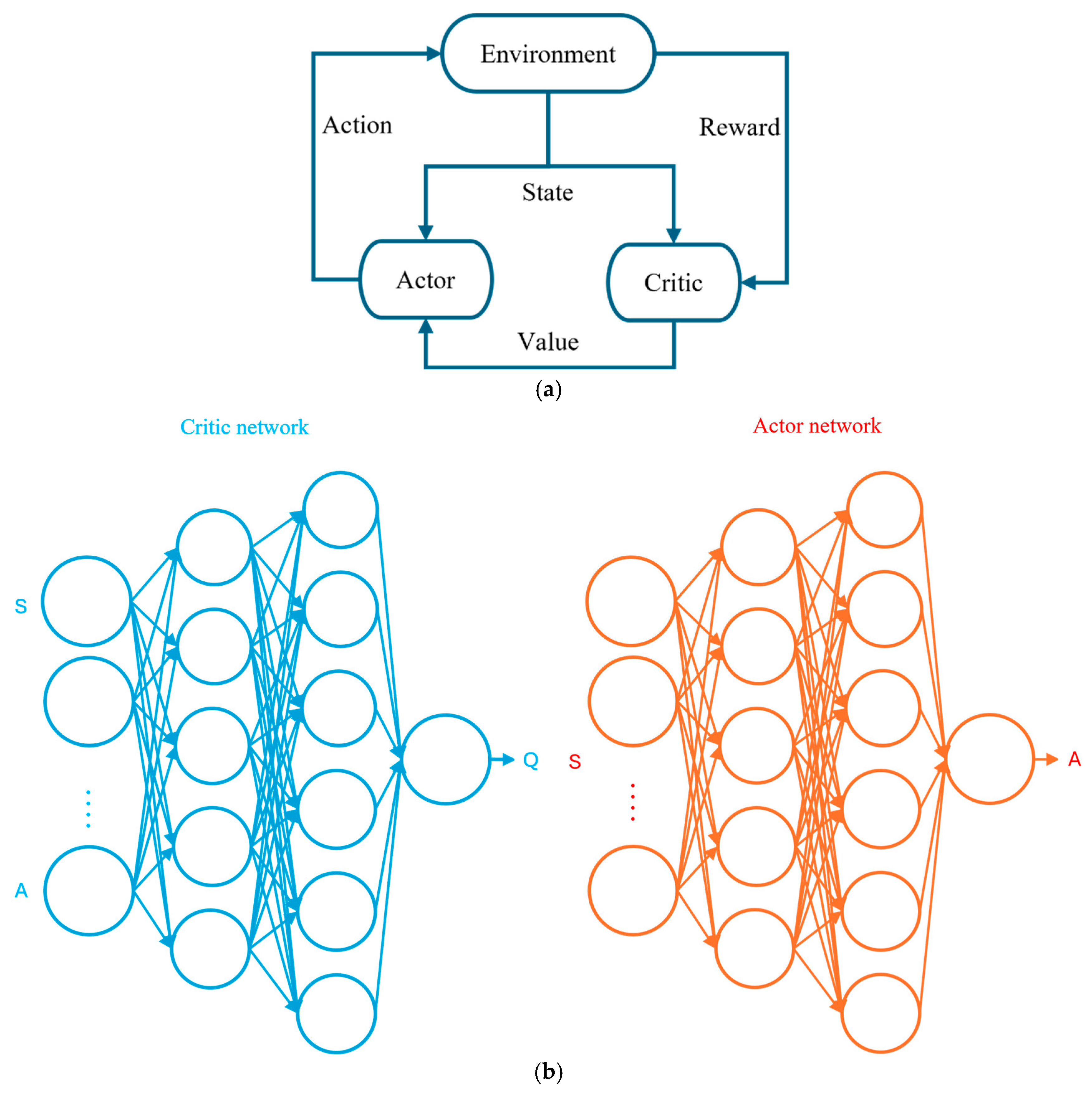
Reinforcement learning is a category of machine learning methods. An agent learns optimal actions through continuous interaction with the environment to maximize long-term cumulative rewards. The reinforcement learning control framework is shown in Figure 2 [39]. In reinforcement learning, problems are typically modeled as a Markov Decision Process (MDP). An MDP consists of the following five fundamental components:
S: State Space. It refers to the setting of all possible environmental states.
A: Action Space. It includes all possible actions that can be taken by the agent.
P: State Transition Probability. It defines the probability of transitioning from a state s t to the next state s t + 1 after taking an action a t . These probabilities depend only on the value of the state s and not on the previous states of the environment [40].
R: Reward Function. It specifies the reward received after taking an action a t in a given state s t .
γ : Discount Factor. It is a value between 0 and 1 that represents the importance of future rewards.
The objective of reinforcement learning is to maximize the cumulative discounted return from the current time step. It is formally expressed as follows:
G t = r t + 1 + γ r t + 2 + γ 2 r t + 3 + = k = 0 γ k r t + k + 1
where G t denotes the return starting from time step t, rt+k represents the reward received at time step t + k, and γ is the discount factor.
The objective of the agent is to learn a policy that selects actions in each state to maximize the long-term cumulative return. Two main approaches are commonly used in reinforcement learning to optimize the policy:
Value-based methods. The policy is optimized indirectly by improving the value function. Common value functions include the state value function V s and the action value function Q s , a . These functions represent the expected return starting from a given state or taking a specific action in each state, respectively:
V π s = E π G t s t = s
Q π s , a = E π G t s t = s , a t = a
The optimal policy corresponds to the optimal state value function V * s and the optimal action value function Q * s , a . These functions represent the maximum expected return that can be achieved by the agent in each state.
Policy-based Methods. The policy is optimized directly by maximizing the expected return. In this approach, the policy π θ a s is parameterized as a function. The agent adjusts the policy parameters θ by computing gradients. The policy gradient theorem provides the direction for policy improvement. Its mathematical expression is given as follows:
θ J θ = E π θ l o g π θ a t s t G t
where J θ denotes the expected return, θ represents the gradient of the parameter θ , and G t represents the return starting from the time step.

2.2.2. Soft Actor–Critic

The core components of SAC include the actor (policy network), the Q-value network (soft Q network), and the critic (value network). These components work together to optimize the policy (see Figure 3). The actor network outputs a probability distribution over actions based on the current state. The Q-value network is used to estimate the value of each state–action pair. The critic network estimates the expected return after taking any action in the current state. The policy is optimized through these components to maximize the cumulative reward.
The core idea of SAC is maximum entropy reinforcement learning. The objective is to maximize the following expected value:
J π = E s t ~ p π , a t ~ π Q π s t , a t α l o g π a t s t
where J π represents the actor’s objective function. The soft Q-value network outputs Q π s t , a t represent the value of selecting an action a t in state s t . The probability distribution π a t s t , output by the policy network, denotes the probability of selecting an action a t in state s t . The temperature parameter α balances the contributions of reward and entropy, controlling the degree of exploration.
The Q-value update in SAC is optimized via the following formula:
L Q = Ε s t , a t ~ Β Q s t , a t r t + γ Ε a t + 1 ~ π Q s t + 1 , a t + 1 α l o g π a t + 1 s t + 1 2
where L Q represents the critic loss function, r t is the immediate reward, γ is the discount factor, and B represents the experience replay buffer containing historical state–action–reward sequences. This formula is designed to optimize the output of the Q-value network by minimizing a loss function. Consequently, the agent is enabled to more accurately estimate the value of state–action pairs.
During policy updates, SAC optimization is performed using the following objective function:
J π = Ε s t ~ ρ π α l o g π a t s t Q π s t , a t
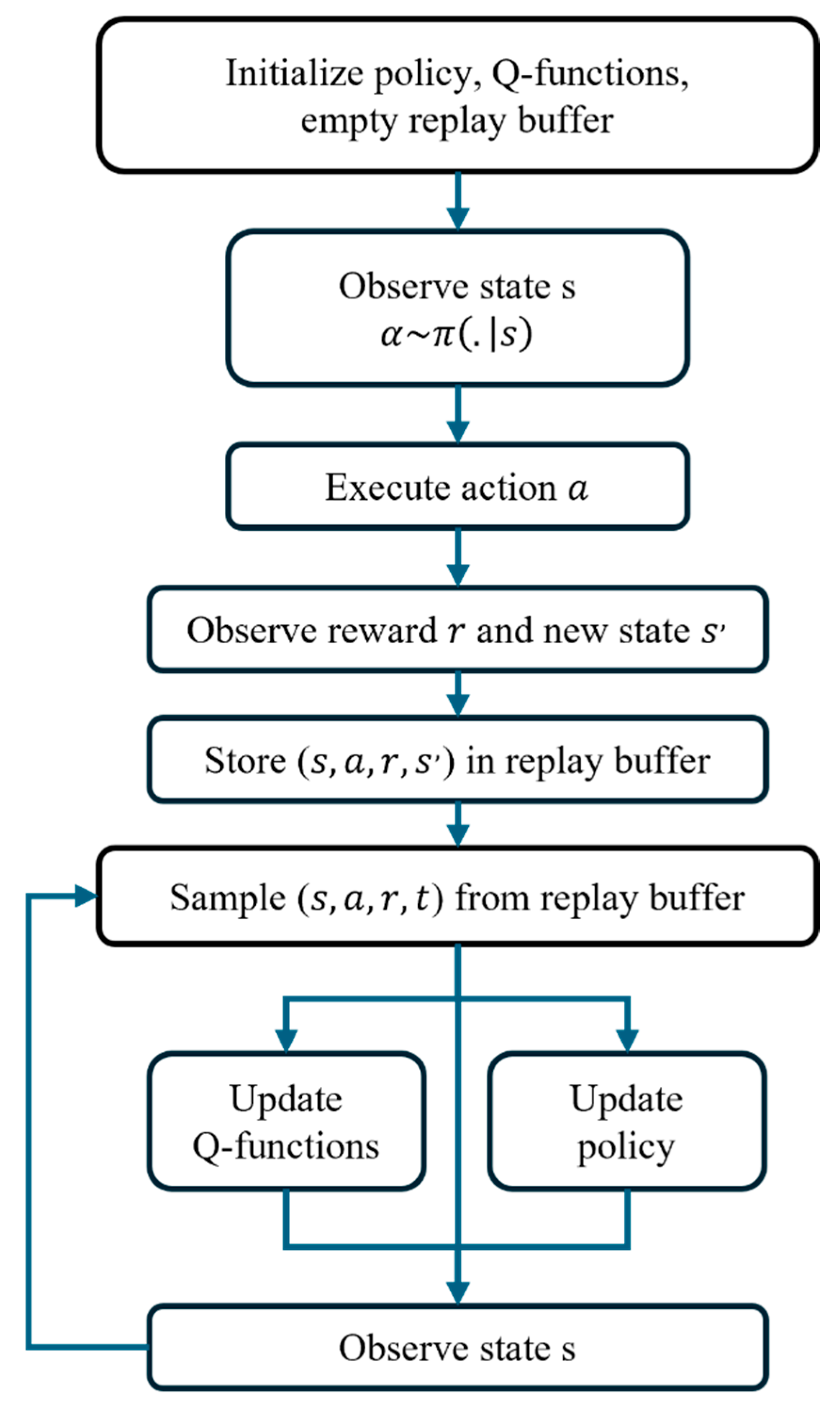
where ρ π represents the state distribution under policy π. By maximizing both the policy entropy and the Q-value, exploration and exploitation are balanced, leading to further policy optimization. For clarity, the main algorithm logic is summarized in Figure 4.

2.2.3. Ordered Replay Buffer

To enhance the stability and convergence efficiency of the SAC algorithm for multi-building collaborative energy management, an improved algorithm named ORAR-SAC is proposed in this study.
The traditional SAC algorithm employs a random experience replay mechanism, uniformly sampling historical interaction data from the experience pool. While this approach helps break temporal correlations between samples, it fails to effectively utilize high-quality experiences, limiting policy convergence speed. Prioritized Experience Replay (PER) commonly quantifies sample learning value through temporal-difference error (TD-error). Higher priority is assigned to samples based on this metric. However, TD-error reflects only value estimation discrepancies. No direct correlation with practical objectives in building scheduling (e.g., electricity load) is established. In contrast, the ORB utilizes a Top K heap structure. High-reward samples are systematically prioritized during replay. As a result, stronger alignment with operational targets such as electricity costs and load profiles is achieved. Consequently, policy optimization is accelerated. When new experiences are added, they are dynamically sorted by reward value. The optimal subset of experiences is retained, enhancing the effectiveness of training data and the efficiency of policy learning.

2.2.4. Alpha Regularization Strategy

In SAC, the temperature parameter α regulates the degree of policy exploration. The temperature is dynamically adjusted based on a target entropy value. Policy entropy is thereby driven toward this predefined target. Exploration–exploitation balance is consequently controlled through entropy regularization. However, control stability remains dependent on appropriate entropy target selection. The target entropy setting directly influences the exploration–exploitation trade-off. To address this limitation, an adaptive temperature optimization mechanism is implemented in ORAR-SAC. When the α value becomes excessively small (indicating over-reliance on exploitation), temperature regularization is activated. Gradient-based adjustments are applied in the reverse direction. Premature policy convergence is thereby effectively prevented.

2.3. Design of DRL Framework and Controller

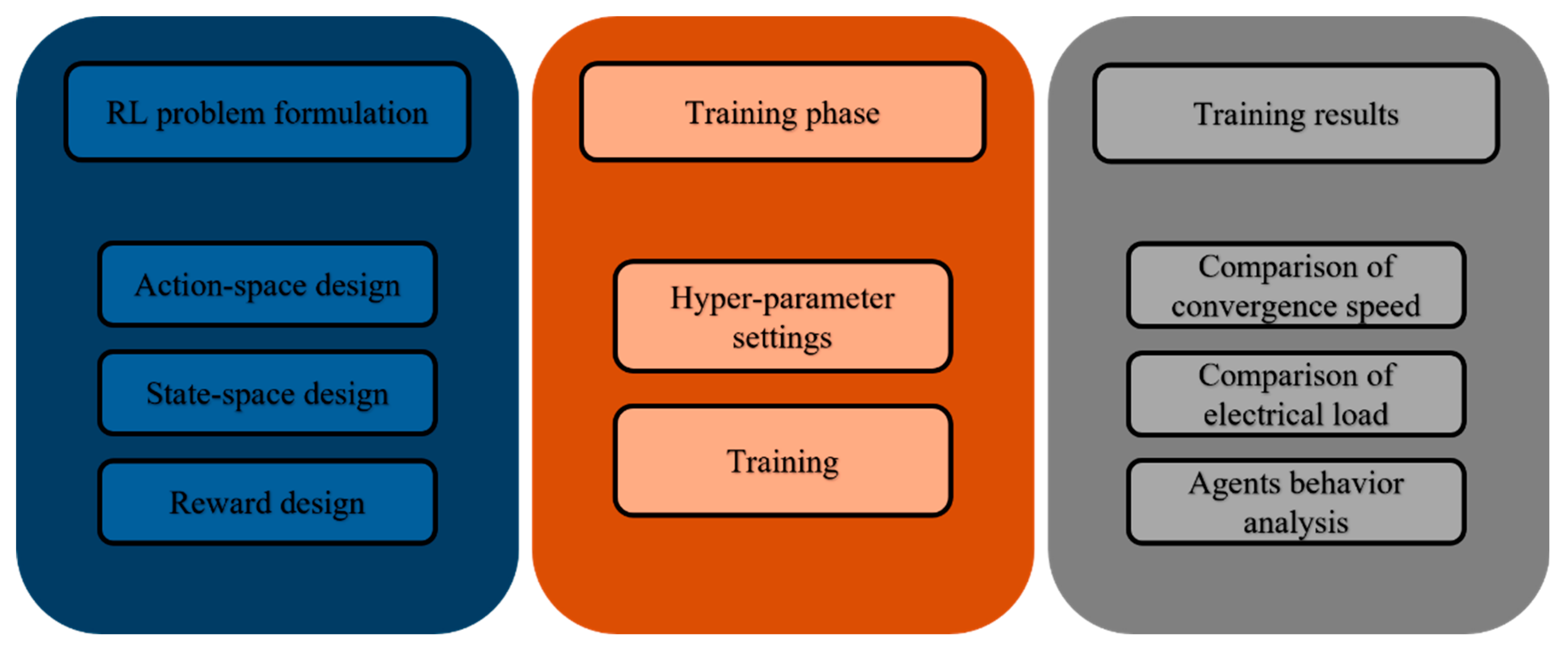
Deep Reinforcement Learning (DRL) control algorithms are employed in this study to optimize the energy management strategies for building clusters. The framework process is specifically illustrated in Figure 5.

2.3.1. Baseline Rule-Based Control

The effectiveness of the DRL controller was evaluated by comparison with an RBC strategy used as the baseline. In the baseline strategy, both cooling and domestic hot water (DHW) energy storage systems were charged during nighttime hours. Charging was evenly distributed throughout the night period. Discharging was uniformly scheduled during daytime hours.
During the initial phase of the SAC algorithm, actions generated by the randomly initialized policy network may exhibit poor performance. To improve early-stage exploration, actions were generated using the RBC strategy. Building load data, simulated using the DeST-C software, served as the raw input data. This approach accelerated early learning, as the RBC strategy provided relatively reasonable actions and reduced ineffective exploration.
Furthermore, the DRL controller was trained based on the RBC strategy. After convergence, the learned policy was compared with the RBC policy. This comparison highlighted the advantages of the DRL controller in multi-building energy management.

2.3.2. Action Space Design

The action space is defined as the set of executable control operations for the agent at each timestep. In this study, the action space for a single building is divided into two control dimensions, corresponding to the charging/discharging rates of the cooling energy storage system and the domestic hot water storage system. Specifically, each action value is normalized to the interval [−0.33, 0.33]. Positive values represent charging, and negative values represent discharging. The value ±1 represents the theoretical maximum rate for a full charge or discharge within 3 h. Actual actions are constrained to within one-third of this value to ensure equipment operational safety and system stability.

2.3.3. State Space Design

The state space represents the agent’s complete observation of the current environment and forms the basis for control policy decisions. In this study, the state space comprises three categories of information, as shown in Table 1.
The state information design is intended to provide the central controller with comprehensive system awareness, enabling both the grasp of overall operational trends and the fine-tuning of local strategies for individual buildings. Figure 6 illustrates the state–action space interaction structure, where the central controller receives mixed state inputs from the building cluster and individual buildings, and outputs dual-action responses for each building.

2.3.4. Reward Design

The reward function serves as the core element of policy optimization, directly determining the behavioral tendencies of the reinforcement learning agent. The reward function designed in this work comprehensively considers both energy consumption costs and peak load. Its specific expression is defined as follows:
R t o t a l = R e c o n o m i c + R s t o r a g e
where R e c o n o m i c represents the economic reward, and R s t o r a g e represents the storage reward. The economic reward is given by:
R e c o n o m i c = B a s e l i n e C o s t C u r r e n t C o s t
In this equation, B a s e l i n e C o s t is defined as the baseline cost. This cost represents the electricity cost incurred by the baseline strategy (RBC) at the same timestep. C u r r e n t C o s t is defined as the actual electricity cost resulting from the agent’s strategy at the current timestep.
The storage reward is expressed as:
R s t o r a g e = i = 1 n ( I 0.2 S O C c o o l i n g i 0.8 * 0.1 + I 0.2 S O C D H W i 0.8 * 0.1 )  
where I denotes the indicator function (equal to 1 if the condition is satisfied, otherwise 0), S O C c o o l i n g i indicates the state of charge (SOC) of the cooling storage device in the i-th building, and S O C D H W i indicates the SOC of the DHW storage device in the i-th building.
In this study, a sensitivity analysis was performed on the storage health incentive weights. Different weight values were tested to control the importance of energy storage health incentives in the overall reward function. The test weight ranged from 0.0 to 1.0, with the specific values listed in Table 2.
The analysis results indicate that the model’s performance is robust to changes in the weights. Even with significant weight changes (e.g., from 0.05 to 0.3), the performance variation was minimal (up to 1.1%). Therefore, the model is not sensitive to different weight values. The sensitivity analysis shows that the impact of energy storage health incentive weights on model performance is minimal, suggesting that the model is not sensitive to changes in this parameter. The current weight setting (0.1) is stable and close to optimal.
A dual-objective fusion mechanism is implemented in this reward function. For the economic objective, a dynamic baseline comparison strategy is adopted. The cost difference between the current strategy and the pre-stored RBC baseline is calculated in real-time. This provides a clear direction for cost optimization. For the equipment health objective, a conditional reward mechanism based on storage SOC is introduced. A constant reward of 0.1 is granted for each cooling or DHW storage unit when its SOC falls within the ideal operating range of 0.2 to 0.8. This design effectively addresses the common “short-sighted optimization” problem in reinforcement learning. Economic benefits are pursued while the safe operation of equipment is simultaneously ensured.

2.3.5. Hyperparameter Design

To ensure training stability and the convergence efficiency of the control policy, the following hyperparameters were optimized during algorithm implementation. All parameters were tuned based on multiple preliminary experiments to achieve a balance between training convergence speed and policy performance. The tested hyperparameters and selected values are summarized in Table 3.
The learning rate is a key hyperparameter in reinforcement learning with moderate sensitivity. A large learning rate can cause unstable training, while a small one can slow down the process. A grid search combined with early stopping was used to test various learning rates, including 0.0005, 0.001, 0.003, 0.01, and 0.03. Based on training stability and convergence speed, 0.001 was selected as the optimal learning rate. The batch size affects training stability and memory usage but has minimal impact on final performance. A batch size of 512, being a power of 2, was chosen to better utilize GPU memory. α, which balances exploration and exploitation, has high sensitivity and directly influences convergence and stability. Various temperature parameter combinations were tested, including [0.5, 0.01], [1.0, 0.05], [1.2, 0.05], and [2.0, 0.1]. The combination [1.2, 0.05] was selected as the final parameters due to its superior performance across different training stages.

2.4. CityLearn Simulation Environment

CityLearn is an open-source simulation environment based on OpenAI Gym, specifically designed for research on multi-building cluster energy management and demand response. The key features of CityLearn include the following:
State and Action Space: The state space covers various building energy efficiency parameters (e.g., temperature, humidity, solar radiation, energy storage system state). The action space primarily consists of adjustments to the charging/discharging of energy storage devices (e.g., batteries, hot water tanks).
Reward Mechanism: Support for user-defined reward functions, typically considering factors such as load smoothness, energy consumption levels, and economic benefits.
Equipment and System Modeling: Built-in models for various energy devices, including photovoltaic generation, battery storage, and hot water storage tanks, enabling dynamic scheduling based on building demands.
In summary, CityLearn provides researchers with a standardized, highly scalable platform, facilitating the testing and comparison of different reinforcement learning algorithms in multi-building cluster energy management.

3. Results

3.1. Study Site

In this study, three commercial buildings located in Beijing were selected for analysis. The building envelope characteristics are shown in Table 4. Each building is equipped with a heat pump to meet cooling demand, an electric heater for DHW demand, and storage systems for both cooling and DHW. For each building, the heat pump is sized to always meet the cooling demand. On the other hand, the storage capacity is designed to be three times the maximum hourly demand for cooling and DHW. In addition, two out of the three buildings are equipped with solar photovoltaic systems. Table 5 shows the main design details of the building energy systems.

3.2. Characteristics of Building Load and Operating Modes

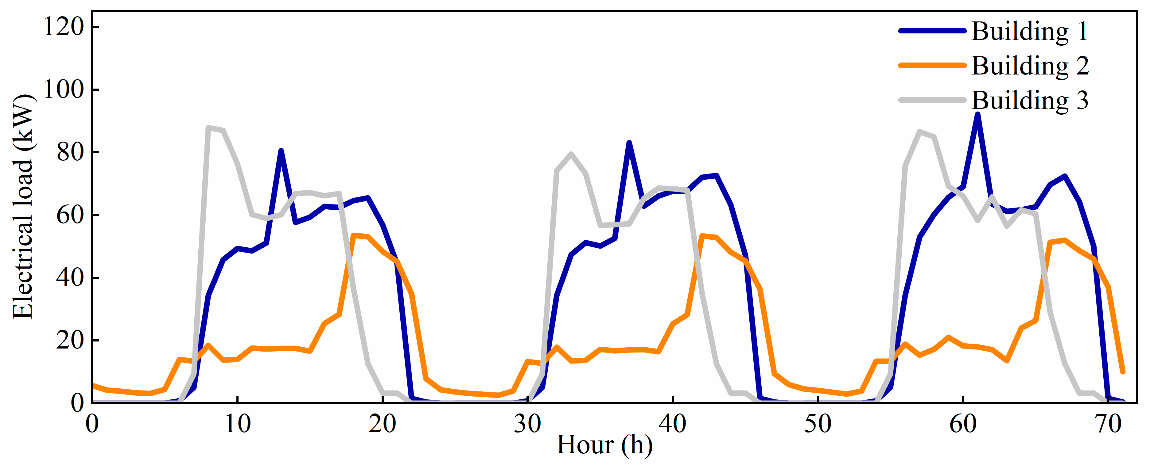
The building loads were simulated using DeST software. Differences in energy consumption among the buildings mainly result from variations in functional types and energy system configurations. This study focuses on the energy consumption characteristics related to cooling and hot water supply during the summer. Cooling demand accounts for a significant portion of the total cluster load. Therefore, only summer performance is considered in the analysis. Figure 7 shows the electricity load curves of each building over three representative summer days. Figure 8 presents the total cluster load along with the photovoltaic generation profile.
The 72 h energy load profiles of the four buildings show significant differences in electricity usage patterns. These differences reflect the influence of functional characteristics and operational modes on energy consumption. Building 1, functioning as a shopping mall, experiences a peak in foot traffic around 1:00 p.m. This results in an increase in the demand for fresh air, leading to a significant rise in ventilation energy consumption. Building 2, functioning as a hotel, experiences a notable increase in guest check-ins around 6:00 p.m., which leads to a surge in electricity demand. Building 3, as an office building, exhibits a high electricity load during working hours (8:00–10:00 and 2:00–5:00 p.m.). The energy cost considered in this study is based on the real-time electricity pricing in Beijing. The specific variation in electricity prices is shown in Figure 9.

3.3. Analysis of Results

3.3.1. Comparative Analysis of Algorithm Convergence

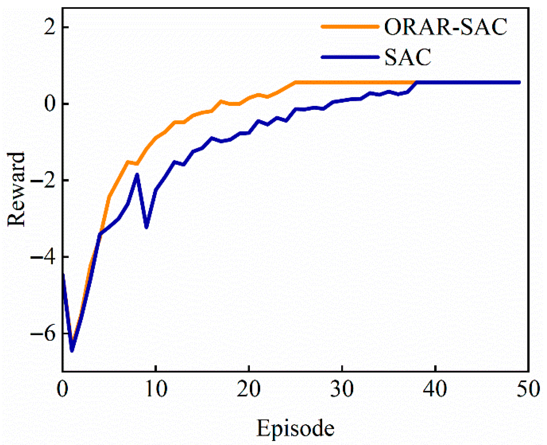
Figure 10 illustrates the convergence performance of the original SAC algorithm and the improved ORAR-SAC algorithm during training. Both algorithms were initialized based on the RBC control policy. Consequently, identical initial rewards were observed. However, as exploration progressed, significant oscillations in rewards were exhibited by the SAC algorithm. In contrast, a smoother convergence curve was demonstrated by the ORAR-SAC algorithm. ORAR-SAC converged at episode 25, while SAC converged at episode 39.
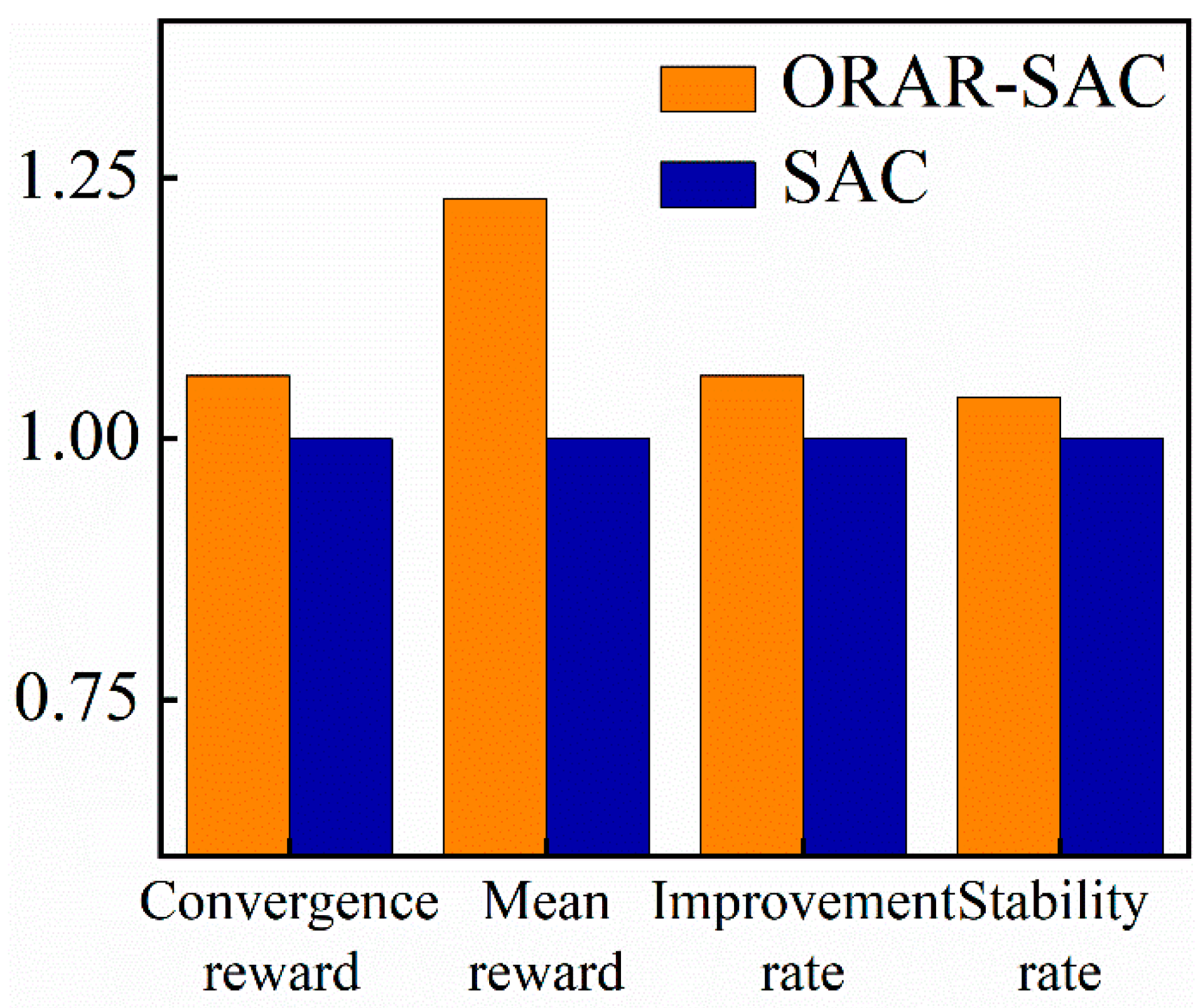
To compare algorithm performance, four metrics were established as evaluation standards: convergence reward, average reward, improvement rate, and stability rate. The SAC algorithm served as the baseline for these comparisons. The normalized comparison results (with SAC set to 1) are presented in Figure 11. Superior performance was shown by the ORAR-SAC algorithm across all four metrics, with increases of 6%, 23%, 6%, and 4%, respectively.
ORAR-SAC achieves a higher average reward than SAC because it improves learning efficiency and stability throughout training, not just at convergence. This leads to a higher average reward overall, even if the final convergence reward difference is smaller. The different proportions between average and convergence reward reflect this training efficiency gap.
This performance improvement is attributed to two key factors. First, the ordered replay buffer prioritized high-value experience samples. Consequently, the policy learning process was accelerated, and training efficiency was significantly enhanced. Second, the exploration–exploitation imbalance was effectively mitigated by the adaptive temperature adjustment mechanism. Stronger exploration intensity was maintained in early training phases, facilitating the discovery of effective policies. Subsequently, exploration intensity was progressively reduced. This approach promoted policy convergence while preventing convergence to local optima.
Overall, ORAR-SAC outperformed the baseline SAC in both convergence speed and training stability, validating the effectiveness of the proposed modifications.

3.3.2. Comparison of Operating Behaviors of Energy Storage Systems

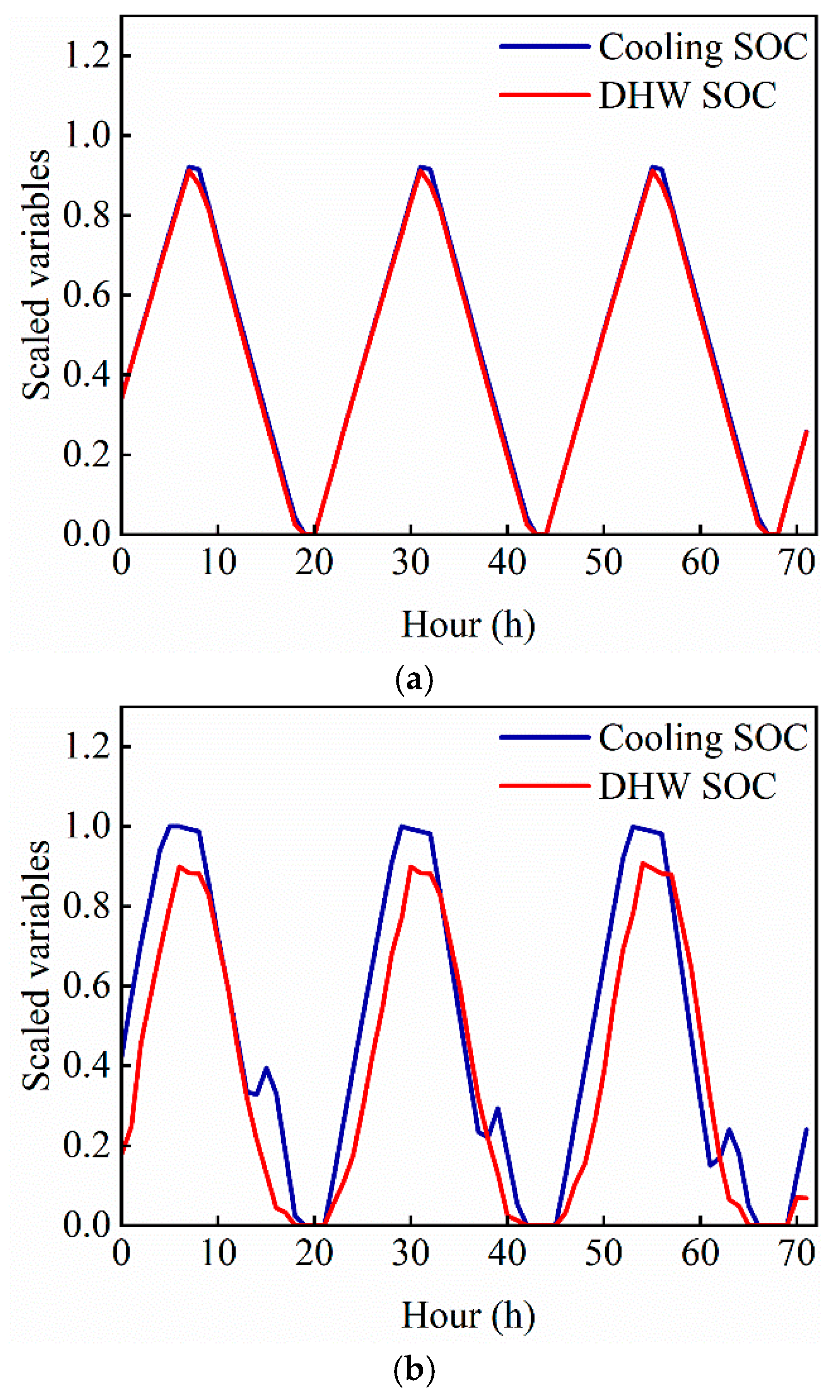
Figure 12 compares the SOC patterns for cooling and DHW storage systems under DRL and RBC strategies. Under the RBC strategy, the storage systems followed a rigid charging/discharging schedule—charging uniformly at night and discharging during the day—regardless of electricity pricing. This led to inefficient energy use and poor responsiveness to pricing signals.
In contrast, the DRL-based controller demonstrated clear periodicity and a strong correlation with the time-of-use price structure. After training based on the RBC baseline, the DRL strategy was able to learn more economical control behaviors. For example, the controller delayed charging until off-peak hours and strategically discharged during peak price periods. Due to the inclusion of SOC-related rewards, the storage systems also initiated moderate charging during mid-price periods in the afternoon, which effectively reduced the cluster’s peak load in the evening. As a result, the DRL strategy enabled more efficient and economical operation, while also producing smoother load profiles.

3.3.3. Comparative Analysis of Building Electrical Load

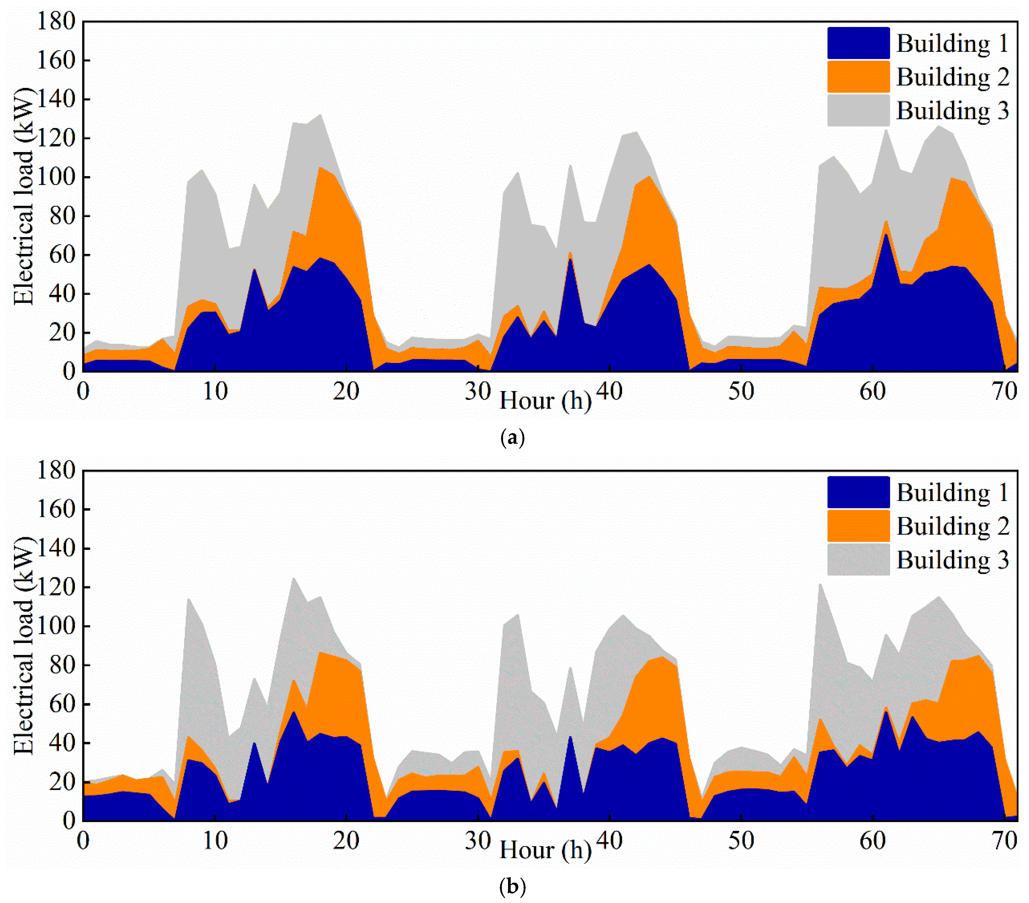
Figure 13 shows the comparison of the building cluster load curves under the RBC and DRL strategies. With ORAR-SAC control, the average peak load was reduced from 126 kW (RBC) to approximately 106 kW. The number of sharp load peaks was significantly reduced, and the overall profile became smoother, thereby alleviating stress on the power grid. During off-peak periods, the DRL-controlled load stabilized around 35 kW, compared to below 20 kW under RBC. This improvement was due to the DRL controller’s ability to learn electricity price patterns and schedule storage systems accordingly, achieving effective load shifting and peak shaving.
Furthermore, under ORAR-SAC, daytime loads were noticeably lower than those under RBC, as the controller actively discharged storage to suppress demand during high-price hours. Through coordinated scheduling across multiple buildings, the DRL controller distributed loads more evenly, reducing overall system stress and improving both operational stability and cost efficiency.
In summary, the DRL control strategy effectively captured electricity pricing signals and load distribution features. By enabling adaptive scheduling, it successfully achieved the dual objectives of load leveling and cost optimization. The control performance significantly surpassed that of the traditional rule-based strategy.
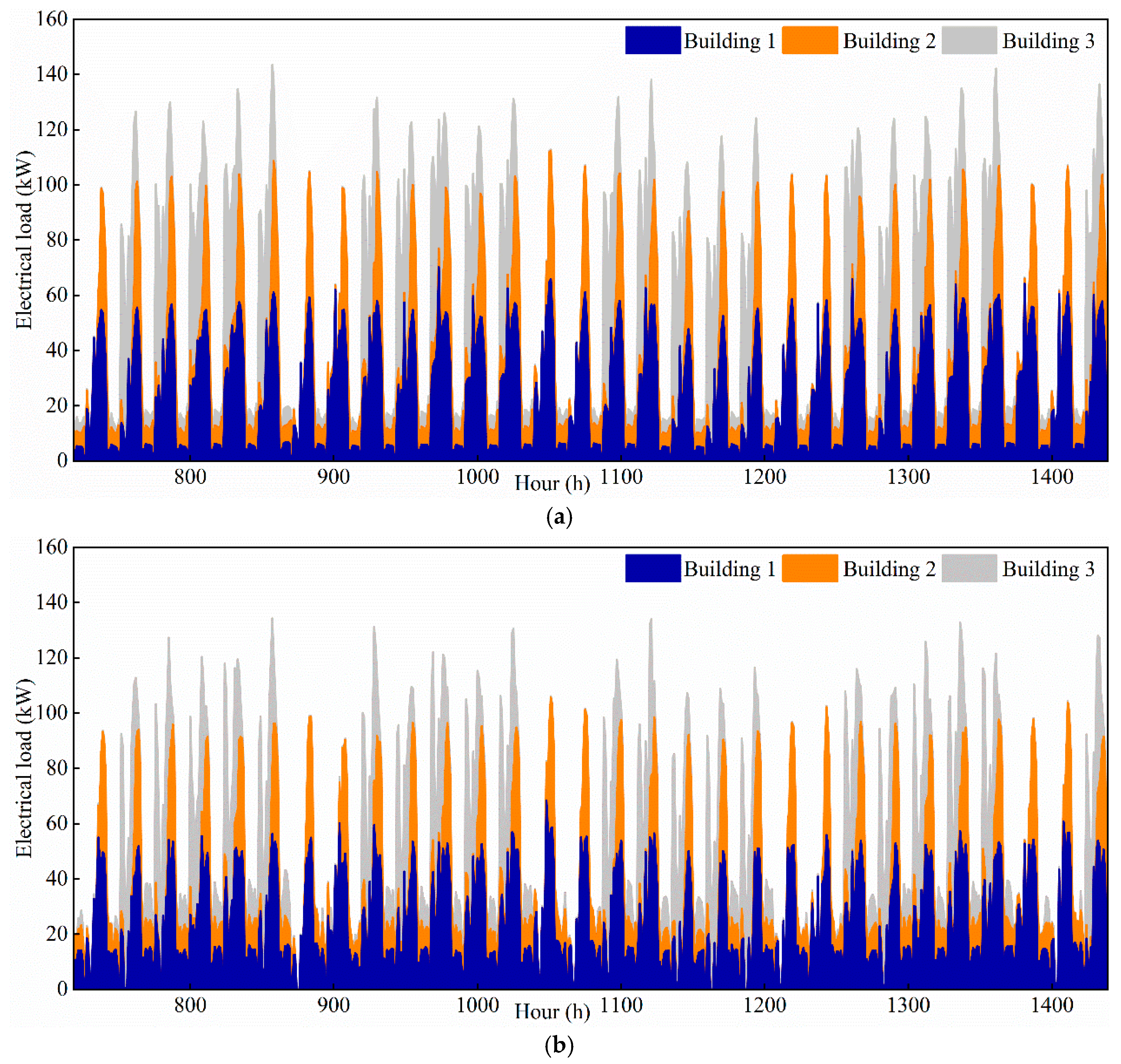
The stability and generalization capability of the DRL control strategy were evaluated. Figure 14 presents a comparison of the building cluster load profiles under the RBC and ORAR-SAC strategies over a continuous 30-day operation. Under the ORAR-SAC strategy, the monthly peak load was reduced from 143 kW to 123 kW. The average daily peak load also decreased, from 121 kW to 114 kW. These reductions demonstrate the strategy’s sustained ability to smooth load peaks. Conversely, the average daily load during valley periods within the month increased from 17 kW to 28 kW. This increase highlights the long-term consistency of the energy storage system scheduling strategy. The simulation spanned 30 consecutive days. This duration covered multiple weekdays and weekends. Diverse building load demands were presented during this period. Consequently, complex and dynamic operating conditions were provided by the controller. Under these conditions, smooth load profiles were consistently maintained by the DRL controller. Peak loads were significantly suppressed. Furthermore, no abnormal oscillations or runaway behavior were observed. These results indicate strong stability of the proposed controller.

3.3.4. Quantitative Comparison of Key Performance Indicators (KPIs)

To quantitatively evaluate the performance differences, several KPIs were defined, including total energy consumption, total electricity cost, carbon emissions, peak load, and average daily peak load (presented in Table 6). At the cluster level, the DRL strategy achieved a 3.5% reduction in energy consumption, 11% savings in electricity cost, 3.5% decrease in carbon emissions, 7% reduction in peak load, and a 10% decrease in average daily peak load. To ensure reproducibility and statistical significance, 10 random seeds were selected for model initialization. The results were analyzed across three metrics: electricity consumption, electricity cost, and peak load (see in Table 7). For each metric, p-values below 0.05 were observed. These findings indicate statistically significant differences.
These improvements reflect not only enhanced energy balancing but also demonstrate the practical value of DRL in optimizing the interaction between building clusters and the power grid.

4. Discussion

This study proposes and validates a model-free DRL control strategy—ORAR-SAC—for coordinated energy management in building clusters, implemented within the CityLearn simulation platform. The objective is to minimize both electricity costs and peak demand by scheduling the charge and discharge behavior of energy storage systems under a time-of-use electricity pricing scheme representative of Beijing.
To evaluate the effectiveness of the proposed DRL controller and highlight the benefits of cluster-level coordination over single-building optimization, a traditional RBC strategy was adopted as a baseline for systematic comparison.
Given the challenges of applying the standard SAC algorithm in complex environments such as building clusters, two key mechanisms were introduced: the Ordered Replay Buffer and the Alpha Regularization Strategy. The former improves sample efficiency and accelerates policy convergence by prioritizing high-value experience samples, while the latter regulates exploration by dynamically adjusting the temperature parameter α, thereby enhancing training stability and preventing policy oscillations. These improvements were validated through convergence curve analysis, demonstrating that the proposed method achieves a balance between training efficiency and control robustness.
Despite the complexity of the environment, the DRL controller was able to learn optimal scheduling behaviors. This enabled more efficient energy use and better alignment of storage operations with real-time system demands, thereby flattening the cluster-level load profile.

5. Conclusions

The study simulated summer operation scenarios for a cluster composed of three buildings with distinct functional attributes: a shopping mall, a hotel, and an office building. Results show that the RBC strategy exhibited delayed responsiveness and low energy-shifting efficiency in managing cooling and DHW storage. Its operations did not adapt to electricity price fluctuations, resulting in either excessive or insufficient utilization of storage capacity.
In contrast, the ORAR-SAC controller exhibited clear periodic patterns and strong responsiveness to the electricity pricing structure. Charging activities were concentrated during off-peak hours, while discharging occurred during peak periods. This behavior reflects the controller’s ability to learn economic scheduling policies.
At the cluster level, ORAR-SAC achieved a 3.5% reduction in total energy consumption, an 11% decrease in electricity costs, a 3.5% reduction in carbon emissions, and a 7% decrease in peak demand compared to the RBC strategy. The system also exhibited smoother operation and improved grid compatibility, indicating strong potential for real-world deployment.
Future research may consider several directions: (1) extending the framework to winter conditions, where centralized heating systems such as gas-fired boilers are commonly used, to assess seasonal performance differences and improve the adaptability of the proposed method; (2) developing decoupled control strategies tailored to diverse building loads; (3) incorporating transfer learning and online adaptation to improve robustness under dynamic conditions; (4) integrating real building operational data and user behavior models to increase practical relevance; and (5) exploring multi-agent reinforcement learning (MARL) frameworks to achieve decentralized coordination among buildings and enhance scalability.
In conclusion, ORAR-SAC, which combines reinforcement learning with structural optimization strategies, demonstrates significant advantages in multi-building energy management. It offers a promising technical pathway for intelligent building operation and the development of low-carbon cities.

Author Contributions

Conceptualization, W.L. and Y.G.; methodology, W.L. and Z.S.; software, W.L.; validation, W.L.; formal analysis, W.L.; data curation, Q.M.; writing—original draft preparation, W.L.; writing—review and editing, W.L. and Z.S.; visualization, W.L.; supervision, Y.G. All authors have read and agreed to the published version of the manuscript.

Funding

This research received no external funding.

Institutional Review Board Statement

Not applicable.

Informed Consent Statement

Not applicable.

Data Availability Statement

The original contributions presented in this study are included in the article. Further inquiries can be directed to the corresponding author.

Conflicts of Interest

The authors declare no conflicts of interest.

Abbreviations

The following abbreviations are used in this manuscript:
SACSoft Actor–Critic
ORAR-SACOrdered replay and Alpha regularization Soft Actor–Critic
ACAir conditioning
RBCRule-Based Control
MPCModel Predictive Control
RLReinforcement learning
PVPhotovoltaic
MDPMarkov Decision Process
DRLDeep Reinforcement Learning
DHWDemand heating water
KPIKey performance indicator

References

  1. Gupta, V.; Deb, C. Envelope design for low-energy buildings in the tropics: A review. Renew. Sustain. Energy Rev. 2023, 186, 113650. [Google Scholar] [CrossRef]
  2. Li, S.; Li, Y.; Wang, M.; Peng, J.; He, Y. Optimization study of photovoltaic direct-driven air conditioning system based on occupants’ behavior and thermal comfort. Renew. Energy 2025, 251, 123389. [Google Scholar] [CrossRef]
  3. Sun, Z.; Gao, Y.; Yang, J.; Chen, Y.; Guo, B.H.W. Development of urban building energy models for Wellington city in New Zealand with detailed survey data on envelope thermal characteristics. Energy Build. 2024, 321, 114647. [Google Scholar] [CrossRef]
  4. Blad, C.; Bøgh, S.; Kallesøe, C. A Multi-Agent Reinforcement Learning Approach to Price and Comfort Optimization in HVAC-Systems. Energies 2021, 14, 7491. [Google Scholar] [CrossRef]
  5. Gao, Y.; Sun, Z.; Lin, X.; Wang, C.; Sun, Z.; Chen, Y. Designing and Optimizing Heat Storage of a Solar-Assisted Ground Source Heat Pump System in China. Int. J. Photoenergy 2020, 2020, 1–18. [Google Scholar] [CrossRef]
  6. Siano, P. Demand response and smart grids—A survey. Renew. Sustain. Energy Rev. 2014, 30, 461–478. [Google Scholar] [CrossRef]
  7. Battaglia, M.; Haberl, R.; Bamberger, E.; Haller, M. Increased self-consumption and grid flexibility of PV and heat pump systems with thermal and electrical storage. Energy Procedia 2017, 135, 358–366. [Google Scholar] [CrossRef]
  8. Sun, L.; Li, J.; Chen, L.; Xi, J.; Li, B. Energy storage capacity configuration of building integrated photovoltaic-phase change material system considering demand response. IET Energy Syst. Integr. 2021, 3, 263–272. [Google Scholar] [CrossRef]
  9. Nematirad, R.; Pahwa, A.; Natarajan, B.; Wu, H. Optimal sizing of photovoltaic-battery system for peak demand reduction using statistical models. Front. Energy Res. 2023, 11, 1297356. [Google Scholar] [CrossRef]
  10. Rashid, M.M.U.; Granelli, F.; Hossain, M.A.; Alam, M.S.; Al-Ismail, F.S.; Shah, R. Development of Cluster-Based Energy Management Scheme for Residential Usages in the Smart Grid Community. Electronics 2020, 9, 1462. [Google Scholar] [CrossRef]
  11. Gonzato, S.; Chimento, J.; O’Dwyer, E.; Bustos-Turu, G.; Acha, S.; Shah, N. Hierarchical price coordination of heat pumps in a building network controlled using model predictive control. Energy Build. 2019, 202, 109421. [Google Scholar] [CrossRef]
  12. Manrique Delgado, B.; Ruusu, R.; Hasan, A.; Kilpeläinen, S.; Cao, S.; Sirén, K. Energetic, Cost, and Comfort Performance of a Nearly-Zero Energy Building Including Rule-Based Control of Four Sources of Energy Flexibility. Buildings 2018, 8, 172. [Google Scholar] [CrossRef]
  13. Zou, B.; Peng, J.; Li, S.; Li, Y.; Yan, J.; Yang, H. Comparative study of the dynamic programming-based and rule-based operation strategies for grid-connected PV-battery systems of office buildings. Appl. Energy 2022, 305, 117875. [Google Scholar] [CrossRef]
  14. Afram, A.; Janabi-Sharifi, F.; Fung, A.S.; Raahemifar, K. Artificial neural network (ANN) based model predictive control (MPC) and optimization of HVAC systems: A state of the art review and case study of a residential HVAC system. Energy Build. 2017, 141, 96–113. [Google Scholar] [CrossRef]
  15. Schwenzer, M.; Ay, M.; Bergs, T.; Abel, D. Review on model predictive control: An engineering perspective. Int. J. Adv. Manuf. Technol. 2021, 117, 1327–1349. [Google Scholar] [CrossRef]
  16. El Makroum, R.; Khallaayoun, A.; Lghoul, R.; Mehta, K.; Zörner, W. Home Energy Management System Based on Genetic Algorithm for Load Scheduling: A Case Study Based on Real Life Consumption Data. Energies 2023, 16, 2698. [Google Scholar] [CrossRef]
  17. Malik, S.; Kim, D. Prediction-Learning Algorithm for Efficient Energy Consumption in Smart Buildings Based on Particle Regeneration and Velocity Boost in Particle Swarm Optimization Neural Networks. Energies 2018, 11, 1289. [Google Scholar] [CrossRef]
  18. Rajwar, K.; Deep, K.; Das, S. An exhaustive review of the metaheuristic algorithms for search and optimization: Taxonomy, applications, and open challenges. Artif. Intell. Rev. 2023, 56, 13187–13257. [Google Scholar] [CrossRef]
  19. Manjavacas, A.; Campoy-Nieves, A.; Jiménez-Raboso, J.; Molina-Solana, M.; Gómez-Romero, J. An experimental evaluation of deep reinforcement learning algorithms for HVAC control. Artif. Intell. Rev. 2024, 57, 173. [Google Scholar] [CrossRef]
  20. Wei, T.; Wang, Y.; Zhu, Q. Deep Reinforcement Learning for Building HVAC Control. In Proceedings of the 54th Annual Design Automation Conference, Austin, TX, USA, 18–22 June 2017; ACM: New York, NY, USA, 2017; pp. 1–6. [Google Scholar]
  21. Vázquez-Canteli, J.R.; Nagy, Z. Reinforcement learning for demand response: A review of algorithms and modeling techniques. Appl. Energy 2019, 235, 1072–1089. [Google Scholar] [CrossRef]
  22. Brandi, S.; Piscitelli, M.S.; Martellacci, M.; Capozzoli, A. Deep reinforcement learning to optimise indoor temperature control and heating energy consumption in buildings. Energy Build. 2020, 224, 110225. [Google Scholar] [CrossRef]
  23. Wang, Z.; Hong, T. Reinforcement learning for building controls: The opportunities and challenges. Appl. Energy 2020, 269, 115036. [Google Scholar] [CrossRef]
  24. Ruelens, F.; Claessens, B.J.; Vandael, S.; De Schutter, B.; Babuska, R.; Belmans, R. Residential Demand Response of Thermostatically Controlled Loads Using Batch Reinforcement Learning. IEEE Trans. Smart Grid 2017, 8, 2149–2159. [Google Scholar] [CrossRef]
  25. Lu, R.; Hong, S.H. Incentive-based demand response for smart grid with reinforcement learning and deep neural network. Appl. Energy 2019, 236, 937–949. [Google Scholar] [CrossRef]
  26. Kazmi, H.; Mehmood, F.; Lodeweyckx, S.; Driesen, J. Gigawatt-hour scale savings on a budget of zero: Deep reinforcement learning based optimal control of hot water systems. Energy 2018, 144, 159–168. [Google Scholar] [CrossRef]
  27. Fang, P.; Wang, M.; Li, J.; Zhao, Q.; Zheng, X.; Gao, H. A Distributed Intelligent Lighting Control System Based on Deep Reinforcement Learning. Appl. Sci. 2023, 13, 9057. [Google Scholar] [CrossRef]
  28. Avila, L.; De Paula, M.; Trimboli, M.; Carlucho, I. Deep reinforcement learning approach for MPPT control of partially shaded PV systems in Smart Grids. Appl. Soft Comput. 2020, 97, 106711. [Google Scholar] [CrossRef]
  29. Phan, B.C.; Lai, Y.-C.; Lin, C.E. A Deep Reinforcement Learning-Based MPPT Control for PV Systems under Partial Shading Condition. Sensors 2020, 20, 3039. [Google Scholar] [CrossRef] [PubMed]
  30. Fu, Y.; Ren, Z.; Wei, S.; Huang, L.; Li, F.; Liu, Y. Dynamic Optimal Power Flow Method Based on Reinforcement Learning for Offshore Wind Farms Considering Multiple Points of Common Coupling. J. Mod. Power Syst. Clean Energy 2024, 12, 1749–1759. [Google Scholar] [CrossRef]
  31. Darbandi, A.; Brockmann, G.; Ni, S.; Kriegel, M. Energy scheduling strategy for energy hubs using reinforcement learning approach. J. Build. Eng. 2024, 98, 111030. [Google Scholar] [CrossRef]
  32. Sun, H.; Hu, Y.; Luo, J.; Guo, Q.; Zhao, J. Enhancing HVAC Control Systems Using a Steady Soft Actor–Critic Deep Reinforcement Learning Approach. Buildings 2025, 15, 644. [Google Scholar] [CrossRef]
  33. Park, Y.; Jun, W.; Lee, S. A Comparative Study of Deep Reinforcement Learning Algorithms for Urban Autonomous Driving: Addressing the Geographic and Regulatory Challenges in CARLA. Appl. Sci. 2025, 15, 6838. [Google Scholar] [CrossRef]
  34. Zhao, Y.; Lin, F.; Yang, Z. Soft Actor-Critic-Based Energy Management Strategy for Hybrid Energy Storage System in Urban Rail Transit Dc Traction Power Supply System. Elsevier BV 2025. [Google Scholar] [CrossRef]
  35. Li, H.; Qian, X.; Song, W. Prioritized experience replay based on dynamics priority. Sci. Rep. 2024, 14, 6014. [Google Scholar] [CrossRef]
  36. Zhang, Z.; Fu, H.; Yang, J.; Lin, Y. Deep reinforcement learning for path planning of autonomous mobile robots in complicated environments. Complex Intell. Syst. 2025, 11, 277. [Google Scholar] [CrossRef]
  37. Kaspar, K.; Nweye, K.; Buscemi, G.; Capozzoli, A.; Nagy, Z.; Pinto, G.; Eicker, U.; Ouf, M.M. Effects of occupant thermostat preferences and override behavior on residential demand response in CityLearn. Energy Build. 2024, 324, 114830. [Google Scholar] [CrossRef]
  38. Yan, D.; Zhou, X.; An, J.; Kang, X.; Bu, F.; Chen, Y.; Pan, Y.; Gao, Y.; Zhang, Q.; Zhou, H.; et al. DeST 3.0: A new-generation building performance simulation platform. Build. Simul. 2022, 15, 1849–1868. Available online: https://link.springer.com/article/10.1007/s12273-022-0909-9 (accessed on 2 July 2025). [CrossRef]
  39. Yatawatta, S. Reinforcement learning. Astron. Comput. 2024, 48, 100833. [Google Scholar] [CrossRef]
  40. Han, M.; May, R.; Zhang, X.; Wang, X.; Pan, S.; Yan, D.; Jin, Y.; Xu, L. A review of reinforcement learning methodologies for controlling occupant comfort in buildings. Sustain. Cities Soc. 2019, 51, 101748. [Google Scholar] [CrossRef]
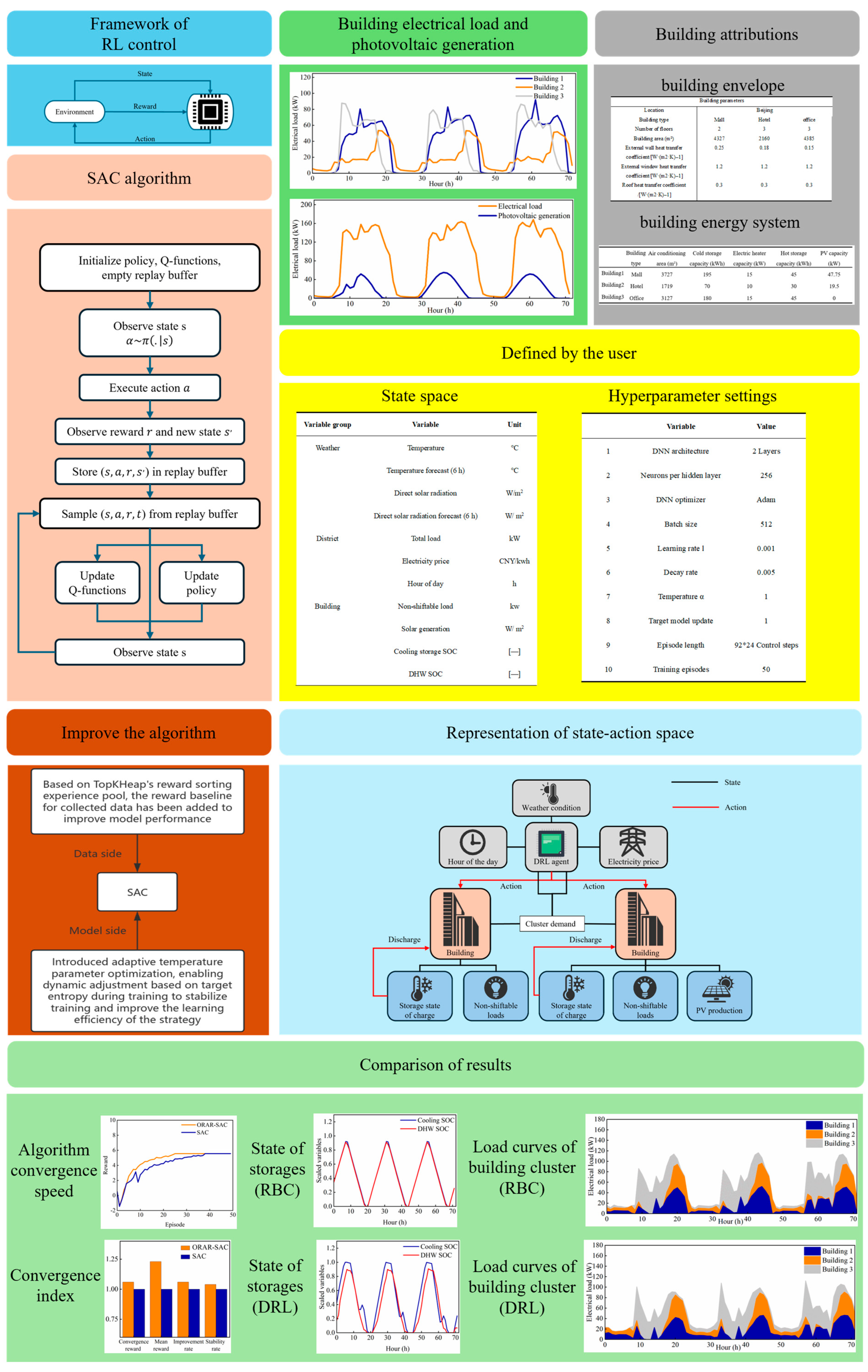
Figure 1. Framework of DRL for optimizing energy management in the building cluster.
Applsci 15 08966 g001
Figure 2. Reinforcement learning control framework.
Applsci 15 08966 g002
Figure 3. Actor–Critic–Environment interaction and neural networks in DRL. (a) Actor–Critic–Environment interaction. (b) Neural networks.
Applsci 15 08966 g003
Figure 4. Soft Actor–Critic algorithm.
Applsci 15 08966 g004
Figure 5. Framework of the application of DRL control.
Applsci 15 08966 g005
Figure 6. Representation of the state–action space.
Applsci 15 08966 g006
Figure 7. Electricity load of individual buildings.
Applsci 15 08966 g007
Figure 8. Electrical load and photovoltaic generation of the building cluster.
Applsci 15 08966 g008
Figure 9. Electricity price.
Applsci 15 08966 g009
Figure 10. Comparison of algorithm convergence curves.
Applsci 15 08966 g010
Figure 11. Comparison of algorithm performance.
Applsci 15 08966 g011
Figure 12. SOC of energy storage devices under different strategies. (a) RBC control strategy. (b) DRL control strategy.
Applsci 15 08966 g012
Figure 13. Load curves of the building cluster under different strategies. (a) Load curves of the building cluster (RBC). (b) Load curves of the building cluster (DRL).
Applsci 15 08966 g013
Figure 14. Load curve of the building cluster under different strategies within 30 days. (a) Load curves of the building cluster (RBC). (b) Load curves of the building cluster (DRL).
Applsci 15 08966 g014
Table 1. Categories of information in the state space.
Variable GroupVariableUnit
WeatherTemperature°C
Temperature forecast (6 h)°C
Direct solar radiationW/m2
Direct solar radiation forecast (6 h)W/m2
DistrictTotal loadkW
Electricity priceCNY/kWh
Hour of dayH
BuildingNon-shiftable loadkW
Solar generationW/m2
Cooling storage SOC[—]
DHW SOC[—]
Table 2. Sensitivity analysis of storing health incentive weights.
Weight ValueAverage RewardRelative
Performance
0.05−2702.580.00%
0.08−2698.080.00%
0.1−2695.080.00%
0.12−2698.08−0.11%
0.15−2702.58−0.28%
0.2−2710.08−0.55%
0.3−2725.08−1.10%
Table 3. Summary of hyperparameters.
VariableValue
1DNN architecture2 Layers
2Neurons per hidden layer256
3DNN optimizerAdam
4Batch size512
5Learning rate l0.001
6Decay rate0.005
7Temperature α1.2
8Target model update2
9Episode length92 * 24 Control steps
10Training episodes50
Table 4. Building envelope structure.
Building Parameters
LocationBeijing
Building typeMallHoteloffice
Number of floors233
Building area (m2)432721604385
External wall heat transfer coefficient/[W·(m2·K)−1]0.250.180.15
External window heat transfer coefficient/[W·(m2·K)−1]1.21.21.2
Roof heat transfer coefficient
/[W·(m2·K)−1]
0.30.30.3
Table 5. Energy systems properties.
Building TypeAir Conditioning Area (m2)Cold Storage Capacity (kWh)Electric Heater Capacity (kW)Hot Storage Capacity (kWh)PV Capacity (kW)
Building1Mall3727195154547.75
Building2Hotel171970103019.5
Building3Office312718015450
Table 6. Comparison performance of the two control strategies.
Energy
Consumption/kWh
Electricity
Cost/CNY
Carbon
Emissions/
kg CO2
Peak Load/kWAverage Daily
Peak Load/kW
ORAR-SAC113,103106,83363,111148105
RBC117,155120,29865,372159117
Table 7. Significant statistics.
Energy
Consumption/kWh
p-ValueElectricity
Cost/CNY
p-ValuePeak Load/kWp-Value
ORAR-SAC113,133 ± 326 8 × 10 6 106,982 ±   358 7.4 × 10 5 146 ± 4 6.2 × 10 5
RBC117,203 ±   109 120,348 ±   176 160 ± 2
Disclaimer/Publisher’s Note: The statements, opinions and data contained in all publications are solely those of the individual author(s) and contributor(s) and not of MDPI and/or the editor(s). MDPI and/or the editor(s) disclaim responsibility for any injury to people or property resulting from any ideas, methods, instructions or products referred to in the content.