Node Embedding and Cosine Similarity for Efficient Maximum Common Subgraph Discovery

Abstract

Finding the maximum common induced subgraph is a fundamental problem in computer science. Proven to be NP-hard in the 1970s, it has, nowadays, countless applications that still motivate the search for efficient algorithms and practical heuristics. In this work, we extend a state-of-the-art branch-and-bound exact algorithm with new techniques developed in the deep-learning domain, namely graph neural networks and node embeddings, effectively transforming an efficient yet uninformed depth-first search into an effective best-first search. The change enables the algorithm to find suitable solutions within a limited budget, pushing forward the method’s time efficiency and applicability on larger graphs. We evaluate the usage of the L2 norm of the node embeddings and the Cumulative Cosine Similarity to classify the nodes of the graphs. Our experimental analysis on standard graphs compares our heuristic against the original algorithm and a recently tweaked version that exploits reinforcement learning. The results demonstrate the effectiveness and scalability of the proposed approach, compared with the state-of-the-art algorithms. In particular, this approach results in improved results on over 90% of the larger graphs; this would be more challenging in a constrained industrial scenario.

1. Introduction

Graphs are extremely general and consequential data structures. Programmers can use them to model, analyze, and process various phenomena and concepts by providing natural, machine-readable representations [1]. They model many elements of human knowledge through a mathematical abstraction. In particular, graphs can be excellent representations of relationships between objects and are incredibly versatile, showing up in various fields. For instance, they are crucial in chemistry [2] for understanding molecular structures, in analyzing social networks [3] to reveal connections, and in powering web searches [4] like Google’s PageRank algorithm. You will also find them in security threat detection [5], in modeling dependencies between software components [6], and even in hardware testing and functional test programs [7].

The Maximum Common Subgraph (MCS) problem consists of finding the most extensive graph isomorphic to a subgraph of two given graphs [8,9]. In the specialized literature, this problem comes in the induced and partial forms. In the former, we find a graph with as many vertices as possible, in which we map edges to edges and non-edges to non-edges. In the latter, we find a subgraph with the maximum number of edges. In the following, we will tackle the most common variant, the induced one, and we shall denote it simply as the MCS problem, as in many scientific works.

1.1. Related Works

The MCS problem remains an active area of research due to its computational intractability and broad applicability. Researchers have presented algorithms to find the MCS in the literature since the seventies [8,9]. Among the less recent notable algorithms, we may recall conversions to the Maximum Common Clique problem [10], integer linear programming [11], and constraint programming [12,13]. Conversely, more recent efforts have focused on improving exact solvers or estimation heuristics, exploring novel approaches like machine learning [14,15] and quantum computing, or facing the problem of trying different perspectives (like graph simplification) [16,17]. Regarding the work related to our approach, we describe the following in more detail.

Barrow et al. [9] propose solving the subgraph isomorphism problem by transforming it into a maximal clique problem in a specially constructed “association graph.” The core idea is that if graph G is isomorphic to a subgraph of graph H, then a clique of a specific size exists in the product graph. One main contribution is the transformation method to convert subgraph isomorphism into a maximal clique problem. It is unlikely that the constructed product graph can become very large, and the transformation does not fundamentally change the NP-complete inherent complexity of the problem.

Guidobene et al. [18] introduce new heuristics for the MCS problem by reformulating it as the Maximum Clique Problem and its complement, the Maximum Independent Set. The authors apply heuristics for the Maximum Independent Set problem to efficiently reduce graph sizes, enabling faster computation. Unfortunately, the proposed heuristics aim for near-optimal solutions, implying they might not always find the exact maximum common subgraph. Moreover, the authors tested primarily on randomly generated Erdös–R‘enyi graph pairs, which may not fully represent the diversity and complexity of real-world graphs. Finally, they rely on local optima convergence, which might still become stuck in suboptimal solutions depending on the initialization and annealing schedule.

Yu et al. [19] introduce RRSplit, a new backtracking algorithm aimed at improving practical efficiency and providing theoretical guarantees on worst-case running times. The algorithm leverages new reduction techniques and refined upper bounds to minimize redundant computations during the search. Unfortunately, the theoretical guarantees may still indicate high complexity for extremely large or dense graphs, given the NP-hard nature of MCS. Moreover, the complexity of implementing the new reductions and upper bounds might be higher than that of simpler backtracking methods.

Roy et al. [20] tackle the graph retrieval problem where the goal is to find graphs similar to a query graph in a large corpus, with similarity being scored by the Maximum Common Edge Subgraph (MCES) or Maximum Common Connected Subgraph (MCCS). They design fast and trainable neural functions that approximate MCES and MCCS using late and early interaction network architectures. Unfortunately, as approximation methods, their techniques do not guarantee exact MCS results, which may be crucial for some applications. Moreover, the effectiveness of the neural networks heavily relies on the quality and diversity of the training data.

Xu et al. [21] propose Qwalk, a novel quantum algorithm for approximately solving the MCS problem. They leverage discrete-time quantum walks to detect isomorphic neighborhood group matches efficiently through destructive interference. They demonstrate better accuracy, universality, and robustness to noise compared to state-of-the-art approximate classical MCS methods. Like in previous approaches, they provide approximate solutions rather than exact ones, and they rely on quantum computing technology, which is still in its early stages of development and faces significant challenges in terms of qubit count, error rates, and hardware availability.

Dilkas [22] uses machine learning to perform algorithm selection in MCS problems. The approach does not develop a new MCS algorithm itself but instead optimizes the use of existing ones, arguing that different MCS algorithms perform best on various types of graphs. The algorithm requires a comprehensive dataset of graphs and the running times of multiple MCS algorithms to train the selection model effectively. The best algorithm can change drastically with the number of distinct labels or other graph properties, making generalizability challenging.

McCreesh et al. [23] describe a partitioning algorithm tailored for the MCS problem, aiming to reduce the computational complexity by introducing a compact representation and a smart upper bound to prune the search space. Researchers have developed many notable variants of McSplit to improve on the original algorithm in terms of the heuristic used to select the graph vertices or prune the state space. Some scholars also extended McSplit with elements coming from the deep learning domain.

Trimble [24], in his Ph.D. thesis, explores partitioning algorithms as a strategy to solve problems related to induced subgraphs. The thesis likely develops methods to decompose a large graph into smaller, more manageable parts, solve the induced subgraph problem on these partitions, and finally combine the results. However, combining solutions from partitions into a global solution can be complex and might introduce computational overhead. Moreover, finding an optimal partitioning strategy that minimizes computational cost is a complex problem, and partitioning might inadvertently break crucial global graph structures.

Liu et al. [25] propose McSplitRL, extending McSplit with Reinforcement Learning. In McSplitRL, the current solution represents the system’s state, selecting a new vertex pair corresponds to an action, and reaching a leaf of the search tree as fast as possible is the goal. The authors define the score as the ability to decrease the bound quickly, since the quicker the bound reduction, the faster the algorithm convergence. Although this strategy successfully reduces the average time required to find an extensive solution, the approach presents two main limitations. The first one is that, since there is no training stage, the scores must be re-initialized (starting from zero) for each problem instance. The second one is that McSplitRL breaks ties between vertices using the original heuristic based on the nodes’ degree. Consequently, the initial recursive steps of McSplitRL closely follow the ones of the original version of McSplit.

Zhou et al. [26], starting from McSplitRL, build McSplitLL. This procedure presents an enhanced branch and bound algorithm designed for the Maximum Common (Connected) Subgraph. Their solution introduces a new heuristic called Long Short Memory (LSM) and a method called Leaf Vertex Union Match (LUM). The strengthened aspects often mean more intricate data structures and logic despite improvements, potentially increasing implementation complexity.

Liu et al. [27] introduce McSplitDAL, built upon McSplitRL and McSplitLL. The authors use a new function called Domain Action Learning (DAL) and a hybrid learning policy for choosing the next vertex that will be matched. The hybrid branching policy of this approach has the primary goal of overcoming a possible “Matthew effect,” which causes the algorithm to continue branching on a subset of nodes with very high rewards, getting trapped in a local optimum.

Bai et al. [28] propose a neural network-based MCS detection approach incorporating a guided subgraph extraction mechanism. Instead of relying solely on traditional search algorithms, this method uses a neural model to learn how to identify common substructures and then guides the extraction of these subgraphs. Unfortunately, like many neural network models, the exact reasoning behind its decisions for MCS detection might be challenging to interpret. Moreover, the algorithm requires substantial labeled graph data to train the neural network effectively. Finally, neural approaches typically provide approximate solutions and may not guarantee optimality.

Bai et al. [29], extending [28], build a GNN-based Deep Q-Network, i.e., a deep reinforcement network model, called GLSearch. GLSearch acts as an encoder and computes an embedding for each graph node. It then aggregates embeddings to design a practical function representing the expected rewards for an action in a given state. GLsearch also adds a training phase, which is independent of the order of the input graphs. The main goal of GLSearch is not to reduce the size of the search tree, but rather to reach a good solution in a short time. Unfortunately, GLSearch works at its best with supervision, is susceptible to local optima, and is specifically trained for solving the connected version of the MCS problem. Moreover, the learned search policy might be optimized for specific graph characteristics and might not transfer well to diverse graph datasets without retraining. Finally, achieving the right balance between the learned heuristics and the underlying search algorithm can be tricky. Too much reliance on one or the other could lead to suboptimal performance.

Quer et al. [30] address the MCS by proposing a parallel and multi-engine approach: The authors leverage parallel computing techniques and potentially integrate multiple different MCS algorithms or heuristics (engines) to work concurrently. The goal is to significantly speed up the computation, especially for large graphs that are computationally demanding for single-threaded or single-algorithm approaches. Unfortunately, coordinating multiple engines or parallel processes can introduce significant overhead, potentially diminishing the benefits of parallelization. Moreover, effectively distributing the workload among various engines or threads can be challenging, especially for irregular graph structures.

Dalke et al. [2] introduce a Fast Multiple Common Subgraph (FCSM) algorithm to solve the multiple MCS. Unlike typical MCS algorithms, FMCS aims to find a common subgraph in multiple input graphs. The problem is significantly more complex than the pairwise MCS, and even with optimized algorithms, it can face substantial computational challenges for many graphs or huge graphs. Moreover, the definition of common subgraph in multiple contexts can be ambiguous, as it should be present in all graphs, or a certain percentage, and the algorithm’s specific interpretation might limit its flexibility.

Ying et al. [31] propose a neural network-based approach for subgraph matching. The paper likely designs a neural architecture that can learn to identify occurrences of a query subgraph within a larger target graph, potentially offering a more scalable or approximate solution compared to traditional exact algorithms. However, as in other neural network-based approaches, they typically provide approximate solutions, require substantial labeled data for practical training, and the decision-making process can be less transparent than that of a rule-based algorithm.

Our method significantly advances the previous works by integrating novel deep learning techniques with a state-of-the-art branch-and-bound algorithm. Our approach introduces dynamic, intelligence-driven node selection, unlike previous methods that often rely on static heuristics, approximate solutions, or face scalability issues with large and complex graphs. We transform an uninformed depth-first search into a highly effective best-first search by leveraging graph neural networks and node embeddings. This choice enables the algorithm to find superior solutions within a limited budget, drastically improving time efficiency and applicability on larger, more challenging graphs. Our experimental analysis demonstrates that our approaches consistently outperform the original McSplit algorithm and its reinforcement learning-based evolution, McSplitRL, yielding improved solution sizes and significantly reducing the number of recursions required for convergence. Our approach marks a substantial step forward in the effectiveness and scalability of MCS discovery.

1.2. Our Proposal

We present an improvement to McSplit [23], a prominent state-of-the-art branch-and-bound algorithm for the Maximum Common Subgraph (MCS) problem. McSplit has seen considerable interest and various extensions in recent years. Notable advancements include McSplitRL [25], which refines vertex selection order using a Reinforcement Learning approach based on exploration knowledge. McSplitLL [26], an extension of McSplitRL, surpasses its predecessor by incorporating Long Short-Term Memory, a technique well-suited for specific node characteristics. Moreover, McSplitDAL [27] builds on McSplitLL by implementing Dynamic Action Learning to improve the reward function initially used in McSplitRL. Conversely, we adopt dynamic heuristics based on embedding norms and cosine similarity. The original version of McSplit considers all possible vertex pairs, one vertex from the first graph and one from the second, sorting vertices based on their degree. Thus, the order is computed statically at the beginning of the process and not modified during the entire procedure. This strategy is quite efficient regarding computational resources, but it is the most impairing element of McSplit. In large graphs, many vertices have identical degrees, making it impossible to discriminate between pairs, and there is no way to prioritize a promising pair discovered during the algorithm’s execution. In our proposed approach, we exploit the core of McSplit, but we replace such a static heuristic with sharper strategies. Specifically, we first use a neural network to compute a node embedding for all subgraphs centered around every possible node of the graph and with a diameter equal to a pre-defined value k. After that, once node embeddings have been calculated, we use either the L2-norm or the cumulative cosine similarity as a heuristic to select the vertices to pair within the McSplit procedure. We use McSplit’s efficient brute-force search, adding intelligence to the node selection heuristic with a neural network. From a high-level point of view, we transform an uninformed depth-first search with a relatively efficient bound computation to prune useless paths into a best-first search that exploits a heuristic to be as fast as possible to reach large solutions and improve scalability.

We compare the proposed methodology against the original McSplit algorithm and its direct evolution, McSplitRL, based on reinforcement learning [25]. We run our experiments using publicly available benchmarks and analyze our approach’s behavior for different values of k, trading off the prediction accuracy and the evaluation time. We illustrate how to trim our algorithms at their best and discuss the behavior of a parallel version of the tool executing different sorting heuristics in parallel. Our results show that the cosine similarity heuristic outperforms McSplit, the embedding norm heuristic, and McSplitRL in finding the MCS faster or a more extensive solution within a slotted time. Often, we drastically reduce the number of recursions required to reach the final results, suggesting new possibilities to push forward the scalability of MCS approaches on larger graphs.

1.3. Contributions

To summarize, the main contributions of this work are the following:

• We use graph neural networks to update the state-of-the-art MCS branch-and-bound algorithm McSplit [23] with dynamic sorting heuristics based on node embedding.
• We compare the L2-norm and the cumulative cosine similarity to evaluate the embeddings and transform a uniform depth-first search into a best-first search.
• We illustrate how to run our methods with different options and discuss the behavior of a concurrent version of the tool executing different sorting heuristics in parallel.
• We exploit our heuristics to reach large solutions as fast as possible and improve the scalability of state-of-the-art methods. More in detail, we show that our strategy based on cosine similarity is faster to reach a large solution than the one based on the norm and much faster than the original McSplit and McSplitRL.

1.4. Roadmap

We organize the paper as follows. Section 1.5 reports a formal definition of the Maximum Common Subgraph problem and the necessary background regarding the McSplit algorithm and Neural Networks. Section 2 includes our contributions regarding pair selection heuristics. Section 3 presents our experimental results on a wide variety of graphs detailing the advantages and disadvantages of each heuristic. Finally, Section 4 concludes the paper with some summarizing remarks, highlighting the main limitation of our work, and reports some suggestions for future work.

1.5. Background

1.5.1. Graphs and Maximum Common Subgraphs

We consider unweighted graphs, either directed or undirected, $G=(V,E)$, where V is a finite set of vertices and E is a binary relation on V representing a finite set of edges. We indicate the number of vertices with $\left|V\right|$, and with $\left|E\right|$, the number of edges.

Given a graph G, if we select a subset of the vertex set $\widehat{V}\subseteq V$, we define an associated induced subgraph $\widehat{G}=(\widehat{V},\widehat{E})$ of G such that

$$\widehat{E}=\{(v_1,v_2)\in E,\forall v_1,v_2\in \widehat{V}\}$$

(1)

that is, we keep in $\widehat{G}$ the edges of G between vertices included in $\widehat{G}$.

We define the k-hop neighborhood of a given node $v\in V$ as the subgraph induced by the set of nodes that includes v and all nodes that v can reach with a path shorter than k.

Given two graphs, G and H, the former is a subgraph of the latter, i.e., $G\subseteq H$, if all its vertices and edges are also vertices and edges of the second. If we remove nodes, we obtain an induced subgraph but include all the edges among the remaining vertices. On the contrary, we obtain a non-induced or partial subgraph by removing nodes and arcs, i.e., some edges may be missing given the selected vertices.

Given two graphs, G and H, the graph S is a common subgraph of G and H, if S is simultaneously isomorphic to a subgraph of G and a subgraph of H. A Maximum Common induced subgraph between G and H (we will indicate it as $MCS(G,H)$) is the largest possible common induced subgraph, i.e., the common subgraph with as many vertices as possible.

Figure 1 shows a graphical example of two graphs and some possible MCSs. Notice again that node labels, i.e., $\{1,2,3,4,5\}$ and $\{a,b,c,d,e,f\}$, are reported to identify all vertices and their pairing uniquely, but are of no use to match vertices.

1.5.2. The McSplit Algorithm

McSplit is a remarkable recursive branch-and-bound algorithm used to find the MCS of two graphs. Given two graphs G and H, McSplit exhaustively checks all possible matches between one vertex of G and one vertex of H, and it returns the best possible MCS. The algorithm considers a new vertex pair only if it satisfies two conditions:

• The vertices within the pair are connected similarly to all the vertices belonging to the same graph previously selected.
• The new pair can potentially lead to an MCS larger (in terms of number of nodes) than the current solution.

The resulting procedure is quite efficient in pruning the search space, even if its final cost enormously depends on the vertex selection order and the bound computation.

The original work adopts two heuristics to choose a new pair of nodes at each recursive call. The authors based these two heuristics on the concept of bidomain. Given the set of all labels L and a single label l (with $l\in L$), a bidomain $b{d}_l$ is a set of pairs of vertices sharing the same label:

$$\begin{array}{ccc}b{d}_l\hfill & =& (\widehat{V_{G,l}},\widehat{V_{H,l}})\hfill \end{array}$$

(2)

where $\widehat{V_{G,l}}\in V_G$ ($\widehat{V_{H,l}}\in V_H$) are the sets of nodes from G (H) labeled with l. The first heuristic selects the bidomain with the smallest value of $max\left(\right|\widehat{V_{G,l}}|,|\widehat{V_{H,l}}\left|\right)$. The second heuristic chooses the nodes with the highest node degree in each previously selected bidomain.

The algorithm also computes an upper bound before each new pair selection to prune the space search effectively. While parsing a branch using a recursive call, it also evaluates the following bound:

$$bound=\left|M\right|+\sum _{l\in L}min\left(\right|\{v\in V_{G,l}\}|,|\{v\in V_{H,l}\}\left|\right)$$

(3)

where $\left|M\right|$ is the cardinality of the current mapping and L is the actual set of labels. If the bound is smaller than the size of the current mapping, there is no reason to follow that path of the decision tree, as it is impossible to find a more extensive matching set than the current one within the path itself. This way, the algorithm prunes consistent branches of the decision tree, drastically reducing the computation effort.

1.5.3. Graph Neural Networks and NeuroMatch

NeuroMatch is a Graph Neural Network (GNN) that can compute graph embeddings [31]. More in detail, given a graph $G=(V,E)$ and one of its nodes $v\in V$, NeuroMatch (https://github.com/snap-stanford/neural-subgraph-learning-GNN, accessed on 1 July 2024). learns the embedding of v by extracting its k-hop neighborhood. The k-hop neighborhood of a given node $v\in V$ is the subgraph induced by the set of nodes that includes v and all nodes that can be reached from v with a path shorter than k. We can find neighborhoods using a Breadth-First Search (BFS) of G starting from v, the “anchor node” in NeuroMatch’s terminology. Graph embeddings are learned, enforcing an order constraint, as the geometry of the embeddings represents the relationship between subgraphs, and this also allows computing matchings by just comparing the components of two embeddings. Each embedding represents the k-hop neighborhood subgraph of v in G, enabling fast subgraph matchings.

NeuroMatch satisfies four properties necessary for subgraph relationships; given three graphs G, H, and L:

• Transitivity: If G is a subgraph of H and H is a subgraph of L, then G is a subgraph of L.
• Anti-symmetry: G is a subgraph H and H is a subgraph of G iff they are isomorphic.
• Intersection set: The intersection of G and H contains all common subgraphs of G and H.
• Non-trivial intersection: The trivial graph, i.e., a graph with one node and no edge, is contained in the intersection between any two graphs.

In practice, a graph G which has an embedding vector $Z_G$ with D dimensions is classified as being a subgraph of a graph H with embedding vector $Z_H$ if each component of $Z_G$ is less than the corresponding component in $Z_H$:

$$\begin{array}{ccc}\forall i\in [1,D]:Z_G\left[i\right]\le Z_H\left[i\right]& \iff & G\subseteq H\end{array}$$

(4)

This equation shows that the result is an ordered embedding space, i.e., a graph G is contained in a bigger graph H, if G is found in the lower-left side of H in the order embedding space. To ensure the already mentioned order constraint, NeuroMatch is trained using the Negative Log likelihood loss with the mean reduction (https://github.com/snap-stanford/neural-subgraph-learning-GNN/blob/master/subgraph_matching/train.py, accessed on 1 July 2024, line 124):

$$\begin{array}{c}\mathcal{L}(x,y)=\sum _{n=1}^N{\displaystyle \frac{-w_{y_n}\ast x_{n,y_n}}{{\sum }_{n=1}^N{w}_{y_n}}}\hfill \end{array}$$

(5)

Positive samples are graph pairs in which the first graph is a subgraph of the second. Negative samples are graph pairs in which the previous condition does not hold. We minimize the loss when the subgraph relationship, defined by E, holds in the case of pairs in P and is violated by at least $\alpha$ pairs in N. We further enhance the curriculum learning scheme with the training procedure, i.e., we first train the model on easier instances, which progressively get harder when the model loss stabilizes.

1.5.4. Embedding Computation

We need to map every node into a d-dimensional feature vector. Such a vector is called an embedding. Similar nodes in the graph should also be close in the embedding space. Nodes that are not identical in the graph should not be comparable in the embedding space. We need to define the following:

• A notion of similarity between nodes in the graph.
• An encoder, i.e., a function that maps nodes to the embedding space.
• A decoder, i.e., a function that maps embeddings to a similarity score (usually the dot product).

The encoder parameters must be optimized so that the similarity function on the embedding space is as close as possible to the similarity function in the graph. Usually, an embedding vector dimension goes from 64 to 1000, but we also have a “shallow” embedding method called node2vec.

The basic idea of node2vec [32] is to compute a matrix. A column of the matrix represents a specific node embedding. We aim to find the optimal matrix, i.e., a set of embeddings such that the dot product between them represents our notion of similarity. The procedure node2vec computes embeddings by resorting to Random Walks. A random walk is generated with some random strategy incorporating local and high-order neighborhood information. We are interested in node pairs that co-occur in a random walk and want those nodes to be close in the embedding space. In summary, the main steps to optimize the embedding space using random walks are the following:

• Running a fixed number of random walks starting from each node.
• Collecting the neighborhood for each node. In this case, the neighborhood is the multiset of the nodes visited using random walks.
• Optimizing the embedding space according to its ability to predict a node’s neighborhood.

2. Methods

In this section, we first provide an overview of the method and report the primary function’s pseudo-code (Section 2.1). Then, we describe how to estimate the norms (Section 2.2) and evaluate the cumulative cosine similarity (Section 2.3). Finally, we describe some possible optimizations to make the process more efficient and discover the right trade-off between accuracy and computation time (Section 2.4).

2.1. Overview

As introduced in Section 1.5.2, McSplit uses Formula (3) to select the bidomain from which it extracts the next vertex pair, i.e., it applies Formula (3) to compute the upper-bound of the size of the current common subgraph for all possible bidomains. Moreover, it selects the vertex with the highest degree within the chosen bidomain. Essentially, given two graphs G and H, the algorithm creates the final $MCS(G,H)$ by matching one vertex of G with one vertex of H, sorting the nodes of G and H based on their degree, such that high-degree vertices are paired before the others. Although this heuristic is very simple, it presents two main limitations. First, the node degree is a local measure that does not capture graph structural neighborhood information. Secondly, many nodes potentially have the same degree, and the original procedure breaks ties trivially using the lexicographic order of the nodes. This process limits the convergence rate, leads to inefficiency, and reduces the scalability of large graphs.

Since our idea is to exploit the McSplit core and sort vertices using innovative metrics, we exploit L2-norms and the cumulative cosine similarity of embedding. Such embeddings are computed using NeuroMatch, with an 8-layer GraphSAGE model. We further enhance the training procedure by a curriculum learning scheme, i.e., we first train the model on easier instances, which progressively get harder when the model loss stabilizes. We chose a standard embedding dimension of 64, as suggested by [31].

To build embeddings, NeuroMatch uses a node-anchored training objective: Given a graph $G=(V,E)$, for each node $v\in V$, NeuroMatch considers a subgraph including all vertices in the k-hop neighborhoods of v. It then represents each subgraph using an embedding. Increasing or decreasing the value of k leads to considering different sets for the node embedding, thus, more fine-grained or coarse information on G. Embeddings can be computed statically at the beginning of the process for both graphs G and H, but further optimizations are possible, as discussed in Section 2.2.

Measuring the L2-norm of the embeddings considers each subgraph’s order and size obtained by k-hop partitioning the graph, giving a far more insightful value than just degree.

On the other hand, we obtain the cumulative cosine similarity by taking the sum of all cosine similarities computed by comparing the NeuroMatch embeddings of each node in the first graph and all other nodes in the second graph. Intuitively, the cumulative cosine similarity favors a node with many corresponding nodes in the second graph, i.e., when the node has a higher probability of belonging to an extensive solution.

Example

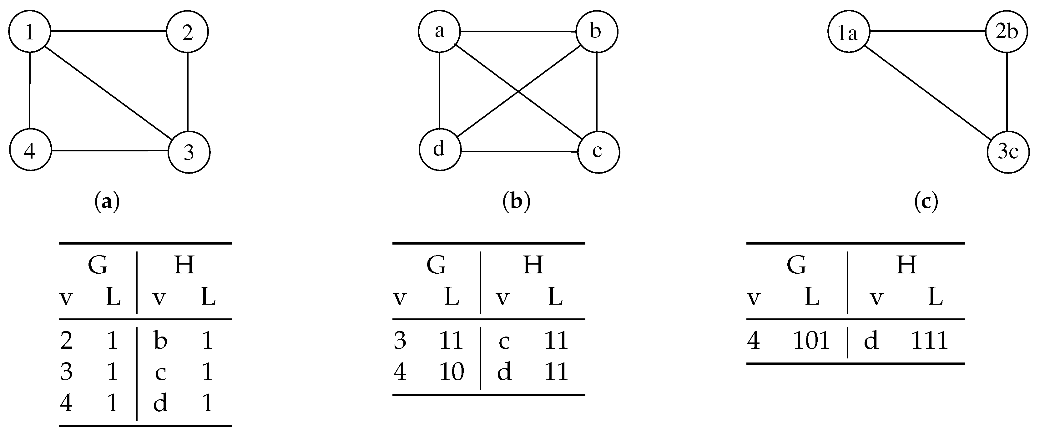
Let us suppose we have the two undirected graphs G and H represented in Figure 2a,b. As in Figure 1, we consider simple graphs for the sake of readability, and we report node labels, i.e., $\{1,2,3,4\}$ and $\{a,b,c,d\}$, only to identify all vertices uniquely. We compute the norms (or the cumulative cosine similarity) statically and just once at the beginning of the process (we discuss this issue further in Section 2.2), and that the suggested vertex sorting is $\{1,2,3,4\}$ for the first graph and $\{a,b,c,d\}$ for the second one. Initially, the mapping M between the vertices of G and H is an empty set. The algorithm adds a vertex pair to M at each recursion level. During the first recursion step, given our pre-computed vertex sorting, the procedure selects vertex 1 in G and maps this vertex to node a in H. The mapping M becomes equal to $M=\{1,a\}$. After that, the algorithm labels each unmatched vertex in G (H) according to whether it is adjacent to vertex 1 (a). For undirected graphs, adjacent vertices have the label 1, and non-adjacent vertices have the label 0. The table on the left-hand side of Figure 2 shows these labels. After that, the algorithm recurs, extending M with a new pair of vertices at each recursion level. If we follow the static order previously computed with the norms or the cumulative cosine similarity, M becomes $M=\{12,ab\}$ after a second recursion, and $M=\{123,abc\}$ after a third one. We report the remaining node labels in the center and the right-hand side tables. We cannot insert the last two vertices 4 and d in M because they have different labels; thus, the recursive procedure backtracks, searching for another (possibly longer) match in M.

Algorithm 1 illustrates the pseudo-code of the McSplit function revised using our approach. In lines 1–6, we update the current solution, and we check the termination condition using Equation (3) (evaluated at line 4. After the selection of a bidomain (line 8), we select a node from the “left” graph (line 9), which is, by convention, the first input graph. These lines are the first code section where the node heuristic takes effect. The original version of McSplit selects the node $v\in G$ with the highest degree inside the bidomain chosen in line 8. Then, vertex v is paired with each node $w\in H$, following the same scheme based on the node degree priority in line 11. For example, the first pair will be formed by the node v and w, both of maximum degree inside their respective graphs, in the selected bidomain. Our heuristic replaces the node degree heuristic in lines 9 and 11. As in the original algorithm, the most straightforward scheme is to compute the scores during an initialization step, before calling the $mcs$ function represented in the pseudo-code. After that, the priority scheme considers the maximum norm or the cumulative cosine similarity instead of the maximum degree.

Algorithm 1 mcs($G,H,M,incumbent,L$)

1: if  $\left|M\right|>\left|incumbent\right|$  then 2:     $incumbent\leftarrow M$ 3: end if 4: $bound\leftarrow \left|M\right|+calc\_bound\left(L\right)$ //Equation (3) 5: if  $bound\le \left|incumbent\right|$  then 6:     return $incumbent$ 7: end if 8: $bd\leftarrow select\_bidomain\left(L\right)$ // bidomain selection 9: $v\leftarrow select\_left\_node\left(bd\right)$ //node selection 10: remove v from bd 11: for each  $w\in bd$ do 12:     remove w from bd 13:     $M.push\left(\right(v,w\left)\right)$ //Add new pair to M 14:     $new\_L\leftarrow filter\_labels(L,v,w)$ //Generate new L set 15:     $incumbent\leftarrow mcs(G,H,M,incumbent,new\_L)$ 16:     M.pop() 17:     add w to $bd$ //w is added back 18: end for 19: if $bd.V_{l,g}$ is empty then 20:     remove $bd$ from L 21: end if  return  $mcs(G,H,M,incumbent,L)$

2.2. Computing Embedding Norms

Our embeddings are mathematical vectors with 64 dimensions, so we can manipulate them with many mathematical operators. In particular, we consider the operators that evaluate the similarity between two vectors. We base our first similarity check on the L2-norm. We compute the Euclidean norm from NeuroMatch embeddings assessed on the k-hop neighborhood of each node in both graphs. More specifically, we compute:

$$\begin{array}{ccc}L2\left(Z\right)& =& \sqrt{{\sum }_{i=1}^{D}Z{\left[i\right]}^2}\end{array}$$

(6)

where Z is a D-dimensional embedding vector. The L2-norm of such embeddings is higher for nodes of big and dense graphs, due to the NeuroMatch order constraint. Therefore, instead of simply considering a node’s degree, we believe in both the size and the order of the whole k-hop neighborhood.

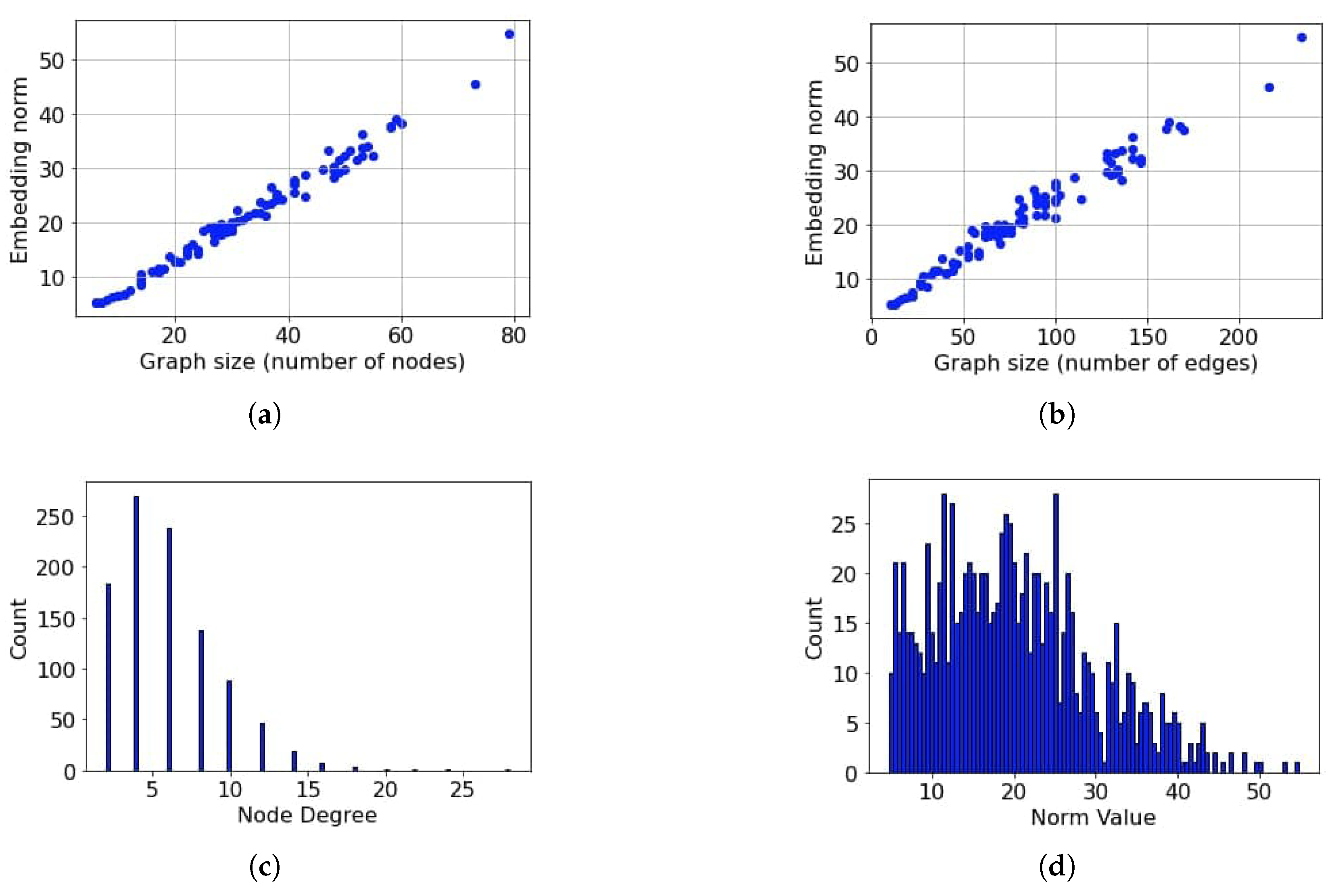
To confirm our conjecture, we run some experiments and report our analysis in Figure 3. We sample 100 subgraphs from a single graph with 100 nodes using a BFS with a depth limit of three. Then, we plot the norm value against the number of nodes (Figure 3a) and the number of edges (Figure 3b) for each graph.

Figure 3c,d show the distribution of the degree and norms, computed on a set of 10 graphs with 100 nodes each, respectively. Much less sparse than the norm value. Since the graph is connected and has 100 nodes, the node degree values could range from 1 to 100. On the contrary, most nodes have few neighbors, and the mean degree is about 5. Then, since McSplit breaks ties lexicographically, the performance of the node degree heuristic is much more dependent on random factors.

As described in Section 1.5.2, McSplit selects a new pair of nodes at each recursion call. Thus, the latest pair of vertices is added to the previously selected set of pairs at any new call along the search tree. Previously selected or non-selected pairs are not considered anymore when making a new selection and growing the current solution. This consideration influences how and when we compute (and possibly update) our embeddings. We initially consider the entire k-hop neighborhood around each node by only computing embeddings. However, as we go on with the algorithm, it could be wiser not to consider nodes already in the solution as part of any neighborhood. For example, it is possible to have the following situation. A vertex v has a large neighborhood, but this contains mainly vertices already included in the solution. In contrast, a vertex u has a small neighborhood, but this mostly incorporates nodes still available for future matching. In this condition, the norm evaluated at the beginning of the process can suggest a wrong vertex selection by prioritizing v over u.

To avoid this problem, the most obvious solution is to recompute embeddings (potentially) after each pair selection and, at the same time, ignore all vertices already selected in the current solution when sampling neighbors in the BFS procedure. This solution corresponds to removing all nodes in the current solution from the previously sampled subgraphs. Therefore, the nodes affected by this procedure will have smaller norms and a smaller priority moving along the selection process. At the same time, this process will increase the cost of computing embeddings. We will experimentally analyze this possibility in Section 3.7.

2.3. Computing the Cumulative Cosine Similarity

We aim to compute a score for each possible node pair as in the previous section. Given this target, the dot product is another metric assessing the similarity of two vectors with 64 dimensions. In particular, as two vectors are normalized, the dot product returns the cosine of the angle between the two vectors in two-dimensional space. Consequently, since we base the affinity of two nodes on their cosine, this metric is called cosine similarity, and it represents the similarity of their respective k-hop neighborhood. Thus, nodes with very similar neighborhoods have a higher similarity score. In this case, we sort the vertices of the graph based on the sum of the value of the cosine similarity computed between one node of G and all nodes of H. This cumulative metric is called cumulative cosine similarity (CCS). The main advantage of considering CCS is that the score of each node is obtained by reasoning on both graphs, whereas the heuristics based on the norm and the degree consider only a single graph.

Figure 4a,b show two pairs of graphs with a very different CCS, i.e., 1.0 in the first set and 0.22 in the second. The two figures show how CCS tends to be higher for similar (possibly isomorphic) graphs.

To compute the CCS, we proceed as follows. Given two graphs G and H, in the first step, we compute a matrix M where $M_{vw}$ is the cosine similarity score between node $v\in G$ and node $w\in H$. Then, we compute the score of each node in G as the sum of values on the corresponding row in M, while the scores of nodes in H are given by summing over columns. Specifically, for the nodes in G, we compute:

$$\begin{array}{ccc}CCS\left(v\right)& =& \sum _{w=1}^{\left|H\right|}{Z}_v·Z_w\end{array}$$

(7)

$Z_v$ and $Z_w$ are, the embedding vectors of node $v\in G$ and node $w\in H$, respectively. Notice that we do not normalize the result of the sum, as normalization would mean dividing every value by the same number. This score reflects how frequently a subgraph, sampled from one graph and represented by a node k-hop neighborhood, is found inside the other graph. These nodes are more likely to be matched or part of a big solution. Therefore, we give these nodes a higher priority.

2.4. Optimizations

Given an anchor node v, the value of k controls the depth of the breadth-first visit used to build our k-hop neighborhood subgraphs. In other words, we can see k as the eccentricity of the anchor node in the sampled subgraph. At the same time, we use a GNN with a pre-defined number of layers j to compute the embeddings. It is worth noticing that a GNN with j layers computes an embedding for the anchor node v by aggregating and transforming information gathered from its j-hop neighbors. Since we first sample a k-hop neighborhood subgraph using a BFS and then use j layers in the GNN, if $k>j$, all nodes at a distance $d>j$ from the anchor vertex would not be considered. Therefore, the number of layers j has to be consistently larger than or equal to the value of k to ensure that the information coming from all nodes will propagate to the anchor.

Theoretically, larger values of k (and j) should yield a more precise estimate and superior node ordering as the anchor node neighborhood is analyzed with greater depth. However, as demonstrated in the experimental section, our empirical findings reveal a diminishing return: Increasing k beyond a certain point offers no additional improvements in the number of graph pairs solved. Given that the computational cost of our heuristic increases proportionally with k, we empirically determined that $k=8$ serves as an optimal threshold, beyond which further graph analysis provides no significant benefits. Analysis of nodes too distant from the anchor node may introduce interdependencies among anchors, thereby potentially nullifying the unique contributions of individual node analyses.

As the computations performed with different values of k are independent, it is possible to speed up the process using parallel computing. In the current implementation, we use a trivial approach running in parallel 16 tasks (processes or threads), i.e., one for each value of k, 8 for the norm, and 8 for the CCS heuristic. From the memory point of view, running 16 tasks in parallel is generally not a problem, as each of them uses a limited quantity of memory. Moreover, when we adopt multi-threading, we can share part of the information (such as the graph representation) among the different threads. If we need to reduce the resource usage, we can also check the status of each task at a regular time interval (e.g., every 5–10% of the total available time) and stop the task that appears to be the slowest. To further speed up our computation, we can also exploit the parallelism capability of a Graphical Processing Unit (GPU). Since in a GPU, each thread warp is generated by multiples of 32 threads, having only one thread working means that 31 threads remain idle, nullifying the advantages of the GPU. Thus, we run 32 tasks in parallel for each graph pair, and divide the sampled subgraphs into batches of 32 units before loading them into the GPU memory. This process allows the GPU to spend less time in idle states, reducing the computation times.

3. Results

In this section, we first describe our experimental settings (Section 3.1) and our graph benchmarks (Section 3.2). Then, we show the efficiency of the norm heuristic (introduced in Section 2.2) and the CCS approach (described in Section 2.3) to transform depth-first into best-first searches and compare those results with McSplit and McSplitRL. We report our results in Section 3.3, Section 3.4, Section 3.5, and Section 3.6, respectively. Section 3.7 reports an analysis of our results when sorting is repeated at each recursion step (as described at the end of Section 2.2). Finally, Section 3.8 reports some summarizing results.

The complete code and all the details for reproducing the experiments are available under the GNU General Public License v3.0 (https://github.com/stefanoquer/Maximum-Common-Subgraph-Neuromatch, accessed on 1 July 2024).

3.1. Settings

We wrote our implementations in C++, the same language used to implement the original version of McSplit. However, instead of sorting the vertices using their degree, we load an arbitrary score vector, which we then use to decide in which order to pair graph nodes and, as a consequence, traverse the recursion tree. The score vectors are pre-computed using a Python script, version 3.10 (Python Software Foundation, https://www.python.org/). The script exploits the Pytorch framework, the Pytorch Geometric, and the DeepSnap libraries used in NeuroMatch. This approach leverages the efficiency of the neural network environment embedded in the Python framework with the performance of the C/C++ code to implement recursive branch-and-bound functions. Efficiency is essential because the Python implementation of the original algorithm, which is the most time-consuming part of the process, is from one to two orders of magnitude slower than the original one. On the contrary, computing the node embeddings with the Python script requires about one second, on average. This time is usually negligible in our experiments, and we can undoubtedly reduce it by using a C/C++ process or by including the computation inside the compiled program itself. However, in all cases, we consider the time to compute node embeddings included in our timeout.

In our work, we employed the publicly available, pre-trained NeuroMatch model, as described by Ying et al. [31]. We selected the NeuroMatch model as it shares critical conceptual similarities with the MCS. NeuroMatch is primarily trained to learn subgraph embeddings that satisfy strong subgraph relationship constraints (transitivity, anti-symmetry, intersection, etc.), making it capable of encoding k-hop structural information for nodes in an order-preserving manner. The original NeuroMatch pre-training used a diverse combination of synthetic and real-world graph datasets and focused on the general task of subgraph matching and inclusion, not exclusively on MCS instances. This feature means that while NeuroMatch is not trained directly on MCS-labeled datasets, it is optimized to produce node and subgraph embeddings that reflect accurate subgraph relationships (an essential prerequisite for the heuristics we propose). The core requirement for our approach is that the embeddings reflect structural similarity and neighborhood inclusion, not necessarily MCS labels per se. Its loss function is specifically designed to distinguish when one graph is a subgraph of another, which is highly relevant to the MCS task, where the discovery of large common subgraphs is the objective.

Our experiments found that the pre-trained model performed robustly on the standard MCS benchmarks (unlabeled, undirected graphs). We did not perform further fine-tuning, as our approach does not require supervision specific to MCS instances, and, as suggested by the authors, we only selected the required hyperparameters. We use the embeddings as feature vectors to rank and choose node matches. NeuroMatch does not rely on a specific GNN, and it can exploit different state-of-the-art models, such as the Graph Convolutional Network, GraphSAGE, and Graph Isomorphism Network. Following the original paper [31], we use an 8-layer GraphSAGE and an embedding space with 64 dimensions. This configuration is supposed to maximize the accuracy, i.e., the number of correct matchings performed by NeuroMatch. We also run experiments with the parameter k ranging from 1 to 8. As we fixed the number of GNN layers to 8, larger values of k would not change the results, as nodes at a distance higher than eight would be ignored.

Moreover, we view the off-the-shelf model as a positive aspect, since more domain-specific training or fine-tuning (for example, using MCS solution data) could further improve results. NeuroMatch’s architecture is model-agnostic and compatible with applying other graph neural network backbones and training regimes, allowing its adaptation to new graph domains or MCS variants. Thus, while the NeuroMatch pre-training is not MCS-specific, its subgraph-centric training regime, order-preserving embeddings, and demonstrated transferability to subgraph discovery tasks support its applicability to MCS heuristics as presented. However, we acknowledge the potential for domain-specific fine-tuning, especially for labeled, directed, or structurally distinct graphs. We plan to explore this further, as mentioned in our discussion on future work.

We run our experiments on an Intel i9 10900KF CPU running at 3.7 GHz, with 10 cores and 20 threads, and an NVIDIA RTX 3070 GPU for the embedding computation. We use Ubuntu 24.04.1 LTS as the operating system.

We compare our results against the original version of McSplit [23] and McSplitRL [25], which have been used as a starting point for several other heuristics, such as McSplitLL [26] and McSplitDAL [27] (We do not compare against GLSearch [29] as it targets the connected variant of MCS without options to use it to generate disconnected MCS. Moreover, although we contacted the authors [33], we could not train the model from scratch, and running the public implementation against different datasets was impossible as it delivered inefficient or wrong results in most experiments. We also try other variants of the original procedure, always based on Reinforcement Learning, but all suffer limitations which lead them to find solutions of small final size). The portfolio method presented by Quer et al. [30] targets the reduction in the computation times. Still, it essentially visits the same space as the original method, and a comparison could not provide additional information.

3.2. Benchmarks

To run their experiments, Liu et al. [25] select 24,761 instances of “average difficulty”, and remove from this set all graph pairs that either ran out of time or could not be solved within a timeout of 10 s. They prove that on the remaining 2790 instances, McSplitRL can solve 140 more instances than McSplit.

We use graph instances retrieved from the original GitHub repository of McSplit (https://github.com/jamestrimble/ijcai2017-partitioning-common-subgraph/tree/master/mcs-instances, accessed on 1 July 2024). Among those benchmarks, we select 500 random graph pairs extracted uniformly from the different families (i.e., completely random, 2D, 3D, etc.). For our comparison, we increase the timeout to 3000 s (i.e., 50 min). We divide the 500 graph pairs into two categories to compare results appropriately. The first includes the graph pairs that the original McSplit implementation can solve in the slotted time (119 instances). The second one consists of the cases that run out of time in 50 min (the remaining 381 pairs). In the first set, we compare the computation time. In the second set, we first compare the size of the common subgraph found by the different heuristics; then, when the graphs have the same size, we compare the number of recursions required to compute such a result. Notice that the number of recursions is strictly related to the computation time, but much less to the code efficiency and the hardware platform used to run the experiments. Moreover, the number of recursions gives a specific indication of the convergence speed of the process.

3.3. The Norm Heuristic Against McSplit

Table 1. The table details the number of graph pairs (out of 500) in which one specific tool is superior, that is, it calculates the largest result, or an equivalent result in fewer recursion steps. The original McSplit is confronted with our tool using the embedding norm heuristic, with different sizes k of the embedding. The table also reports the specific performances obtained with each value of k.

		Norm
Completion	McSplit	Total	k = 1	k = 2	k = 3	k = 4	k = 5	k = 6	k = 7	k = 8
Within timeout	50	59	22	13	11	6	4	1	1	0
	10%	12%	4%	3%	2%	1%	1%	0%	0%	0%
Timeout expired	101	290	105	45	60	18	12	21	19	10
	20%	58%	21%	9%	12%	4%	2%	4%	4%	2%

compares the performance of our norm heuristic with the original McSplit. The 500 graph pairs are divided into two categories as described in Section 3.2. Thus, we compare the computation time in the first column to find the maximal solution. In the second one, we compare the size of the common subgraph found by the different heuristics or the number of recursions required to compute such a result. For each row, we report absolute and percentage results.

The table shows that McSplit is faster on 54 cases and the norm heuristic on 64 other cases if we consider the instances that can be solved in the slotted time. The first row indicates cases where McSplit can find the MCS and solve the problem, whereas the second row reports the instances where it runs out of time. Overall, our norm heuristic beats McSplit by about 70% (12% + 58%) of the cases, providing either a more extensive or equivalent solution in less time. For the norm heuristic, we report the number of winning instances for each value of k from 1 to 8. Thus, our data shows that, among the 59 cases in which it wins, the norm heuristic is faster than McSplit in 22 instances with $k=1$, 13 cases with $k=2$, etc. Notice that the computations performed with different values of k are independent. Consequently, as introduced in Section 2.4, it is possible to solve the problem using parallel computing and running independent tasks for each value of k. From the memory point of view, this is not a problem as each task uses a limited quantity of memory.

3.4. The Norm Heuristic Against McSplitRL

Table 2. The table details the number of graph pairs (out of 500) in which one specific tool is superior, that is, it calculates the largest result, or an equivalent result in fewer recursion steps. The original McSplitRL is confronted with our tool using the embedding norm heuristic, with different sizes k of the embedding. The table also reports the specific performances obtained with each value of k.

		Norm
Completion	McSplitRL	Total	k = 1	k = 2	k = 3	k = 4	k = 5	k = 6	k = 7	k = 8
Within timeout	55	57	20	11	11	8	5	2	0	0
	11%	11%	4%	2%	2%	2%	1%	1%	0%	0%
Timeout expired	100	288	113	47	40	27	12	20	20	9
	20%	58%	23%	9%	8%	5%	2%	4%	4%	2%

shows the performance of the norm heuristic compared with McSplitRL. We organize it as Table 1. In particular, McSplitRL provides the best results on the most minor graph pairs and the worst on the largest ones. Overall, we can beat McSplitRL in about 69% of the graph pairs.

3.5. The CCS Heuristic Against McSplit

Table 3. The table details the number of graph pairs (out of 500) in which one specific tool is superior, that is, it calculates the largest result, or an equivalent result in fewer recursion steps. The original McSplit is confronted with our tool using the CCS heuristic, with different sizes k of the embedding. The table also reports the specific performances obtained with each value of k.

		Cumulative Cosine Similarity
Completion	McSplit	Total	k = 1	k = 2	k = 3	k = 4	k = 5	k = 6	k = 7	k = 8
Within timeout	20	85	35	17	12	10	6	3	2	0
	4%	17%	7%	3%	2%	2%	1%	0%	0%	0%
Timeout expired	32	363	68	65	60	51	42	36	29	12
	6%	73%	14%	13%	12%	10%	8%	7%	6%	2%

compares our CCS heuristic with the original version of McSplit. In particular, the first two columns show which method brings improvements more frequently, and the other ones report results for single values of k. The first row of the table analyzes the instances that McSplit can solve in the slotted time. On these 105 graph pairs, our CCS heuristic wins in 80.9% of the cases (85/105). Many of the considerations reported for the norm heuristic are also valid for the CCS strategy. Nevertheless, CCS is more efficient, and on all graph pairs, it improves the original strategy in 90% of the cases.

To better understand why the CCS heuristic has an edge over the norm one, we can try to consider the two measures better. For example, Haokai et al. [34] fuse multi-source heterogeneous data to predict online car-hailing order cancellation probability. Their ablation study shows that combining all external factors leads to the best prediction accuracy. This feature suggests that a more comprehensive, global understanding of the factors (contrasting local features) is crucial for better prediction. Once noticed, our L2 norm of embedding primarily reflects the size and density of a node’s local k-hop neighborhood within its graph. While this is valuable, it does not inherently consider how well that local structure “fits” into another graph. In other words, the L2 norm computes a node’s embedding considering information from each graph context. Conversely, as applied in our context, CCS calculates a score for each node based on the sum of cosine similarities between that node’s embedding in one graph and all nodes’ embeddings in the other. This feature means CCS is inherently considering information from both graphs simultaneously when determining a node’s priority. This characteristic is analogous to multi-source data fusion because it integrates information from two distinct sources (the two graphs) to make a more informed decision about node pairing. Our results are a direct experimental demonstration of how “more comprehensive” and “contextual” features lead to better predictions. The CCS metric, by considering the compatibility of a node with all nodes in the other graph, essentially leverages a “richer set of features” leading to a better prediction.

3.6. The CCS Heuristic Against McSplitRL

Table 4. The table details the number of graph pairs (out of 500) in which one specific tool is superior, that is, it calculates the largest result, or an equivalent result in fewer recursion steps. The original McSplitRL is confronted with our tool using the CCS heuristic, with different sizes k of the embedding. The table also reports the specific performances obtained with each value of k.

		Cumulative Cosine Similarity
Completion	McSplitRL	Total	k = 1	k = 2	k = 3	k = 4	k = 5	k = 6	k = 7	k = 8
Within timeout	18	87	27	18	13	10	10	7	2	0
	4%	17%	5%	4%	3%	2%	2%	1%	0%	0%
Timeout expired	25	370	73	69	64	50	44	42	15	13
	5%	74%	15%	14%	13%	10%	9%	8%	3%	3%

compares our CCS heuristic with McSplitRL. The format of the table is similar to the previous ones. When the original approach can end the search within the timeout, CCS beats McPlitRL in 82% of the instances (87 wins in 105 cases). When the timeout expires, CCS beats McSplitRL in 93%.

Table 5. The table compares the CCS heuristic with the original McSplit implementation and the McSplitRL strategy at the same time.

Completion	McSplit	McSplitRL	CCS ($\mathit{k}=1–8$)
Within timeout	13	9	85
	3%	2%	17%
Timeout expired	22	10	361
	4%	2%	72%

compares our CCS heuristic to McSplit and McSplitRL simultaneously, showing how many instances each heuristic can solve better or faster than the other methods. Overall, our CCS strategy beats the previous methods (producing a larger incumbent or equivalent one in less time or with fewer recursions) in 89% of the cases (17% + 72%).

Figure 5 shows an in-depth analysis of our CCS heuristic and McSplit behavior on two graph pairs. The y-axis reports the solution size, whereas the x-axis indicates the number of recursions on a logarithmic scale for readability. Each dot of the two graphics represents the first time the heuristic reaches a specific solution size. This size is updated frequently for the first 748 recursions; after that, value updates become sparse and, as in all previous experiments, both heuristics run with a timeout of 50 min. Figure 5a shows a case in which the CCS heuristic finds larger incumbents before McSplit in all cases, and it also returns a large solution. This behavior is prevalent in our experiments, with few exceptions among the instances that we cannot improve. Figure 5b analyzes one of those cases, i.e., a graph pair in which McSplit finds a solution more extensive than the one found by the CCS heuristic when the time expires. However, even in this case, most of the time, our heuristic holds a better incumbent than McSplit, and with any shorter timeout, it would have improved the result returned by McSplit. As a result, the CCS heuristic often improves the original algorithms by finding more extensive solutions in a shorter amount of time.

3.7. Balancing Computational Cost and Solution Quality: Dynamic Heuristic Updates

As introduced in Section 2.2, a norm evaluated at the beginning of the process can suggest a wrong vertex selection. However, dynamically recomputing embeddings could enhance solution quality by providing more relevant heuristic information during the search. Unfortunately, this approach incurs a significant computational cost. This section addresses this trade-off by analyzing the impact of recomputing embedding norms at each recursion step.

Table 6. Comparing the original McSplit with our tool when we recompute the norm heuristic at each recursion step.

Heuristic	Our Tool Wins	McSplit Wins
Single Norm Computation	59	50
Multiple Norm Computation	72	44

reports a comparison between McSplit and our norm heuristic in which we recompute the norms at each recursion step. The value of k is set to one. When the norm recomputation is performed at each recursion, it leads to a higher number of wins (72 cases) compared to the original case (59 cases) presented in Table 1. This table suggests an improvement in solution quality for some test instances. However, this improvement comes at a substantial computational expense: Computing embeddings at the beginning of the process is efficient, accounting for only 0.1–0.4% of the total allocated time. In stark contrast, recomputing norms at each recursion step can consume over 95% of the allotted time, drastically limiting the number of recursions the algorithm can perform.

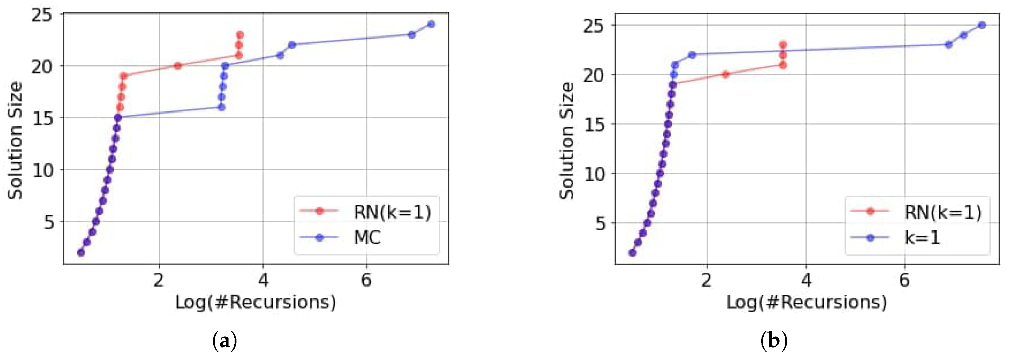
This behavior significantly reduces the overall computational efficiency, as illustrated in Figure 6. The plot represents the behavior on a unique graph pair, but the behavior is typical for many benchmarks in our dataset. Our heuristic with norm recomputation (RN) outperforms the McSplit original heuristic (MC) up to a certain number of recursions (left-hand side plot). After that number, norms lose power, and the original heuristic converges faster. A similar behavior is obtained when we compare our heuristic with and without the norm recomputation (right-hand side graphic).

This characteristic presents a clear challenge, i.e., balancing the computational cost of dynamic heuristic updates with the potential for improved solution quality. The current strategy of recomputing embeddings at every step is impractical due to its high computational overhead. Logic suggests that a more nuanced approach is required. One possible strategy is to recompute the norm if the algorithm does not improve the solution size after a pre-defined time or a pre-defined number of recursions. We can implement this methodology in different ways. The naive approach stops the algorithm at any branching point, recomputes the norm, and restarts the algorithm with the new norms. A better approach backtracks to a promising branching point and then computes the norms. For example, in [29], the algorithm backtracks to the branching point with the largest action space, i.e., the one with the most possible branches. This procedure can also help to avoid falling into a local optimum.

3.8. Summaryzing Results

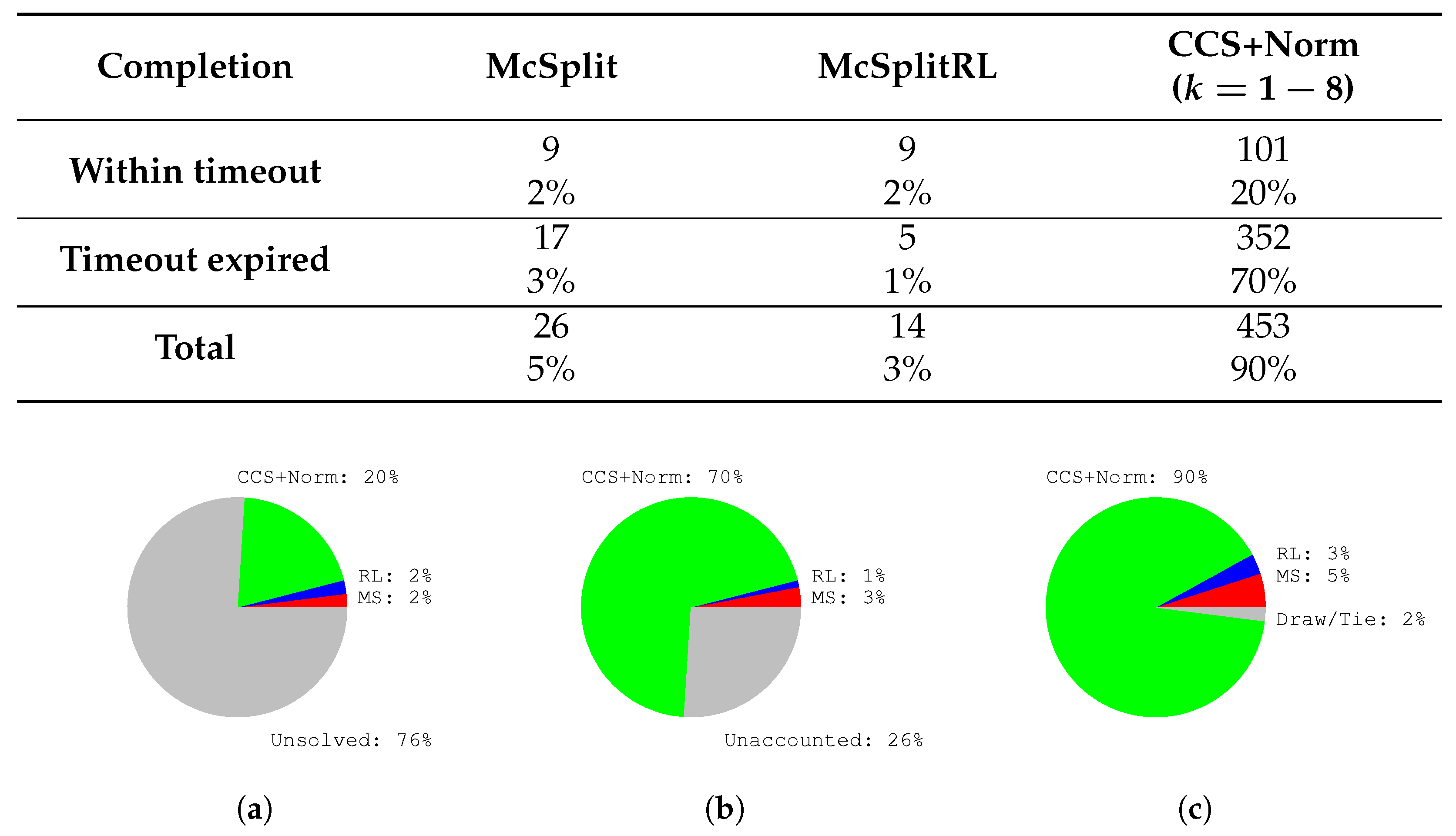
This section serves as a comprehensive summary of the experimental results for our MCS approach against the state-of-the-art McSplit and McSplitRL algorithms. Figure 7 includes a table and three pie plots. The table consolidates findings from earlier analyses, demonstrating the cumulative strength of combining the L2 norm with the CCS heuristic. This combination can win in 20% of the cases in which McSplit can thoroughly analyze the problem, and in 70% of the instances in which a partial (potentialy non optimum) solution is found. The dominance in all cases (over 90% of best results) highlights its reliability and generalizability. It is apparent that the trade-off between computational cost and search effectiveness, previously highlighted, is resolved in favor of the combined method, which requires only minor extra computation for substantial gains.

The three pie plots graphically reinforce the statistical findings from the table. They depict the overwhelming proportion of successful instances attributed to the CCS+Norm strategy. Each plot covers a subset: solved within timeout, unsolved within timeout, and the aggregate. The visual emphasis is on the absolute performance lead and the shrinking fraction of challenging “Unsolved”, “Unaccounted”, or “Draw/Tie” cases.

To sum up, this analysis demonstrates that integrating neural-embedding heuristics into a branch-and-bound MCS solver creates a new state of the art for both efficacy and efficiency.

4. Conclusions and Future Works

This work introduces a branch-and-bound strategy significantly enhanced by Graph Neural Network (GNN) heuristics. Our approach leverages NeuroMatch to compute embeddings for each k-hop neighborhood centered on every anchor vertex within a graph. These embeddings, learned by a Graph Neural Network, are then utilized to prioritize nodes during branching, employing their L2-norm and cosine similarity instead of traditional node degrees. This information guides the sorting of vertices for pairing, facilitating the discovery of Maximum Common Subgraphs (MCS).

Our experiments explored various values for the k-parameter. While the norm heuristic did not consistently outperform the original heuristic in every instance, it demonstrated superior performance in approximately half of our test cases. A clear advantage was observed when considering different orderings derived from varying k values. The cumulative cosine similarity (CCS) heuristic notably showed more consistent improvements across different k values. By combining the best k values from both the norm and CCS heuristics, we surpassed the node-degree heuristic in most MCS problem instances.

Among the limitations of our current strategy, the most significant is the computational expense associated with dynamically updating node embeddings at each recursion step. While theoretically beneficial for providing more relevant heuristic information during the search, frequent recomputation dramatically increases the overall time budget. For instance, computing embeddings initially accounts for a mere 0.1–0.4% of the total budget time. However, recomputing norms at each recursion can consume over 95% of the allotted time, severely limiting the number of recursions the algorithm can perform. This trade-off between the quality of heuristic information and computational cost is a critical challenge.

Currently, sorting vertices based on node embeddings cannot be effectively iterated at every recursion step, as this process does not consistently improve the initial vertex order. Furthermore, our current embedding representation has limitations: We directly optimize embeddings rather than a set of parameters, which can lead to different node embeddings being generated from the same parameter set. Additionally, our embeddings do not support node features and are transductive, meaning they can only be generated for nodes encountered during training.

Addressing these limitations is a primary focus for our future work. We propose to investigate adaptive strategies for embedding recomputation, similar to approaches seen in other domains like Deep Reinforcement Learning for spatio-temporal models, where gradient accumulation is used to adapt behavior. An adaptive strategy would recompute embeddings only when the algorithm fails to improve the solution size after a predefined time or number of recursions. This feature would prevent unnecessary computations while ensuring the heuristic remains fresh and relevant, especially when the search might be stuck in a local optimum or when the current heuristic becomes stale. This adaptive approach would balance computational cost with performance gains by strategically updating the heuristic information.

In this area, a smarter use of parallel architecture, ranging from multi-core (CPU) to many-core (GPU), can provide data parallel slicing, thus providing quantitative evidence (memory usage, convergence speed, and accuracy metrics) to demonstrate its power and scalability.

Furthermore, we aim to extend our approach to work with a broader variety of graph pairs and to find an alternative to the McSplit bidomain heuristic, which currently limits our branching choices. NeuroMatch’s adaptability to labeled, directed, and larger graphs suggests promising avenues for expansion. We also plan to verify the behavior of supervised methods for similar tasks and conduct extensive experiments on large graphs to evaluate the scalability of this new approach thoroughly.

References

1. Gross, J.L.; Yellen, J.; Anderson, M. Graph Theory and Its Applications, 3rd ed.; Chapman & Hall/CRC: Boca Raton, FL, USA, 2018. [Google Scholar]
2. Dalke, A.; Hastings, J. FMCS: A Novel Algorithm for the Multiple MCS Problem. J. Cheminform. 2013, 5, O6. [Google Scholar] [CrossRef]
3. Milgram, S. The Small World Problem. Psychol. Today 1967, 2, 60–67. [Google Scholar]
4. Brin, S.; Page, L. The Anatomy of a Large-Scale Hypertextual Web Search Engine. Comput. Netw. ISDN Syst. 1998, 30, 107–117. [Google Scholar] [CrossRef]
5. Park, Y.; Reeves, D.S.; Stamp, M. Deriving Common Malware Behavior through Graph Clustering. Comput. Secur. 2013, 39, 419–430. [Google Scholar] [CrossRef]
6. Zimmermann, T.; Nagappan, N. Predicting Subsystem Failures using Dependency Graph Complexities. In Proceedings of the 18th IEEE International Symposium on Software Reliability (ISSRE ’07), Trollhattan, Sweden, 5–9 November 2007; pp. 227–236. [Google Scholar] [CrossRef]
7. Angione, F.; Bernardi, P.; Calabrese, A.; Cardone, L.; Niccoletti, A.; Piumatti, D.; Quer, S.; Appello, D.; Tancorre, V.; Ugioli, R. An Innovative Strategy to Quickly Grade Functional Test Programs. In Proceedings of the IEEE International Test Conference (ITC), Anaheim, CA, USA, 23–30 September 2022; pp. 355–364. [Google Scholar] [CrossRef]
8. Bron, C.; Kerbosch, J. Algorithm 457: Finding all Cliques of an Undirected Graph. Commun. ACM 1973, 16, 575–577. [Google Scholar] [CrossRef]
9. Barrow, H.G.; Burstall, R.M. Subgraph Isomorphism, Matching Relational Structures and Maximal Cliques. Inf. Process. Lett. 1976, 4, 83–84. [Google Scholar] [CrossRef]
10. Levi, G. A Note on the Derivation of Maximal Common Subgraphs of Two Directed or Undirected Graphs. Calcolo 1973, 9, 341–352. [Google Scholar] [CrossRef]
11. Bahiense, L.; Manić, G.; Piva, B.; de Souza, C.C. The Maximum Common Edge Subgraph Problem: A Polyhedral Investigation. Discret. Appl. Math. 2012, 160, 2523–2541. [Google Scholar] [CrossRef]
12. Vismara, P.; Valery, B. Finding Maximum Common Connected Subgraphs Using Clique Detection or Constraint Satisfaction Algorithms. In Proceedings of the Modelling, Computation and Optimization in Information Systems and Management Sciences, Metz, France, 8–10 September 2008; Le Thi, H.A., Bouvry, P., Pham Dinh, T., Eds.; Springer: Berlin/Heidelberg, Germany, 2008; pp. 358–368. [Google Scholar]
13. McCreesh, C.; Ndiaye, S.N.; Prosser, P.; Solnon, C. Clique and Constraint Models for Maximum Common (Connected) Subgraph Problems. In Proceedings of the Principles and Practice of Constraint Programming, Toulouse, France, 5–9 September 2016; Rueher, M., Ed.; Springer Nature: Cham, Switzerland, 2016; pp. 350–368. [Google Scholar] [CrossRef]
14. Yu, X.; Liu, Z.; Fang, Y.; Zhang, X. Learning to Count Isomorphisms with Graph Neural Networks. In Proceedings of the Thirty-Seventh AAAI Conference on Artificial Intelligence and Thirty-Fifth Conference on Innovative Applications of Artificial Intelligence and Thirteenth Symposium on Educational Advances in Artificial Intelligence, AAAI’23/IAAI’23/EAAI’23, Washington, DC, USA, 7–14 February 2023; AAAI Press: Washington, DC, USA, 2023. [Google Scholar] [CrossRef]
15. Wang, Z.; Zhang, Z.; Ma, T.; Chawla, N.V.; Zhang, C.; Ye, Y. Beyond Message Passing: Neural Graph Pattern Machine. arXiv 2025. [Google Scholar] [CrossRef]
16. Hashemi, M.; Gong, S.; Ni, J.; Fan, W.; Prakash, B.A.; Jin, W. A Comprehensive Survey on Graph Reduction: Sparsification, Coarsening, and Condensation. In Proceedings of the Thirty-Third International Joint Conference on Artificial Intelligence, IJCAI ’24, Jeju, Republic of Korea, 3–9 August 2024. [Google Scholar] [CrossRef]
17. Liu, Y.; Bo, D.; Shi, C. Graph Condensation via Eigenbasis Matching. In Proceedings of the 41st International Conference on Machine Learning, Vienna, Austria, 21–27 July 2024. [Google Scholar]
18. Guidobene, D.; Cera, G. Improved Dynamics for the Maximum Common Subgraph Problem. arXiv 2024. [Google Scholar] [CrossRef]
19. Yu, K.; Wang, K.; Long, C.; Lakshmanan, L.; Cheng, R. Fast Maximum Common Subgraph Search: A Redundancy-Reduced Backtracking Approach. Proc. ACM Manag. Data 2025, 3, 1–27. [Google Scholar] [CrossRef]
20. Roy, I.; Chakrabarti, S.; De, A. Maximum Common Subgraph Guided Graph Retrieval: Late and Early Interaction Networks. In Proceedings of the 36th International Conference on Neural Information Processing Systems, NIPS ’22, Red Hook, NY, USA, 28 November–9 December 2022. [Google Scholar]
21. Lu, K.; Zhang, Y.; Xu, K.; Gao, Y.; Wilson, R.C. Approximate Maximum Common Sub-graph Isomorphism Based on Discrete-Time Quantum Walk. In Proceedings of the 2014 22nd International Conference on Pattern Recognition, Stockholm, Sweden, 24–28 August 2014; pp. 1413–1418. [Google Scholar] [CrossRef]
22. Dilkas, P. Algorithm Selection for Maximum Common Subgraph. Bachelor’s Thesis, University of Glasgow, Glasgow, Schotland, 2018. [Google Scholar]
23. McCreesh, C.; Prosser, P.; Trimble, J. A Partitioning Algorithm for Maximum Common Subgraph Problems. In Proceedings of the 26th International Joint Conference on Artificial Intelligence, IJCAI-17, Melbourne, Australia, 19–25 August 2017; AAAI Press: Washington, DC, USA, 2017; pp. 712–719. [Google Scholar]
24. Trimble, J. Partitioning Algorithms for Induced Subgraph Problems. Ph.D. Thesis, University of Glasgow, Glasgow, UK, 2023. [Google Scholar]
25. Liu, Y.; Li, C.M.; Jiang, H.; He, K. A Learning Based Branch and Bound for Maximum Common Subgraph Related Problems. In Proceedings of the AAAI Conference on Artificial Intelligence, New York, NY, USA, 7–12 February 2020; Volume 34, pp. 2392–2399. [Google Scholar] [CrossRef]
26. Zhou, J.; He, K.; Zheng, J.; Li, C.M.; Liu, Y. A Strengthened Branch and Bound Algorithm for the Maximum Common (Connected) Subgraph Problem. In Proceedings of the Thirty-First International Joint Conference on Artificial Intelligence, Vienna, Austria, 23–29 July 2022. [Google Scholar] [CrossRef]
27. Liu, Y.; Zhao, J.; Li, C.M.; Jiang, H.; He, K. Hybrid Learning with New Value Function for the Maximum Common Induced Subgraph Problem. In Proceedings of the Thirty-Seventh AAAI Conference on Artificial Intelligence, Washington, DC, USA, 7–14 February 2023. [Google Scholar] [CrossRef]
28. Bai, Y.; Xu, D.; Gu, K.; Wu, X.; Marinovic, A.; Ro, C.; Sun, Y.; Wang, W. Neural Maximum Common Subgraph Detection with Guided Subgraph Extraction. OpenReview 2020. preprint. [Google Scholar]
29. Bai, Y.; Xu, D.; Sun, Y.; Wang, W. GLSearch: Maximum Common Subgraph Detection via Learning to Search. In Proceedings of the 38th International Conference on Machine Learning, Virtual, 18–24 July 2021; Meila, M., Zhang, T., Eds.; Proceedings of Machine Learning Research. PMLR: New York, NY, USA, 2021; Volume 139, pp. 588–598. [Google Scholar]
30. Quer, S.; Marcelli, A.; Squillero, G. The Maximum Common Subgraph Problem: A Parallel and Multi-Engine Approach. Computation 2020, 8, 48. [Google Scholar] [CrossRef]
31. Ying, R.; Lou, Z.; You, J.; Wen, C.; Canedo, A.; Leskovec, J. Neural Subgraph Matching. arXiv 2020. [Google Scholar] [CrossRef]
32. Grover, A.; Leskovec, J. node2vec: Scalable Feature Learning for Networks. In Proceedings of the 22nd ACM SIGKDD International Conference on Knowledge Discovery and Data Mining, KDD ’16, New York, NY, USA, 13–17 August 2016; pp. 855–864. [Google Scholar] [CrossRef]
33. Bai, Y.; Xu, D.; Sun, Y.; Wang, W. (Department of Computer Science, University of California, Los Angeles, CA, USA). Personal communication, 2023.
34. Sun, H.; Lv, Z.; Li, J.; Xu, Z.; Sheng, Z.; Ma, Z. Prediction of Cancellation Probability of Online Car-Hailing Orders Based on Multi-source Heterogeneous Data Fusion. In Proceedings of the Wireless Algorithms, Systems, and Applications: 17th International Conference, WASA 2022, Dalian, China, 24–26 November 2022; Proceedings, Part II. Springer: Berlin/Heidelberg, Germany, 2022; pp. 168–180. [Google Scholar] [CrossRef]
Figure 1. Given the graphs G (a) and H (b), Figures (c,d) report two different admissible MCSs (MCS(G, H)). Labels are shown only to identify the vertices uniquely.
Applsci 15 08920 g001
Figure 2. The two initial undirected and unlabeled graphs G (a) and H (b), and one possible common subgraph computed by McSplit MCS(G, H) (c), are reported on top. The labels (L) on the non-mapped vertices ( v V ) are reported in the following tables, with the mapping M changing from the empty set, to M = { 1 , a } , M = { 12 , a b } . and finally M = { 123 , a b c } .
Applsci 15 08920 g002
Figure 3. We evaluate our norm against the graph size as the number of vertices (a) and the number of edges (b). The norm tends to be higher with larger graphs. Figure (c) shows the distribution of the degree of the graph’s vertices. Figure (d) plots the distribution of the embeddings’ norm values with subgraphs sampled using a BFS.
Applsci 15 08920 g003
Figure 4. Figure (a) shows two graphs with a cosine similarity of 1. Figure (b) shows two graphs with a cosine similarity of 0.22.
Applsci 15 08920 g004
Figure 5. A recursion-by-recursion comparison: Our CCS heuristic (with k = 3) against McSplit. The plot on the left-hand side (a) shows a case in which the CCS heuristic finds larger incumbents before McSplit and it also returns a large solution. The figure on the right-hand side (b) analyzes a peculiar case in which McSplit finds a solution more extensive than the one found by the CCS heuristic when the time expires.
Applsci 15 08920 g005
Figure 6. Comparison between McSplit (MC) and our tool using the L2 norm to sort vertices (RN). On the left-hand side (a), we consider our tool with L2 norm recomputation. On the right-hand side (b), we evaluate it without L2 norm recomputation.
Applsci 15 08920 g006
Figure 7. Comparison of McSplit and McSplitRL with our approach combining the L2 norm and the CCS heuristic. This combination wins in 20% of the cases in which McSplit terminates the computation of the MCS (a), in 70% of the instances in which a partial (potentially non optimum) solution is found (b), and in over 90% of all cases (considering both the previos categories, (c)). The three pie plots illustrate the same findings (from left to right) graphically.
Applsci 15 08920 g007