Physics Statistical Descriptor-Informed Deep Image Structure and Texture Similarity Metric as a Generative Adversarial Network Optimization Criterion for Three-Dimensional Gray-Scale Core Reconstruction

Abstract

Digital core refers to the use of three-dimensional physical imaging equipment and mathematical modeling to image the internal microstructure of a core and the use of computers to study the connectivity and pore distribution of the core microstructure. The digital core has emerged as a prominent research avenue in image processing in recent years. A three-dimensional (3D) image can be used to effectively study the microstructure and physical properties of a core. Three-dimensional reconstruction from two-dimensional core images is a crucial advancement in this field. Deep learning is advantageous in image reconstruction. However, when the traditional generative adversarial network (GAN) reconstruction method is adapted for reconstructing gray-scale core images, maintaining texture characteristics is difficult; additionally, it may produce blur artifacts in the GAN-generated gray-scale images. In this study, the physics statistical descriptor-informed deep image structure and texture similarity (PSDI-DISTS) metric, a higher-level metric than the traditional correlation function, is used as the loss function of the network, and a texture feature-constrained GAN (TFCGAN) model is proposed for reconstructing gray-scale core images. In addition, a balanced training strategy integrating L₁ and PSDI-DISTS losses is designed to optimize the model performance. The experimental results and seepage simulation analysis showed that TFCGAN can maintain the textural characteristics in the gray-scale core image reconstruction results. Furthermore, the reconstruction results exhibited seepage characteristics similar to those of the target.

1. Introduction

Cores are rock samples extracted from formations through drilling and can be used to study reservoir diagenesis and the state of oil and gas storage. Oil and gas are primarily stored in the pores of the core, and the microstructure of these pores directly determines their reserves and migration capacity. Therefore, studying the influence of the pore microstructure on the core’s macroscopic physical properties (such as permeability, electrical properties, and mechanical properties) is crucial for oil and gas exploration and development. Traditional physical property experiments focus primarily on the macroscale and are unable to investigate the physical properties of cores at the microscale of pores.

Digital cores, a field that has been proposed in recent years and stands at the intersection of digital image processing and petroleum geology, have become a current research hotspot. Using imaging equipment to image the microstructure within the core, computers can be used to study its connectivity and pore distribution, as well as to perform various simulations such as those for seepage, electrical properties, and mechanical properties. These calculations and simulations can provide fundamental research data and support subsequent petroleum exploration and development.

Current research in three-dimensional (3D) reconstruction of digital cores focuses on binary core images [1,2,3,4,5,6,7], wherein the minerals in rock samples are considered a single entity. The gray values of pixels in a 3D core CT image comprehensively reflect the differences in the X-ray absorption coefficients of different rock components. Real rock samples are composed of different components that exhibit different gray values under imaging equipment. Specifically, core parameter characteristics, such as permeability, electrical conductivity, and elastic modulus, also vary with the distribution of these components. Reconstructing gray-scale core images from a single two-dimensional (2D) image could significantly benefit the oil exploration and development field, for example.

Currently, gray-scale core image reconstruction is in the exploratory stage. In 2016, Tahmasebi et al. [8,9,10] proposed the use of a cross-correlation function-based multi-point geostatistical algorithm to reconstruct gray-scale cores. In addition, recently developed texture synthesis algorithms [11,12,13,14,15,16,17] can be used to reconstruct gray-scale 3D images; however, the reconstruction results ignore the statistical similarity between the reconstructed and target images. In general, relatively little research has been conducted in this area. Multi-phase (mostly three-phase) reconstruction using a simulated annealing algorithm has also been investigated. In this area, a multiphase two-point correlation function is used as the constraint condition. By randomly exchanging points and continuously iterating, the correlation function curve of the reconstructed image approaches the curve of the target. There are 256 possible gray levels for the gray-scale core image. The two-point correlation function [18,19] requires a large number of calculations, which cannot be achieved using the simulated annealing algorithm [20,21,22,23,24,25,26,27,28,29]. Li et al. [30] proposed a pattern dictionary-based algorithm for the reconstruction of a 3D greyscale image in 2021, but the reconstruction results were somewhat blurred. In 2022, Li et al. [31] used deep learning technology to propose the cascaded progressive generative adversarial network (CPGAN) for the reconstruction of 3D gray-scale core images.

Deep learning algorithms can learn features independently [32,33,34,35], creating conditions for the reconstruction of gray-scale core images. However, existing deep learning-based reconstruction algorithms lack widely accepted evaluation criteria. Evaluating and comparing generative adversarial networks (GANs) or images produced by GANs is extremely challenging, partly because of the lack of clear likelihood methods commonly used in comparable probability models [36]. The structural similarity (SSIM) method can be used to evaluate aligned images; however, it is sensitive to feature arrangement differences between core images. Additionally, core reconstruction requires statistical or morphological similarity to establish an objective image evaluation criterion that can accommodate image reconstruction rather than pixel reproduction.

Furthermore, the evaluation criteria for gray-scale core reconstruction are extremely important. Common statistical measures for binary cores include the two-point correlation function and a linear path function. For a core with an n-phase structure, n² probability functions can be obtained. Among these probability functions, there are (1 + n) × n/2 non-correlated probability functions, and n equations can be listed from these probability functions. Therefore, for a core with an n-phase structure, at least (n − 1) × n/2 non-correlated probability functions must be selected as constraints to reflect the constraint relationship between each phase in the n-phase structure during the reconstruction process. For gray-scale core images, because there are 256 gray levels, these statistics are not applicable to gray-scale cores. At least (n − 1) × n/2 non-correlated probability functions should be selected as constraints for cores with an n-phase structure, that is, 32,640 non-correlated probability functions for gray-scale cores, which are difficult to unify to relate to the overall structure and are computationally time-consuming. Therefore, a set of new evaluation criteria must be proposed to reconstruct the gray-scale cores.

In summary, existing methods are insufficient for texture fidelity. In the field of gray-scale core reconstruction, fidelity metrics include cross-correlation functions [8,9,10] and texture synthesis algorithms [11,12,13,14,15,16,17]. Structures reconstructed by these methods do not have high texture similarity with the target system and cannot simultaneously maintain texture characteristics and physical statistical properties for core reconstruction. Deep learning algorithms [32,33,34,35] lack widely accepted evaluation criteria. The structural similarity (SSIM) method is sensitive to feature arrangement differences between core images.

Deep image structure and texture similarity (DISTS) [37], as a full-reference image quality assessment model, has a good correlation with the human perception of image quality. In addition, it can evaluate texture similarity (e.g., to evaluate images generated by GANs) and effectively handle geometric transformations (the evaluation is not strictly point-by-point-aligned image pairs; therefore, they can handle the “visual texture,” which is loosely defined as spatially uniform areas with repeating elements. DISTS has significant advantages in preserving texture properties. If it could be combined with physical statistical descriptors, it could generate structures that simultaneously maintain good texture properties and physical statistical properties for core reconstruction.

In this work, we propose a physics statistical descriptor-informed deep image structure and texture similarity metric as a generative adversarial network optimization criterion (PSDI-DISTS) and a texture feature-constrained GAN (TFCGAN) model for the reconstruction of gray-scale core images. In PSDI-DISTS, DISTS and one specially designed physics statistical descriptor (the gray-scale pattern density function) are combined. While DISTS is advantageous in preserving texture properties in gray-scale core image reconstruction, this is not sufficient. Because the goal of core reconstruction is to ultimately use the reconstructed structure for physical property analysis, such as seepage characteristics, the physical statistical properties of the generated structure must also be preserved. Therefore, the goal is to reconstruct a new metric combining the physics statistical descriptor and DISTS, ensuring that both the texture and physical properties of the generated structure are similar to those of the target system.

The remainder of this paper is organized as follows. Section 2 describes the PSDI-DISTS metric; Section 3 describes the TFCGAN model developed for reconstructing 3D gray-scale core images; Section 4 presents the study findings and their discussion. Finally, Section 5 concludes the study.

2. Physics Statistical Descriptor-Informed Deep Image Structure and Texture Similarity Metric

The previously mentioned statistical measures can be used to reconstruct a three-phase core; however, the gray-level core has 256 gray levels, which must be characterized by higher-order functions. Furthermore, traditional optimization methods such as simulated annealing algorithms are considerably time-consuming for three-phase function optimization [38]. Therefore, new optimization reconstruction methods are considered for gray-scale cores.

2.1. Basic Theory of the Deep Image Structure and Texture Similarity Metric

Image quality assessment (IQA) in the digital age is considerably important. With the exponential growth in the application of digital images in various fields such as photography, medical imaging, remote sensing, and computer vision, ensuring high-quality images is crucial. In photography, a high-quality image can capture the essence of a moment, whereas in medical imaging, accurate image quality can lead to a precise diagnosis.

Traditional IQA methods have significant limitations. First, many traditional metrics focus on pixel-level differences, failing to comprehensively consider the structural and perceptual aspects of the images. They often produce results that do not align well with human visual perception and are oversensitive to texture resampling.

To address these issues, the DISTS assessment metric has emerged [37]. DISTS offers a more advanced and comprehensive approach to IQA by considering both the structural and textural similarities of images. It could revolutionize the IQA field by providing more accurate and reliable results that align well with human perception.

Being a full-reference metric, DISTS requires both reference and test images for the evaluation. It aims to comprehensively measure the similarity between the test and reference images. Structurally, it analyzes the overall layout and organization of an image. For example, it can detect how well the edges and contours in the test image align with those in the reference image. This is crucial because the structure of an image often conveys important semantic information.

For texture, DISTS examines the fine-grained patterns and details in the images. Textural features significantly affect the visual appearance and realism of an image. By combining these two aspects, DISTS can capture comprehensive image quality. DISTS demonstrates exceptional robustness and adaptability when addressing various image changes. For highly adversarial texture variations, such as when an image has been intentionally distorted to create complex patterns, DISTS can still accurately assess the image quality. Additionally, it is not easily misled by challenging texture changes because it focuses on the underlying structural and textural similarities rather than just surface-level features. Moreover, DISTS can handle nonstrictly point-to-point-aligned images. For instance, in cases where an image is slightly rotated or translated, DISTS can still provide a reliable evaluation. This adaptability makes it a versatile metric for real-world scenarios in which image variations are common.

Deep learning plays a crucial role in this process. A pretrained deep neural network is used to extract high-level features from the images. These features are more abstract and representative than simple pixel values. The neural network is trained on a large dataset of images, enabling it to learn the complex relationships between different image elements. Thereafter, DISTS uses these features to calculate the similarity between the reference and test images, providing a more accurate and reliable assessment. Built upon a pretrained VGG-style network, DISTS operates as follows:

Let $\mathrm{X}\in R^{H\times W\times 3}$ and $\mathrm{Y}\in R^{H\times W\times 3}$ denote the reference and test images, respectively. Feature extractor $\varphi$ (e.g., VGG-16 truncated at layer L = 5) generates multiscale representations as follows:

$$F^{(l)}(X)={\varphi }^{(l)}(X), F^{(l)}(Y)={\varphi }^{(l)}(Y)$$

(1)

where $F^{(l)}(X)$ represents the features at layer $l\in \left\{1,2,\dots ,L\right\}$.

Structure similarity at layer l is designed using the global covariance (inspired by SSIM), as shown in Equation (2).

$${\mathrm{S}}_{structure}^{(l)}(X,Y)={\displaystyle \frac{2{\sigma }_{XY}^{(l)}+\tau }{{‖{\sigma }_X^{(l)}‖}_2^2+{‖{\sigma }_Y^{(l)}‖}_2^2+\tau }}$$

(2)

where

$${\sigma }_{XY}^{(l)}={\displaystyle \frac{1}{N-1}}{\displaystyle {\sum }_{i=1}^N({{\displaystyle X}}_i^l-{\mu }_X^l)}({{\displaystyle Y}}_i^l-{\mu }_Y^l)$$

(3)

Textural similarity is designed using the normalized spatial global means of the feature maps, as shown in Equation (4).

$${\mathrm{S}}_{texture}^{(l)}(X,Y)={\displaystyle \frac{2{\mu }_X^{(l)}{\mu }_Y^{(l)}+\tau }{{‖{\mu }_X^{(l)}‖}_2^2+{‖{\mu }_Y^{(l)}‖}_2^2+\tau }}$$

(4)

where ${\mu }_X^{(l)}$ and ${\sigma }_X^{(l)}$ (${\mu }_Y^{(l)}$,${\sigma }_Y^{(l)}$) represent the global means and standard deviation vectors of ${\mathrm{F}}^{(l)}(X)$(${\mathrm{F}}^{(l)}(Y)$) across the spatial dimensions and ${\sigma }_{XY}^{(l)}$ represents the global covariance between ${\mathrm{F}}^{(l)}(X)$ and ${\mathrm{F}}^{(l)}(Y)$. $\tau$ > 0 ensures numerical stability.

The final DISTS score combines layer-wise similarities with learned weights ${\alpha }_l$ and ${\beta }_l$, which can be expressed as follows:

$$DISTS(X,Y)=1-{\displaystyle \sum _{l=1}^L[{\alpha }_l\cdot {\mathrm{S}}_{structure}^{(l)}(X,Y)+{\beta }_l\cdot {\mathrm{S}}_{texture}^{(l)}(X,Y)]}$$

(5)

The weights ${\left\{{\alpha }_l,{\beta }_l\right\}}_{l=1}^L$, optimized during training, prioritize the VGG features that best align with human perception.

The DISTS metric is robust to noise and distortion. The main reason for this is that DISTS evaluates image quality by comprehensively considering the similarity of structure and texture, rather than simply comparing them at the pixel level. DISTS adopts deep learning networks (such as VGG or ResNet) to extract multi-layered image features. These features capture structural and texture details and mimic the human visual system’s sensitivity to image structure and texture differences. For this reason, DISTS reduces reliance on pixel-level noise and distortion in the evaluation, demonstrating high robustness.

2.2. Physics Statistical Descriptor—Gray-Scale Pattern Density Function

2.2.1. Cross-Correlation Function

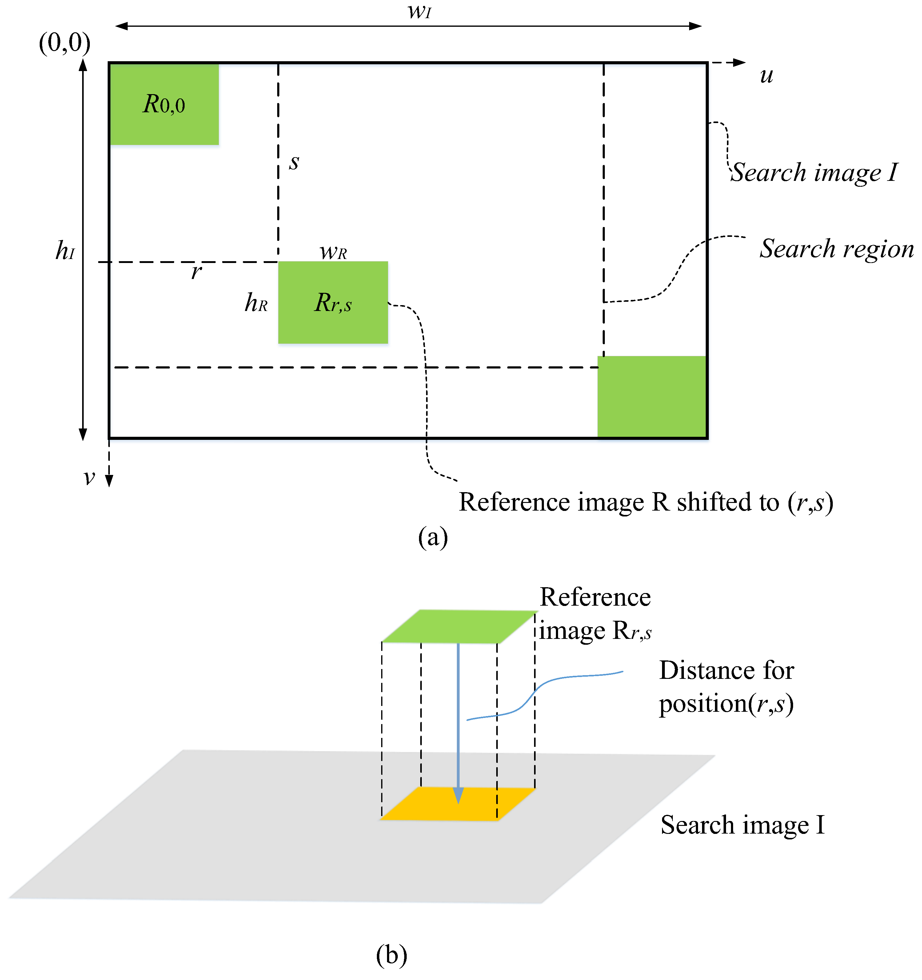
The cross-correlation function [39] can measure the similarity between different patterns and can be derived from template matching of gray-scale images. The basic principle is very simple. First, in the image to be searched, move the template image, measure the difference between the subimage of the image to be searched and the template image at each position, and then record the corresponding position when the similarity reaches its maximum. However, the actual situation is complex. For practical applications, an appropriate distance measurement method and the total distance difference for a highly similar match must be determined. As shown in Figure 1a, the search region is defined with the origin of the two images as the reference point, and the maximum search area is determined by the size of the image to be searched and the size of the template image.

Template matching in gray-scale images mainly involves finding the same or most similar position between the template image R and the subimage in the searched image, I. The following equation represents the template offset in the image searched by (r,s) units. A schematic of this is shown in Figure 1b.

$$R_{r,s}(u,v)=R(u-r,v-s)$$

(6)

The most important aspect of template matching is the similarity measurement function, which is robust to gray-scale and contrast changes. To measure the similarity between images, the distance d(r,s) between the reference template image and the corresponding subimage in the searched image after each translation (r,s) is calculated. Several basic measurement functions exist for gray-scale images: the sum of absolute differences, the maximum difference, and the sum of squared differences (SSD), as shown in Equations (7)–(9), respectively.

$$d_A(r,s)={\displaystyle \sum _{(i,j)\in R}\left|I(r+i,s+j)-R(i,j)\right|}$$

(7)

$$d_M(r,s)=\underset{(i,j)\in R}{\max }\left|I(r+i,s+j)-R(i,j)\right|$$

(8)

$$d_E(r,s)={\left[{\displaystyle \sum _{(i,j)\in R}{\left(I(r+i,s+j)-R(i,j)\right)}^2}\right]}^{1/2}$$

(9)

The SSD function is often used in statistics and optimization fields. To determine the best matching position for the reference image in the searched image, minimizing the SSD function is necessary. That is, Equation (10) reaches a minimum value.

$$\begin{array}{l}{d}_E^2(r,s)={\displaystyle \sum _{(i,j)\in R}{\left(I(r+i,s+j)-R(i,j)\right)}^2}\\ =\underset{A(r,s)}{\underbrace{{\displaystyle \sum _{(i,j)\in R}{I}^2(r+i,s+j)}}}+\underset{B}{\underbrace{{\displaystyle \sum _{(i,j)\in R}{R}^2(i,j)}}}-2\underset{C(r,s)}{\underbrace{{\displaystyle \sum _{(i,j)\in R}I(r+i,s+j)\cdot R(i,j)}}}\end{array}$$

(10)

where B is the sum of the squares of the gray-scale values of all the pixels in the reference template image. It is a constant (independent of r and s) and can be ignored when calculating the minimum SSD value. A(r,s) represents the sum of the squares of the gray-scale values of all the pixels in the subimage of the searched image at the (r,s) coordinate position. C(r,s) denotes the linear cross-correlation function of the searched image and the reference template image, and it can be expressed as

$$C(r,s)=\left(I\otimes R\right)\left(r,s\right)={\displaystyle \sum _{i=-\infty }^{\infty }{\displaystyle \sum _{j=-\infty }^{\infty }I(r+i,s+j)\cdot R(i,j)}}$$

(11)

When R and I exceed the boundary, their values are zero. Thus, the above formula can also be expressed as

$${\displaystyle \sum _{i=0}^{w_R-1}{\displaystyle \sum _{j=0}^{h_R-1}I(r+i,s+j)\cdot R(i,j)={\displaystyle \sum _{(i,j)\in R}I(r+i,s+j)\cdot R(i,j)}}}$$

(12)

Assuming that A(r,s) is a constant in the searched image, its value is negligible when calculating the best match position in the SSD; when C(r,s) reaches its maximum value, the reference template image and the subimage in the search image are most similar. Essentially, the minimum SSD value is obtained by calculating the maximum value of C(r,s).

2.2.2. Pattern Distribution-Based Loss Function for Two-Phase Core Image Reconstruction

The pattern distribution of the porous microstructure in the two-phase core images reflects their morphological characteristics. The loss function based on the pattern distribution measures the difference between the predicted and true values of the pattern distribution in the two images and is defined as follows:

$$L_{pattern}={\mathbb{E}}_{A~p(A),z~p(z)}{‖B_{pattern}-{\left(G\left(A,z\right)\right)}_{pattern}‖}_2^2$$

(13)

A pattern in an image is defined as data consisting of multiple points captured by a template. Taking the template as an example, the calculation process for the pattern distribution of a binary image is shown in Figure 2. Specifically, the following steps are involved:

• Scan across the image (via convolution) with the template to collect all occurrences of patterns Pat_i;
• Flatten each pattern to obtain its corresponding binary code and convert it to a decimal number PatNum_i;
• Count each pattern Pat_i that appears, obtain the number NUM(Pat_i), and normalize it to obtain the probability of each pattern P_i, defined as

  $$p_i={\displaystyle \frac{NUM\left(Pa{t}_i\right)}{N_{total}}}$$

  (14)

  where N_total represents the total number of patterns in an image. With a 3 × 3 template, 2⁹ = 512 possible patterns exist.

Figure 2. Schematic diagram for calculating the distribution of two-phase core image patterns.

Figure 2. Schematic diagram for calculating the distribution of two-phase core image patterns.

As shown in Figure 2, a 3 × 3 template is used to traverse the image in a raster path. The sum of all patterns is N_total. In this example, three patterns are taken. Flattening these patterns yields 000000000, 111111111, and 001110010. These patterns are converted to decimals. For example, the conversion process for the third pattern is 2⁰ × 0 + 2¹ × 1 + 2² × 0 + 2³ × 0 + 2⁴ × 1 + 2⁵ × 1 + 2⁶ × 1 +2⁷ × 0 + 2⁸ × 0 = 114. The number of patterns with a decimal value of 114 increases by 1. Finally, NUM(Pat_i)/N_total is the pattern density of a specific decimal value.

2.2.3. Construction of Physics Statistical Descriptor—Gray-Scale Pattern Density Function

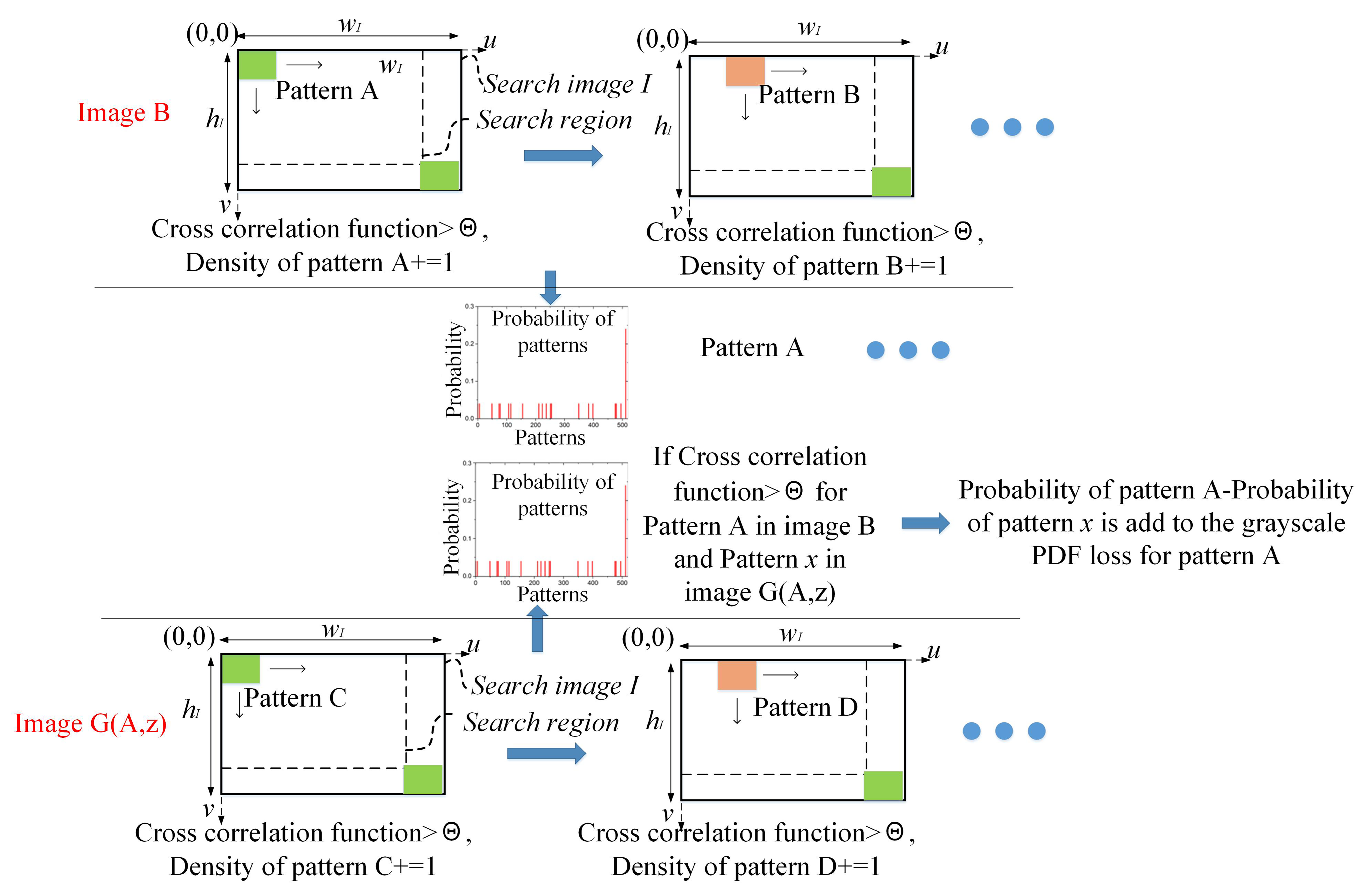
The pattern distribution-based loss function for two-phase core images (Section 2.2.2) encodes different patterns and compares their distribution across two binary core images. However, for a gray-scale core image template such as the 5 × 5 template, the value range of each pixel is 0–255 and the total number of patterns is large, which makes it impossible to encode and construct a pattern density function based on it. The MSE is used as a metric to measure the difference between two patterns. The cross-correlation function is a more suitable metric for gray scale patterns. Therefore, a new physics statistical descriptor—the gray-scale pattern density function—is constructed and proposed through a cross-correlation function. Its schematic diagram is shown in Figure 3, and the formulas are shown in Equations (15)–(17).

Here, Image B is the target system image and G(A,z) is the image generated by the generator. Images B and G(A,z) were scanned, the patterns were traversed, and the cross-correlation function between the patterns was calculated to construct the gray-scale pattern density functions, B_pattern(i₁,j₁) and G(A,z)_pattern(i₁,j₁). On this basis, for each pattern (Pattern A, for example) in the gray-scale pattern density function B_pattern(i₁,j₁), if the cross-correlation function >Θ between Pattern A and Pattern x in image B, the difference between the probabilities of Patterns A and Pattern x is added to the gray-scale PDF loss for Pattern A.

$$B_{pattern}(i_1,j_1)={\displaystyle \sum _{i=i_1}^{w_R-1}{\displaystyle \sum _{j=j_1}^{h_R-1}B(r+i,s+j)\cdot R(i_1,j_1)\hspace{1em}}}{i}_1\in (0, w_R-1),j_1\in (0, h_R-1)$$

(15)

$$G{\left(A,z\right)}_{pattern}(i_1,j_1)={\displaystyle \sum _{i=i_1}^{w_R-1}{\displaystyle \sum _{j=j_1}^{h_R-1}G\left(A,z\right)(r+i,s+j)\cdot R(i_1,j_1)\hspace{1em}}}{i}_1\in (0, w_R-1),j_1\in (0, h_R-1)$$

(16)

$$L_{GrayscalePDF}={\mathbb{E}}_{A~p(A),z~p(z)}‖B_{pattern}\cdot {\left(G\left(A,z\right)\right)}_{pattern}‖$$

(17)

2.3. PSDI-DISTS Metric

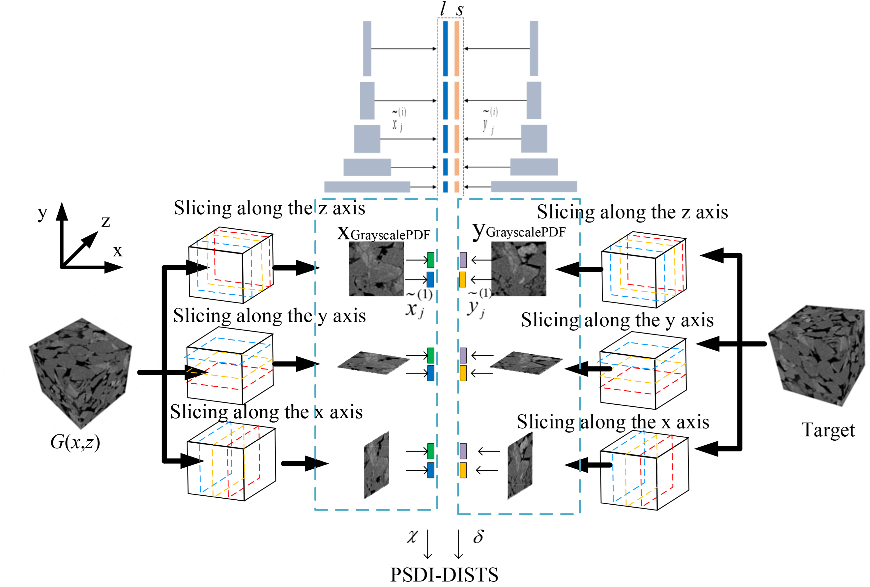
DISTS unifies structure and texture similarities, is robust to mild geometric distortions, and performs well in texture-relevant tasks. However, not only does the gray-scale core image reconstruction task require that the generated image has texture similarity with the target image but the subsequent generated image also needs to be used to simulate physical properties such as seepage characteristics. Therefore, the addition of a PSD is crucial. Simultaneously, the 3D gray-scale core structure must be reconstructed; therefore, it is necessary to perform a similarity evaluation in the x, y, and z directions. Accordingly, this study proposes and constructs a PSDI-DISTS metric. Two-dimensional slices are extracted from I_3D along the z/y/x-axis independently (i.e., I_2Dxy ∈ R^ℎH×wH, I_2Dxz ∈ R^ℎH×dH, and I_2Dyz ∈ R^wH×dH). The final metric is formed by combining the three directions, and its formula is shown in Equations (18)–(21). The schematic diagram of the PSDI-DISTS metric is shown in Figure 4.

$$\mathrm{PSDI-DISTS}({\mathrm{X}}_{2Dxy},{\mathrm{Y}}_{2Dxy})=\chi \cdot \left\{{\displaystyle \sum _{l=1}^L[{\alpha }_l\cdot S_{struct}^{(l)}({\mathrm{X}}_{2Dxy},{\mathrm{Y}}_{2Dxy})+{\beta }_l\cdot S_{texture}^{(l)}({\mathrm{X}}_{2Dxy},{\mathrm{Y}}_{2Dxy})]}\right\}+\delta \cdot L_{GrayscalePDF}({\mathrm{X}}_{2Dxy},{\mathrm{Y}}_{2Dxy})$$

(18)

$$\mathrm{PSDI-DISTS}({\mathrm{X}}_{2Dxz},{\mathrm{Y}}_{2Dxz})=\chi \cdot \left\{{\displaystyle \sum _{l=1}^L[{\alpha }_l\cdot S_{struct}^{(l)}({\mathrm{X}}_{2Dxz},{\mathrm{Y}}_{2Dxz})+{\beta }_l\cdot S_{texture}^{(l)}({\mathrm{X}}_{2Dxz},{\mathrm{Y}}_{2Dxz})]}\right\}+\delta \cdot L_{GrayscalePDF}({\mathrm{X}}_{2Dxz},{\mathrm{Y}}_{2Dxz})$$

(19)

$$\mathrm{PSDI-DISTS}({\mathrm{X}}_{2Dyz},{\mathrm{Y}}_{2Dyz})=\chi \cdot \left\{{\displaystyle \sum _{l=1}^L[{\alpha }_l\cdot S_{struct}^{(l)}({\mathrm{X}}_{2Dyz},{\mathrm{Y}}_{2Dyz})+{\beta }_l\cdot S_{texture}^{(l)}({\mathrm{X}}_{2Dxy},{\mathrm{Y}}_{2Dxy})]}\right\}+\delta \cdot L_{GrayscalePDF}({\mathrm{X}}_{2Dyz},{\mathrm{Y}}_{2Dyz})$$

(20)

$$\mathrm{PSDI-DISTS}(\mathrm{X},\mathrm{Y})=\mathrm{PSDI-DISTS}({\mathrm{X}}_{2Dxy},{\mathrm{Y}}_{2Dxy})+\mathrm{PSDI-DISTS}({\mathrm{X}}_{2Dxz},{\mathrm{Y}}_{2Dxz})+\mathrm{PSDI-DISTS}({\mathrm{X}}_{2Dyz},{\mathrm{Y}}_{2Dyz})$$

(21)

3. TFCGAN for Three-Dimensional Gray-Scale Core Image Reconstruction

3.1. Main Architecture of the TFCGAN

Figure 5 shows the network architecture of the generator G used to reconstruct a 128³-size image in this study. The input is Gaussian noise N(z) and a 2D image, and the output is a 3D structure. As shown in the figure, the network architecture was based on a classic U-Net. Notably, to obtain a faster inference speed in the previous algorithm, the generation network used a 2D convolution and a 2D transposed convolution. The convolution layer fusing channel information was added to the last layer. Both 3D convolution (Conv3D) and 3D transposed convolution (ConvT3D) were used to better capture 3D spatial information. However, 3D operations cause greater difficulties in training the network and easily result in insufficient GPU memory. To address this problem, this study omitted the final channel fusion process because 3D (transposed) convolution is an operation performed in three dimensions, which can effectively fuse the information between channels. Therefore, it was designed such that the image input into generator G was downsampled to a size of 2 × 2 to reduce the number of network parameters, save memory, and accelerate network convergence. This article uses a GeForce RTX 1080 Ti graphics card (11 GB of GPU memory, NVIDIA Corporation, Santa Clara, CA, USA). In early testing, with a batch size of 1, training 128 × 128 size samples required approximately 7 GB of GPU memory. Downsampling images to 2 × 2 in generator G has a minimal impact on accuracy, but this strategy can reduce network parameters by approximately 30%, saving GPU memory and accelerating network convergence.

This study used a deep-gray padding technique while processing the input image to fill in the input image with the target image size. Thus, the network learned the mapping relationship between the 3D input and 3D output. Compared to the original learning of the mapping relationship from 2D to 3D images, the learning of this network was easier. This is because after adopting deep-gray padding technology, the input and target are set as two 3D bodies with equal structures, which is more convenient when using 3D convolution for feature extraction. The principle of deep-gray padding is illustrated in Figure 5.

The proposed model is illustrated in Figure 6. As shown in the figure, the algorithm uses the classic BicycleGAN model [40] as its basic framework. The core idea is to explicitly establish a connection between the noise and the target. Compared to the Pix2Pix model [41], the BicycleGAN model introduces an additional encoder. Its two subnetworks, cVAE-GAN and cLR-GAN, serve different functions, as described below.

The cVAE-GAN model can be regarded as a reconstruction of target B. The entire network implements an autoencoder function; that is, target B is the input of cVAE-GAN, and the output is an approximate or equivalent reconstruction value $\hat{\mathit{B}}$($\mathit{B}\to \mathit{z}\to \hat{\mathit{B}}$). The cLR-GAN model realizes the reconstruction of noise N(z). That is, noise N(z) is the input of cLR-GAN, and the approximate value $\hat{\mathit{z}}$($\mathit{z}\to \widehat{B}\to \hat{\mathit{z}}$) is the output of the network. The network consists of a generator G and discriminator D. During the training process, generator G receives input A and noise N(z) (usually Gaussian noise) and outputs a predicted value $\hat{\mathit{B}}$. The discriminator evaluates the quality of the predicted value; that is, the difference between $\hat{\mathit{B}}$ and B is calculated using the loss functions PSDI-DISTS and L₁.

3.2. Balanced Training Strategy Integrating L₁ and PSDI-DISTS Losses

By introducing the PSDI-DISTS loss, the textural similarity between the reconstructed 3D structure and target can be maintained. However, experiments showed that if only the PSDI-DISTS loss is used, the generator becomes lazy.

In this case, despite the 2D gray-scale core image chosen as the input, the generator tended to find a known 3D structure from the training set as the reconstruction result. This is because the structure directly obtained by the generator from the known training set also satisfied the textural and physical property similarities required for the PSDI-DISTS loss. Therefore, a balanced training strategy integrating L₁ and PSDI-DISTS losses was introduced. In the early stage of training, the L₁ loss was given a larger weight; therefore, the generator network realized that the results obtained from the known training set cannot deceive the discriminator. Thereafter, the weight of the L₁ loss was reduced to a level equivalent to that of PSDI-DISTS. For TFCGAN, at each timepoint when iterating N epochs, the loss weight $\tau$ of the loss function L₁ was decayed according to the decay factor $\gamma$; that is, ${\tau }_{\mathit{new}}=\gamma {\tau }_{\mathit{old}} \left(\mathrm{if} {\tau }_{\mathit{old}}>\sigma \right)$ (${\tau }_{\mathit{new}}$ and ${\tau }_{\mathit{old}}$ represent the new L₁ loss weight and the old L₁ loss weight, respectively). In the initial state, $\tau$ = 100, $\sigma$ = 10, and $\varsigma$ = 10. The final loss and weight decay are given according to Equations (22) and (23).

$$L_{\mathit{total}}=\sigma \mathrm{PSDI-DISTS}(\mathrm{X},\mathrm{Y})+\varsigma L_{GAN}+\tau L_1$$

(22)

$${\tau }_{\mathit{new}}=\gamma {\tau }_{\mathit{old}} \left(\mathrm{if} {\tau }_{\mathit{old}}>\varsigma \right)$$

(23)

In summary, L₁ loss describes the sum of the point-to-point pixel value differences between the generated structure and the target system. Initially, the L₁ loss is heavily weighted. At this stage, if the generator directly takes samples from the training set, even though these samples have great texture and physical property similarity with the target system, the sum of the pixel value differences is large due to the different structures, making it difficult to deceive the discriminator. This forces the generator to learn realistic textural and physical statistical properties rather than directly taking samples from the training set. Later on in training, the L₁ loss weight decays to a degree comparable to PSDI-DISTS, jointly constraining model learning.

3.3. Dataset Establishment and Parameter Settings

To test the reconstruction results, we used the real core CT images for verification. In the experiment, the test objects are core samples from the supplementary materials of the paper “Segmentation of digital rock images using deep convolutional autoencoder networks” by Sadegh Karimpouli and Pejman Tahmasebi (3DμCT image of Berea sandstone with a size of 1024 × 1024 × 1024 voxels and a resolution of 0.74 μm). From this 3DμCT image, the authors randomly cut out 3D cubes of 128 × 128 × 128 voxels to build a dataset. A total of 600 samples were created, of which 70% were used as the training set and 30% were used as the test set. Each sample was composed of a 2D image (input) and a 3D structure (target).

The key algorithm parameters include noise reconstruction loss weights λ_latent, discriminator loss weights λ_dis, learning rates for generator G and D, batch size, and number of iterations (epoch). Experiments have shown that heterogeneous training images are unstable. The network collapses easily in the later stage of the iterative process, and there is no convergence. To address this problem, this study adopted the learning rate decay strategy; that is, the learning rate was decayed according to the decay factor γ at every N epoch (step), so lr_new = γlr_old. The parameter settings are listed in

Table 1. Main parameters.

Parameter	Value
Weight of the noise (${\lambda }_{\mathrm{latent}}$)	0.5
Weight of the discriminator (${\lambda }_{\mathrm{dis}}$)	$1$
Initial learning rate of G and D	2 × 10−4
Step size of learning rate decay (step)	20
Learning rate decay factor ($\gamma$)	0.8
Batch size	1
Epoch	200

. Similarly, to fully verify the stability and accuracy of the algorithm, we reconstructed the same image 20 times and analyzed the visual contrast and statistical average.

The experiments were run on an Intel i7-6700k system, with 16 GB DDR3 RAM, Nvidia GTX 1080 GPU, and an Ubuntu 16.04 operating system. A core image of size 128³ pixels was reconstructed in 0.5 s. The reconstruction time increased with the size of the network input data. For a core image of size n³ in terms of the amount of data, n³ = 128³ × (n/128)³. Thus, the reconstruction time would be approximately (n/128)³ times the reconstruction time of the 128³ size core image, that is, (n/128) 3 × 0.5 s.

The Pix2Pix model suffers from a certain degree of mode collapse. Mode collapse refers to the network’s limited generative capabilities, often only generating a small number of modes (or even a single mode). Specifically, when the input remains unchanged and only the input noise is varied, the output remains almost unchanged. Essentially, this is because noise N(z) is only added to the input of the network, without explicitly establishing a connection between the noise N(z) and the output.

The TFCGAN proposed in this paper uses BicycleGAN as its basic architecture. Its main purpose is to explicitly establish a connection between noise and target values. In the cLR-GAN model of BicycleGAN, first, the input A and Gaussian noise N(z) are fed into the generator to obtain the predicted value $\widehat{B}$. Then, $\widehat{B}$ is fed into the encoder E to obtain the noise distribution $\widehat{z}$. The loss function L₁ measures the difference between the noise N(z) and $\widehat{z}$. This makes TFCGAN training more stable. In the experiments, the generator and discriminator losses of TFCGAN reached a stable state after 120 epochs.

4. Results and Discussion

This paper proposes to combine the DISTS metric [37] with the physics statistical descriptor (gray-scale pattern density function) designed by the authors and also proposes the PSDI-DISTS metric, so that the reconstructed structure constrained by this method maintains good texture characteristics while having physical and statistical characteristics similar to the target system. As can be seen from [37], DISTS has an advantage in comparison with other texture metrics. Therefore, this paper does not use or compare the combination of the physics statistical descriptor and metrics other than DISTS. Since this paper belongs to the field of gray-scale core image 3D reconstruction, we focus on comparing PSDI-DISTS-based TFCGAN with other gray-scale core reconstruction algorithms and verify the advantages of PSDI-DISTS and related TFCGAN models in terms of the statistical characteristics, texture characteristics, and seepage characteristics of the gray-scale core image structure reconstructed.

4.1. CPGAN

The cascaded progressive GAN (CPGAN) algorithm [31] can also be used to reconstruct gray-scale core images. In this study, it was used as a comparative algorithm to assess the performance of multimineral core reconstruction.

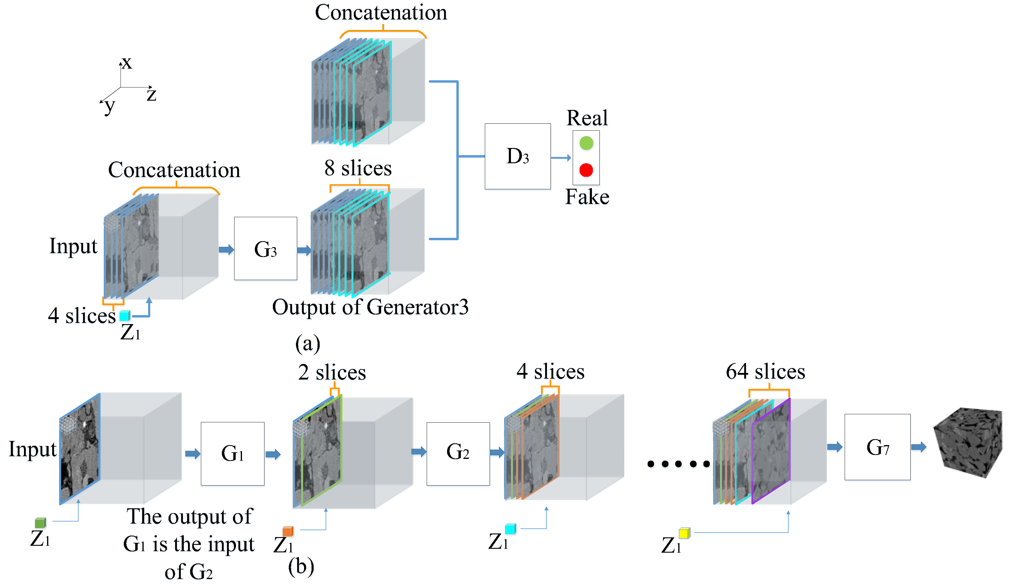
CPGAN converts the 2D-to-3D gray-scale core image reconstruction problem into a step-wise reconstruction problem. The reconstruction of the first network node can be regarded as a 2D-to-2D image reconstruction, and the reconstruction of subsequent nodes can be regarded as 3D-to-3D image reconstruction, thereby reducing the information difference between the input and output during reconstruction.

In the training stage, in the iteration of the nth single-layer node network (for a reference image of 128 × 128 pixels, n ranges from 1 to 7), the known information is 2n − 1 consecutive images in the CT sequence, and the images to be reconstructed are the 2n − 1 images immediately following them in the CT sequence. In the reconstruction stage, the k generators trained above are cascaded (k = 7 when the reference image size is 128). The input is a 3D volume, in which the 2D gray-scale core reference image to be reconstructed is the first layer, and the other layers are filled with pixels with a gray-scale value of 127. This 3D volume is first sent to the first layer of the CPGAN network, and its output is used as the input for the next network layer. The above operation reconstructs 2k images from the original reference image. By stacking these 2k images, the entire 3D structure can be reconstructed. The training stage of the third-layer node network of the CPGAN and a schematic diagram of the entire reconstruction stage are shown in Figure 7a and b, respectively.

4.2. Comparison of Experimental Results

4.2.1. Reconstruction Results

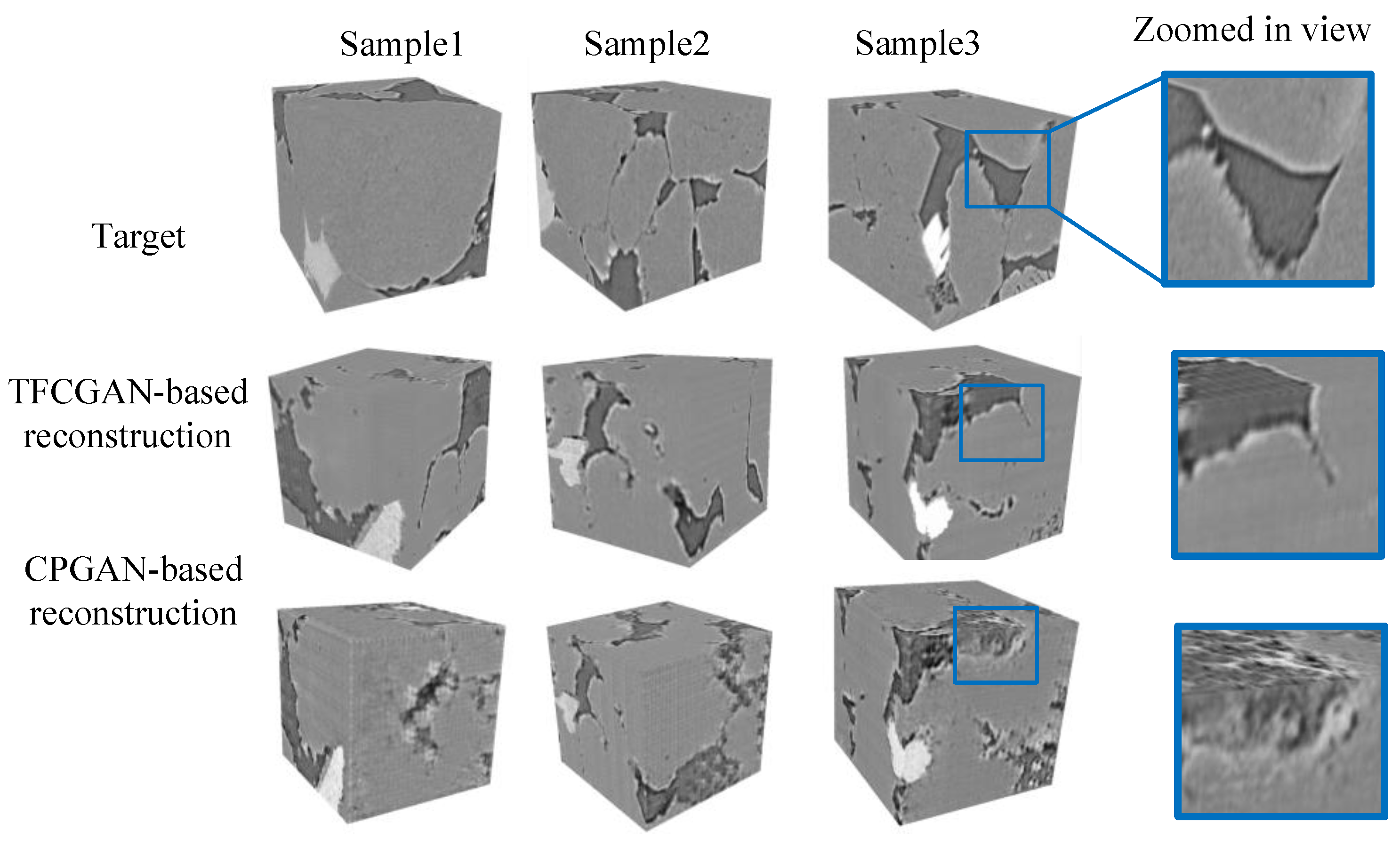
Training and reconstruction were carried out using the materials described in Section 3.3. Figure 8 shows a schematic of the three 128 × 128 × 128 target samples and the structures reconstructed by the TFCGAN and CPGAN.

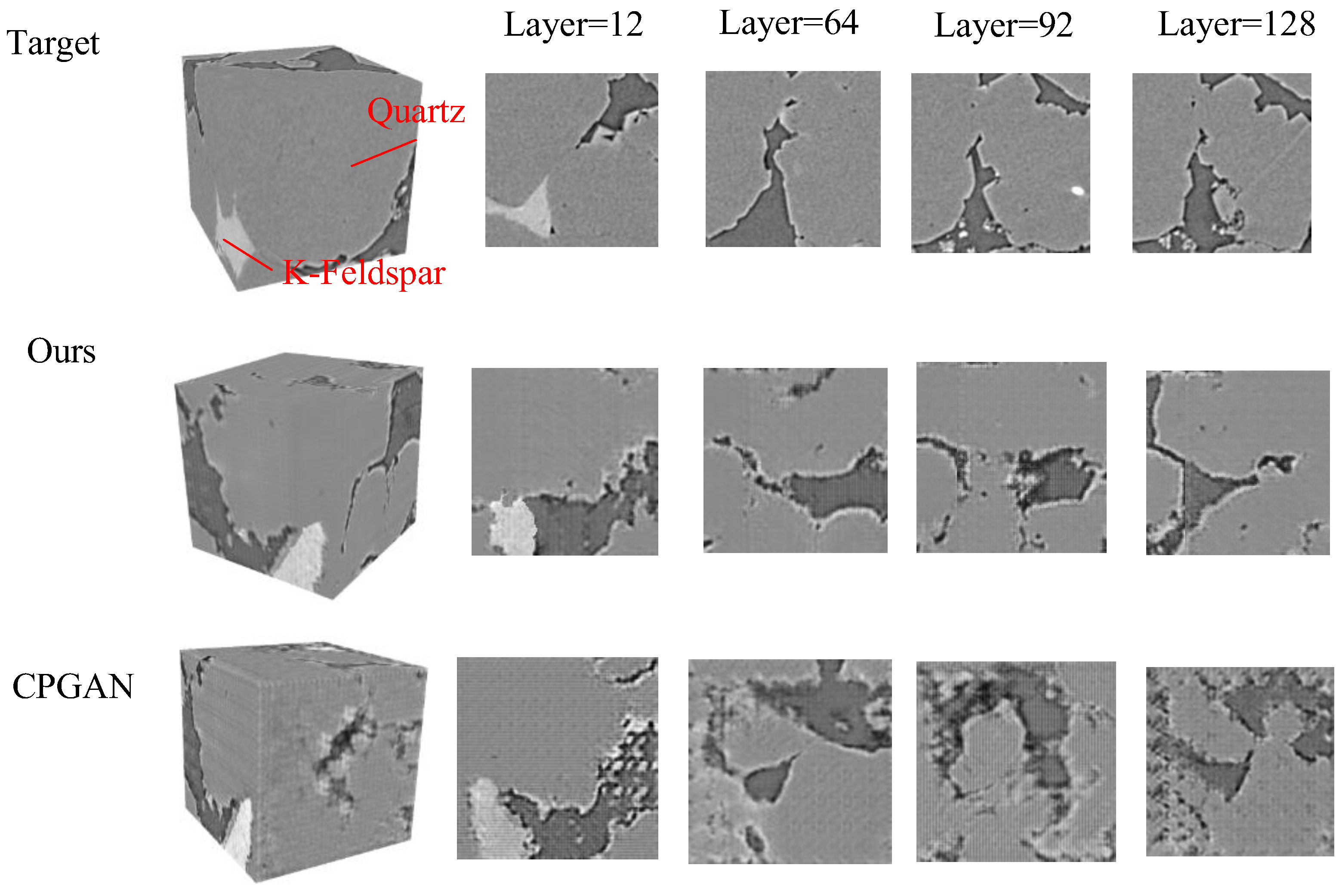
Based on the visual effects of the three groups of samples shown in Figure 8, the texture features of the structure reconstructed by the TFCGAN algorithm were closer to those of the target system. This is because the TFCGAN algorithm uses the PSDI-DISTS metric as a constraint for model training, thereby controlling the textural characteristics of different mineral components to be close to the target system during the training process. In contrast, the CPGAN algorithm reconstructs structural texture features with certain textural blurring. This is because although the CPGAN algorithm uses a step-wise reconstruction strategy to reduce the difficulty of reconstruction, the solution space for the reconstruction of 2D–3D mineral core images is complex. As the reconstruction proceeded, the 3D structure to be reconstructed gained a higher uncertainty, and the CPGAN model exhibited textural blurring when determining these structures. In general, a higher-order optimization criterion, such as the TFCGAN, must be adopted to reconstruct its structure accurately.

On this basis, for the target system and the reconstruction structures of the different algorithms shown in Figure 9, to further compare the reconstruction effects of the multimineral core images, we used different quantitative criteria to analyze the reconstruction results.

4.2.2. Two-Point Correlation Function, S₂(r), for Different Minerals

The two-point correlation function, S₂(x₁,x₂), is commonly used to characterize porous media. It represents the correlation of the spatial distribution of two points x₁ and x₂, that is, the probability that the two points belong to the same target mineral. This is defined as follows:

$$S_2\left({\mathbf{x}}_1,x_2\right)=〈I\left(x_1\right)I\left(x_2\right)〉$$

(24)

where I(x) is the indicator function and the brackets $〈\cdot 〉$ represent the statistical mean.

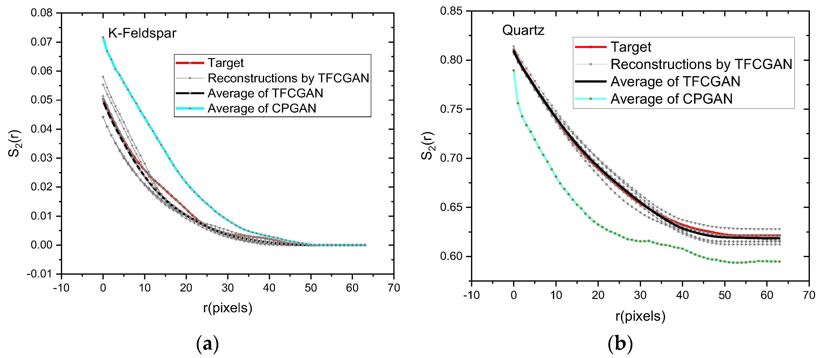
Here, we compare the ACF of the two mineral components, K-Feldspar and Quartz, in the three-dimensional structure reconstructed by the TFCGAN and CPGAN algorithms in Figure 9 with the ACF of the corresponding components in the target system. The statistical curve diagram is shown in Figure 10. As shown in the figure, the K-Feldspar and Quartz S₂(r) curves of the ten reconstructions generated by the TFCGAN and their averages were consistent with those of the target system. However, the ACF curves of the different mineral components of the structure reconstructed by the CPGAN algorithm deviated significantly from those of the target system. That is, the CPGAN overestimated the proportion of K-Feldspar minerals in the target system and underestimated the proportion of Quartz. This is because PSDI-DISTS renders the TFCGAN model more complex and powerful. However, the data distribution of the 3D multimineral core structure itself is complex, and the solution space is a high-dimensional solution space. Thus, the TFCGAN is suitable for 2D–3D gray-scale core reconstruction. In contrast, the complexity of the 3D multimineral core data distribution exceeded the expression ability of the CPGAN, resulting in the phenomenon shown in the figure.

Pearson’s correlation coefficients for the ACF curves were calculated and compared, indicating the degree of correlation between two variables on a scale from −1 to 1. The correlation coefficient approaches 1 when the positive correlation is stronger. The formula for Pearson’s correlation coefficient is shown in Equation (25).

$$r_{xy}={\displaystyle \frac{{\displaystyle \sum _{i=1}^n\left(x_i-\overline{x}\right)\left(y_i-\overline{y}\right)}}{\sqrt{{\displaystyle \sum _{i=1}^n{\left(x_i-\overline{x}\right)}^2}}\sqrt{{\displaystyle \sum _{i=1}^n{\left(y_i-\overline{y}\right)}^2}}}}$$

(25)

where x_i and y_i are the observed values of two variables. $\overline{x}$ and $\overline{y}$ are the means. The numerator denotes the covariance, which measures whether the trends in the two variables are consistent. The denominator denotes the product of the standard deviations of the two variables, which is used to standardize the results. This formula evaluates the strength and direction of the correlation between two variables using a standardized covariance. It describes how when one variable increases, the other variable increases or decreases, and the consistency of the change.

For K-Feldspar, the Pearson correlation coefficients of the ACF curves were 0.99786 and 0.99441 for the TFCGAN and CPGAN, respectively. For Quartz, the coefficients were 0.99943 and 0.98007 for the TFCGAN and CPGAN, respectively. The quantitative analysis results showed that the TFCGAN reconstruction results were more consistent with the statistical characteristics and distribution of the different mineral components in the target system.

Based on this, the standard error was used to further quantify the ACF curve. The standard error is a measure of the difference between the measured value and the target, which is also known as the mean square error. Suppose the errors of n measured values are ξ₁, ξ₂, ξ₃, …, ξ_n; then, the standard error, σ, of this set of measured values can be expressed as follows:

$$\sigma =\sqrt{{\displaystyle \frac{{\xi }_1^2+{\xi }_2^2+......+{\xi }_n^2}{n}}}=\sqrt{{\displaystyle \frac{{\displaystyle \sum {\xi }_i^2}}{n}}}$$

(26)

Based on the formula above, for K-Feldspar, the standard error of the ACF value between the average of the TFCGAN reconstructions and the target is 0.00137. The corresponding value for the CPGAN is 0.01009. For Quartz, the standard errors of the ACF curves are 0.00240 for the TFCGAN and 0.042 for the CPGAN. These results reveal that the proposed model can reconstruct K-Feldspar and Quartz more accurately. Furthermore, it results in better reconstruction quality and higher consistency with the testing target compared to the CPGAN.

4.2.3. Comparison of Learned Perceptual Image Patch Similarity (LPIPS)

Textural similarity measurement is key for object recognition and scene understanding. In recent years, it has played a significant role in constructing training losses for image synthesis tasks using VGG networks. LPIPS is an image texture similarity evaluation metric that uses a VGG network based on deep learning. By learning the perceptual relevance of an image’s content, LPIPS provides an image quality evaluation method that is more in line with the texture characteristics of human visual perception.

The LPIPS flowchart is shown in Figure 11. Two inputs are sent to the neural network F (VGG is used here) for feature extraction. The output of each layer is activated, normalized, and recorded as ${\hat{\mathrm{y}}}^l,{\hat{\mathrm{y}}}_0^l\in R^{H_l\times W_l\times C_l}$, and then the L₂ distance is calculated for ${\hat{\mathrm{y}}}^l$ and ${\hat{\mathrm{y}}}_0^l$ after multiplying together the weights of the w layers as follows:

$$d(x,x_0)={\displaystyle \sum _l\frac{1}{H_l{W}_l}}{{\displaystyle \sum _{h,w}‖w_l\odot ({\hat{\mathrm{y}}}_{hw}^l-{\hat{\mathrm{y}}}_{0hw}^l)‖}}_2^2$$

(27)

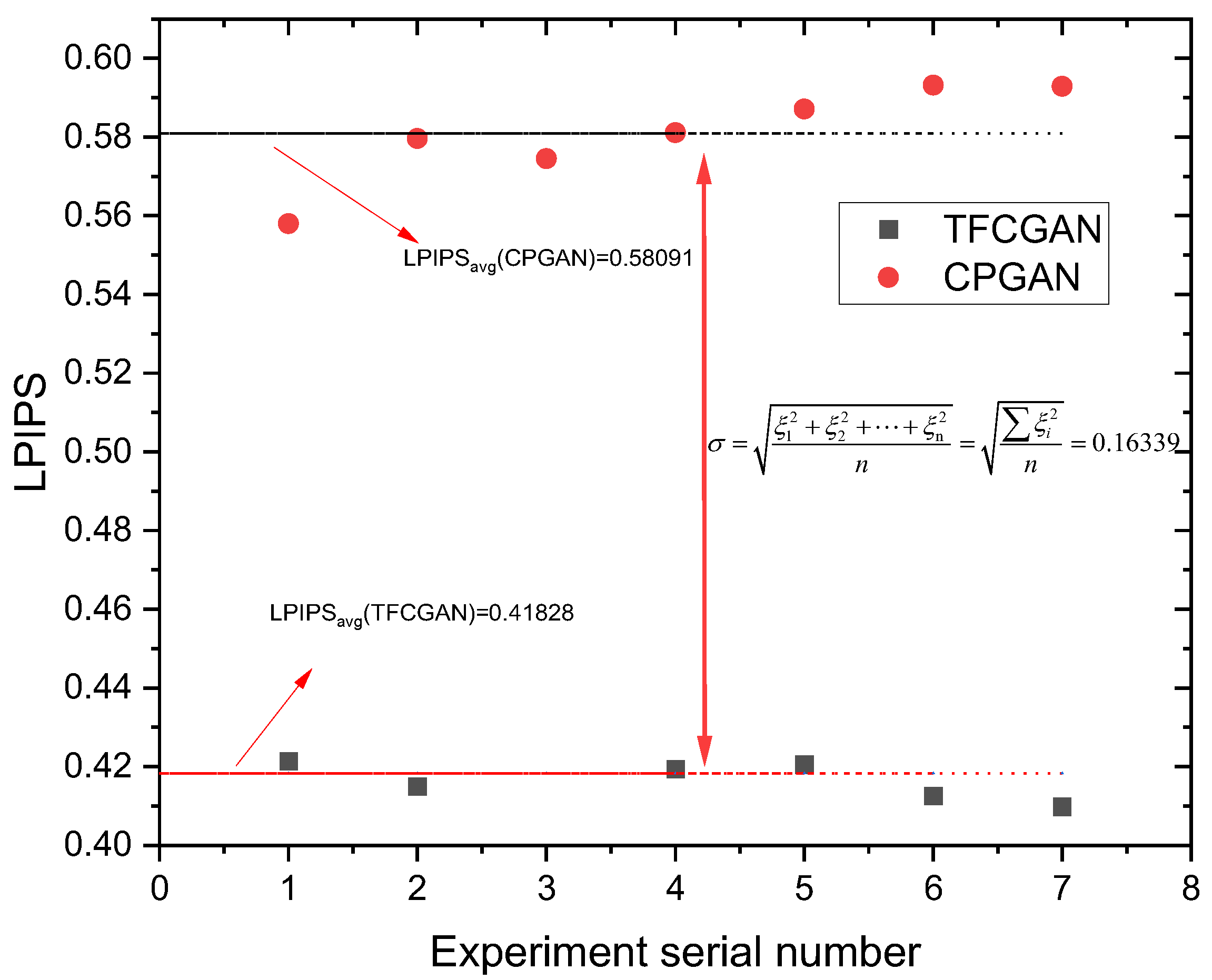
For the target in Figure 9, we conducted seven sets of repetitive reconstruction experiments using the TFCGAN and CPGAN algorithms and calculated the LPIPS between each set of experimental results and the target. The corresponding schematic is shown in Figure 12. The LPIPS value of the 3D structure reconstructed using the TFCGAN and the corresponding target 3D structure fluctuates around 0.41828, with a standard deviation of 0.00471. For the CPGAN, the DISTS value fluctuates around 0.58091 with a standard deviation of 0.01225. This shows that the fluctuations in the LPIPS values calculated by the two algorithms were very small, thus proving the stability of the two algorithms. However, the mean LPIPS of the TFCGAN is considerably smaller than that of the CPGAN, and the standard error between them reaches 0.16339, which is 39.06% of the TFCGAN LPIPS mean. Therefore, compared with that reconstructed by the CPGAN, the 3D structure reconstructed by the TFCGAN can better maintain the textural characteristics of the reconstructed structure.

4.2.4. Comparison of Flow Velocity Field and Effective Permeability

The aim of 3D reconstruction is to use the reconstructed structure to analyze seepage and other physical characteristics [42,43,44,45,46,47,48,49,50,51,52,53]. To further analyze the reconstruction results shown in Figure 9, this section compares the flow velocity field and effective permeability. We used the PUMA V3 open-source analysis tool developed by Ferguson and Semeraro [54,55].

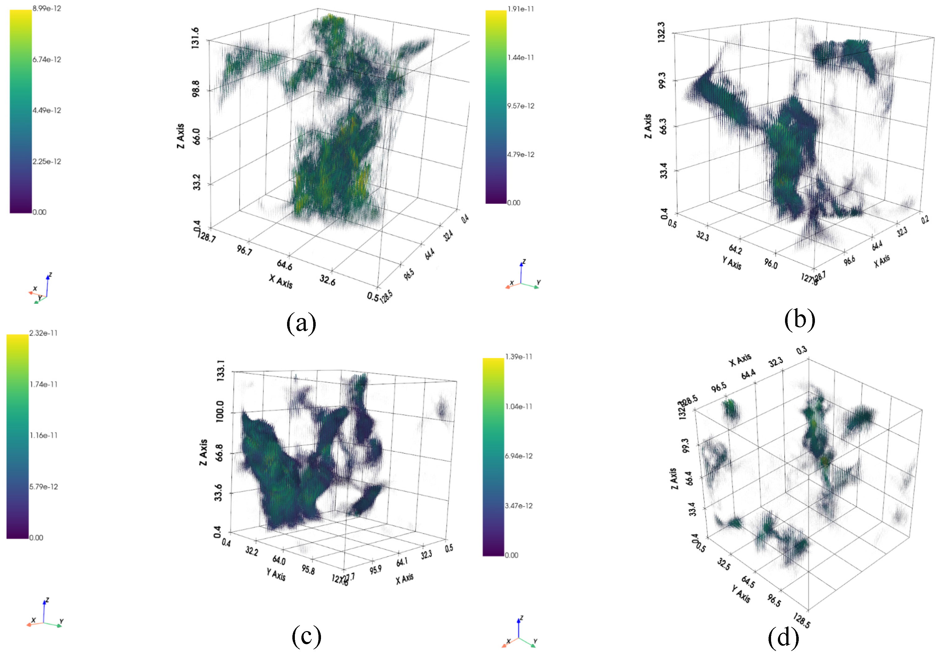
We used one randomly selected reference image from the target in Figure 9 to reconstruct the 3D multimineral core using the TFCGAN and CPGAN. In addition, a binarized reference image was used to reconstruct the binary core using BicycleGAN. The flow velocity fields of all the reconstructed structures and that of the target were calculated using PUMA V3, as shown in Figure 13. As shown in the figure, the velocity field of the structure reconstructed using the TFCGAN algorithm is closer to that of the target system, whereas the CPGAN algorithm overestimates the velocity field of the target system, and the binary core image reconstructed using BicycleGAN underestimates the velocity field. This is because the velocity field is closely related to the proportions and distributions of various mineral components and pore phases. Because of the constraints of the PSDI-DISTS metric, the reconstructed structure of the TFCGAN algorithm model is more similar to the mineral composition of the target system.

However, the CPGAN cannot model the high-dimensional data distribution of the target. Figure 9 shows that the proportions of K-Feldspar and the pore phase increase and the proportion of Quartz decreases. Therefore, the flow velocity field of the CPGAN algorithm was overestimated. In contrast, the binary cores only model the pore phase, whereas the other mineral phases are uniformly classified as rock phases. However, in reality, different mineral components grow differently in a 3D system, which affects the development of the pore and final flow fields. The difference between the velocity fields of the binary core image and the target system also confirms the necessity of multimineral core image reconstruction from another perspective.

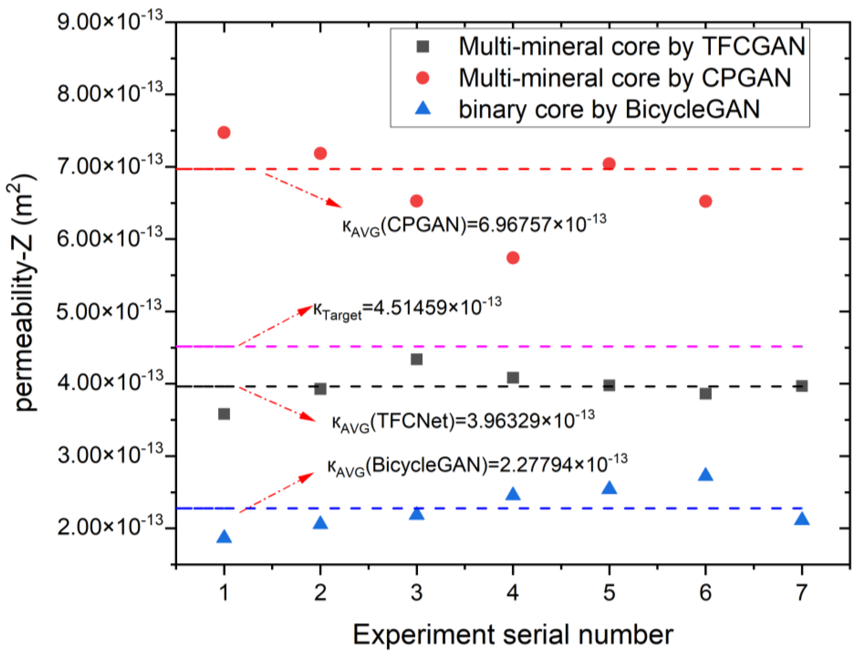
Based on this, the effective permeabilities of the different structures were computed using the minimal residual method iterative solver, as shown in Figure 14.

Through calculations, the standard error between the effective permeability of the 3D structure reconstructed by the TFCGAN and the target was 0.58991 × 10⁻¹³ m², and the corresponding values for the CPGAN and the binary core constructed by BicycleGAN were 2.56515 × 10⁻¹³ m² and 2.25388 × 10⁻¹³ m². The effective permeability of the target is similar to that of the reconstructed TFCGAN structure. This demonstrates that the TFCGAN can better reproduce the connectivity characteristics of the target system and therefore has more similar seepage characteristics.

As described in the original manuscript, a total of 600 samples were created for this experiment, of which 70% were used as the training set and 30% were used as the test set. Each sample was composed of a 2D image (input) and a 3D structure (target). There was no overlap between the training and test data. For example, in the samples in Figure 8 and Figure 9 of the manuscript, the input 2D slice is the leftmost section of the 3D structure, which did not appear in the previous training set. Subsequent quantitative analysis, including statistical characteristic indicators such as the two-point correlation function, the texture characteristic indicator LPIPS, and seepage characteristics, demonstrated that the reconstructed structure can reconstruct the target system well. This indicates that the model does not show significant overfitting.

5. Conclusions

The author designed the gray-scale pattern density function through the cross-correlation function and integrated it with the DISTS assessment metric to propose a new physics statistical descriptor-informed deep image structure and texture similarity (PSDI-DISTS) metric. In addition, this study employed the PSDI-DISTS metric as a loss function of the GAN and proposed the TFCGAN model for the reconstruction of gray-scale core images. Reconstruction results using the TFCGAN model and seepage simulation showed that the reconstruction results can maintain the texture characteristics of the target system and lead to similar seepage characteristics, thus proving the effectiveness of the proposed algorithm.

The algorithm described in this paper focuses on digital core 3D reconstruction. This involves reconstructing a 3D structure from a single 2D gray-scale core slice image. This reconstructed 3D structure is statistically and morphologically similar to the target 3D structure and can be used to analyze physical properties such as seepage, thereby guiding real-world petroleum geology research. Therefore, in answer to the reviewer’s question, the resolution of the input 2D image determines the resolution of the reconstructed 3D structure; 3D reconstruction itself does not improve resolution. Super-resolution reconstruction of 2D or 3D digital core images is also a separate research area. For related research, readers can refer to the following literature [56].

Although the TFCGAN algorithm effectively reconstructed the gray-scale core images, some problems remain, for example, the combination of neural networks and conventional methods. Significant progress has been made in recent years in terms of the accuracy of the 3D image reconstruction of cores. However, progress in terms of reconstruction speed has been slow, which could be because traditional reconstruction algorithms achieve reconstructions based on iterative processes. Although 3D reconstruction methods based on GPU or multithreading exist, there has been no change to the iterative reconstruction mechanism. Deep learning technology has the advantages of automatic feature extraction and faster inference speed. Recently, it has played an important role in image processing, video classification, and other fields. Therefore, the potential of deep learning to replace the iterative reconstruction mechanism in traditional algorithms and improve the reconstruction speed is worth considering.

In addition, although neural network-based approaches play an important role in various fields, we cannot completely neglect the development of traditional methods and pursue neural networks. Neural network methods are not omnipotent. If some prior information such as core porosity, pattern, shape distribution, and interlayer constraint information is incorporated into deep learning models as constraints or loss functions and if features described in the traditional method, such as a set of patterns in multipoint geostatistics, are utilized, the quality of reconstruction can be further improved. Therefore, for other specific problems, such as texture synthesis, image restoration, and super-resolution reconstruction, combining the different advantages of traditional and neural network methods is an important research direction.

Few-shot learning: The high cost of core scanning and the unique characteristics of some cores can result in a small number of collected samples. This poses challenges for learning-based methods, especially neural network methods, and further complicates subsequent computation and analysis. Transfer learning can be used to address this issue. The core idea behind transfer learning is to first train the neural network on a larger dataset, allowing it to find a general method for extracting features. Then, based on the specific problem being solved, targeted fine-tuning can be performed using certain prior information. Therefore, how to pre-train the neural network to perform small-shot learning based on specific problems and incorporating prior information specific to the problem is a pressing issue.

On the other hand, neural networks offer significant advantages in terms of reconstruction time. However, these methods typically have a large number of parameters and high hardware requirements (especially GPU memory). Therefore, the study of suitable methods based on the characteristics of core images and the design of lightweight models is of vital importance for the application of neural networks. Block reconstruction and various model compression methods [57,58,59,60] are currently one of the areas worth paying attention to.

Deep learning techniques such as the GAN can fit complex functions and high-dimensional spatial data distributions and therefore have been widely used in the field of 3D digital core reconstruction. The network designed in this paper can reconstruct cores and use the reconstruction results to simulate core flow characteristics. However, it should be recognized that the internal mechanisms of deep learning techniques such as the GAN are like a black box and their physical interpretability remains an issue worth exploring. The authors and other researchers in the field will continue to study related issues.

References

1. Karsanina, M.V.; Gerke, K.M. Hierarchical Optimization: Fast and Robust Multiscale Stochastic Reconstructions with Rescaled Correlation Functions. Phys. Rev. Lett. 2018, 121, 265501. [Google Scholar] [CrossRef]
2. Zhao, Z.; Zhou, X.P. An integrated method for 3D reconstruction model of porous geomaterials through 2D CT images. Comput. Geosci. 2019, 123, 83–94. [Google Scholar] [CrossRef]
3. Sharifzadehlari, M.; Fathianpour, N.; Renard, P.; Amirfattahi, R. Random partitioning and adaptive filters for multiple-point stochastic simulation. Stoch. Environ. Res. Risk Assess. 2018, 32, 1375–1396. [Google Scholar] [CrossRef]
4. Gueting, N.; Caers, J.; Comunian, A.; Vanderborght, J.; Englert, A. Reconstruction of Three-Dimensional Aquifer Heterogeneity from Two-Dimensional Geophysical Data. Math. Geosci. 2018, 50, 53–75. [Google Scholar] [CrossRef]
5. Chen, Q.Y.; Mariethoz, G.; Liu, G.; Comunian, A.; Ma, X.G. Locality-based 3-D multiple-point statistics reconstruction using 2-D geological cross sections. Hydrol. Earth Syst. Sci. 2018, 22, 6547–6566. [Google Scholar] [CrossRef]
6. Zhang, T.; Du, Y.; Huang, T. Reconstruction of porous media using ISOMAP-based MPS. Stoch. Environ. Res. Risk Assess. 2016, 30, 395–412. [Google Scholar] [CrossRef]
7. Gerke, K.M.; Karsanina, M.V. Improving stochastic reconstructions by weighting correlation functions in an objective function. Europhys. Lett. 2015, 111, 56002. [Google Scholar] [CrossRef]
8. Tahmasebi, P.; Javadpour, F.; Sahimi, M. Stochastic Shale Permeability Matching: Three-Dimensional Characterization and Modeling. Int. J. Coal Geol. 2016, 165, 231–242. [Google Scholar] [CrossRef]
9. Tahmasebi, P.; Javadpour, F.; Sahimi, M.; Piri, M. Multiscale study for stochastic characterization of shale samples. Adv. Water Resour. 2016, 89, 91–103. [Google Scholar] [CrossRef]
10. Tahmasebi, P.; Sahimi, M.; Kohanpur, A.H.; Valocchi, A. Pore-scale simulation of flow of CO2, and brine in reconstructed and actual 3D rock cores. J. Pet. Sci. Eng. 2016, 155, 21–33. [Google Scholar] [CrossRef]
11. Parra, Á.; Ortiz, J.M. Adapting a texture synthesis algorithm for conditional multiple point geostatistical simulation. Stoch. Environ. Res. Risk Assess. 2011, 25, 1101–1111. [Google Scholar] [CrossRef]
12. Kopf, J.; Fu, C.W.; Cohen-Or, D.; Deussen, O.; Lischinski, D.; Wong, T.T. Solid texture synthesis from 2D exemplars. Acm Trans. Graph. 2007, 26, 2:1–2:9. [Google Scholar] [CrossRef]
13. Seo, M.K.; Kim, H.M.; Lee, K.H. Solid texture synthesis for heterogeneous translucent materials. Vis. Comput. 2014, 30, 271–283. [Google Scholar] [CrossRef]
14. Haralick, R.M.; Shanmugam, K.; Dinstein, I.H. Textural features for image classification. IEEE Trans. Syst. Man Cybern. 1973, 6, 610–621. [Google Scholar] [CrossRef]
15. Bouwmans, T.; Silva, C.; Marghes, C.; Zitouni, M.S.; Bhaskar, H.; Frelicot, C. On the role and the importance of features for background modeling and foreground detection. Comput. Sci. Rev. 2018, 28, 26–91. [Google Scholar] [CrossRef]
16. Lv, W.; Yuan, Q.; Wang, Q.; Ma, J.; Jiang, J.; Yang, W.; Feng, Q.; Chen, W.; Rahmim, A.; Lu, L. Robustness versus disease differentiation when varying parameter settings in radiomics features: Application to nasopharyngeal pet/ct. Eur. Radiol. 2018, 28, 3245–3254. [Google Scholar] [CrossRef] [PubMed]
17. Sun, Y.; Reynolds, H.M.; Wraith, D.; Williams, S.; Finnegan, M.E.; Mitchell, C.; Murphy, D.; Haworth, A. Automatic stratification of prostate tumour aggressiveness using multiparametric mri: A horizontal comparison of texture features. Acta Oncol. 2019, 58, 1118–1126. [Google Scholar] [CrossRef] [PubMed]
18. Yeong, C.L.Y.; Torquato, S. Reconstructing Random Media. Phys. Rev. E 1998, 57, 495–506. [Google Scholar] [CrossRef]
19. Staraselski, Y.; Brahme, A.; Mishra, R.K.; Inal, K. Reconstruction of the 3D representative volume element from the generalized two-point correlation function. Model. Simul. Mater. Sci. Eng. 2015, 23, 15007–15030. [Google Scholar] [CrossRef]
20. Ju, Y.; Zheng, J.T.; Epstein, M.; Sudak, L.; Wang, J.B.; Zhao, X. 3D numerical reconstruction of well-connected porous structure of rock using fractal algorithms. Comput. Methods Appl. Mech. Eng. 2014, 279, 212–226. [Google Scholar] [CrossRef]
21. Alexander, S.K.; Fieguth, P.; Ioannidis, M.A.; Vrscay, E.R. Hierarchical Annealing for Synthesis of Binary Images. Math. Geosci. 2009, 41, 357–378. [Google Scholar] [CrossRef]
22. Izadi, H.; Baniassadi, M.; Hasanabadi, A.; Mehrgini, B.; Memarian, H.; Soltanian-Zadeh, H.; Abrinia, K. Application of full set of two point correlation functions from a pair of 2D cut sections for 3D porous media reconstruction. J. Pet. Sci. Eng. 2017, 149, 789–800. [Google Scholar] [CrossRef]
23. Chen, S.H.; Li, H.C.; Jiao, Y. Dynamic reconstruction of heterogeneous materials and microstructure evolution. Phys. Rev. E 2015, 92, 023301. [Google Scholar] [CrossRef] [PubMed]
24. Rozman, M.G.; Utz, M. Efficient reconstruction of multiphase morphologies from correlation functions. Phys. Rev. E 2001, 677, 066701. [Google Scholar] [CrossRef] [PubMed]
25. Jiao, Y.; Stillinger, F.H.; Torquato, S. Modeling heterogeneous materials via two-point correlation functions: Basic principles. Phys. Rev. E 2007, 76, 031110. [Google Scholar] [CrossRef]
26. Jiao, Y.; Stillinger, F.H.; Torquato, S. Modeling heterogeneous materials via two-point correlation functions. II. Algorithmic details and applications. Phys. Rev. E 2008, 77, 031135. [Google Scholar] [CrossRef]
27. Čapek, P.; Veselý, M.; Bernauer, B.; Sysel, P.; Hejtmánek, V.; Kočiřík, M.; Brabec, L.; Prokopová, O. Stochastic reconstruction of mixed-matrix membranes and evaluation of effective permeability. Comput. Mater. Sci. 2014, 89, 142–156. [Google Scholar] [CrossRef]
28. Čapek, P.; Hejtmánek, V.; Brabec, L.; Zikánová, A.; Kočiřík, M. Stochastic Reconstruction of Particulate Media Using Simulated Annealing: Improving Pore Connectivity. Transp. Porous Media 2009, 76, 179–198. [Google Scholar] [CrossRef]
29. Karsanina, M.V.; Gerke, K.M.; Skvortsova, E.B.; Mallants, D. Universal Spatial Correlation Functions for Describing and Reconstructing Soil Microstructure. PLoS ONE 2015, 10, e0126515. [Google Scholar] [CrossRef]
30. Li, Z.J.; He, X.H.; Teng, Q.Z.; Li, Y.; Wu, X.H. Reconstruction of 3D greyscale image for reservoir rock from a single image based on pattern dictionary. J. Microsc. 2021, 283, 202–218. [Google Scholar] [CrossRef]
31. Li, Y.; Jian, P.P.; Han, G.H. Cascaded Progressive Generative Adversarial Networks for Reconstructing Three-Dimensional Grayscale Core Images From a Single Two-Dimensional Image. Front. Phys. 2022, 10, 716708. [Google Scholar] [CrossRef]
32. Feng, J.; Teng, Q.; He, X.; Wu, X. Accelerating multi-point statistics reconstruction method for porous media via deep learning. Acta Mater. 2018, 159, 296–308. [Google Scholar] [CrossRef]
33. Mosser, L.; Dubrule, O.; Blunt, M.J. Reconstruction of three-dimensional porous media using generative adversarial neural networks. Phys. Rev. E 2017, 96, 043309. [Google Scholar] [CrossRef] [PubMed]
34. Mosser, L.; Dubrule, O.; Blunt, M.J. Conditioning of three-dimensional generative adversarial networks for pore and reservoir-scale models. In Proceedings of the 80th EAGE Conference and Exhibition 2018, Copenhagen, Denmark, 11–14 June 2018. [Google Scholar]
35. Mosser, L.; Dubrule, O.; Blunt, M.J. Stochastic Reconstruction of an Oolitic Limestone by Generative Adversarial Networks. Transp. Porous Media 2018, 125, 81–103. [Google Scholar] [CrossRef]
36. Theis, L.; van den Oord, A.; Bethge, M. A note on the evaluation of generative models. In Proceedings of the International Conference on Learning Representations, San Juan, Puerto Rico, 2–4 May 2016. [Google Scholar]
37. Ding, K.; Ma, K.; Wang, S.; Simoncelli, E.P. Image Quality Assessment: Unifying Structure an and Texture Similarity. IEEE Trans. Pattern Anal. Mach. Intell. 2020, 44, 2567–2581. [Google Scholar] [CrossRef] [PubMed]
38. Rozman, M.G.; Utz, M. Uniqueness of Reconstruction of Multiphase Morphologies from Two-Point Correlation Functions. Phys. Rev. Lett. 2002, 89, 135501. [Google Scholar] [CrossRef]
39. Tahmasebi, P.; Sahimi, M. Cross-Correlation Function for Accurate Reconstruction of Heterogeneous Media. Phys. Rev. Lett. 2013, 110, 078002. [Google Scholar] [CrossRef]
40. Zhu, J.Y.; Zhang, R.; Pathak, D.; Darrell, T.; Efros, A.A.; Wang, O.; Shechtman, E. Toward multimodal image-to-image translation. Adv. Neural Inf. Process. Syst. 2017, 30, 465–476. [Google Scholar]
41. Isola, P.; Zhu, J.Y.; Zhou, T.; Efros, A.A. Image-to-image translation with conditional adversarial networks. In Proceedings of the IEEE Conference on Computer Vision and Pattern Recognition, Honolulu, HI, USA, 21–26 July 2017; pp. 1125–1134. [Google Scholar]
42. Muljadi, B.P.; Blunt, M.J.; Raeini, A.Q.; Bijeljic, B. The impact of porous media heterogeneity on non-Darcy flow behaviour from pore-scale simulation. Adv. Water Resour. 2016, 95, 329–340. [Google Scholar] [CrossRef]
43. Yan, C.Z.; Zheng, H. FDEM-flow3D: A 3D hydro-mechanical coupled model considering the pore seepage of rock matrix for simulating three-dimensional hydraulic fracturing. Comput. Geotech. 2017, 81, 212–228. [Google Scholar] [CrossRef]
44. Nash, S.; Rees, D.A.S. The Effect of Microstructure on Models for the Flow of a Bingham Fluid in Porous Media: One-Dimensional Flows. Transp. Porous Media 2017, 116, 1073–1092. [Google Scholar] [CrossRef]
45. Vilcáez, J.; Morad, S.; Shikazono, N. Pore-scale simulation of transport properties of carbonate rocks using FIB-SEM 3D microstructure: Implications for field scale solute transport simulations. J. Nat. Gas Sci. Eng. 2017, 42, 13–22. [Google Scholar] [CrossRef]
46. Zhang, J.; Ma, G.D.; Ming, R.P.; Cui, X.Z.; Li, L.; Xu, H.N. Numerical study on seepage flow in pervious concrete based on 3D CT imaging. Constr. Build. Mater. 2018, 161, 468–478. [Google Scholar] [CrossRef]
47. Zhang, Y.H.; Lebedev, M.; Jing, Y.; Yu, H.; Iglauer, S. In-situ X-ray micro-computed tomography imaging of the microstructural changes in water-bearing medium rank coal by supercritical CO2 flooding. Int. J. Coal Geol. 2019, 203, 28–35. [Google Scholar] [CrossRef]
48. Zhang, Y.H.; Lebedev, M.; Alyaseri, A.; Yu, H.Y.; Xu, X.M.; Sarmadivaleh, M.; Barifcani, A.; Iglauer, S. Nanoscale rock mechanical property changes in heterogeneous coal after water adsorption. Fuel 2018, 218, 23–32. [Google Scholar] [CrossRef]
49. Bouchelaghem, F.; Pusch, R. Fluid flow and effective conductivity calculations on numerical images of bentonite microstructure. Appl. Clay Sci. 2017, 144, 9–18. [Google Scholar] [CrossRef]
50. van der Linden, J.H.; Sufian, A.; Narsilio, G.A.; Russell, A.R.; Tordesillas, A. A computational geometry approach to pore network construction for granular packings. Comput. Geosci. 2018, 112, 133–143. [Google Scholar] [CrossRef]
51. Bultreys, T.; Van Hoorebeke, L.; Cnudde, V. Multi-scale, micro-computed tomography-based pore network models to simulate drainage in heterogeneous rocks. Adv. Water Resour. 2015, 78, 36–49. [Google Scholar] [CrossRef]
52. Wang, S.; Feng, Q.H.; Dong, Y.L.; Han, X.D.; Wang, S.L. A dynamic pore-scale network model for two-phase imbibition. J. Nat. Gas. Sci. Eng. 2015, 26, 118–129. [Google Scholar] [CrossRef]
53. Rabbani, A.; Assadi, A.; Kharrat, R.; Dashti, N.; Ayatollahi, S. Estimation of carbonates permeability using pore network parameters extracted from thin section images and comparison with experimental data. J. Nat. Gas. Sci. Eng. 2017, 42, 85–98. [Google Scholar] [CrossRef]
54. Ferguson, J.C.; Panerai, F.; Borner, A.; Mansour, N.N. PuMA: The porous microstructure analysis software. SoftwareX 2018, 7, 81–87. [Google Scholar] [CrossRef]
55. Ferguson, J.C.; Semeraro, F.; Thornton, J.M.; Panerai, F.; Borner, A.; Mansour, N.N. Update 3.0 to ‘‘PuMA: The porous microstructure analysis software. SoftwareX 2021, 15, 100775. [Google Scholar] [CrossRef]
56. Chen, H.G.; He, X.H.; Teng, Q.Z.; Sheriff, R.E.; Feng, J.X.; Xiong, S.H. Super-resolution of real-world rock microcomputed tomography images using cycle-consistent generative adversarial networks. Phys. Rev. E 2020, 101, 023305. [Google Scholar] [CrossRef]
57. Zhang, X.; Zhou, X.; Lin, M.; Sun, J. Shufflenet: An extremely efficient convolutional neural network for mobile devices. In Proceedings of the IEEE Conference on Computer Vision and Pattern Recognition, Salt Lake City, UT, USA, 18–23 June 2018; pp. 6848–6856. [Google Scholar]
58. Hubara, I.; Courbariaux, M.; Soudry, D.; Yaniv, R.E.; Bengio, Y. Binarized neural networks. In Advances in Neural Information Processing Systems; The MIT Press: Cambridge, MA, USA, 2016; pp. 4107–4115. [Google Scholar]
59. Brzeski, A.; Grinholc, K.; Nowodworski, K.; Przybylek, A. Residual mobilenets. In Proceedings of the European Conference on Advances in Databases and Information Systems, Bled, Slovenia, 8–11 September 2019; pp. 315–324. [Google Scholar]
60. Zhou, Z.; Zhou, W.; Hong, R.; Li, H. Online filter weakening and pruning for efficient convnets. In Proceedings of the 2018 IEEE International Conference on Multimedia and Expo (ICME), San Diego, CA, USA, 23–27 July 2018; pp. 1–6. [Google Scholar]
Figure 1. Schematic diagram of template matching search area (a) and its search process (b).
Applsci 15 08886 g001
Figure 3. Gray-scale pattern density function-based physics statistical descriptor.
Applsci 15 08886 g003
Figure 4. Schematic diagram of physics statistical descriptor-informed deep image structure and texture similarity (PSDI-DISTS) metric.
Applsci 15 08886 g004
Figure 5. Network architecture for generator G of the TFCGAN.
Applsci 15 08886 g005
Figure 6. TFCGAN model for the gray-scale core image reconstruction.
Applsci 15 08886 g006
Figure 7. Schematic diagram of the training process of the third-layer node network of the CPGAN and the entire reconstruction stage of the CPGAN. Here, Gi is short for Generator I and Di is short for Discriminator i. (a) The training stage of the third-layer node network of the CPGAN, (b) The entire reconstruction stage.
Applsci 15 08886 g007
Figure 8. Schematic diagram of three target samples and the structures reconstructed by the TFCGAN and CPGAN.
Applsci 15 08886 g008
Figure 9. Schematic diagram of target structures reconstructed by different algorithms and slices from different layers.
Applsci 15 08886 g009
Figure 10. Schematic diagram of two-point correlation function, S2(r), for different minerals. (a) K-Feldspar, (b) Quartz.
Applsci 15 08886 g010
Figure 11. Schematic diagram of learned perceptual image patch similarity (LPIPS).
Applsci 15 08886 g011
Figure 12. Comparison of LPIPS values between 7 groups of 3D structures reconstructed by the TFCGAN/CPGAN and their real 3D cores.
Applsci 15 08886 g012
Figure 13. Schematic diagram of the flow velocity field of the target (a), reconstruction of the 3D multimineral core by the TFCGAN (b), reconstruction by the CPGAN, (c) and reconstruction of the binary core by BicycleGAN (d).
Applsci 15 08886 g013
Figure 14. Comparison of the permeability of the 3D structure reconstructed by different algorithms and the real 3D core.
Applsci 15 08886 g014