Article

Mapping Dissolved Organic Carbon and Identifying Drivers in Chaohu Lake: A Novel Convolutional Multi-Head Attention Fusion Network with Hyperspectral Data

1
School of Environmental and Energy Engineering, Anhui Jianzhu University, Hefei 230601, China
2
Anhui Provincial Key Laboratory of Environmental Pollution Control and Resource Reuse, Hefei 230000, China
3
College of Geoexploration Science and Technology, Jilin University, Changchun 130026, China
4
School of Architecture and Urban Planning, Anhui Jianzhu University, Hefei 230009, China
*
Author to whom correspondence should be addressed.
Appl. Sci. 2025, 15(16), 8867; https://doi.org/10.3390/app15168867
Submission received: 10 July 2025 / Revised: 6 August 2025 / Accepted: 9 August 2025 / Published: 11 August 2025
(This article belongs to the Special Issue Applications of Remote Sensing in Environmental Sciences)

Abstract

Dissolved organic carbon (DOC) maintains the ecological balance of inland lake systems and contributes significantly to the global carbon cycle. This study aims to develop a novel deep learning algorithm to predict DOC concentrations and explore its modeling performance in nonlinear relationships. We used hyperspectral imagery (HSI) from the Chinese Ziyuan-1 satellite series alongside in situ water sample data to construct a Convolutional Multi-Head Attention Fusion Network (CMAF-Net) for prediction of DOC in Chaohu Lake, China. For comparison, we tested its performance against support vector regression (SVR), random forest (RF), and convolutional neural network (CNN) models. The spatial distribution patterns of the DOC were analyzed to explore the primary environmental drivers. The results demonstrate that CMAF-Net significantly outperforms the best-performing baseline CNN model, achieving an R2 of 0.88, RMSE of 0.29 mg/L, and RPD of 2.79. Furthermore, environmental factor analysis reveals strong correlations between DOC concentrations and water temperature, total nitrogen (TN), and total phosphorus (TP), identifying them as dominant drivers of the spatial variability of DOC. Hyperspectral remote sensing integrated with CMAF-Net, under the synergistic optimization of local band feature extraction and global band-dependency modeling to screen characteristic water spectra, significantly improves DOC prediction accuracy and enhances multidimensional feature learning. The proposed approach establishes a novel pathway for the quantitative monitoring of DOC in inland aquatic lakes.

1. Introduction

As a critical component of inland water systems, lakes accumulate substantial amounts of terrestrial carbon and exert a profound influence on global patterns of carbon sources and sinks [1,2]. Dissolved organic carbon (DOC) refers to the total amount of organic carbon compounds dissolved in water. It constitutes the largest organic carbon pool in lakes, representing up to 90% of total organic carbon in rivers and lakes [3]. DOC is crucial in indirectly regulating regional climate, maintaining carbon balance in inland waters, and supporting aquatic ecosystem stability [4,5,6]. However, DOC promotes the proliferation of heterotrophic microorganisms, which results in the depletion of dissolved oxygen in aquatic systems. During its decomposition, nutrients such as nitrogen and phosphorus are regenerated, which exacerbates eutrophication. Consequently, DOC is recognized as a critical indicator of organic pollution in aquatic environments [7]. High concentrations of DOC also cause water browning, attenuating the penetration of ultraviolet and visible radiation into deeper water layers, and negatively impacting the primary productivity of aquatic ecosystems [8]. By altering aquatic light regimes and nutrient cycling, DOC can influence carbon flux at the water–air interface of lakes, with potential implications for regional climate [9]. In response to growing concerns about drinking water safety and water quality degradation, monitoring DOC concentration and its spatial distribution in lakes is important to the sustainable development of aquatic ecosystems.
Traditional water quality monitoring methods are based primarily on field sampling and laboratory analysis, which can be time-consuming and provide limited spatial coverage. Satellite remote sensing enables large-scale and real-time data acquisition, significantly enhancing the capabilities for monitoring aquatic environments [10]. Existing multispectral remote sensing technology has demonstrated certain advantages in DOC monitoring in large-scale water bodies, due to its rich historical observation data and global observational coverage. Multispectral data from Landsat (TM, ETM+, and OLI) and multi-source ocean color radiometry (OCR) have been widely used to show that DOC concentrations in global ocean water or typical lakes exhibited significant spatial heterogeneity and long-term trends [11,12]. However, the limited spectral bands of multispectral sensors restrict the accurate capture of DOC absorption features and impede the effective separation of various water component signals in optically complex inland waters. With the rapid advancement of hyperspectral remote sensing technology, its abundant and continuous spectral bands facilitate the detection of subtle variations in water quality parameters, providing new opportunities for refined quantitative characterization of dissolved organic matter (DOM) [13]. Currently, hyperspectral data for the estimation of water quality parameters have been acquired primarily from airborne platforms, widely used to monitor small- to medium-sized water bodies [14,15,16]. In contrast, satellite-based hyperspectral remote sensing offers wider spatial coverage, regular revisit cycles, and reduced acquisition costs, making it particularly advantageous for long-term, large-scale monitoring of inland waters. For example, Jeba Dev et al. used the Hyperspectral Imager for the Coastal Ocean (HICO) to perform a quantitative estimation of chlorophyll-a (Chl-a) concentrations in Lake Kinneret, Israel [17]. Similarly, Li et al. used hyperspectral data from the Zhuhai-1 Orbita Hyperspectral Satellite (OHS) to achieve accurate estimations of total nitrogen (TN) concentrations in Dianchi Lake, a eutrophic lake in China [18]. These studies have demonstrated the potential of satellite-based hyperspectral remote sensing for assessing lake water quality, and the use of this type of sensor system is part of the scientific vanguard in water quality monitoring.
Currently, hyperspectral remote sensing of inland water faces significant challenges due to optical complexity, spatial heterogeneity, adjacency effects, and the limited availability of in situ datasets. For Case 2 water bodies [19], the development of unified remote sensing models for the quantitative estimation of water quality parameters remains difficult and warrants further investigation [20,21,22,23]. In recent years, fueled by advances in AI algorithms and big data technologies, machine learning (ML) algorithms have demonstrated the ability to extract complex spatial and spectral features from remote sensing data and to model nonlinear, multicollinear, or heteroscedastic relationships between remote sensing reflectance and water quality parameter concentrations [24,25,26]. For example, Codden et al. compared nonlinear ML algorithms, including RF and SVR, with traditional linear methods such as multiple linear regression (MLR) and partial least squares regression (PLSR), and found the former more effectively captured seasonal and intratidal DOC variations in estuarine environments [27]. Duan et al. integrated open-access, large-scale datasets such as AquaSat with ML models, including SVR, RF, Gaussian process regression (GPR), and multilayer backpropagation neural networks (MBPNNs), in combination with satellite remote sensing, thus improving the feasibility of large-scale DOC estimation in inland waters [28]. These studies collectively underscore the valuable potential of ML algorithms in advancing DOC concentration prediction in inland aquatic environments.
However, since ML models are primarily based on data-driven learning, they lack effective integration of prior knowledge and exhibit limited generalization capabilities across different lake environment [29,30]. Furthermore, they cannot fully exploit the spectral and spatiotemporal correlations inherent in hyperspectral data, which significantly constrains their applicability [31]. On the contrary, deep learning models, as powerful feature extraction frameworks, leverage multilayered architectures and strong nonlinear modeling capabilities to automatically learn robust feature representations, demonstrating high predictive accuracy in inland water quality monitoring tasks [32]. Among these, CNN can extract and characterize spectral features hierarchically from the input data through complex multilayer architectures, which can be applied to monitor water quality parameters [33,34]. Given that DOC is a highly complex mixture of organic compounds, its spectral signatures are readily influenced by composite interference from covariates such as suspended particulate matter (SPM), chlorophyll-a (Chl-a), and colored dissolved organic matter (CDOM). These interactions often lead to pronounced nonlinear superposition effects and cross-coupling characteristics [35]. In addition, hyperspectral data are characterized by high-dimensional feature redundancy and nonlinear dependencies across spectral bands. Relying solely on the local receptive field mechanism of CNNs makes it difficult to achieve effective decoupling of high-dimensional features, resulting in limited capacity for global modeling [36]. The Transformer model was originally applied to natural language processing (NLP) tasks. Following the success of the Vision Transformer (ViT) in image classification within the field of computer vision [37], attention mechanisms have been widely adopted in hyperspectral image classification tasks [38,39,40]. The multi-head attention mechanism in the Transformer has proven highly effective in capturing long-range dependencies; however, it remains limited in its ability to extract local features, resulting in suboptimal utilization of fine-grained information.
Building upon these considerations, this study proposes a convolutional multi-head attention fusion network (CMAF-Net) that integrates CNN and multi-head attention mechanisms and applies it for the first time to the hyperspectral remote sensing regression task of predicting DOC concentrations in inland waters. The dynamical learning adaptive weight assignment strategy in the attention mechanism is closely related to the intrinsic characteristics of hyperspectral data. By combining multilevel local spectral feature extraction with the modeling of global spectral dependencies enhanced through attention, the hybrid network enables joint feature learning, offering a novel perspective for improving the accuracy of DOC concentration modeling in inland lakes and reservoirs.
This study employs hyperspectral satellite imagery from the Ziyuan-1 series and in situ water sample data to predict the DOC concentration of lakes through machine learning and deep learning models. The main objectives are:
(1)
To propose a hybrid deep learning model that integrates convolutional modules and attention mechanisms for remote sensing-based estimation of DOC concentrations in inland waters, and to evaluate its prediction performance.
(2)
To explore the potential of hybrid algorithm-based hyperspectral remote sensing in characterizing the spatial distribution of DOC concentrations and identifying their driving factors in lake environments.

2. Materials and Methods

2.1. Study Area Overview

Chaohu Lake (117°16′54″–117°51′46″ E, 31°43′28″–31°25′28″ N) is located in central Anhui province, China. The lake lies within a subtropical humid climate zone, with a mean annual temperature of 15.8 °C and an average annual precipitation of approximately 1100 mm. It has an average water depth of 2.67 m, a shoreline length of 176 km, and a total water surface area of 780 km2, making it the fifth-largest shallow inland lake in China [41,42]. The topography of Chaohu Lake is characterized by higher elevations in the west and lower elevations in the east. The lake basin has a well-developed river network, with major tributaries such as the Fengle River, Hangbu River, Nanfei River, and Shiwuli River flowing into the lake from various directions. The Yuxi River, located in the eastern part of the lake, serves as the main outflow channel, flowing into the Yangtze River. In recent years, Chaohu Lake has undergone comprehensive management of the water environment; however, water quality in certain monitoring sections still does not consistently meet regulatory standards, and key indicators such as DOC require long-term dynamic monitoring [43]. The location of the study area and the distribution of sampling sites are shown in Figure 1.

2.2. Data Acquisition and Preprocessing

2.2.1. Water Samples and Environmental Dataset

Two rounds of water sampling were conducted on Chaohu Lake with a total of 60 evenly distributed sampling sites across the lake surface on 29 October 2023 and 25 November 2024 (Table 1). During sampling, water was collected from 30 cm below the surface using a water sampler. The samples were then stored in 500 mL polyethylene bottles under light-protected conditions and refrigerated between 2 °C and 4 °C until analysis after transportation to the laboratory. Water samples were sequentially filtered through GF/B glass microfiber filters and 0.45 μm cellulose acetate filters to remove suspended particulates. Then, nitric acid (HNO3) was added to adjust the pH to 2. The filtered samples were analyzed for DOC concentrations using a total organic carbon analyzer (TOC-L, Shimadzu, Kyoto, Japan) at each sampling site [44]. Meanwhile, the concentrations of TN and TP were measured on a UV-Vis spectrophotometer (UV-5500PC, METASH, Shanghai, China) after persulfate digestion [45]. The permanganate index (CODMn) was determined by acidic potassium permanganate oxidation followed by oxalate back-titration (GB/T 11892-1989) [46]. Dissolved oxygen (DO) concentrations and water temperature were measured in situ using a portable multi-parameter water quality meter (ProDSS, YSI Inc., Yellow Springs, OH, USA).

2.2.2. Satellite Data

The HSI covering the Chaohu Lake area was obtained from the China Centre for Resources Satellite Data and Application (CRESDA, https://data.cresda.cn (accessed on 10 December 2024)). The acquisition dates were 1 November 2023, and 27 November 2024. The images were acquired by the Ziyuan-1 series satellites ZY1-02E and ZY1-02D, covering the visible (VIS), near-infrared (NIR), and shortwave infrared (SWIR) spectral ranges. In this study, 76 effective bands within the 386–1032 nm range of the visible and near-infrared (VNIR) spectrum were selected for DOC retrieval analysis. The corresponding satellite imaging parameters are summarized in Table 2 [47].
Data preprocessing was performed using ENVI 5.6 software, including radiometric calibration, atmospheric correction, and orthorectification based on the ASTER GDEM V3 digital elevation model (30 m spatial resolution) provided by NASA, to generate multi-band imagery with consistent spatial and spectral information [48]. Subsequently, the Normalized Difference Water Index (NDWI) was applied to extract the boundaries of the water body, and the above-water reflectance values were extracted using ArcMap 10.8.

2.2.3. Data Preprocessing

The preprocessing of hyperspectral data followed a strategy of identifying characteristic bands based on first derivative transformations, with band modeling performed using the original reflectance values. Pearson’s correlation analysis was performed between the DOC concentrations and both the first derivative-transformed reflectance data and the original reflectance data at the corresponding sampling locations in Origin 2024, while band combination indices were constructed and calculated across all bands in Python 3.9. However, first derivative processing tends to introduce high-frequency noise and amplify outliers. Therefore, in this study, key characteristic bands were identified based on the correlation coefficient curve of the first derivative, and the corresponding bands were subsequently mapped back to the original reflectance data and extracted as modeling features, aiming to enhance feature sensitivity while maintaining data stability [49].
To eliminate dimensional differences among the spectral bands and improve model convergence efficiency, all modeling features were preprocessed using the Min-Max normalization method. A sample feature matrix with dimensions of 60 × 26 was constructed, where 60 represents the number of sampling sites and 26 denotes the dimensionality of the modeling variables derived from the selected characteristic bands and their combinations. Model development and training were carried out in MATLAB R2024b on a workstation with an Intel Core i9 CPU and an NVIDIA GeForce RTX 3060 GPU.

2.3. Algorithm Development

2.3.1. Support Vector Regression (SVR)

SVR is a supervised learning algorithm designed to identify a function f(x) that minimizes prediction error. Due to its high precision and robustness in handling small sample datasets, SVR is widely considered a preferred method in water quality modeling applications [50]. In this study, we employed the radial basis function (RBF) kernel to project the input data into a high-dimensional feature space, thereby transforming the original nonlinear regression task into a tractable, approximately linear problem. Model training was performed using the sequential minimal optimization (SMO) algorithm, with the epsilon-insensitive loss function set to a tolerance value of 0.01. The optimal values for C (penalty parameter) and γ (kernel parameter) were determined by grid search, yielding the best-performing configuration of C = 3 and γ = 0.5.

2.3.2. Random Forest (RF)

RF is an ensemble learning method that improves the stability of the model and its predictive accuracy by building multiple decision trees on different subsets of the training data and aggregating their predictions [51]. Each tree is trained by using bootstrap sampling (bagging) with replacement, and at each node, a random subset of features is selected for optimal split determination. Compared to SVR, the RF model requires fewer hyperparameters and offers strong parallelizability, enabling efficient training on large datasets. To further improve model performance, we applied Bayesian optimization to automatically search the optimal values of key hyperparameters. Based on the optimization results, the hyperparameter space was refined and the final settings were determined as 125 trees and a minimum leaf sample size of 4.

2.3.3. Convolutional Neural Network (CNN)

CNNs are a class of deep feed-forward neural networks, typically comprising an input layer, a series of convolutional and activation layers, pooling layers, fully connected layers, and an output layer. The convolutional layers serve as the core components of a CNN, automatically extracting local spatial or sequential features from the input data using convolutional kernels. Redundant features generated by multiple convolutional kernels are reduced by pooling layers between convolutional layers, which helps to lower feature dimensionality while preserving the most relevant information. The weight-sharing mechanism inherent in CNNs greatly reduces the number of learnable parameters and improves computational efficiency [52].
In this study, a three-layer convolutional structure was employed, with each convolutional kernel having a size of 3 × 1 and a stride of 1. A single-channel, one-dimensional convolution approach was adopted, in which the kernels slide along the spectral dimension to extract features across adjacent bands. The ReLU activation function was used to apply nonlinear transformations to the output vectors, and pooling layers were used to downsample to reduce the number of parameters and computational cost. The model was trained using the Adam optimizer with an initial learning rate of 0.005 and a maximum of 300 training epochs. The learning rate was decayed once by a factor of 0.5 during the middle stage of training. To mitigate overfitting, a dropout layer was incorporated with a dropout rate of 0.3. The output module consisted of two fully connected layers for progressive dimensionality reduction, with the mean squared error (MSE) used as the loss function for regression, and a final regression layer was applied to generate the prediction results (Figure 2).
σ = ReLU Z = max ( 0 , Z )
Y = σ W X + b
where Z is the output vector of the previous layer, Y is the output vector of the current layer after transformation by the activation function, σ is the activation function, W is the weight matrix of the convolutional kernel, X is the vector of local input spectral features, and b is the bias vector [53].

2.3.4. Convolutional Multi-Head Attention Fusion Network (CMAF-Net)

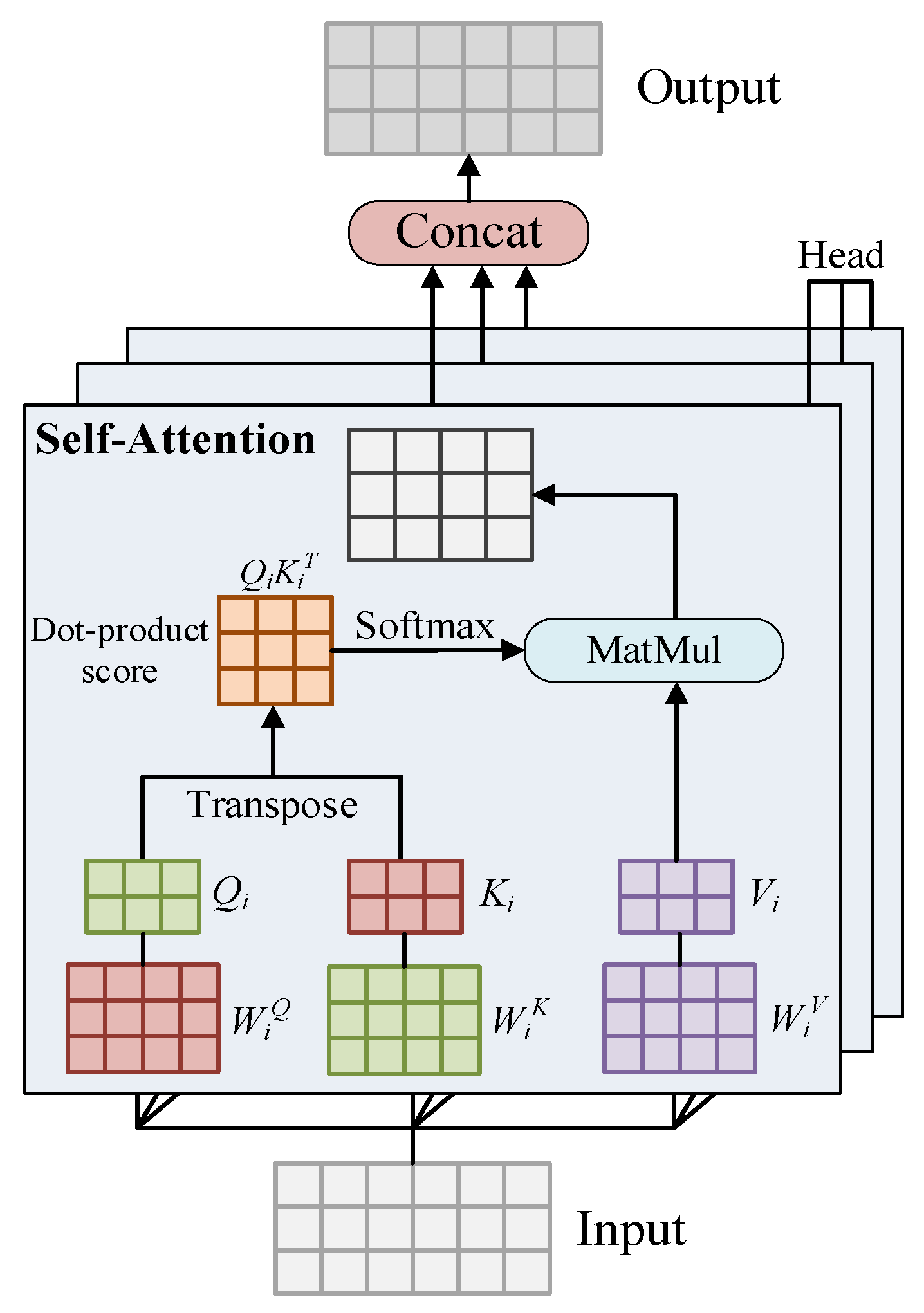
The Transformer is a deep learning model entirely based on self-attention mechanisms, with a basic architecture comprising an encoder and a decoder. The multi-head attention mechanism, as the core component of the encoder, uses multiple sets of independently trainable weights to project input feature vectors into queries, keys, and values, as illustrated in Figure 3. The scalarized attention of the dot-product is then performed in parallel in each attention head, allowing the model to capture diverse patterns of feature interactions across multiple subspaces within the input sequence [54,55,56]. In this study, a lightweight transformer encoder architecture was adopted, consisting of positional embedding, multi-head attention, and feedforward neural network components. To enhance the spatial awareness of the model, multi-frequency sine and cosine functions were used to perform periodic encoding of the latitude and longitude coordinates of all sampling points, thereby generating four-dimensional positional vectors. These vectors were treated as auxiliary features and concatenated with the primary spectral features extracted by CNN, allowing the joint modeling of spatial and spectral information. The computation processes for latitude–longitude-based positional encoding and the multi-head attention mechanism are detailed as follows.
PE i = sin π λ i , cos π λ i , sin π φ i , cos π φ i
Attention Q , K , V = softmax Q K T d k V
head i = Attention Q W i Q , K W i K , V W i V
Multihead Q , K , V = Concat head 1 , head h W O
FFN x = f ReLU W 1 x + b 1 W 2 + b 2
where λi and φi are the normalized longitude and latitude in the range [0,1]; PEi is the spatial positional embedding vector; Q, K, and V are the query, key, and value matrices; headi (i = 1, …, h) is the attention output of the i-th head; Concat is the concatenation operation; WQ, WK, and WV are the projection matrices for each head, and WO is the projection matrix for the multi-head output; x is the input feature vector; fReLU is the nonlinear activation function; and W1, W2, b1, and b2 are the weight matrices and bias terms of the two-layer linear transformation, respectively [57].
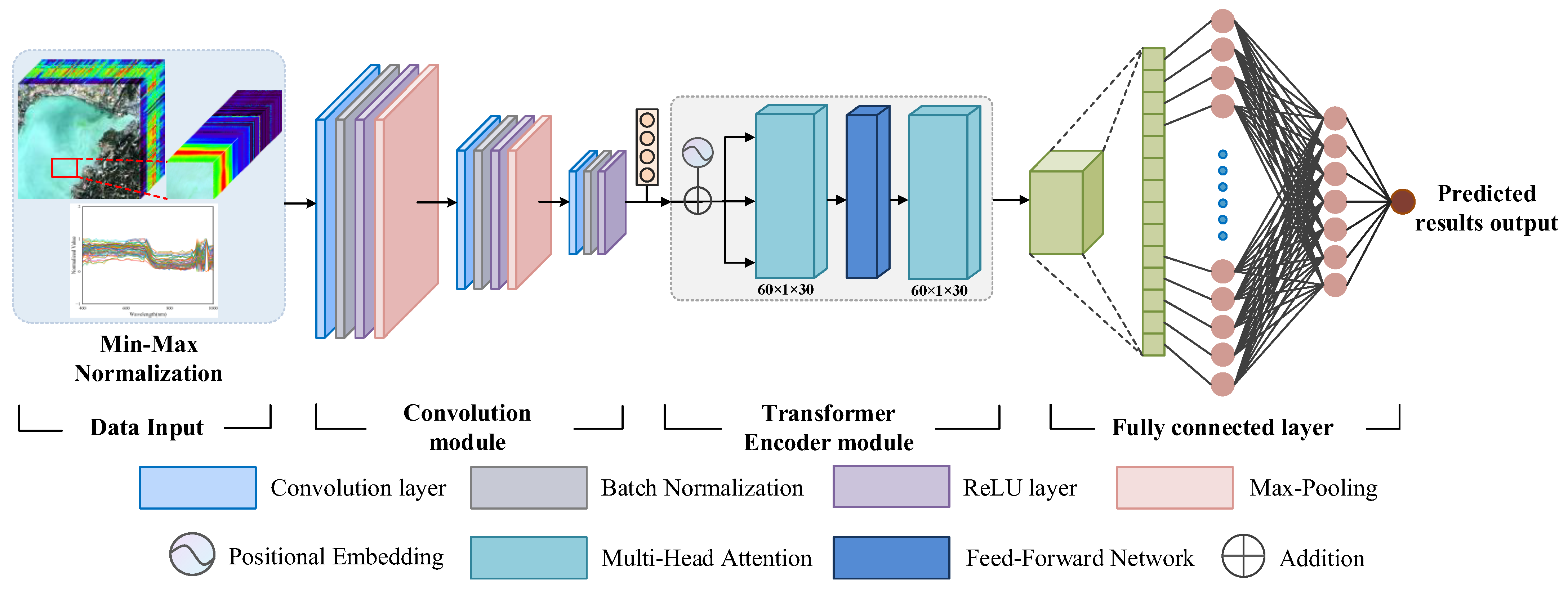
Figure 4 illustrates the architecture of the CMAF-Net model. Initially, CNN is employed as a front-end feature extractor to obtain activated high-dimensional feature vectors from its output. The sequence input layer of the encoder receives fused features formed by concatenating the high-dimensional spectral feature vectors extracted by the CNN with the spatial positional encoding vectors. The positional embedding layer generates a learnable position vector for each feature location in the input spectral sequence with the same dimensionality as the original feature. Each position vector is then added to the corresponding spectral feature, thereby introducing explicit positional information into the sequence representation. Two consecutive multi-head attention layers are used for deep feature extraction, interleaved with a feedforward neural network to further capture the nonlinear structural information within the features refined by the attention mechanism. Finally, a fully connected layer maps the features to a scalar output corresponding to each sample [58].
During training for the CMAF-Net model, dropout layers were introduced to mitigate potential overfitting, and the complexity of the model was further controlled by incorporating learning rate decay and L2 regularization. Regarding hyperparameter settings, the CNN module adopted the same configuration as when the CNN model was run independently. The encoder module was also trained using the Adam optimizer, with a maximum of 100 training epochs and an initial learning rate of 0.01. The number of attention heads was set to 4, with each head having a dimensionality of 32. The dimensionality of the attention key vectors was set to 128, and the maximum positional index of the sequence was set to 256.

2.4. Model Accuracy Evaluation

This study uses the coefficient of determination (R2), root mean square error (RMSE), and residual predictive deviation (RPD) as the primary evaluation metrics, with the mean absolute error (MAE) and symmetric mean absolute percentage error (SMAPE) as supplementary indicators, to comprehensively assess the model performance. R2 measures the fit between the model’s predicted values and the observed data. A value closer to 1 indicates a better fit to the model. RMSE, MAE, and SMAPE quantify prediction errors, with lower values reflecting greater model accuracy. The RPD reflects the reliability of the model’s predictions. It is generally accepted that RPD ≤ 1.4 indicates poor predictive ability; 1.4 < RPD < 2 suggests moderate predictive performance suitable for rough screening; and RPD ≥ 2 implies good predictive capacity, making the model applicable for practical quantitative prediction tasks [59,60].
R 2 = 1 i = 1 n ( y ^ i y i ) 2 i = 1 n ( y i y ¯ ) 2
R M S E = i = 1 n y ^ i y i 2 n
R P D = 1 n 1 i = 1 n y i y ¯ 2 R M S E
M A E = i = 1 n y ^ i y i n
S M A P E = 100 % n i = 1 n y ^ i y i y ^ i + y i / 2
where y ^ i is the predicted value of the i-th sample, yi is the measured value of the i-th sample, y ¯ is the mean of all measured values, and n is the total number of samples.

2.5. Construction of Predictive Models

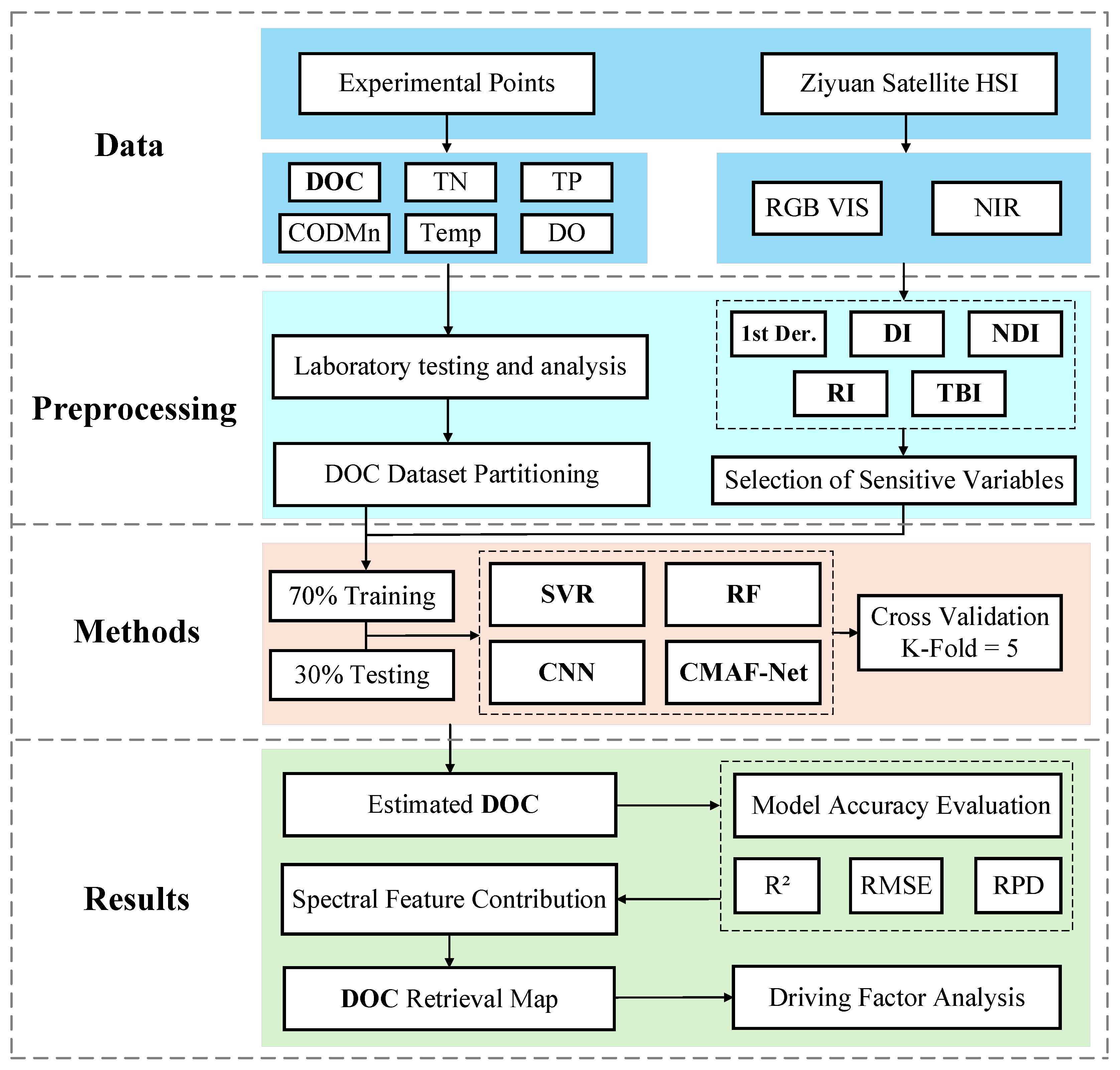
Based on the HSI of the Ziyuan-1 satellite series and the in situ surface water sampling data, four predictive models were applied to estimate DOC concentrations in the lake. The modeling process used the spectral reflectance dataset and corresponding sample data from 60 sampling sites as input. The dataset was randomly divided into training and testing sets in a 7:3 ratio. The training set covered both the high and low value ranges of the testing set, ensuring good generalization ability and applicability of the model. The division of the sample set is presented in Table 3, with 42 samples in the training set and 18 in the testing set. Under different combinations of input variables, the predictive performance of the four models was evaluated using multiple metrics to determine the optimal model for estimating DOC concentration (Figure 5).

3. Results

3.1. Optimal Selection of Characteristic Bands

To enhance the spectral sensitivity of remote sensing features to DOC concentration, the first derivative transformation was used to extract representative bands from the hyperspectral dataset to reduce dimensional redundancy. Within the spectral range of 400–1000 nm, 21 key single-band characteristics were identified based on the peak and trough positions of the first-order spectral derivative curve (as shown in Figure 6a) and the correlation coefficients between the original reflectance bands and DOC concentrations. These selected bands exhibited pronounced spectral variability and were deemed to have potential physical relevance to the DOC distribution. Furthermore, to amplify spectral response differences related to DOC and enhance the model’s ability to capture nonlinear features, this study used several band combination strategies, including the dual-variable difference index (DI), normalized difference index (NDI), ratio indices (RI1, RI2), and the tri-band combination index (TBI) [61,62,63]. The corresponding expressions are presented below.
D I = R λ 1 R λ 2
N D I = R λ 1 R λ 2 / R λ 1 + R λ 2
R I 1 = R λ 1 / R λ 2
R I 2 = R λ 1 / R λ 1 R λ 2
T B I = R λ 1 / R λ 2 R λ 3
where Rλ1, Rλ2, and Rλ3 are the reflectance values at three different spectral bands.
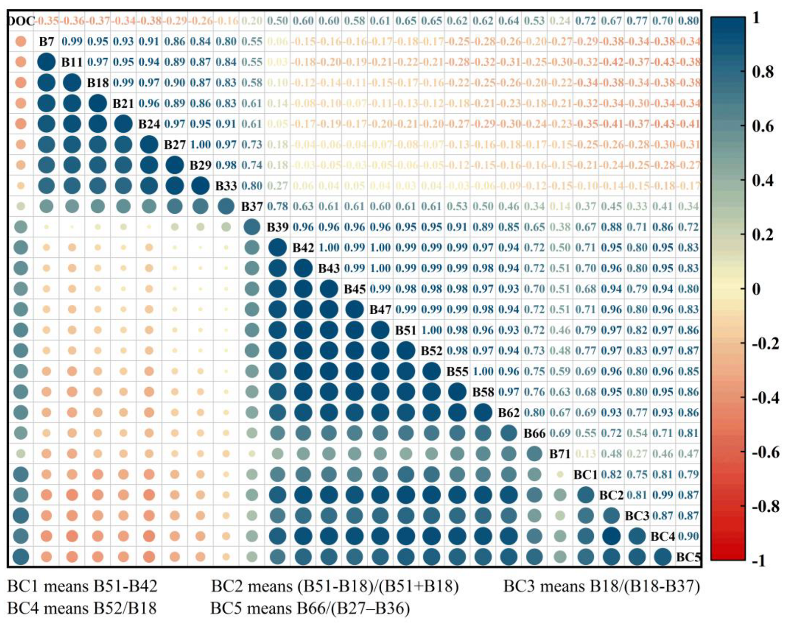
The correlation coefficients of the five spectral indices are shown in Figure 6b–f. As illustrated, the maximum correlation between a single original satellite band and the DOC concentration was 0.65. Following the construction of spectral indices, the correlation between band combinations and DOC increased substantially, reaching values between 0.67 and 0.80. Based on these correlation analyses, the most relevant combination of each index category was selected for subsequent modeling. To preserve the physical interpretability of the spectral data, the selected single-band features were arranged in ascending order of wavelength, forming a spectrally coherent sequence. These were then combined with the selected band combination indices to establish the final set of sensitive spectral variables for modeling. The complete feature set included the following 26 spectral variables: Single-band features: B7, B11, B18, B21, B24, B27, B29, B33, B37, B39, B42, B43, B45, B47, B51, B52, B55, B58, B62, B66, and B71; band combination features: B51−B42, (B51−B18)/(B51+B18), B18/(B18−B37), B52/B18, and B66/(B27−B36). These characteristics were used as input variables for the SVR, RF, CNN, and CMAF-Net models to construct a DOC remote sensing estimation framework. Figure 7 presents the correlation matrix between the final 21 selected single-band characteristics, five-band combination indices, and DOC concentrations. Regions with statistically significant correlations are highlighted, validating the sensitivity and effectiveness of the selected features in relation to measured DOC concentrations.

3.2. DOC Model Analysis

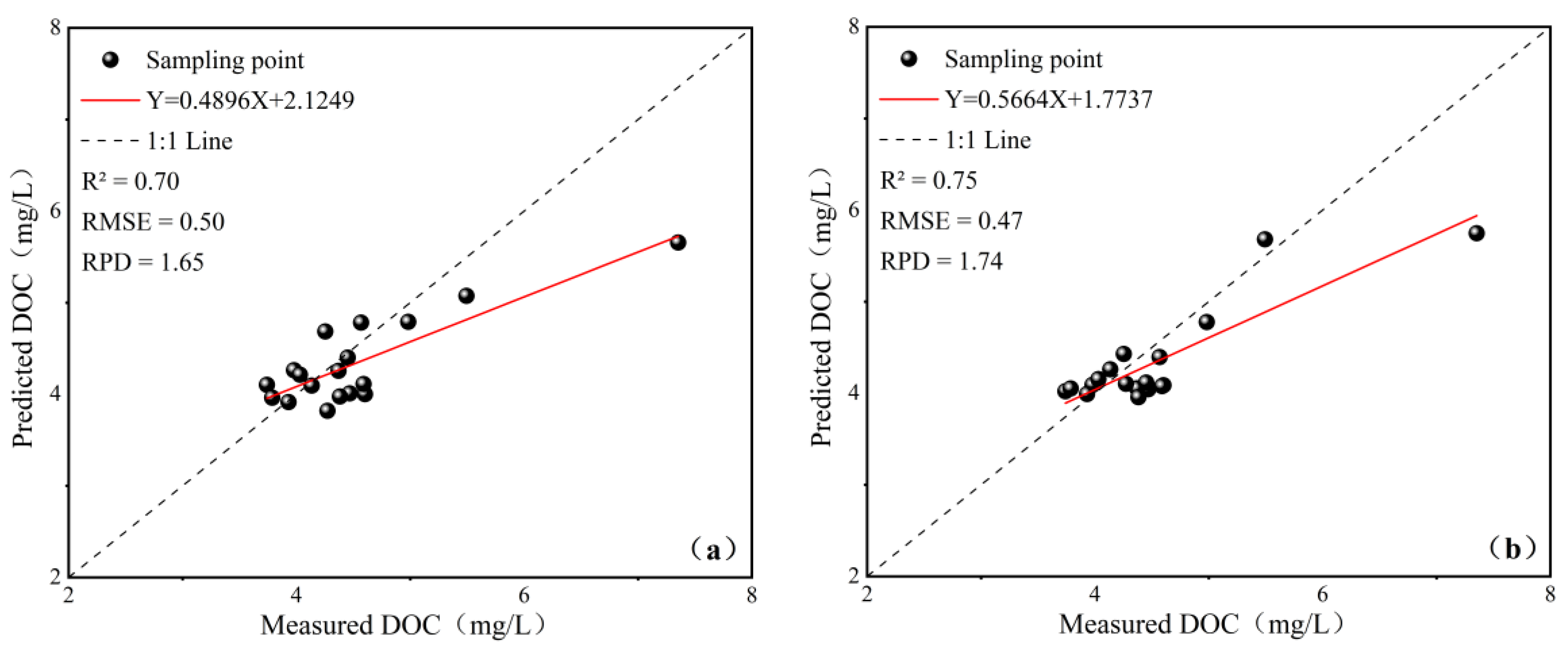
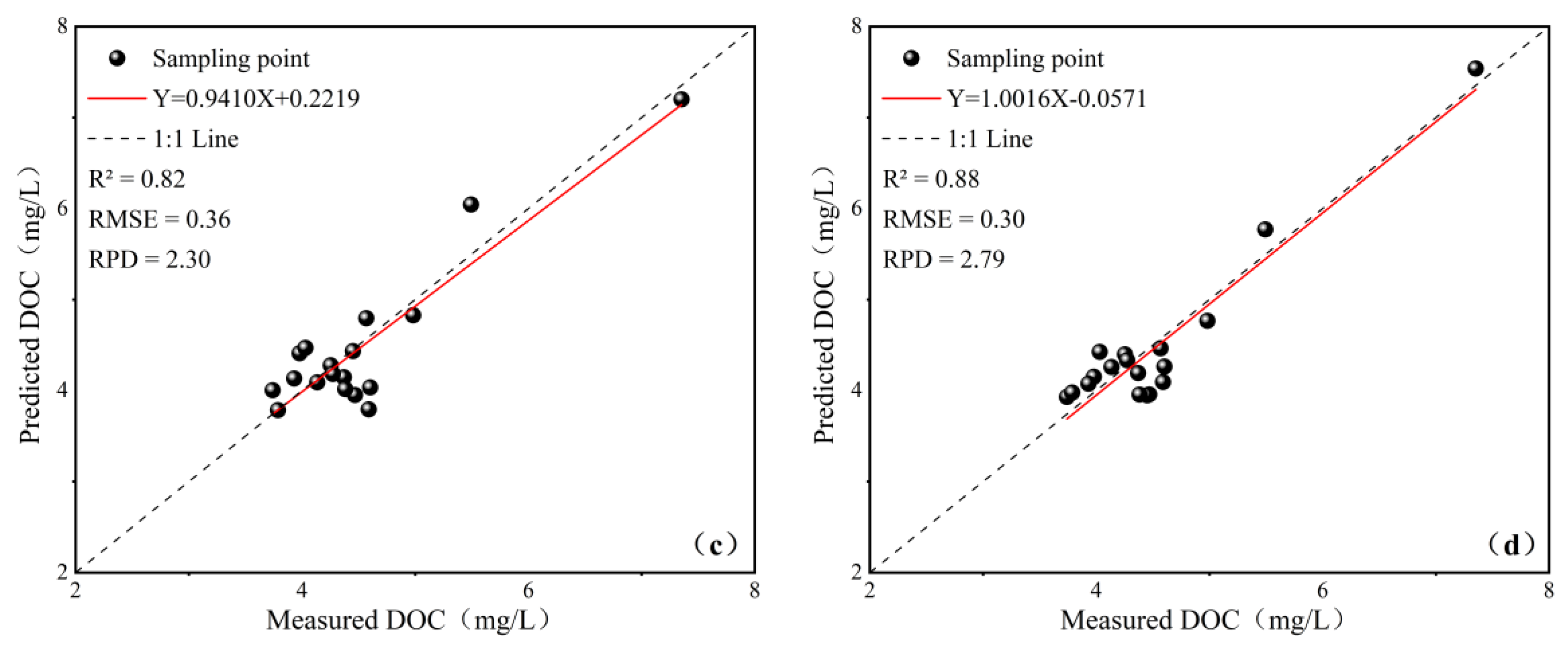
The prediction results of the four models, SVR, RF, CNN, and CMAF-Net are presented in Table 4. As shown in Table 4, the four models achieved RPD values greater than 1.4 in the test set, indicating that each model has a certain level of predictive capacity for the estimation of DOC. Among the models, SVR and RF exhibited relatively weaker overall performance in all evaluation metrics, with limited fit capability and poor agreement between predicted and observed values. A noticeable gap in the R2 values between the training and testing sets indicates a slight overfitting tendency for both models. Compared to SVR, the RF model outperformed for both RMSE and RPD, indicating improved predictive performance. Compared to SVR and RF, the CNN model demonstrated significant improvements in all evaluation metrics, with R2 values of 0.87 and 0.82, RMSE values of 0.32 and 0.36, and RPD values of 3.07 and 2.30, respectively. Finally, as a combined CNN optimization, the CMAF-Net model achieved the best predictive performance, with R2, RMSE, and RPD in the test set reaching 0.88, 0.29, and 2.79, respectively. Compared to CNN in the test set, R2 and RPD increased by 7.32% and 21.3%, while RMSE decreased by 19.4%.
To further analyze the model’s predictive performance on the test set, a scatter regression plot of measured versus predicted values was generated, as shown in Figure 8. The distribution of DOC concentrations between test samples exhibits certain extremes and variability. Among all models, CMAF-Net showed the most compact scatter distribution, with its regression line closely approximating the ideal reference line 1:1. The model maintained reliable prediction accuracy at both high and low concentration levels, indicating strong predictive consistency and robustness across the entire concentration range. Furthermore, it exhibited the highest R2 value, the lowest RMSE, and an RPD well above 2, demonstrating good applicability for DOC quantitative prediction tasks.

3.3. Validation of DOC Prediction Models

To further assess the stability and generalizability of deep learning models in the quantitative prediction of DOC, this study used a five-fold cross-validation strategy to assess the four prediction models (Figure 9). The results are summarized in Table 5. The performance metrics of all models declined compared to the results based on fixed dataset partitioning. However, the CMAF-Net model consistently outperformed the CNN model in all evaluation metrics. Specifically, averaged over the validation folds, the CMAF-Net model achieved a 10% reduction in RMSE compared to CNN, along with improvements of 6.57% and 11.22% in R2 and RPD, respectively. It also showed a smaller standard deviation in R2, along with the lowest MAE and SMAPE values, indicating a lower prediction error and further confirming the good generalizability of the model in the quantitative prediction of DOC.

3.4. Inversion Results and Analysis

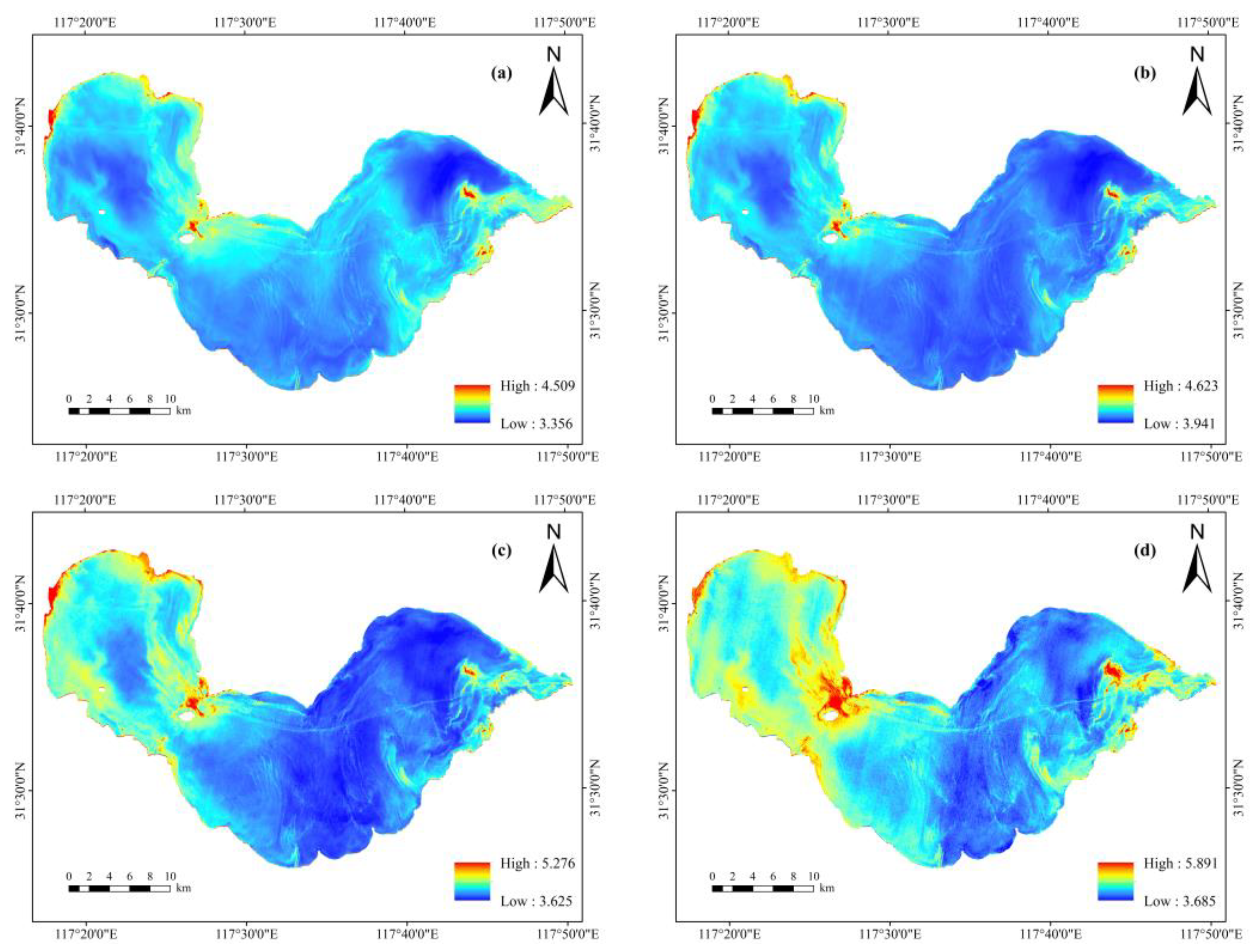
The spatial distribution of the DOC concentrations in the study area was individually retrieved using the four models. As shown in Figure 10, the overall range of DOC concentration retrieved by the SVR, RF, and CNN models in the lake region ranges from 3.356 to 5.276 mg/L. Compared to the two ML models, the CNN model shows notably improved retrieval accuracy in high-concentration areas, and its predictions in low-concentration regions are also closer to the measured values. The CMAF-Net model retrieved DOC concentrations ranging from 3.685 to 5.891 mg/L, showing a wider concentration gradient compared to the CNN model. The mean value retrieved is 4.45 mg/L, which is closest to the mean measured concentration of 4.52 mg/L. Furthermore, the spatial distribution of the DOC retrieved by the CMAF-Net model more closely resembles the original spatial patterns of pollutants of water quality observed in the imagery. It demonstrates better ability to capture localized accumulation and diffusion characteristics of water pollution across different zones, particularly in restoring spatial detail in areas surrounding the lake, river inlets, and island peripheries.
The overall retrieval results indicate that the DOC concentrations in Chaohu Lake during the autumn are higher in the western region, gradually extending toward the central area, while the eastern and central regions exhibit comparatively lower levels. Spatially, the distribution follows a west–high to east–low pattern. The western shoreline of Chaohu Lake is adjacent to the main urban area and several industrial parks. Substantial volumes of domestic wastewater and agricultural runoff enter the western lake region through major inflow rivers such as the Nanfei River, the Shiwuli River, and the Pai River, which can lead to the enrichment of terrestrial organic matter in this area. Additionally, due to the input of organic matter derived from leaf litter during late autumn and early winter, combined with anthropogenic influences, high concentrations of DOC tend to accumulate along the island margins and gradually decrease outward with a diffusion-like spatial pattern.

4. Discussion

4.1. Analysis of Spectral Feature Contributions

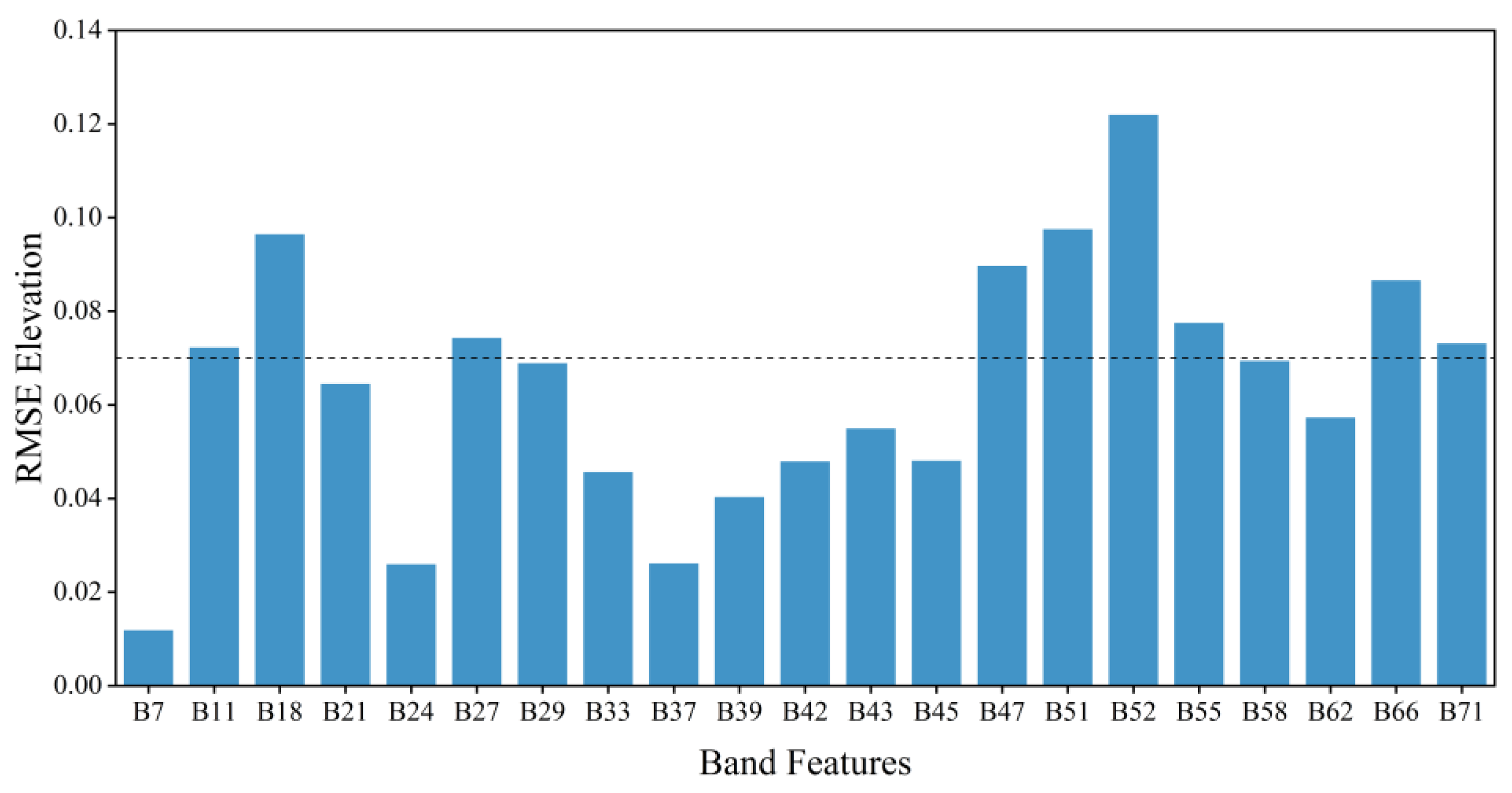
To evaluate the contribution of each input feature to the prediction of the CMAF-Net model, a perturbation-based feature importance analysis was used. Specifically, for each feature, its values in all training samples were replaced with the corresponding mean values, while all other features were kept unchanged. The change in RMSE between the original and perturbed predictions was then calculated and used as an indicator of the contribution of the feature [64,65].
The significance scores for the characteristics are shown in Figure 11. It is evident that the bands associated with larger increases in RMSE are mainly concentrated in the green spectral region near 530 nm and the near-infrared region between 780 and 850 nm. The region around 530 nm corresponds to the reflectance enhancement zone of Chl-a. In eutrophic lakes, increased algal biomass leads to elevated reflectance at this wavelength, and algal activity exhibits strong covariation with DOC concentrations. Therefore, the spectral band around 530 nm may serve as a covariate feature for identifying the variation in DOC [66,67]. Furthermore, the spectral region near 800 nm corresponds to the characteristic reflectance range of SPM and enhanced backscattering from phytoplankton cells. Clustering of high-impact spectral bands in this region is likely to be the result of the combined influence of phytoplankton biomass (proxied by Chl-a) and suspended particles and is also significantly associated with DOC concentrations [68].

4.2. Algorithm Performance

The four models—SVR, RF, CNN, and CMAF-Net—exhibited observable differences in predicting DOC concentrations in lake water. Although the SVR model demonstrates stable performance in small-sample modeling, it has limited capability in capturing nonlinear relationships among high-dimensional features. As an ensemble learning method, the RF model possesses certain nonlinear fitting capabilities and a built-in mechanism for assessing the importance of features. However, due to its tree-based structure, it treats each spectral band as an independent input variable, which often neglects potential spectral interactions between bands. While the multi-layer structure of the CNN model demonstrates advantages in handling complex nonlinear problems under high feature dimensionality, its weight-sharing mechanism applies the same set of convolutional kernel parameters across the entire spectral sequence. Although this improves local perception, it also enforces uniform weighting for all features, thus limiting the ability of the model to perform global modeling with differentiated spectral band weights [69]. To enhance the predictive performance of the model, multi-head attention mechanisms were introduced, allowing the model to autonomously focus on key spectral regions that are more sensitive to DOC concentration within the hyperspectral band sequence, providing adaptive weighted enhancement for feature learning [70]. This finding is consistent with the results of Ahmad et al. [71]. and Shanthini et al. [72], which highlight the advantage of integrating attention mechanisms into CNN-based hyperspectral modeling frameworks.
Although baseline CNNs perform well in DOC prediction, their convolutional kernel sizes and weight-sharing mechanisms limit the full exploration of spectral representations and entail strong dependence on data scale and computational resources [73]. CMAF-Net, by adaptively weighting to suppress interference from redundant spectral bands and focus on key spectral segments, retains the CNN’s advantage in local spectral feature representation while achieving a more compact nonlinear mapping with fewer parameters. Despite introducing an attention module, its overall computational overhead and training time are comparable to those of a plain CNN, enabling efficient feature extraction and spectral-sequence modeling and avoiding high noise and excessive details during training, thereby mitigating the risk of overfitting under small-sample conditions [74]. Meanwhile, in this study, the model maintained good predictive accuracy and stability even under skewed DOC concentration distributions with extremely high values.

4.3. Analysis of Driving Factors

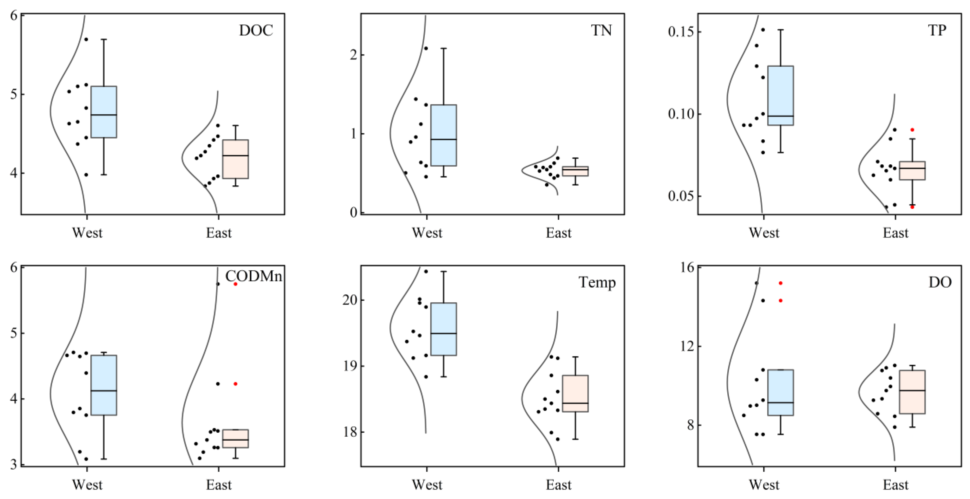
The spatial heterogeneity of DOC in the lake may be related to the influence of environmental factors in the water. To explore the driving factors affecting DOC, this study used data from the second sampling campaign. The sampling sites were classified into eastern and western lake regions, and the distribution patterns of DOC, TN, TP, DO, CODMn, and water temperature were illustrated under relatively consistent seasonal conditions, as shown in Figure 12.
As shown in the boxplots, the western part of the lake not only exhibits higher median values but also displays broader interquartile ranges, indicating greater variability in environmental factors of water. Overall, DO levels in the western half of the lake fluctuate significantly. The concentrations of TN, TP, CODMn, and water temperature are higher in the western region than in the eastern region, with particularly pronounced differences observed for TN, TP, and water temperature. The western part of Chaohu Lake has a relatively low-lying topography with shallow waters near the shore. Combined with the urban heat island effect and high-intensity inputs of nutrients such as nitrogen and phosphorus, this results in overall higher water temperatures compared to the eastern part of the lake, making it prone to the formation of localized stable zones with weak exchange efficiency [75]. The spatial heterogeneity of water quality parameters shaped by the synergistic effects of nutrient flux, hydrodynamic structure, and thermal background has also been widely observed and validated in typical eutrophic water bodies such as Taihu Lake, Dongting Lake, and the Yangtze River Estuary [76,77,78].
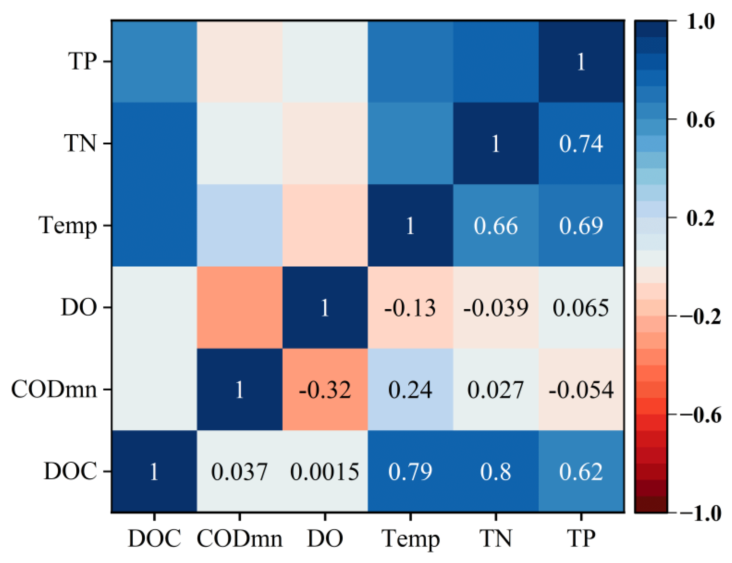
To further investigate the relationship between DOC and the five parameters of water quality, a Pearson correlation analysis was performed to assess pairwise associations among the variables, as shown in Figure 13.
The results showed that DOC was significantly positively correlated with TN (r = 0.80) and TP (r = 0.62). This suggests that the increase in DOC may be attributed to the release of large amounts of organic matter derived from algae after algal senescence in eutrophic lakes dominated by endogenous nitrogen and phosphorus inputs [79,80]. Corman et al. also suggested that nutrient loading associated with dissolved organic matter may lead to significant increases in N and P within lake systems [81], implying that there is a reciprocal driving influence between DOC and N and P. Meanwhile, the significant correlation between DOC and water temperature (r = 0.79) indicated that water temperature may be an important factor in promoting extended periods of the growth of aquatic plants and improving microbial decomposition and release, thus indirectly affecting DOC concentration [82,83]. On the contrary, DO and CODMn showed weaker correlations with DOC, suggesting that they may not serve as major regulatory factors in the biogeochemical framework of this lake system.

4.4. Limitations and Future Research

The input features of current prediction algorithms are mainly limited to hyperspectral remote sensing bands and their combination indices, and the feature sources are relatively single. For inland water bodies with complex optical properties, the source mechanisms of DOC are diverse and coupled with covariant factors such as Chl-a, SPM, and CDOM, which are prone to cause inter-spectral interference and result in aliasing of reflected signals [84]. Based on the enhancement of key spectral features through the adaptive weight allocation of CMAF-Net, in the future, multi-source auxiliary variables, such as water quality parameters and environmental indicators that are significantly covariant with DOC, will be collected and introduced to expand the input dimension. The characterization of the nonlinear relationship between DOC and spectral features will be further enhanced through multi-factor collaborative modeling, thereby strengthening the decoupling of complex hyperspectral signals and improving the generalization performance of the model.

5. Conclusions

Using Chaohu Lake as a case study, this study employed HSI from the Chinese Ziyuan-1 series to propose CMAF-Net, a hybrid deep learning model for estimating lake dissolved DOC concentrations. Based on model-based retrievals, the spatial distribution of DOC and its driving factors across the lake were further examined. The main conclusions are as follows.
(1)
The SVR, RF, and CNN models exhibited a certain level of predictive capacity for DOC in inland lakes. Among them, the CNN model performed best, achieving an R2 of 0.82, an RMSE of 0.36 mg/L, and an RPD of 2.30. After constructing CMAF-Net by combining the lightweight Transformer encoder with CNN, R2 reached 0.88, RMSE was 0.29 mg/L, and RPD was 2.79, within the range of high performance. Compared to CNN alone, R2 and RPD increased by 7.32% and 21.3%, respectively, and RMSE decreased by 19.4%, indicating that the introduction of the attention mechanism significantly enhanced the ability of the CNN model to identify key spectral features.
(2)
Satellite-based retrieval results show that the DOC concentration in Chaohu Lake ranges from 3.685 to 5.891 mg/L, with an average concentration of 4.45 mg/L. Higher concentrations of DOC are observed in the western part of the lake, around the islands, and near the river inflow zones, while lower concentrations appear in the central and eastern regions. Overall, the spatial distribution of the DOC exhibited a clear west–high to east–low pattern. This spatial heterogeneity reflects the combined effects of regional nutrient inputs, hydrodynamic conditions, and anthropogenic activities.
(3)
Five water environmental variables generally showed higher concentrations in the western half of Chaohu Lake. Among them, nitrogen, phosphorus, and water temperature were strongly positively correlated with DOC concentrations, suggesting that they are the main drivers of the spatial patterns of DOC in Chaohu Lake.
In summary, the CMAF-Net model combined with hyperspectral remote sensing provides a feasible deep learning modeling framework for the high-precision retrieval of DOC in inland lake waters. In the future, CMAF-Net can be further extended to multi-temporal and multi-type inland waters by incorporating time series remote sensing data to improve the timeliness and universality of the model, which will support the development of more stable and adaptive environmental monitoring techniques, contributing to the scientific management and ecological protection of watershed resources.

Author Contributions

Conceptualization and writing original draft preparation: Q.G. and W.L.; methodology: Q.W. and L.H.; supervision: Y.S. and J.D.; data curation: Q.G. and Z.D.; writing—review and editing supported by Q.G. and J.L.; funding acquisition: B.P. All authors have read and agreed to the published version of the manuscript.

Funding

The author gratefully acknowledges the financial support from the National Natural Science Foundation of China (42277075), Key Science and Technology Projects under the Science and Technology Innovation Platform (202305a12020039), the Anhui Natural Science Research Foundation (2208085US14), the Anhui Provincial Science and Technology Plan Project for Housing and Urban-Rural Construction (2024-YF055), and the Natural Science Foundation of Colleges and Universities in Anhui Province (2023AH050187).

Institutional Review Board Statement

Not applicable.

Informed Consent Statement

Not applicable.

Data Availability Statement

The original contributions presented in the study are included in the article; further inquiries can be directed to the corresponding author.

Conflicts of Interest

The authors declare no conflicts of interest.

References

  1. Xiao, Q.; Xu, X.; Qi, T.; Luo, J.; Lee, X.; Duan, H. Lakes Shifted from a Carbon Dioxide Source to a Sink over Past Two Decades in China. Sci. Bull. 2024, 69, 1857–1861. [Google Scholar] [CrossRef]
  2. Wang, S.; Gao, Y.; Jia, J.; Lu, Y.; Wang, J.; Ha, X.; Li, Z.; Sun, K. Determining Whether Hydrological Processes Drive Carbon Source and Sink Conversion Shifts in a Large Floodplain-Lake System in China. Water Res. 2022, 224, 119105. [Google Scholar] [CrossRef]
  3. Zhou, L.; Zhou, Y.; Zhang, Y.; Jeppesen, E.; Weyhenmeyer, G.A. Rainstorm-Induced Organic Matter Pulses: A Key Driver of Carbon Emissions from Inland Waters. Innov. 2025, 6, 100746. [Google Scholar] [CrossRef]
  4. Paíz, R.; Pierson, D.C.; Lindqvist, K.; Naden, P.S.; De Eyto, E.; Dillane, M.; McCarthy, V.; Linnane, S.; Jennings, E. Accounting for Model Parameter Uncertainty Provides More Robust Projections of Dissolved Organic Carbon Dynamics to Aid Drinking Water Management. Water Res. 2025, 276, 123238. [Google Scholar] [CrossRef]
  5. Liu, S.; Hou, J.; Suo, C.; Chen, J.; Liu, X.; Fu, R.; Wu, F. Molecular-Level Composition of Dissolved Organic Matter in Distinct Trophic States in Chinese Lakes: Implications for Eutrophic Lake Management and the Global Carbon Cycle. Water Res. 2022, 217, 118438. [Google Scholar] [CrossRef] [PubMed]
  6. Guo, Y.; Peng, H.; Wang, Q.; Wang, J.; Wu, Z.; Shao, B.; Xing, G.; Huang, Z.; Zhao, F.; Cui, H.; et al. Unveiling the Global Dynamics of Dissolved Organic Carbon in Aquatic Ecosystems: Climatic and Anthropogenic Impact, and Future Predictions. Sci. Total Environ. 2025, 958, 178109. [Google Scholar] [CrossRef] [PubMed]
  7. Liu, S.; He, Z.; Tang, Z.; Liu, L.; Hou, J.; Li, T.; Zhang, Y.; Shi, Q.; Giesy, J.P.; Wu, F. Linking the Molecular Composition of Autochthonous Dissolved Organic Matter to Source Identification for Freshwater Lake Ecosystems by Combination of Optical Spectroscopy and FT-ICR-MS Analysis. Sci. Total Environ. 2020, 703, 134764. [Google Scholar] [CrossRef] [PubMed]
  8. Pilla, R.M.; Couture, R. Attenuation of Photosynthetically Active Radiation and Ultraviolet Radiation in Response to Changing Dissolved Organic Carbon in Browning Lakes: Modeling and Parametrization. Limnol. Oceanogr. 2021, 66, 2278–2289. [Google Scholar] [CrossRef]
  9. Shen, C.; Qian, M.; Song, Y.; Chen, B.; Yang, J. Surface pCO2 and Air-Water CO2 Fluxes Dominated by Submerged Aquatic Vegetation: Implications for Carbon Flux in Shallow Lakes. J. Environ. Manag. 2024, 370, 122839. [Google Scholar] [CrossRef]
  10. Sun, Y.; Wang, D.; Li, L.; Ning, R.; Yu, S.; Gao, N. Application of Remote Sensing Technology in Water Quality Monitoring: From Traditional Approaches to Artificial Intelligence. Water Res. 2024, 267, 122546. [Google Scholar] [CrossRef]
  11. Zhao, Z.; Shi, K.; Zhang, Y. Remote Sensing Estimation of Dissolved Organic Carbon Concentrations in Chinese Lakes Based on Landsat Images. J. Hydrol. 2024, 638, 131466. [Google Scholar] [CrossRef]
  12. Bonelli, A.G.; Loisel, H.; Jorge, D.S.F.; Mangin, A.; d’Andon, O.F.; Vantrepotte, V. A New Method to Estimate the Dissolved Organic Carbon Concentration from Remote Sensing in the Global Open Ocean. Remote Sens. Environ. 2022, 281, 113227. [Google Scholar] [CrossRef]
  13. Niu, C.; Tan, K.; Wang, X.; Pan, C. Mapping Nutrient Pollution in Inland Water Bodies Using Multi-Platform Hyperspectral Imagery and Deep Regression Network. J. Hazard. Mater. 2025, 488, 137314. [Google Scholar] [CrossRef] [PubMed]
  14. Bai, X.; Wang, J.; Chen, R.; Kang, Y.; Ding, Y.; Lv, Z.; Ding, D.; Feng, H. Research Progress of Inland River Water Quality Monitoring Technology Based on Unmanned Aerial Vehicle Hyperspectral Imaging Technology. Environ. Res. 2024, 257, 119254. [Google Scholar] [CrossRef]
  15. El Alem, A.; Chokmani, K.; Venkatesan, A.; Lhissou, R.; Martins, S.; Campbell, P.; Cardille, J.; McGeer, J.; Smith, S. Modeling Dissolved Organic Carbon in Inland Waters Using an Unmanned Aerial Vehicles-Borne Hyperspectral Camera. Sci. Total Environ. 2024, 954, 176258. [Google Scholar] [CrossRef] [PubMed]
  16. Wei, L.; Wang, Z.; Huang, C.; Zhang, Y.; Wang, Z.; Xia, H.; Cao, L. Transparency Estimation of Narrow Rivers by UAV-Borne Hyperspectral Remote Sensing Imagery. IEEE Access 2020, 8, 168137–168153. [Google Scholar] [CrossRef]
  17. Dev, P.J.; Sukenik, A.; Mishra, D.R.; Ostrovsky, I. Cyanobacterial Pigment Concentrations in Inland Waters: Novel Semi-Analytical Algorithms for Multi- and Hyperspectral Remote Sensing Data. Sci. Total Environ. 2022, 805, 150423. [Google Scholar] [CrossRef]
  18. Li, J.; Zheng, Z.; Li, Y.; Lyu, H.; Ren, J.; Cai, X.; Du, C.; Chen, N.; Liu, G.; Lei, S.; et al. A Hybrid Algorithm for Estimating Total Nitrogen from a Large Eutrophic Plateau Lake Using Orbita Hyperspectral (OHS) Satellite Imagery. Int. J. Appl. Earth Obs. Geoinf. 2024, 131, 103971. [Google Scholar] [CrossRef]
  19. Mobley, C.; Stramski, D.; Bissett, P.; Boss, E. Optical Modeling of Ocean Waters: Is the Case 1-Case 2 Classification Still Useful? Oceanography 2004, 17, 60–67. [Google Scholar] [CrossRef]
  20. O’Shea, R.E.; Pahlevan, N.; Smith, B.; Boss, E.; Gurlin, D.; Alikas, K.; Kangro, K.; Kudela, R.M.; Vaičiūtė, D. A Hyperspectral Inversion Framework for Estimating Absorbing Inherent Optical Properties and Biogeochemical Parameters in Inland and Coastal Waters. Remote Sens. Environ. 2023, 295, 113706. [Google Scholar] [CrossRef]
  21. Lee, C.-M.; Kuo, C.-Y.; Yang, C.-H.; Kao, H.-C.; Tseng, K.-H.; Lan, W.-H. Assessment of Hydrological Changes in Inland Water Body Using Satellite Altimetry and Landsat Imagery: A Case Study on Tsengwen Reservoir. J. Hydrol. Reg. Stud. 2022, 44, 101227. [Google Scholar] [CrossRef]
  22. Wu, Y.; Knudby, A.; Pahlevan, N.; Lapen, D.; Zeng, C. Sensor-Generic Adjacency-Effect Correction for Remote Sensing of Coastal and Inland Waters. Remote Sens. Environ. 2024, 315, 114433. [Google Scholar] [CrossRef]
  23. Tao, H.; Song, K.; Wen, Z.; Liu, G.; Shang, Y.; Fang, C.; Wang, Q. Remote Sensing of Total Suspended Matter of Inland Waters: Past, Current Status, and Future Directions. Ecol. Inform. 2025, 86, 103062. [Google Scholar] [CrossRef]
  24. Deng, Y.; Zhang, Y.; Pan, D.; Yang, S.X.; Gharabaghi, B. Review of Recent Advances in Remote Sensing and Machine Learning Methods for Lake Water Quality Management. Remote Sens. 2024, 16, 4196. [Google Scholar] [CrossRef]
  25. Huang, H.; Zhang, J. Prediction of Chlorophyll a and Risk Assessment of Water Blooms in Poyang Lake Based on a Machine Learning Method. Environ. Pollut. 2024, 347, 123501. [Google Scholar] [CrossRef] [PubMed]
  26. Ozbayram, O.; Olivier, A.; Graham-Brady, L. Heteroscedastic Gaussian Process Regression for Material Structure–Property Relationship Modeling. Comput. Methods Appl. Mech. Eng. 2024, 431, 117326. [Google Scholar] [CrossRef]
  27. Codden, C.J.; Snauffer, A.M.; Mueller, A.V.; Edwards, C.R.; Thompson, M.; Tait, Z.; Stubbins, A. Predicting Dissolved Organic Carbon Concentration in a Dynamic Salt Marsh Creek via Machine Learning. Limnol. Ocean. Methods 2021, 19, 81–95. [Google Scholar] [CrossRef]
  28. Harkort, L.; Duan, Z. Estimation of Dissolved Organic Carbon from Inland Waters at a Large Scale Using Satellite Data and Machine Learning Methods. Water Res. 2023, 229, 119478. [Google Scholar] [CrossRef]
  29. Reichstein, M.; Camps-Valls, G.; Stevens, B.; Jung, M.; Denzler, J.; Carvalhais, N. Prabhat Deep Learning and Process Understanding for Data-Driven Earth System Science. Nature 2019, 566, 195–204. [Google Scholar] [CrossRef]
  30. Rubin, H.J.; Lutz, D.A.; Steele, B.G.; Cottingham, K.L.; Weathers, K.C.; Ducey, M.J.; Palace, M.; Johnson, K.M.; Chipman, J.W. Remote Sensing of Lake Water Clarity: Performance and Transferability of Both Historical Algorithms and Machine Learning. Remote Sens. 2021, 13, 1434. [Google Scholar] [CrossRef]
  31. Ali, A.; Zhou, G.; Pablo Antezana Lopez, F.; Xu, C.; Jing, G.; Tan, Y. Deep Learning for Water Quality Multivariate Assessment in Inland Water across China. Int. J. Appl. Earth Obs. Geoinf. 2024, 133, 104078. [Google Scholar] [CrossRef]
  32. Kandasamy, L.; Mahendran, A.; Sangaraju, S.H.V.; Mathur, P.; Faldu, S.V.; Mazzara, M. Enhanced Remote Sensing and Deep Learning Aided Water Quality Detection in the Ganges River, India Supporting Monitoring of Aquatic Environments. Results Eng. 2025, 25, 103604. [Google Scholar] [CrossRef]
  33. Pyo, J.; Park, L.J.; Pachepsky, Y.; Baek, S.-S.; Kim, K.; Cho, K.H. Using Convolutional Neural Network for Predicting Cyanobacteria Concentrations in River Water. Water Res. 2020, 186, 116349. [Google Scholar] [CrossRef] [PubMed]
  34. Gandhimathi, G.; Chellaswamy, C.; Thiruvalar Selvan, P. Comprehensive River Water Quality Monitoring Using Convolutional Neural Networks and Gated Recurrent Units: A Case Study along the Vaigai River. J. Environ. Manag. 2024, 365, 121567. [Google Scholar] [CrossRef] [PubMed]
  35. Fichot, C.G.; Tzortziou, M.; Mannino, A. Remote Sensing of Dissolved Organic Carbon (DOC) Stocks, Fluxes and Transformations along the Land-Ocean Aquatic Continuum: Advances, Challenges, and Opportunities. Earth-Sci. Rev. 2023, 242, 104446. [Google Scholar] [CrossRef]
  36. Aleissaee, A.A.; Kumar, A.; Anwer, R.M.; Khan, S.; Cholakkal, H.; Xia, G.-S.; Khan, F.S. Transformers in Remote Sensing: A Survey. Remote Sens. 2023, 15, 1860. [Google Scholar] [CrossRef]
  37. Dosovitskiy, A.; Beyer, L.; Kolesnikov, A.; Weissenborn, D.; Zhai, X.; Unterthiner, T.; Dehghani, M.; Minderer, M.; Heigold, G.; Gelly, S.; et al. An Image Is Worth 16 × 16 Words: Transformers for Image Recognition at Scale 2021. arXiv 2020, arXiv:2010.11929. [Google Scholar]
  38. Zhang, W.; Hu, M.; Hou, S.; Shang, R.; Feng, J.; Xu, S. Group-Spectral Superposition and Position Self-Attention Transformer for Hyperspectral Image Classification. Expert Syst. Appl. 2025, 265, 125846. [Google Scholar] [CrossRef]
  39. Shang, R.; Yang, J.; Feng, J.; Li, Y.; Xu, S. Hyperspectral Image Classification Based on ConvGRU and Spectral–Spatial Joint Attention. Appl. Soft Comput. 2025, 174, 112949. [Google Scholar] [CrossRef]
  40. Abidi, S.; Sellami, A. Attention-Driven Multi-Feature Fusion for Hyperspectral Image Classification via Multi-Criteria Optimization and Multi-View Convolutional Neural Networks. Eng. Appl. Artif. Intell. 2024, 138, 109434. [Google Scholar] [CrossRef]
  41. Zhang, Y.; Fu, H.; Yang, X.; Liu, Z. Anthropogenically Driven Changes to Organic Matter Input in Sediments of Lake Chaohu, Eastern China, over the Past 166 Years. CATENA 2023, 231, 107285. [Google Scholar] [CrossRef]
  42. Zhou, T.; Li, Y.; Jiang, B.; Alatalo, J.M.; Li, C.; Ni, C. Tracking Spatio-Temporal Dynamics of Harmful Algal Blooms Using Long-Term MODIS Observations of Chaohu Lake in China from 2000 to 2021. Ecol. Indic. 2023, 146, 109842. [Google Scholar] [CrossRef]
  43. Guo, X.; Liu, H.; Zhong, P.; Hu, Z.; Cao, Z.; Shen, M.; Tan, Z.; Liu, W.; Liu, C.; Li, D.; et al. Remote Retrieval of Dissolved Organic Carbon in Rivers Using a Hyperspectral Drone System. Int. J. Digit. Earth 2024, 17, 2358863. [Google Scholar] [CrossRef]
  44. Tian, X.; Liu, M.; Li, Z.; Gao, X.; Yang, R.; Ni, M.; Xu, Y.J.; Wang, Y.; Ye, C.; Yuan, D.; et al. Eutrophication Constrains Driving Forces of Dissolved Organic Carbon Biodegradation in Metropolitan Lake Systems. Sci. Total Environ. 2024, 953, 176177. [Google Scholar] [CrossRef]
  45. Cai, G.; Zhang, J.; Li, W.; Zhang, J.; Liu, Y.; Xi, S.; Li, G.; Li, H.; Chen, X.; Song, F.; et al. Spatiotemporal Variation and Influencing Factors of Phosphorus in Asia’s Longest River Based on Receptor Model and Machine Learning. Ecol. Indic. 2025, 171, 113217. [Google Scholar] [CrossRef]
  46. GB/T 11892-1989; Water Quality—Determination of Permanganate Index. Standards Press of China: Beijing, China, 1989.
  47. Zhang, J.; Wang, M.; Yang, K.; Zhao, H. Inversion Monitoring of Heavy Metal Pollution in Corn Crops Based on ZY-1 02D Hyperspectral Imaging. Microchem. J. 2025, 208, 112305. [Google Scholar] [CrossRef]
  48. Wu, Z.; Liu, Y.; Fang, S.; Shen, W.; Li, X.; Mao, Z.; Wu, S. Integration of Geographic Features and Bathymetric Inversion in the Yangtze River’s Nantong Channel Using Gradient Boosting Machine Algorithm with ZY-1E Satellite and Multibeam Data. Geomatica 2024, 76, 100027. [Google Scholar] [CrossRef]
  49. Subi, X.; Eziz, M.; Zhong, Q.; Li, X. Estimating the Chromium Concentration of Farmland Soils in an Arid Zone from Hyperspectral Reflectance by Using Partial Least Squares Regression Methods. Ecol. Indic. 2024, 161, 111987. [Google Scholar] [CrossRef]
  50. Song, C.; Xu, Y.; Fang, C.; Zhang, C.; Xin, Z.; Liu, Z. SVR Model and OLCI Images Reveal a Declining Trend in Phycocyanin Levels in Typical Lakes across Northeast China. Ecol. Inform. 2025, 85, 102965. [Google Scholar] [CrossRef]
  51. Scornet, E.; Biau, G.; Vert, J.-P. Consistency of Random Forests. Ann. Statist. 2015, 43, 1716–1741. [Google Scholar] [CrossRef]
  52. Wang, P.; Liu, Y.; Li, Y.; Tang, X.; Ren, Q. Power Prediction for Salinity-Gradient Osmotic Energy Conversion Based on Multiscale and Multidimensional Convolutional Neural Network. Energy 2024, 313, 133729. [Google Scholar] [CrossRef]
  53. Soylu, E.; Gül, S.; Koca, K.A.; Türkoğlu, M.; Terzi, M.; Şengür, A. Speech Signal-Based Accurate Neurological Disorders Detection Using Convolutional Neural Network and Recurrent Neural Network Based Deep Network. Eng. Appl. Artif. Intell. 2025, 149, 110558. [Google Scholar] [CrossRef]
  54. Zhang, Y.; Li, G.; Zhang, X.-P.; He, Y. A Deep Learning Model Based on Transformer Structure for Radar Tracking of Maneuvering Targets. Inf. Fusion 2024, 103, 102120. [Google Scholar] [CrossRef]
  55. Wang, W.; Sun, Q.; Zhang, L.; Ren, P.; Wang, J.; Ren, G.; Liu, B. A Spatial–Spectral Fusion Convolutional Transformer Network with Contextual Multi-Head Self-Attention for Hyperspectral Image Classification. Neural Netw. 2025, 187, 107350. [Google Scholar] [CrossRef] [PubMed]
  56. Dong, L.; Wang, H.; Lou, J. A Temporal Prediction Model for Ship Maneuvering Motion Based on Multi-Head Attention Mechanism. Ocean. Eng. 2024, 309, 118464. [Google Scholar] [CrossRef]
  57. Vaswani, A.; Shazeer, N.; Parmar, N.; Uszkoreit, J.; Jones, L.; Gomez, A.N.; Kaiser, Ł.; Polosukhin, I. Attention Is All You Need. arXiv 2017, arXiv:1706.03762. [Google Scholar]
  58. Gu, X.; See, K.W.; Li, P.; Shan, K.; Wang, Y.; Zhao, L.; Lim, K.C.; Zhang, N. A Novel State-of-Health Estimation for the Lithium-Ion Battery Using a Convolutional Neural Network and Transformer Model. Energy 2023, 262, 125501. [Google Scholar] [CrossRef]
  59. Lei, H.; Bao, N.; Yu, M.; Cao, Y. Estimating and Mapping Tailings Properties of the Largest Iron Cluster in China for Resource Potential and Reuse: A New Perspective from Interpretable CNN Model and Proposed Spectral Index Based on Hyperspectral Satellite Imagery. Int. J. Appl. Earth Obs. Geoinf. 2025, 139, 104512. [Google Scholar] [CrossRef]
  60. Yue, X.; Bai, Y.; Yu, Q.; Ding, L.; Song, W.; Liu, W.; Ren, H.; Song, Q. Novel Hybrid Data-Driven Modeling Based on Feature Space Reconstruction and Multihead Self-Attention Gated Recurrent Unit: Applied to PM2.5 Concentrations Prediction. Sci. Rep. 2025, 15, 17087. [Google Scholar] [CrossRef]
  61. Cao, X.; Zhang, J.; Meng, H.; Lai, Y.; Xu, M. Remote Sensing Inversion of Water Quality Parameters in the Yellow River Delta. Ecol. Indic. 2023, 155, 110914. [Google Scholar] [CrossRef]
  62. Gao, C.; Yan, X.; Qiao, X.; Wei, K.; Zhang, X.; Yang, S.; Wang, C.; Yang, W.; Feng, M.; Xiao, L.; et al. Multivariate Prediction of Soil Aggregate-Associated Organic Carbon by Simulating Satellite Sensor Bands. Comput. Electron. Agric. 2023, 209, 107859. [Google Scholar] [CrossRef]
  63. Zhao, C.; Pan, Y.; Ren, S.; Gao, Y.; Wu, H.; Ma, G. Accurate Vegetation Destruction Detection Using Remote Sensing Imagery Based on the Three-Band Difference Vegetation Index (TBDVI) and Dual-Temporal Detection Method. Int. J. Appl. Earth Obs. Geoinf. 2024, 127, 103669. [Google Scholar] [CrossRef]
  64. Cottin, A.; Zulian, M.; Pécuchet, N.; Guilloux, A.; Katsahian, S. MS-CPFI: A Model-Agnostic Counterfactual Perturbation Feature Importance Algorithm for Interpreting Black-Box Multi-State Models. Artif. Intell. Med. 2024, 147, 102741. [Google Scholar] [CrossRef]
  65. Brocki, L.; Chung, N.C. Feature Perturbation Augmentation for Reliable Evaluation of Importance Estimators in Neural Networks. Pattern Recognit. Lett. 2023, 176, 131–139. [Google Scholar] [CrossRef]
  66. Neil, C.; Spyrakos, E.; Hunter, P.D.; Tyler, A.N. A Global Approach for Chlorophyll-a Retrieval across Optically Complex Inland Waters Based on Optical Water Types. Remote Sens. Environ. 2019, 229, 159–178. [Google Scholar] [CrossRef]
  67. Liu, D.; Spyrakos, E.; Tyler, A.; Shi, K.; Duan, H. Satellite Algorithms for Retrieving Dissolved Organic Carbon Concentrations in Chinese Lakes. Sci. Total Environ. 2024, 955, 177117. [Google Scholar] [CrossRef] [PubMed]
  68. Lim, A.G.; Krickov, I.V.; Pokrovsky, O.S. Organic Carbon, Major and Trace Element Release from and Adsorption onto Particulate Suspended Matter of the Ob River, Western Siberia. Sci. Total Environ. 2024, 948, 174735. [Google Scholar] [CrossRef]
  69. Cai, Y.; Lin, J.; Lin, Z.; Wang, H.; Zhang, Y.; Pfister, H.; Timofte, R.; Gool, L.V. MST++: Multi-Stage Spectral-Wise Transformer for Efficient Spectral Reconstruction. In Proceedings of the 2022 IEEE/CVF Conference on Computer Vision and Pattern Recognition Workshops (CVPRW), New Orleans, LA, USA, 19–20 June 2022; pp. 744–754. [Google Scholar]
  70. Shen, Y.; Zhong, P.; Zhan, X.; Chen, X.; Huang, F. Progressive CNN-Transformer Alternating Reconstruction Network for Hyperspectral Image Reconstruction—A Case Study in Red Tide Detection. Int. J. Appl. Earth Obs. Geoinf. 2024, 134, 104129. [Google Scholar] [CrossRef]
  71. Ahmad, I.; Farooque, G.; Liu, Q.; Hadi, F.; Xiao, L. MSTSENet: Multiscale Spectral–Spatial Transformer with Squeeze and Excitation Network for Hyperspectral Image Classification. Eng. Appl. Artif. Intell. 2024, 134, 108669. [Google Scholar] [CrossRef]
  72. Shanthini, K.S.; George, S.N.; OV, A.C.; Jinumol, K.M.; Keerthana, P.; Francis, J.; George, S. NorBlueNet: Hyperspectral Imaging-Based Hybrid CNN-Transformer Model for Non-Destructive SSC Analysis in Norwegian Wild Blueberries. Comput. Electron. Agric. 2025, 235, 110340. [Google Scholar] [CrossRef]
  73. Shin, H.-C.; Roth, H.R.; Gao, M.; Lu, L.; Xu, Z.; Nogues, I.; Yao, J.; Mollura, D.; Summers, R.M. Deep Convolutional Neural Networks for Computer-Aided Detection: CNN Architectures, Dataset Characteristics and Transfer Learning. IEEE Trans. Med. Imaging 2016, 35, 1285–1298. [Google Scholar] [CrossRef]
  74. Liu, J.; Zhang, K.; Wu, S.; Shi, H.; Zhao, Y.; Sun, Y.; Zhuang, H.; Fu, E. An Investigation of a Multidimensional CNN Combined with an Attention Mechanism Model to Resolve Small-Sample Problems in Hyperspectral Image Classification. Remote Sens. 2022, 14, 785. [Google Scholar] [CrossRef]
  75. Xi, Y.; Wang, S.; Zou, Y.; Zhou, X.; Zhang, Y. Seasonal Surface Urban Heat Island Analysis Based on Local Climate Zones. Ecol. Indic. 2024, 159, 111669. [Google Scholar] [CrossRef]
  76. Wang, F.; Wang, Y.; Zhang, K.; Hu, M.; Weng, Q.; Zhang, H. Spatial Heterogeneity Modeling of Water Quality Based on Random Forest Regression and Model Interpretation. Environ. Res. 2021, 202, 111660. [Google Scholar] [CrossRef] [PubMed]
  77. Xu, R.; Du, Y.; Wu, T.; Jiang, X.; Deng, B.; Li, M.; Gan, Y.; Song, M.; Liao, S.; Zhang, R.; et al. Spatial and Temporal Variability in Molecular Characteristics of Dissolved Organic Matter in a Large Freshwater Lake: A Case from the Dongting Lake, Central China. J. Hydrol. 2025, 661, 133831. [Google Scholar] [CrossRef]
  78. Lou, S.; Chen, S.; Yang, Z.; Zhang, Z.; Liu, S.; Fedorova, I.V. Seasonal Effects of Hydrometeorological Factors on the Distribution and Partition of Organic Carbon in the Yangtze River Estuary. Estuaries Coasts 2025, 48, 91. [Google Scholar] [CrossRef]
  79. Shou, C.-Y.; Yue, F.-J.; Zhou, B.; Fu, X.; Ma, Z.-N.; Gong, Y.-Q.; Chen, S.-N. Chronic Increasing Nitrogen and Endogenous Phosphorus Release from Sediment Threaten to the Water Quality in a Semi-Humid Region Reservoir. Sci. Total Environ. 2024, 931, 172924. [Google Scholar] [CrossRef]
  80. Wang, J.; Bai, X.; Li, W.; Zhang, P.; Zhang, M.; Wang, H.; Bai, Y. Variations of Sediment Organic Phosphorus and Organic Carbon during the Outbreak and Decline of Algal Blooms in Lake Taihu, China. J. Environ. Sci. 2024, 139, 34–45. [Google Scholar] [CrossRef]
  81. Corman, J.R.; Bertolet, B.L.; Casson, N.J.; Sebestyen, S.D.; Kolka, R.K.; Stanley, E.H. Nitrogen and Phosphorus Loads to Temperate Seepage Lakes Associated With Allochthonous Dissolved Organic Carbon Loads. Geophys. Res. Lett. 2018, 45, 5481–5490. [Google Scholar] [CrossRef]
  82. Huntington, T.G.; Shanley, J.B. A Systematic Increase in the Slope of the Concentration Discharge Relation for Dissolved Organic Carbon in a Forested Catchment in Vermont, USA. Sci. Total Environ. 2022, 844, 156954. [Google Scholar] [CrossRef]
  83. Liu, D.; Yu, S.; Xiao, Q.; Qi, T.; Duan, H. Satellite Estimation of Dissolved Organic Carbon in Eutrophic Lake Taihu, China. Remote Sens. Environ. 2021, 264, 112572. [Google Scholar] [CrossRef]
  84. Xu, D.; Xue, R.; Luo, M.; Wang, W.; Zhang, W.; Wang, Y. Advances in Dissolved Organic Carbon Remote Sensing Inversion in Inland Waters: Methodologies, Challenges, and Future Directions. Sustainability 2025, 17, 6652. [Google Scholar] [CrossRef]
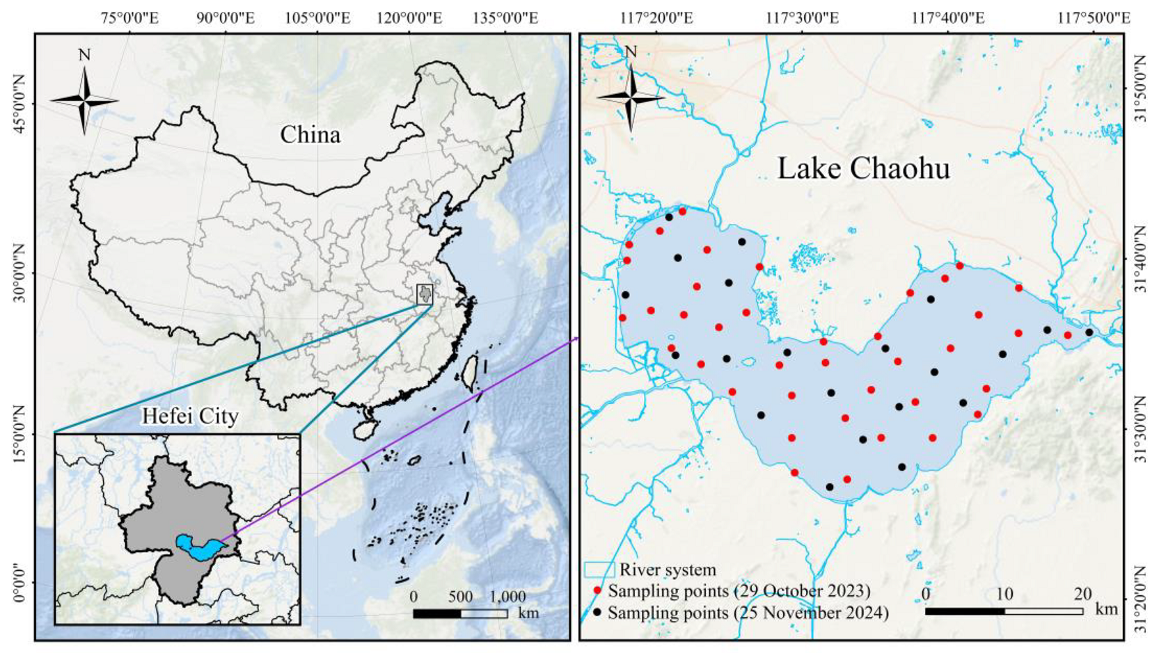
Figure 1. Location of the study area and distribution of sampling sites.
Applsci 15 08867 g001
Figure 2. Architecture of the CNN-based model. HSI refers to hyperspectral imagery. CONV denotes convolution operations, and FC Layer represents fully connected layers.
Applsci 15 08867 g002
Figure 3. Structure of the multi-head attention mechanism.
Applsci 15 08867 g003
Figure 4. Architecture of the CMAF-Net model.
Applsci 15 08867 g004
Figure 5. Workflow of DOC concentration prediction.
Applsci 15 08867 g005
Figure 6. Pearson correlation between DOC and satellite-derived hyperspectral variables, including single-band features (original reflectance and first-order derivative) and band-combination indices (DI, NDI, RI1, RI2, TBI).
Applsci 15 08867 g006
Figure 7. Correlation matrix of satellite single bands and band-combination indices used as input features for DOC modeling. Circle color indicates the direction and magnitude of Pearson correlation coefficients (blue for strong positive, red for strong negative), and the size of each circle is proportional to the absolute correlation value.
Applsci 15 08867 g007
Figure 8. Scatter plots showing the DOC prediction performance of the four models: (a) SVR, (b) RF, (c) CNN, and (d) CMAF-Net. The black dashed line represents the ideal reference line of a 1:1 ratio, while the solid red line indicates the regression trend line for each model.
Applsci 15 08867 g008aApplsci 15 08867 g008b
Figure 9. Radar plots illustrate the DOC prediction performance of four models across five-fold cross-validation. To ensure consistent interpretation, larger values indicate better performance, as the values of RMSE, MAE, and SMAPE are presented as reciprocals. The plots labeled Fold1 to Fold5 correspond to the results of the five individual validation folds, and the plot labeled Mean represents the average performance across all folds.
Applsci 15 08867 g009aApplsci 15 08867 g009b
Figure 10. DOC distribution maps predicted by four different models: (a) SVR, (b) RF, (c) CNN, and (d) CMAF-Net.
Applsci 15 08867 g010
Figure 11. Contribution analysis of individual spectral input features in the CMAF-Net model.
Applsci 15 08867 g011
Figure 12. Distribution of DOC and related factors at sampling sites in the eastern and western lakes. Black dots denote measured values, and red dots indicate flagged outliers. All values are expressed in mg/L.
Applsci 15 08867 g012
Figure 13. Correlation analysis of DOC and five influencing factors.
Applsci 15 08867 g013
Table 1. Statistical characteristics of DOC concentrations in water samples.
Sampling DateNumberMin
(mg/L)
Max
(mg/L)
Mean
(mg/L)
Standard
Deviation
IQR
29 October 2023393.539.034.401.110.76
25 November 2024213.845.704.480.480.46
Table 2. Hyperspectral sensor specifications of the ZY1-02D and ZY1-02E satellites.
Satellite PayloadZY1-02DZY1-02E
Launch date12 September 201926 December 2021
Number of spectral bands166166
Spectral range (nm)400–2500400–2500
Spectral resolution (nm)10(VNIR) 20(SWIR)10(VNIR) 20(SWIR)
Spatial resolution (m)3030
Swath width (km)6060
Revisit period (days)33
Table 3. Descriptive statistics of the sample set.
Sample SetNumberDOC Content (mg/L)
MinMaxMeanStandard Deviation
Training Set423.539.034.390.98
Test Set183.667.354.520.82
Total Set603.539.034.430.93
Table 4. Evaluation indicators of machine learning models in training and test sets.
Model TypeTraining SetTest Set
R2RMSERPDR2RMSERPD
SVR0.780.492.010.700.501.65
RF0.820.402.440.750.471.74
CNN0.870.323.070.820.362.30
CMAF-Net0.930.263.770.880.292.79
Table 5. Evaluation metrics of machine learning models on the validation set.
Model TypeValidation Set (CV-Score)
RMSERPDSMAPEMAER2
SVR0.741.3811.89%0.570.60 ± 0.06
RF0.631.519.49%0.450.68 ± 0.04
CNN0.501.969.13%0.420.76 ± 0.04
CMAF-Net0.452.187.78%0.350.81 ± 0.02
Disclaimer/Publisher’s Note: The statements, opinions and data contained in all publications are solely those of the individual author(s) and contributor(s) and not of MDPI and/or the editor(s). MDPI and/or the editor(s) disclaim responsibility for any injury to people or property resulting from any ideas, methods, instructions or products referred to in the content.