Article

Deep Learning-Based Vehicle Speed Estimation Using Smartphone Sensors in GNSS-Denied Environment

Division of Software, Hallym University, 1-Hallymdeahck-gil, Chuncheon 24252, Republic of Korea
*
Author to whom correspondence should be addressed.
Appl. Sci. 2025, 15(16), 8824; https://doi.org/10.3390/app15168824
Submission received: 16 June 2025 / Revised: 5 August 2025 / Accepted: 6 August 2025 / Published: 10 August 2025
(This article belongs to the Section Transportation and Future Mobility)

Abstract

This study presents a deep learning-based framework for vehicle speed estimation in GNSS-denied environments, such as underground parking lots, using only smartphone sensors. Accurate speed estimation in such environments is critical for enabling infrastructure-free indoor navigation, yet remains challenging due to sensor noise, orientation variability, and the lack of GNSS signals. The proposed model leverages accelerometer and gyroscope data without requiring transformation from the smartphone’s body frame to a global navigation frame, thereby simplifying the preprocessing pipeline. An LSTM network combined with an attention mechanism is employed to capture temporal dependencies in sequential sensor data. To improve estimation accuracy, statistical features are also incorporated. Training data were collected over a distance of 41.8 km using four smartphones in real-world parking lot environments. The model was further validated through controlled experiments under three test scenarios, including circular driving and repeated turning maneuvers. Across all scenarios, the proposed method achieved a mean RMSE of 0.38 m/s with consistent performance across different device orientations. These results demonstrate that the proposed approach achieves high speed estimation accuracy and robustness across various phone orientations, without the need for additional infrastructure. This highlights the potential of combining deep learning and smartphone sensing for reliable indoor navigation in challenging environments.

1. Introduction

In modern society, vehicles have become an essential part of daily life, with location information playing a crucial role in optimizing routes and maximizing efficiency. GNSS (Global Navigation Satellite System) enables precise vehicle positioning and has led to the active development of various application services [1]. However, GNSS signals cannot be received in indoor environments, making it difficult to apply outdoor navigation or ride-hailing services directly in such settings [2]. Although various studies have investigated methods for estimating vehicle positions in indoor environments, no system has yet been established that provides accuracy, convenience, and availability comparable to GNSS use outdoors. While some research employs WiFi [3,4,5,6], LTE signals [7,8] or a magnetic field [9,10,11] where GNSS cannot be received, it remains challenging to deliver GNSS-level accuracy on a large scale. BLE AOA [12] and UWB [13] can provide accuracy on the order of centimeters, yet they require infrastructure installation and dedicated receivers, posing significant drawbacks. Although many studies have explored vehicle positioning using cameras, their application to smartphones is still limited. [14,15,16].
This study proposes a deep learning-based method for accurate vehicle speed estimation in indoor environments using only smartphone-embedded sensors, such as accelerometers and gyroscopes, without the need for any additional hardware. The goal is to develop a system that can support precise indoor vehicle positioning—especially in GNSS-denied environments like underground parking lots—by providing reliable speed information derived solely from smartphone data. If such sensor-based speed estimation proves feasible, it can be effectively combined with radio frequency (RF) data to further enhance overall positioning accuracy. The proposed method employs a long short-term memory (LSTM) neural network, which is well-suited for modeling time-series data [17,18,19]. To enhance its ability to capture both short- and long-term temporal dependencies critical to speed estimation, an attention mechanism is incorporated between the LSTM layers and the fully connected output layer. This attention layer allows the model to selectively focus on the most relevant parts of the sensor sequence, thereby improving robustness and interpretability in complex driving conditions [20,21]. The model directly consumes raw sensor data recorded in the smartphone’s local body frame, avoiding the need to convert the data into a global navigation frame. Inspired by the feature learning capabilities of convolutional neural networks (CNNs) [22,23]—which automatically extract salient features from raw data using learnable filters—this study adopts a similar philosophy: instead of relying entirely on hand-engineered features, raw sensor data are input directly into the model so that relevant features for speed estimation can be learned through training. However, as handcrafted statistical features have shown strong performance in prior research [24], this study systematically compares multiple feature configurations: raw-only, statistical-only, and combined. Additionally, because the performance of LSTM models is sensitive to the input sequence length, the proposed method explores a range of sequence durations to empirically determine the optimal setting for various driving conditions.
The remainder of this paper is organized as follows: Section 2 presents related works. Section 3 describes the proposed radio map and localization algorithm. Section 4 presents the experimental results. Finally, Section 5 concludes the paper.

2. Related Works

Dead Reckoning (DR) is a navigation technique that estimates position by integrating acceleration data from an inertial measurement unit (IMU) to compute velocity and position, while using gyroscope data to track changes in orientation over time from an initial known position [25]. This method operates independently of external signals, making it effective in GPS-denied environments such as indoor navigation, autonomous vehicles, and underwater systems. However, since sensor errors accumulate over time, DR inherently suffers from drift, which necessitates periodic correction using external references such as GPS or Wi-Fi. To mitigate this drift and improve positioning accuracy, Kalman filtering (KF) is commonly employed to fuse DR outputs with external data [26]. Despite these limitations, DR remains a critical component in various applications, including robotics [27], aerospace [28], and military navigation [29]. Table 1 presents a list of studies on artificial intelligence-based vehicle positioning. Freydin [30] proposed a method that leverages low-cost IMU data to train a deep neural network (DNN) model for vehicle speed estimation, which is then used as a pseudo-measurement for Dead Reckoning. Specifically, an LSTM architecture was adopted to learn temporal dependencies in IMU data, significantly reducing positioning errors compared to conventional acceleration integration-based methods. The study showed that combining the model with traditional sensor fusion techniques such as KF improved the accuracy of DR-based navigation in GNSS-denied environments. Gao [31] introduced VeTorch, a smartphone-based vehicle tracking framework designed to mitigate accumulated errors from low-quality IMU sensors in GPS-denied environments. The proposed approach integrates an inertial sequence learning framework to enhance real-time vehicle tracking performance. To handle arbitrary smartphone placement, a motion transformation algorithm was applied, and a temporal convolutional network (TCN)-based sequence model was adopted to reduce the accumulated errors inherent in DR. Moreover, federated learning was employed to train personalized models for individual smartphones, enabling the system to adapt to varying smartphone characteristics and driving styles. Zhou [32] proposed DeepVIP, a deep learning-based indoor vehicle positioning model to improve accuracy in GNSS-denied environments. While traditional methods often rely on infrastructure-based solutions such as Wi-Fi or BLE—or suffer from cumulative drift due to limitations in low-cost IMU sensors—DeepVIP addresses these challenges by utilizing integrated smartphone sensors including accelerometers, gyroscopes, magnetometers, and gravity sensors. Two versions were introduced: DeepVIP-L, an LSTM-based model targeting high-accuracy applications, and DeepVIP-M, a lightweight MobileNet-V3-based model designed for computational efficiency. Experimental results showed that DeepVIP outperformed existing data-driven inertial navigation methods, achieving accurate localization without requiring additional infrastructure. Tong [33] proposed a novel inertial learning framework for smartphone-based vehicle tracking in GPS-denied environments. Conventional DR-based approaches suffer from degraded accuracy due to smartphone placement variability, high sensor noise, and device-specific differences. To overcome these challenges, the study applied a PCA-based coordinate transformation algorithm to align the smartphone with the vehicle’s reference frame. In addition, a TCN-based sequence learning model was used to reduce error accumulation, and a personalized retraining strategy was introduced to further adapt to individual smartphones and driving behaviors. The approach was implemented on the DiDi platform, where real-world evaluations confirmed its effectiveness in practical vehicle tracking scenarios.
Unlike prior works requiring coordinate transformation or personalized model retraining, our method directly uses raw IMU data in the smartphone’s body frame without alignment. Despite minimal preprocessing, it achieves high accuracy by combining raw and handcrafted features. The attention-based LSTM architecture further enhances temporal learning. No additional infrastructure is needed, making the system practical and scalable. This simplicity ensures strong generalization across devices and driving conditions.

3. Proposed System

In this study, a deep learning model is employed to estimate vehicle speed using only smartphone sensors. To enhance the model’s ability to capture temporal dependencies, an attention mechanism is incorporated between the LSTM and fully connected layers. A key aspect of this work is the investigation of whether accurate speed estimation can be achieved without transforming the sensor data from the smartphone’s local body frame to a global navigation frame. By directly utilizing raw sensor inputs in the body frame, the study aims to evaluate the practicality and generalization capability of the proposed model in real-world driving environments, thereby minimizing preprocessing requirements while maintaining high prediction accuracy.

3.1. LSTM with Attention Layer

LSTM is a recurrent neural network (RNN) variant designed to capture long-term dependencies in sequential data [34]. Traditional RNNs suffer from vanishing and exploding gradient problems, making them ineffective for learning from long time-series data. LSTMs address this limitation by introducing a memory cell structure that selectively retains and forgets information through three key gates: the forget gate, which determines which past information should be discarded, the input gate, which decides how much new information to store, and the output gate, which regulates the amount of information passed to the next time step. This gated mechanism enables stable gradient propagation, allowing LSTMs to process long sequences effectively. In this study, LSTM is utilized to estimate vehicle speed using only smartphone sensor data, eliminating reliance on external sources such as GPS or OBD2. Instead of manually engineering features, the model directly processes raw sensor inputs, allowing deep learning to automatically extract meaningful representations for speed estimation. Also, previous research suggests that handcrafted features can still provide valuable information, so this study systematically evaluates the effectiveness of different combinations of raw and engineered features. To further enhance performance, an attention layer is integrated into the LSTM architecture [35]. Traditional LSTMs process all time steps equally, but an attention mechanism assigns dynamic weights to each input, enabling the model to focus on the most relevant time steps for speed estimation. This reduces the impact of irrelevant or noisy data and helps mitigate long-term dependency issues. By placing the attention layer between the LSTM and fully connected layers, the model learns to emphasize key temporal patterns that contribute most significantly to accurate speed estimation. Each input sequence of smartphone sensor data is paired with the corresponding ground truth speed measured by the OBD2 interface, enabling supervised learning. This one-to-one mapping between input and target allows the model to directly learn the relationship between temporal sensor patterns and true vehicle speed. Through this end-to-end training process, the model can extract complex dependencies that are difficult to capture with manual feature engineering or rule-based approaches.
Figure 1 illustrates the architecture of the proposed speed estimation model. The input to the network is a fixed-length sequence of sensor vectors, denoted as X like
X = x ¯ 1 , x ¯ 2 , x ¯ T R T × D ,
where T represents the sequence length and D denotes the number of sensor features per time step. The sequential input is first passed through two stacked LSTM layers. The first LSTM layer with 64 hidden units produces a hidden representation sequence, H 1 R T × 64 , which is then passed to the second LSTM layer. The second layer reduces the dimensionality to 32, resulting in H 2 R T × 32 , used as the input to the self-attention module. To enable the model to focus on informative time steps, a self-attention mechanism is applied. The attention weights are computed as
A t t e n t i o n ( Q , K , V ) = s o f t   max ( Q K T 32 ) V ,
where Q , K , and V R T × 32 are query, key, and value matrices, respectively. These matrices are calculated as
Q = H 2 W Q ,
K = H 2 W K ,
V = H 2 W V ,
where W Q , W K , and W V R 32 × 32 are learnable weight matrices that project the input sequence into query, key, and value representations, respectively. The output of the attention layer is concatenated with the output of the second LSTM layer, and the resulting sequence is subsequently aggregated via a pooling operation to form a context vector, c ¯ . Finally, this vector is passed through fully connected layers to estimate the target speed v .

3.2. LSTM Input

To construct the input data for the LSTM model, we used a sequence of T time steps, where each time step is represented by a 21-dimensional feature vector. These feature vectors consist of raw sensor measurements along with statistical features such as mean and variance, extracted from the raw data. The raw sensor data consist of acceleration values along the x, y, and z axes, gyroscope values along the x, y, and z axes, and the norm of the acceleration vector.
Magnetometer readings were not included, as they are highly sensitive to environmental disturbances in indoor spaces and tend to degrade the model’s stability and performance [36,37]. In addition to the raw sensor values, statistical features were extracted from each axis of the accelerometer and gyroscope. For each T-length input sequence, we computed the mean and variance of the signal over the sequence using the following equations
μ = 1 T i = 1 T x i ,
σ 2 = 1 T 1 i = 1 T ( x i μ ) 2
We use sample variance rather than population variance because the statistical features are computed over relatively short sequences (e.g., 1–5 s) in real-time conditions. As a result, each input vector includes 7 features from the raw sensor data and 14 features derived from the statistical summaries, leading to a total of 21 elements per time step. These features are concatenated to form an input matrix of size T by 21, which is then fed into the LSTM network for training and inference.

4. Experimental Results

4.1. Experimental Setting and Scenario

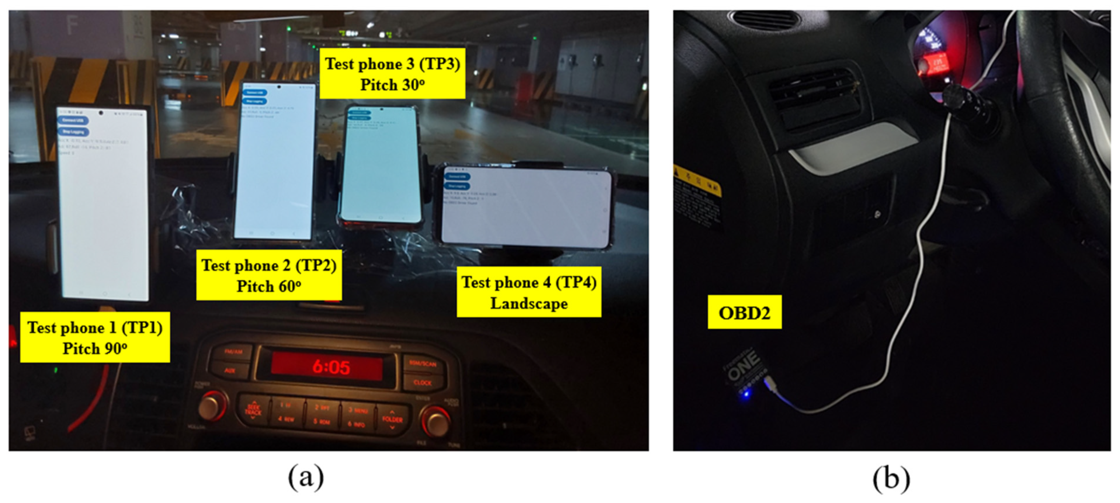
We conducted experiments on the third basement level of the Emart underground parking lot in Seoul, South Korea, to evaluate the effectiveness of speed estimation using smartphone sensor data under various device orientations. The parking lot measures approximately 180 m in length and 80 m in width, with a single entrance and exit. Four smartphones—two Samsung Galaxy S22 Ultra and two Galaxy S20—were mounted inside a vehicle using phone holders to simulate realistic navigation scenarios. To reflect practical variations in smartphone placement, data were collected under four orientations: three pitch angles of 90°, 60°, and 30°, and landscape mode, as illustrated in Figure 2a. The recorded data included accelerometer, gyroscope, magnetometer, and barometric pressure readings, along with estimated motion parameters such as yaw, roll, and pitch. Additionally, vehicle speed was collected via OBD2 and logged in parallel as reference data for supervised learning. All signals were sampled at 50 Hz and stored in CSV format for further analysis. Prior to the evaluation scenarios, extensive data collection was conducted in an underground parking lot using four smartphones, which were freely moved to cover a wide range of trajectories. Approximately 42 min of continuous sensor data were collected, resulting in a total traveled distance of about 41.8 km. This dataset was used for model training. To validate the trained model, additional experiments were conducted under three distinct test scenarios. The first and second scenarios involved counterclockwise driving around the parking lot, while the third scenario consisted of repeated turning maneuvers. Figure 3 illustrates the vehicle trajectories corresponding to each experimental scenario. In Scenarios 1 and 2, the vehicle followed a counterclockwise route along a rectangular path, whereas in Scenario 3, the vehicle repeatedly performed turning maneuvers to simulate complex driving behavior. The red dot and red arrow in each subfigure represent the starting position and initial driving direction, respectively. Figure 4 shows the ground truth velocity profiles obtained from the OBD2 device for each scenario. The speed profiles reflect differences in driving patterns, with more frequent acceleration and deceleration observed in Scenario 3 due to the continuous turning motion.
Data processing was performed using Google Colab, and figures were generated using MATLAB R2019b.

4.2. Model Architecture Overview and Training Configuration

Prior to model training, the sensor data underwent several preprocessing steps. All signals were first normalized using min-max scaling to ensure numerical stability. The resulting sequences were then segmented into fixed-length windows suitable for input to the model. As illustrated in Figure 1, the model consists of two stacked LSTM layers followed by a self-attention mechanism, which is used to emphasize informative time steps. The attention output is concatenated with the LSTM output and aggregated via temporal pooling. The resulting context vector is then passed through a fully connected layer to predict the vehicle speed. The model was trained using an Adam optimizer with an initial learning rate of 0.0008. To improve convergence when the validation loss plateaued, an adaptive learning rate scheduler was employed to reduce the learning rate by a factor of 0.5 after five epochs without improvement, with a minimum rate of 1 × 10⁻⁶.

4.3. Model Performance Analysis

To evaluate model performance, we employed three commonly used regression metrics: Root Mean Squared Error (RMSE) and Mean Absolute Error (MAE). RMSE measures the square root of the average squared differences between predicted and actual values, indicating overall prediction accuracy. MAE quantifies the average absolute error across all predictions, providing an intuitive measure of typical prediction error. Maximum Error captures the largest absolute deviation between predicted and true values, highlighting the model’s worst-case performance.

4.3.1. Comparison of Model Performance Using Different Feature Inputs

Table 2 and Table 3 present the model’s prediction performance under different feature inputs, and smartphone orientations. An analysis of the performance with respect to the sequence length is provided in Appendix A. The results demonstrate that the combination of raw sensor features and statistical features consistently led to the most accurate and stable predictions across various test scenarios. When using raw sensor data, the model showed its best performance at a sequence length of 200 (4 s). In first and second scenarios, the pitch 90° orientation produced the lowest RMSE values, indicating stable signal patterns under that orientation. In contrast, in the third scenario, which involved frequent turns and dynamic motion, the pitch 60° orientation outperformed all others. As the sequence length increased beyond 300, the performance generally declined across all orientations, likely due to the accumulation of noise and redundant information. When statistical features (mean and variance) were used alone, overall prediction accuracy decreased, and RMSE values increased across all test conditions. The performance drop was particularly evident in the third scenario, where rapid changes in motion were poorly represented by aggregated features. Although the optimal sequence length was still around 200, the models showed higher sensitivity to time window variations and greater instability compared to the raw feature setting. In contrast, using combined features significantly improved robustness and generalization. Across all tests, the combined feature model consistently achieved the lowest RMSE and MAE values at a 200-length sequence. Notably, the performance remained relatively stable across different sequence lengths, indicating greater tolerance to temporal scale variation. In simpler paths like first and second scenarios, pitch 90° again yielded the best results. However, in the third scenario, pitch 60° clearly outperformed the other orientations, reinforcing its advantage in dynamic environments. In all settings, the pitch 30° orientation performed the worst. The landscape orientation showed moderate performance but was generally inferior to pitch 60°, particularly under turning scenarios.
Across all feature types, the 4 s sequence length consistently produced the best trade-off between capturing temporal information and reducing overfitting or noise. In summary, the combined feature model with a 4 s sequence length achieved the most accurate and stable results. Pitch 90° was most effective in regular driving paths, while pitch 60° proved more suitable for complex, high-variation scenarios. The results highlight the importance of both feature selection and sequence configuration for reliable speed estimation using smartphone sensor data. Figure 5 illustrates the error distributions across four test points (TP1–TP4) under three different feature settings: (a) raw features, (b) statistical features, and (c) combined features. All results use a fixed sequence length of 200, and both histogram and kernel density estimation curves are provided to visualize the spread and shape of the error distribution. TP1 consistently exhibits narrow and symmetric distributions, indicating stable estimation, whereas TP3 and TP4 show heavier tails and broader spreads, particularly under more complex scenarios. Among the three settings, the combined feature set in (c) achieves the sharpest and most concentrated distributions across all test points, suggesting superior overall performance.

4.3.2. Model Performance Using All Feature Types (Raw + Statistical) with a Sequence Length of 200

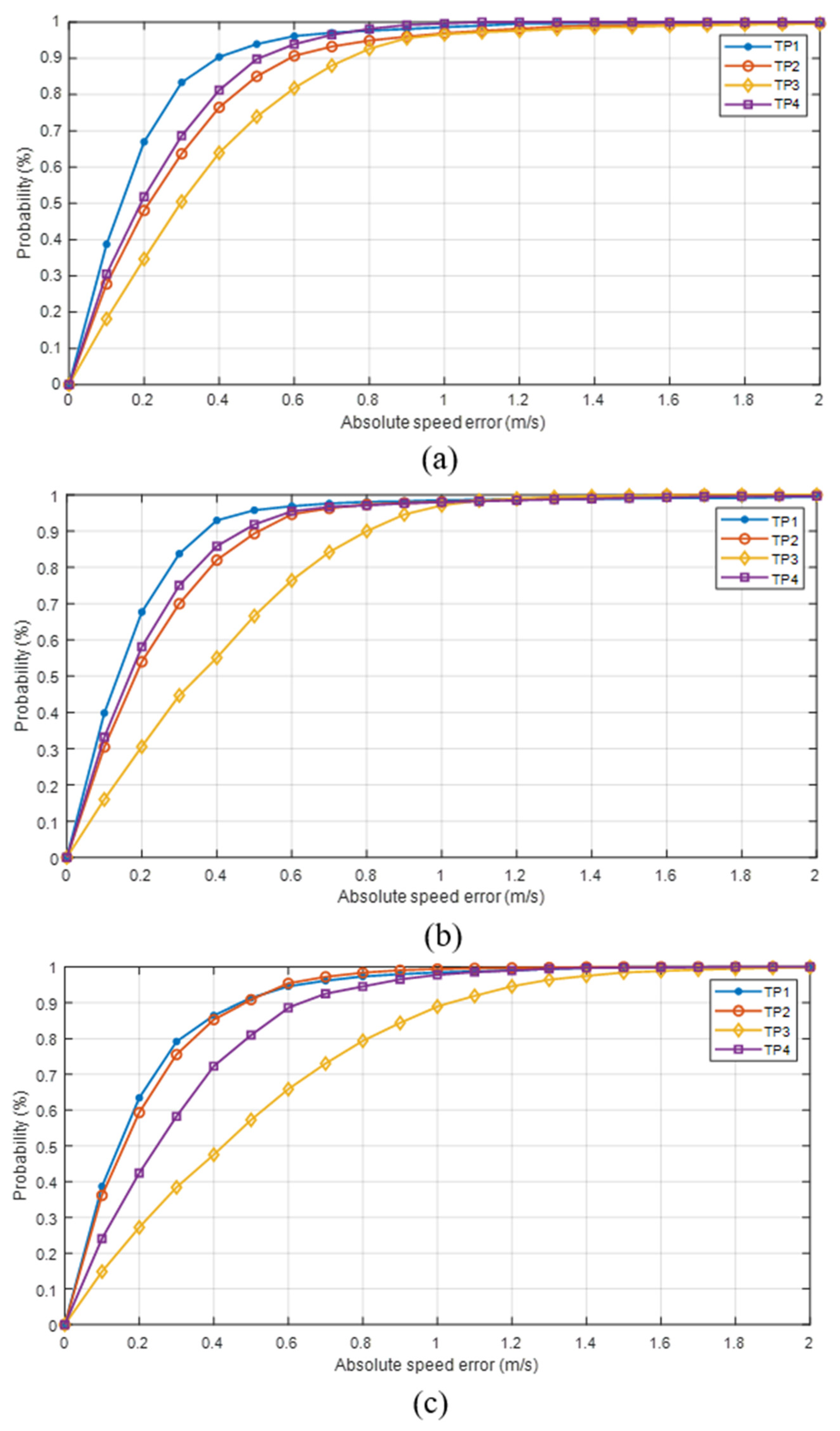
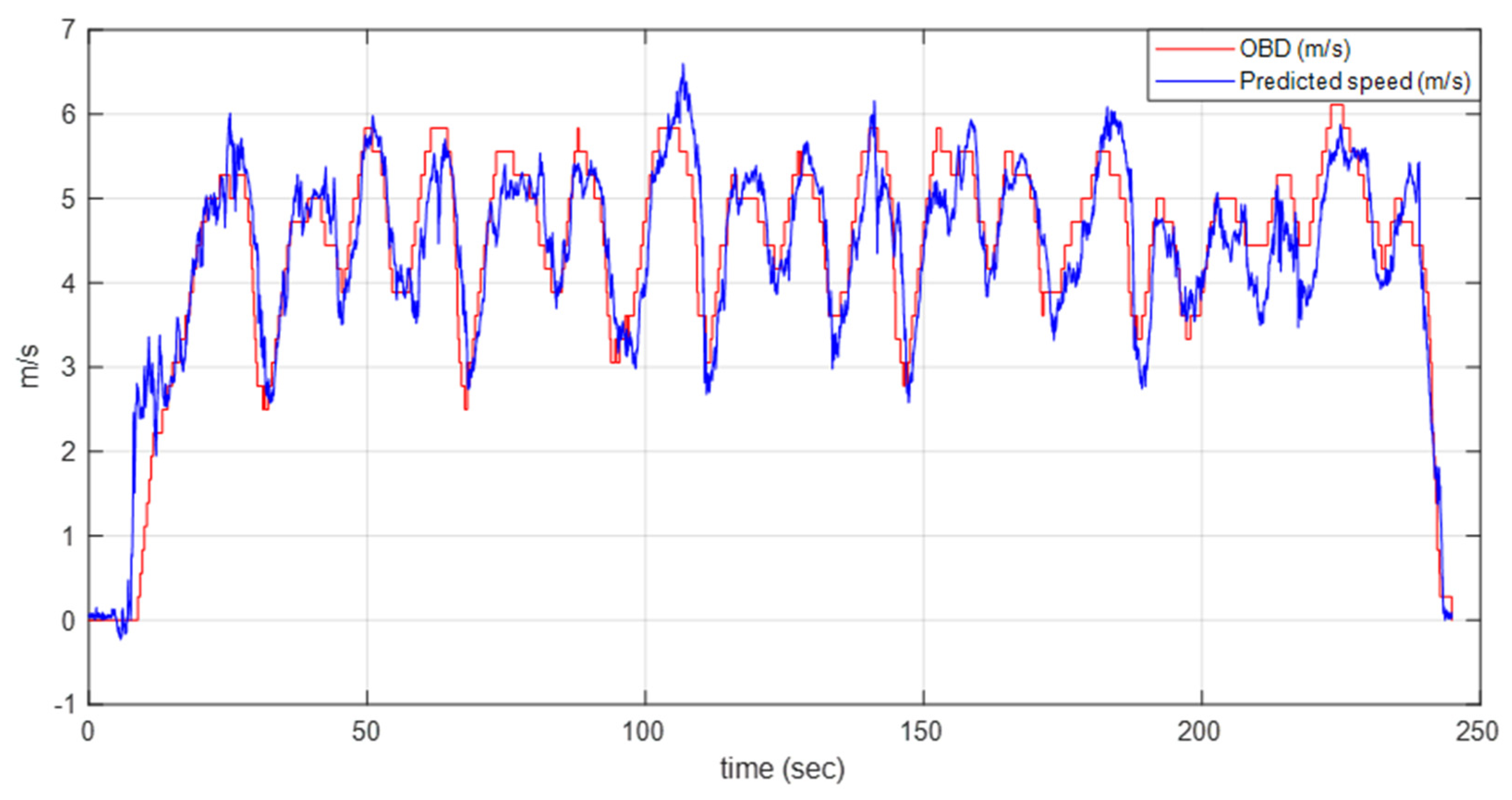
To further evaluate the model’s performance, we analyzed the cumulative distribution function (CDF) of RMSE using the optimal configuration: a sequence length of 200 (4 s) and all features (raw + statistical). Figure 6 presents the CDF curves of prediction errors across the first, second, and third scenarios, corresponding to subfigures (a), (b), and (c), respectively. In the first and second scenarios, which involved controlled closed-loop driving, the pitch 90° orientation consistently exhibited the best performance, as shown by its steep CDF curves that quickly reach saturation. This indicates that most of the prediction errors remain within a small range. The pitch 60° orientation followed closely, offering relatively stable accuracy. In the third scenario, which featured complex figure-eight driving and frequent speed changes, the pitch 60° orientation slightly outperformed pitch 90° in certain error ranges, suggesting greater adaptability to dynamic motion. However, pitch 90° still maintained strong overall accuracy. The pitch 30° consistently resulted in the widest error distribution, indicating that it is less reliable under unstable driving conditions. Comparisons with models using only statistical features (Appendix A) revealed a significant drop in accuracy, especially under complex motion. However, when both raw and statistical features were used together, the model maintained robust performance across all scenarios. This highlights the importance of feature fusion in ensuring generalization and error resilience. In summary, the CDF analysis confirms that the pitch 90° orientation with a 4 s sequence length yields the most stable and accurate predictions. The pitch 60° orientation proves particularly effective in dynamic environments, and the integration of both feature types significantly enhances model robustness. To empirically verify the reliability of the proposed model, we compared the predicted vehicle speed with the ground truth obtained from the OBD2 system under the first scenario, using all features and the pitch 90° orientation, which previously demonstrated the best performance. As illustrated in Figure 7, the predicted speed curve shows strong agreement with the actual OBD2 data. The model successfully captures both gradual and rapid changes in velocity, including acceleration and deceleration segments. This close alignment serves as concrete evidence that the model is capable of accurately estimating real vehicle speed using only smartphone sensor data. This result validates the model’s practical utility and supports its potential application in GNSS-denied environments, where direct access to vehicle velocity may not be available.

4.4. Discussion

This study explored a smartphone-based vehicle speed estimation method using only inertial sensor data in GNSS-denied environments. Experiments were conducted in an underground parking lot under various device orientations and driving scenarios to assess the robustness of the proposed model. By combining raw sensor inputs with statistical features, and employing an LSTM network enhanced with self-attention, the model effectively captured temporal dependencies and adapted to diverse motion patterns. Table 4 presents a performance comparison between the proposed method and existing approaches, including KF-based and DNN-based models. In the case of KF, speed was estimated by integrating inertial measurements with GNSS data based on a physical motion model. In contrast, our method operates under GNSS-denied conditions, without any satellite-based positioning input. Although experimental setups and devices differ across studies, the results suggest that our method achieves slightly better accuracy, highlighting its effectiveness even in more constrained environments.
However, the current evaluation was conducted in a single underground parking facility, which limits the generalizability of the findings. This limitation has been explicitly acknowledged, and future work will involve conducting experiments across diverse indoor environments to assess the model’s adaptability. To enhance generalization, the proposed method excludes magnetometer data, which are highly sensitive to surrounding infrastructure and electromagnetic interference in indoor environments. By relying solely on accelerometer and gyroscope measurements, the model becomes less affected by environmental variability. Nonetheless, this design assumption should be validated through further testing in structurally different environments.

5. Conclusions

This study proposed a deep learning-based vehicle speed estimation framework utilizing only smartphone sensors, specifically targeting GNSS-denied environments such as underground parking facilities. By integrating an LSTM network with an attention mechanism and combining raw sensor data with hand-crafted features, the model effectively captured temporal dynamics and enhanced estimation accuracy. Experimental results demonstrated that a 4 s sequence length yielded optimal performance across various smartphone orientations, with the pitch 90° posture showing the highest accuracy in general scenarios and pitch 60° exhibiting superior robustness under complex driving conditions. The combined feature input consistently outperformed individual input types in terms of both accuracy and stability. Notably, the proposed approach requires no additional infrastructure, offering a cost-effective and scalable solution for indoor vehicular navigation. The key contributions of this study include (1) a sensor-only speed estimation framework robust to device orientation changes, (2) a feature fusion strategy combining raw and statistical inputs, and (3) extensive validation across diverse driving scenarios. However, the study has several limitations that should be addressed in future work. Device variability, such as differences in sensor quality across smartphone models, may affect model performance. Additionally, sensor noise and potential model drift during long-term deployments could influence estimation accuracy in practical scenarios. These factors will be systematically investigated in follow-up studies. The proposed framework may be applicable to various indoor mobility applications, such as underground navigation for autonomous vehicles, smartphone-based speed tracking in large indoor venues, or integration with RF-based localization systems for more robust positioning.

Author Contributions

Conceptualization, B.S. and S.L.; methodology, S.L. and B.K.; software, S.L. and B.K.; validation, S.L. and B.K.; formal analysis, B.S.; investigation, B.S.; resources, B.S.; writing—original draft preparation, B.S. and S.L.; writing—review and editing, B.S.; funding acquisition, B.S. All authors have read and agreed to the published version of the manuscript.

Funding

This research was supported by Hallym University Research Fund, 2025 (HRF-202501-006).

Institutional Review Board Statement

Not applicable.

Informed Consent Statement

Not applicable.

Data Availability Statement

Derived data supporting the findings of this study are available from the corresponding author on request. The data are not publicly available due to privacy.

Conflicts of Interest

The authors declare no conflicts of interest.

Appendix A

The tables below present the complete experimental results for each scenario, showing the effects of sequence length and device orientation for each feature configuration.
Table A1. Model performance evaluation of RMSE and MAE with raw features.
TScenarioTP1 RMSE (m/s)TP1 MAE (m/s)TP2 RMSE (m/s)TP2 MAE (m/s)TP3 RMSE (m/s)TP3 MAE (m/s)TP4 RMSE (m/s)TP4 MAE (m/s)
100First0.310.230.490.340.70.50.510.38
Second0.360.260.410.310.650.490.410.29
Third0.330.240.350.260.830.620.430.31
200First0.320.230.400.290.490.370.420.31
Second0.400.210.350.260.470.360.340.24
Third0.380.280.310.240.690.560.380.30
300First0.360.230.360.260.520.390.410.29
Second0.340.220.370.270.540.420.380.28
Third0.440.270.320.240.710.560.390.29
400First0.380.290.450.330.530.390.430.32
Second0.450.290.420.290.520.380.460.31
Third0.430.330.40.280.730.570.510.37
500First0.290.190.330.270.570.420.460.31
Second0.590.290.440.280.530.40.570.32
Third0.410.310.440.320.760.60.60.39
Table A2. Model performance evaluation of RMSE and MAE with statistical features.
TScenarioTP1 RMSE (m/s)TP1 MAE (m/s)TP2 RMSE (m/s)TP2 MAE (m/s)TP3 RMSE (m/s)TP3 MAE (m/s)TP4 RMSE (m/s)TP4 MAE (m/s)
100First0.510.350.760.560.460.340.780.5
Second0.520.370.710.530.470.340.480.35
Third0.570.40.850.660.430.30.550.36
200First0.340.240.570.400.560.390.700.44
Second0.430.280.470.310.500.400.500.36
Third0.400.280.440.290.710.570.450.34
300First0.360.260.620.460.610.40.510.36
Second0.50.310.640.470.50.320.480.32
Third0.420.270.820.630.40.290.60.42
400First0.480.370.620.460.770.540.580.46
Second0.550.40.770.540.750.510.590.43
Third0.620.4510.730.690.460.810.59
500First0.480.370.810.520.630.450.580.44
Second0.530.420.740.510.650.470.660.45
Third0.610.490.890.670.610.470.930.65
Table A3. Model performance evaluation of RMSE and MAE with combined features.
TScenarioTP1 RMSE (m/s)TP1 MAE (m/s)TP2 RMSE (m/s)TP2 MAE (m/s)TP3 RMSE (m/s)TP3 MAE (m/s)TP4 RMSE (m/s)TP4 MAE (m/s)
100First0.330.220.70.530.480.330.460.33
Second0.320.210.570.440.370.280.40.29
Third0.320.220.740.570.330.250.390.29
200First0.280.190.410.290.490.370.310.24
Second0.300.190.340.240.490.400.340.23
Third0.300.210.290.210.630.500.400.30
300First0.290.20.440.330.380.290.340.28
Second0.370.230.510.390.380.260.370.23
Third0.420.30.690.550.350.260.410.31
400First0.280.20.520.40.350.270.320.26
Second0.380.220.560.420.460.30.440.29
Third0.440.310.80.60.490.320.550.36
500First0.330.20.60.440.420.320.40.35
Second0.610.240.610.410.510.290.460.27
Third0.410.260.810.630.550.360.570.37

References

  1. Zhu, N.; Marais, J.; Betaille, D.; Berbineau, M. GNSS Position Integrity in Urban Environments: A Review of Literature. IEEE Trans. Intell. Transp. Syst. 2018, 19, 2762–2778. [Google Scholar] [CrossRef]
  2. Shin, B.; Lee, J.H.; Yu, C.; Kim, C.; Lee, T. Underground parking lot navigation system using long-term evolution signal. Sensors 2021, 21, 1725. [Google Scholar] [CrossRef] [PubMed]
  3. Álvarez-Merino, C.S.; Luo-Chen, H.Q.; Khatib, E.J.; Barco, R. WiFi FTM, UWB and Cellular-Based Radio Fusion for Indoor Positioning. Sensors 2021, 21, 7020. [Google Scholar] [CrossRef] [PubMed]
  4. Luo, J.; Zhang, Z.; Wang, C.; Liu, C.; Xiao, D. Indoor Multifloor Localization Method Based on WiFi Fingerprints and LDA. IEEE Trans. Ind. Inform. 2019, 15, 5225–5234. [Google Scholar] [CrossRef]
  5. Sun, C.; Zhou, J.; Jang, K.; Kim, Y. Indoor Localization Based on Integration of Wi-Fi with Geomagnetic and Light Sensors on an Android Device Using a DFF Network. Electronics 2023, 12, 5032. [Google Scholar] [CrossRef]
  6. Jin, S.; Kim, D. WiFi Fingerprint Indoor Localization Employing Adaboost and Probability-One Access Point Selection for Multi-Floor Campus Buildings. Future Internet 2024, 16, 466. [Google Scholar] [CrossRef]
  7. Lee, J.-H.; Shin, B.; Shin, D.; Kim, J.; Park, J.; Lee, T. Precise Indoor Localization: Rapidly-Converging 2D Surface Correlation-Based Fingerprinting Technology Using LTE Signal. IEEE Access 2020, 8, 172829–172838. [Google Scholar] [CrossRef]
  8. Jeon, J.; Ji, M.; Lee, J.; Han, K.-S.; Cho, Y. Deep Learning-Based Emergency Rescue Positioning Technology Using Matching-Map Images. Remote Sens. 2024, 16, 4014. [Google Scholar] [CrossRef]
  9. Shin, B.; Lee, J.-H.; Yu, C.; Kyung, H.; Lee, T. Magnetic Field-Based Vehicle Positioning System in Long Tunnel Environment. Appl. Sci. 2021, 11, 11641. [Google Scholar] [CrossRef]
  10. Yu, N.; Chen, X.; Feng, R.; Wu, Y. High-Precision Pedestrian Indoor Positioning Method Based on Inertial and Magnetic Field Information. Sensors 2025, 25, 2891. [Google Scholar] [CrossRef]
  11. Lu, Y.; Wei, D.; Li, W.; Ji, X.; Yuan, H. A Map-Aided Fast Initialization Method for the Magnetic Positioning of Vehicles. Electronics 2024, 13, 1315. [Google Scholar] [CrossRef]
  12. Huang, C.; Zhuang, Y.; Liu, H.; Li, J.; Wang, W. A Performance Evaluation Framework for Direction Finding Using BLE AoA/AoD Receivers. IEEE Internet Things J. 2021, 8, 3331–3345. [Google Scholar] [CrossRef]
  13. Wang, F.; Tang, H.; Chen, J. Survey on NLOS Identification and Error Mitigation for UWB Indoor Positioning. Electronics 2023, 12, 1678. [Google Scholar] [CrossRef]
  14. Rodríguez-Rangel, H.; Morales-Rosales, L.A.; Imperial-Rojo, R.; Roman-Garay, M.A.; Peralta-Peñuñuri, G.E.; Lobato-Báez, M. Analysis of Statistical and Artificial Intelligence Algorithms for Real-Time Speed Estimation Based on Vehicle Detection with YOLO. Appl. Sci. 2022, 12, 2907. [Google Scholar] [CrossRef]
  15. Wang, Z.; Huang, X.; Hu, Z. Attention-Based LiDAR–Camera Fusion for 3D Object Detection in Autonomous Driving. World Electr. Veh. J. 2025, 16, 306. [Google Scholar] [CrossRef]
  16. Tan, K.; Wu, J.; Zhou, H.; Wang, Y.; Chen, J. Integrating Advanced Computer Vision and AI Algorithms for Autonomous Driving Systems. J. Theory Pract. Eng. Sci. 2024, 4, 41–48. [Google Scholar] [CrossRef]
  17. Shu, Y.-H.; Chang, Y.-H.; Lin, Y.-Z.; Chow, C.-W. Real-Time Indoor Visible Light Positioning (VLP) Using Long Short Term Memory Neural Network (LSTM-NN) with Principal Component Analysis (PCA). Sensors 2024, 24, 5424. [Google Scholar] [CrossRef]
  18. Zhang, M.; Jia, J.; Chen, J.; Yang, L.; Guo, L.; Wang, X. Real-time indoor localization using smartphone magnetic with LSTM networks. Neural Comput. Appl. 2021, 33, 10093–10110. [Google Scholar] [CrossRef]
  19. Zhang, M.; Jia, J.; Chen, J.; Deng, Y.; Wang, X.; Aghvami, A.H. Indoor Localization Fusing WiFi With Smartphone Inertial Sensors Using LSTM Networks. IEEE Internet Things J. 2021, 8, 13608–13623. [Google Scholar] [CrossRef]
  20. Wu, Z.; Hu, P.; Liu, S.; Pang, T. Attention Mechanism and LSTM Network for Fingerprint-Based Indoor Location System. Sensors 2024, 24, 1398. [Google Scholar] [CrossRef]
  21. Deng, J.; Zhang, S.; Ma, J. Self-Attention-Based Deep Convolution LSTM Framework for Sensor-Based Badminton Activity Recognition. Sensors 2023, 23, 8373. [Google Scholar] [CrossRef]
  22. Yoon, J.-h.; Kim, H.-j.; Lee, D.-s.; Kwon, S.-k. Indoor Positioning Method by CNN-LSTM of Continuous Received Signal Strength Indicator. Electronics 2024, 13, 4518. [Google Scholar] [CrossRef]
  23. Lu, H.; Liu, S.; Hwang, S.-H. Local Batch Normalization-Aided CNN Model for RSSI-Based Fingerprint Indoor Positioning. Electronics 2025, 14, 1136. [Google Scholar] [CrossRef]
  24. Pei, L.; Liu, J.; Guinness, R.; Chen, Y.; Kuusniemi, H.; Chen, R. Using LS-SVM Based Motion Recognition for Smartphone Indoor Wireless Positioning. Sensors 2012, 12, 6155–6175. [Google Scholar] [CrossRef]
  25. Chu, T.; Guo, N.; Backén, S.; Akos, D. Monocular Camera/IMU/GNSS Integration for Ground Vehicle Navigation in Challenging GNSS Environments. Sensors 2012, 12, 3162–3185. [Google Scholar] [CrossRef] [PubMed]
  26. Chiang, K.-W.; Lin, C.-A.; Duong, T.-T. The Performance Analysis of the Tactical Inertial Navigator Aided by Non-GPS Derived References. Remote Sens. 2014, 6, 12511–12526. [Google Scholar] [CrossRef]
  27. Wei, X.; Li, P.; Tian, W.; Wei, D.; Zhang, H.; Liao, W.; Cao, Y. A fast dynamic pose estimation method for vision-based trajectory tracking control of industrial robots. Measurement 2024, 231, 114506. [Google Scholar] [CrossRef]
  28. Marinescu, M.; Olivares, A.; Staffetti, E.; Sun, J. On the Estimation of Vector Wind Profiles Using Aircraft-Derived Data and Gaussian Process Regression. Aerospace 2022, 9, 377. [Google Scholar] [CrossRef]
  29. Fontana, S.; Di Lauro, F. An Overview of Sensors for Long Range Missile Defense. Sensors 2022, 22, 9871. [Google Scholar] [CrossRef] [PubMed]
  30. Freydin, M.; Or, B. Learning car speed using inertial sensors for dead reckoning navigation. IEEE Sens. Lett. 2022, 6, 1–4. [Google Scholar] [CrossRef]
  31. Gao, R.; Xiao, X.; Zhu, S.; Xing, W.; Li, C.; Liu, L.; Ma, L.; Chai, H. Glow in the dark: Smartphone inertial odometry for vehicle tracking in GPS blocked environments. IEEE Internet Things J. 2021, 8, 12955–12967. [Google Scholar] [CrossRef]
  32. Zhou, B.; Gu, Z.; Gu, F.; Wu, P.; Yang, C.; Liu, X.; Li, L.; Li, Y.; Li, Q. DeepVIP: Deep learning-based vehicle indoor positioning using smartphones. IEEE Trans. Veh. Technol. 2022, 71, 13299–13309. [Google Scholar] [CrossRef]
  33. Tong, Y.; Zhu, S.; Ren, X.; Zhong, Q.; Tao, D.; Li, C.; Liu, L.; Gao, R. Vehicle Inertial Tracking via Mobile Crowdsensing: Experience and Enhancement. IEEE Trans. Instrum. Meas. 2022, 71, 2505513. [Google Scholar] [CrossRef]
  34. Staudemeyer, R.C.; Morris, E.R. Understanding LSTM—A Tutorial into Long Short-Term Memory Recurrent Neural Networks. arXiv 2019, arXiv:1909.09586. [Google Scholar]
  35. Wen, X.; Li, W. Time Series Prediction Based on LSTM-Attention-LSTM Model. IEEE Access 2023, 11, 48322–48331. [Google Scholar] [CrossRef]
  36. Ouyang, G.; Abed-Meraim, K. Analysis of Magnetic Field Measurements for Indoor Positioning. Sensors 2022, 22, 4014. [Google Scholar] [CrossRef]
  37. Ashraf, I.; Zikria, Y.B.; Hur, S.; Park, Y. A Comprehensive Analysis of Magnetic Field Based Indoor Positioning With Smartphones: Opportunities, Challenges and Practical Limitations. IEEE Access 2020, 8, 228548–228571. [Google Scholar] [CrossRef]
  38. Han, Z.; Wang, X.; Zhang, J.; Xin, S.; Huang, Q.; Shen, S. An Improved Velocity-Aided Method for Smartphone Single-Frequency Code Positioning in Real-World Driving Scenarios. Remote Sens. 2024, 16, 3988. [Google Scholar] [CrossRef]
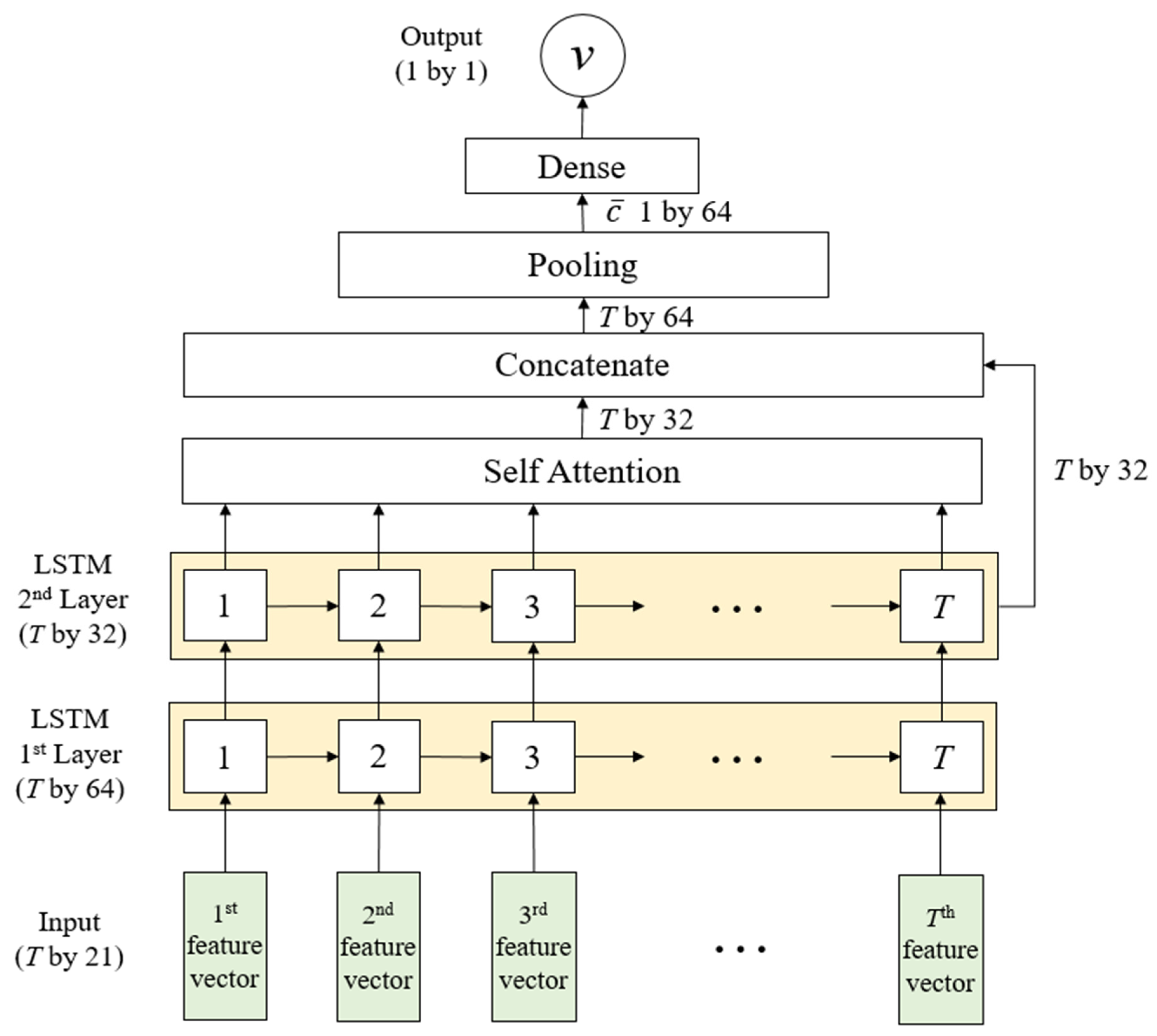
Figure 1. Overall architecture of the proposed model, which combines stacked LSTM layers with a self-attention mechanism to estimate speed from sequential sensor data.
Applsci 15 08824 g001
Figure 2. Experimental setup. (a) Four smartphones (Test phones 1–4) were mounted on the dashboard with different orientations to collect sensor data. (b) An OBD2 device was connected to record reference speed during the experiment.
Applsci 15 08824 g002
Figure 3. Experimental driving trajectories. Red dots mark the starting points, and red arrows indicate the initial driving direction. (a) First scenario: Counterclockwise driving along a rectangular path. (b) Second scenario: Similar counterclockwise path with slight variation. (c) Third scenario: Repetitive turning maneuvers along a looped path.
Applsci 15 08824 g003
Figure 4. Ground truth vehicle velocity obtained from the OBD2 device for each scenario. (a) First scenario. (b) Second scenario. (c) Third scenario.
Applsci 15 08824 g004
Figure 5. Probability density functions of error (m/s) using all with a fixed sequence length of 200. (a) First scenario. (b) Second scenario. (c) Third scenario.
Applsci 15 08824 g005
Figure 6. Cumulative Distribution Function (CDF) of absolute mean error (m/s) for vehicle speed estimation using all features (raw + statistical) with a fixed sequence length of 200. (a) First scenario. (b) Second scenario. (c) Third scenario.
Applsci 15 08824 g006
Figure 7. Comparison between actual vehicle speed from OBD2 and predicted speed using the proposed model under first scenario, with all features (raw + statistical) and the smartphone placed at pitch 90° orientation.
Applsci 15 08824 g007
Table 1. Comparison of deep learning-based inertial navigation models for vehicle positioning.
ReferenceLearning ModelUsed SensorOutputTestbedAccuracy
[30]DNN + LSTMaccelerometer
gyroscope
SpeedUrban and highwayMAE: 0.5 m/s
[31]TCNaccelerometer
gyroscope
TrajectoryUrbanRMSE: 3.2 m
[32]LSTM (DeepVIP-L)
LSTM (DeepVIP-M)
accelerometer
gyroscope
magnetometer
gravity sensor
Speed and headingIndoor parking lotRMSE: 2.5 m
[33]TCNaccelerometer
gyroscope
TrajectoryUrbanRMSE: 2.8 m
Table 2. Model performance evaluation of MAE with all features.
FeatureTScenarioTP1TP2TP3TP4
MAE (m/s)MAE (m/s)MAE (m/s)MAE (m/s)
Raw200First0.230.290.370.31
Second0.210.260.360.24
Third0.280.240.560.30
Statistical200First0.240.400.390.44
Second0.280.310.400.36
Third0.280.290.570.34
Raw + Statistical 200First0.190.290.370.24
Second0.190.240.400.23
Third0.210.210.500.30
Table 3. Model performance evaluation of RMSE with all features.
FeatureTScenarioTP1TP2TP3TP4
RMSE (m/s)RMSE (m/s)RMSE (m/s)RMSE (m/s)
Raw200First0.320.400.490.42
Second0.400.350.470.34
Third0.380.310.690.38
Statistical200First0.340.570.560.70
Second0.430.470.500.50
Third0.400.440.710.45
Raw + Statistical 200First0.280.410.490.31
Second0.300.340.490.34
Third0.300.290.630.40
Table 4. Comparison of estimation accuracy between existing approaches and proposed model.
KF [38]DNN [30]Proposed
RMSE(m/s)0.530.50.38
Disclaimer/Publisher’s Note: The statements, opinions and data contained in all publications are solely those of the individual author(s) and contributor(s) and not of MDPI and/or the editor(s). MDPI and/or the editor(s) disclaim responsibility for any injury to people or property resulting from any ideas, methods, instructions or products referred to in the content.