Abstract
The main anthropogenic sources of air pollution in big cities are vehicular traffic and industrial activities. The emissions of primary pollutants are produced directly from the combustion of fossil fuels of vehicles and industry, whilst the secondary pollutants, such as tropospheric ozone (), are produced from precursors like Carbon monoxide (), among others, and meteorological factors such as radiation. In this study, we analyze the time series of and concentrations monitored by the RAMA program between 2019 and 2023 in the southwest of the Mexico City Metropolitan Area, encompassing the COVID-19 lockdown period declared from March to September–October 2020. After removing cyclic patterns and normalizing the data, we applied informational and topological methods to investigate variability changes in the concentration time series, particularly in response to the lockdown. Following the onset of lockdown measures in March 2020—which led to a significant reduction in industrial activity and vehicular traffic—the informational quantities and Fisher Information Measure (FIM) for revealed significant shifts during the lockdown, while these metrics remained stable for . Also, the coefficient of variation of the degree , which was defined for the network constructed for each series by the Visibility Graph, showed marked changes for but not for . The combined informational and topological analysis highlighted distinct underlying structures: exhibited localized, intermittent emission patterns leading to greater structural complexity, while displayed smoother, less organized variability. Also, the temporal variation of the FIM and provides a means to monitor the evolving statistical behavior of the and time series over time. Finally, the Visibility Graph (VG) method shows a behavioral trend similar to that shown by the informational quantifiers, revealing a significant change during the lockdown for , although remaining almost stable for .
1. Introduction
Air pollution remains a critical challenge in large urban agglomerations due to its complex causes and wide-ranging effects on human health, ecosystems, and climate systems [1]. Among the major pollutants, tropospheric ozone () and carbon monoxide () are particularly relevant in urban areas because of their strong links to anthropogenic emissions, primarily from fossil fuel combustion in the transport and industrial sectors. In cities such as the Mexico City Metropolitan Area (MCMA)—one of the largest urban zones globally with more than 20 million inhabitants—air pollution is driven by high vehicular density (over 5 million vehicles), industrial activities, and unfavorable topography that traps pollutants within a basin-like valley [2,3,4]. is a primary pollutant emitted directly from incomplete combustion processes, especially from gasoline-powered engines, industrial machinery, and residential sources such as gas heaters and stoves [5]. In contrast, tropospheric ozone is a secondary pollutant formed by complex photochemical reactions involving precursors like CO, nitrogen oxides (), volatile organic compounds (), and solar radiation [6,7].
Long-term monitoring data from the Environmental Monitoring Office (DMA-CDMX for its Spanish acronym) [8] indicate that from 2019 to 2023, daily concentrations in the MCMA ranged between 0.6 and 1.2 ppm, with occasional exceedances in traffic-congested zones. Meanwhile, concentrations routinely surpassed the WHO guideline of 70 ppb, particularly in spring months during the afternoon, driven by high solar radiation and stagnant meteorological conditions [2,3,9]. These local trends mirror observations in other urban centers. For instance, cities like Beijing [10] and Delhi [11] have reported similar patterns, where emissions are largely attributed to vehicular traffic, while formation depends heavily on the interaction between and under specific photochemical regimes. Notably, in VOC-limited environments, reducing emissions can paradoxically lead to increased concentrations—an effect observed during the COVID-19 lockdowns in many cities worldwide, including the MCMA. Despite a sharp decrease in and emissions during this period, levels remained stable or even increased due to altered atmospheric chemistry and reduced NO titration [12,13,14].
Such anomalies underscore the need for more advanced analytical tools capable of characterizing the temporal dynamics and inherent complexity of air pollution time series, beyond what traditional statistical methods can capture. Time series of atmospheric pollutant concentrations are, by nature, stochastic processes that may exhibit self-similarity and scale-invariant behaviors across different time scales. In many natural systems, such complex signals often follow a multifractal structure characterized by scaling exponents that vary with scale. Several studies have focused on as a primary pollutant, employing multifractal analysis [15,16] and wavelet-based techniques [13,17,18] to examine temporal dynamics.
While these approaches have yielded valuable insights, they present limitations when it comes to fully capturing the evolving complexity and structural patterns in pollutant behavior. To address these analytical gaps, the present study introduces two complementary methods: the Fisher–Shannon information framework [19,20,21] and the Visibility Graph (VG) method [22,23,24]. These techniques, though widely applied in other disciplines, remain largely underutilized in the analysis of atmospheric pollution time series. Their application offers a novel perspective to uncover hidden patterns, quantify degrees of disorder, and understand the structural evolution of pollutant concentrations.
The Fisher–Shannon method has proven effective in various domains, including geosciences [19] and heavy metal dynamics [25]. Notably, a study in Switzerland used this framework to analyze hourly time series of , , and , revealing a clear relationship between pollutant concentration disorder and the spatial characteristics of monitoring stations—insightful for distinguishing land-use types and human activity patterns [26].
In parallel, the Visibility Graph method has gained attention as a powerful tool for mapping time series into complex networks. By leveraging the topological features of these networks, VG analysis allows for the extraction of meaningful structural information about the dynamics of the original signal. Applications span diverse fields: from seismic activity analysis [27,28] and sea surface temperature fluctuations during El Niño events [29], to the study of dynamics in Guadeloupe [30] and the differentiation of urban vs. rural ozone behaviors [31].
To better understand these dynamics, the present study applies both the Fisher–Shannon and Visibility Graph methods to and time series in the MCMA from 2019 to 2023, including the COVID-19 lockdown period. These tools allow us to identify temporal patterns, assess the degree of disorder in pollutant concentrations, and provide insight into how human activity and meteorological variability influence the atmospheric behavior of key pollutants. By comparing findings within the MCMA and contextualizing them with patterns from other urban regions, this study contributes to a broader understanding of pollution dynamics in complex urban environments.
Although there is a substantial body of research in Mexico focusing on air pollutants—including their concentrations, health impacts, and source attribution, no study to date has applied informational or topological approaches such as the Fisher–Shannon or Visibility Graph methods to explore the underlying dynamical complexity of air pollution time series. This study addresses that gap and proposes a novel methodological perspective to analyze urban air quality in the Mexican context.
2. Materials
Dataset
In Figure 1, the monitoring network is shown; it consists of 34 remote stations located MCMA and driven by the Automatic Environmental Monitoring Network program (Red Automatica de Monitoreo Ambiental (RAMA)).
Our study examines the temporal dynamics of CO and concentrations, measured at seven monitoring stations (currently in operation and measuring the desired parameters, see Figure 1) located in the southwestern zone of MCMA, which is characterized by the highest levels of and . The selection of this zone as the focus of analysis is based on its high vulnerability to the accumulation of atmospheric pollutants, resulting from a combination of meteorological, geographic, and urban factors. According to the Mexico City Secretariat of the Environment [8], in 2022, a predominant north-to-south wind pattern was observed—consistent with previous years—especially from April to November, which facilitates the transport of pollutants toward the southwest. In the remaining months, wind behavior was more variable, with east–northeast and southeasterly flows converging toward the center, creating zones of confluence that further exacerbate pollutant accumulation. These circulation patterns are compounded by local atmospheric conditions, such as intense solar radiation, high afternoon temperatures, and low cloud cover, which enhance the photochemical formation of ozone. Additionally, the basin’s topography—surrounded by mountain ranges—acts as a natural barrier, limiting the dispersion of pollutants and promoting their concentration in this sector. According to the National Air Quality Report [32], the southwestern zone consistently records the highest concentrations of ozone in Mexico City, particularly during the spring months. These conditions, combined with the continuous influx of emissions from vehicular and domestic sources, justify the selection of this region as a critical area to evaluate the spatiotemporal behavior of and in the present study.

Figure 1.
Spatial distribution of all monitoring stations within the MCMA. The bold contour indicates the boundary of Mexico City. The southwest zone is conformed by the stations highlighted with red stars [33].
The sampling time is 1 h. Figure 2 shows the time variation of the two pollutants studied. Each hourly value is the spatial average among the stations (See section “Data Availability Statement”). Outliers caused by instrument failures or human errors are eliminated; the single gaps are filled by the mean of the nonzero neighboring values, while longer gaps are filled by using the procedure developed by [34]. The percentage of data missing is less than 0.1%.
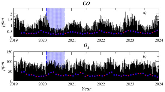
Figure 2.
The two time series analyzed: (a) and (b) . Also, the yearly average concentrations of the three pollutants are represented as dots. The shaded area represents the pandemic lockdown.
At the end of 2020, an increase in air pollutant emissions in MCMA was observed associated with a gradual return to mobility after lifting some of the preventive measures implemented during the COVID-19 pandemic. This increase was related to the reactivation of economic activities, according to the Local Mobility Reports [35], the increase in vehicular traffic, and the more significant influx of people into public spaces, highlighting the impact of urban mobility on air quality in the region. According to the Environmental Monitoring Office (Dirección de Monitoreo Atmosférico in Mexico City, DMA-CDMX), the highest levels are associated with the so-called ozone season, which occurs from February to June. When meteorological conditions favor warm weather and intense solar radiation, the atmosphere’s photochemical activity increases, favoring the formation of ozone. In addition, when a high pressure system is present, the pollutant stagnates, and, as a result, its concentrations increase (https://www.google.com/covid19/mobility/, accessed on 5 August 2025).
3. Methods
3.1. The Fisher–Shannon Method
To quantify the local and global smoothness of the distribution of analyzed time series, Fisher Information Measure (FIM) and the Shannon entropy (SE) are applied, which are defined as follows:
where is the distribution of the series x. However, it most commonly uses the Shannon entropy power (SEP), , instead of SE, which is positively defined:
FIM and are not independent of each other due to the isoperimetric inequality:
where the spatial dimension is for time series. The accurate estimation of is fundamental to obtain reliable values of informational quantities. For calculating FIM and , we applied the kernel-based approach because it is better than the discrete-based approach in estimating the probability density function [36]. Thus, applying this method, is given by the following formula:
where M and b denote the length of the series and the bandwidth, respectively, while is the kernel, a continuous, symmetric, and non-negative function satisfying the following two constraints:
is estimated by means of an optimized integrated procedure using the algorithms of Troudi et al. [37] and Raykar and Duraiswami [38] with the Gaussian kernel:
3.2. The Visibility Graph Analysis
The Visibility Graph (VG) [39] is a method that transforms a time series in a graph or network. The nodes are given by the values of the series, and the links between them satisfy the following geometrical visibility rule:
where . In practice, two values, and , are visible to each other if any other value satisfies Equation (1).
The mathematical representation of the graph is given by the adjacency matrix , which is defined as follows:
Equation (2) is a used to describe the connections between nodes in a graph and provides a way to encode the visibility relationships between values in a time series, indicating which values are directly visible to each other based on the visibility criterion (Equation (1)).
The degree , defined in Equation (3), represents the number of links departing from the node i to any other node of the network. It is one of the parameters used to describe the network derived from the visibility graph.
4. Data Analysis
In Figure 2, the raw data of two gases analyzed are shown. The frequency peaks at 24 h, 12 h, and 8 h, clearly visible in the power spectra, suggest that the temporal fluctuations of the three pollutants are modulated by meteo-climatic cycles (Figure 3). The presence of seasonal components in the time series of CO and O3 has been reported by [15] in other cities.
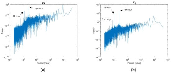
Figure 3.
Power spectrum of the original hourly time series of (a) and (b) .
Before applying the Fisher–Shannon and the Visibility Graph analyses, we removed the cyclic patterns from the time series by applying the following procedure:
where
- is the original hourly value at time t;
- is the mean of the hourly values calculated for the same hour h, day d, and month m across different years;
- is the standard deviation calculated for the same hour h, day d, and month m across different years;
- is the resulting normalized value.
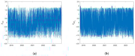
Figure 4.
Normalized hourly time series of (a) and (b) .
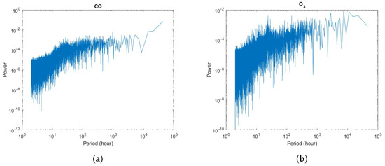
Figure 5.
Power spectrum of the detrended hourly time series of (a) and (b) .
We applied the FS analysis to the normalized series. The two series are characterized by almost identical values of (0.68–0.69) but very different values of FIM (3.65 and 9.68) (Table 1). If the degree of disorder is practically the same for the two series, the degree of organization is the highest for and lowest for . Looking at the density of the two normalized series (Figure 6), is characterized by multiple peaks that may contribute to the larger FIM.

Table 1.
Informational and topological parameters for the analyzed normalized series.
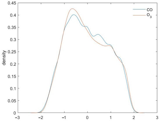
Figure 6.
Distribution of the normalized time series of and .
By converting the time series into graphs using the VG method, we calculated the temporal variation of the degree for each series (Figure 7). The degree of a value reflects its capability to be a hub of the series; thus, the larger the degree of a value, the larger its capability to “attract” the other values of the series. Table 1 shows, for the two normalized series, the mean degree , the standard deviation , and the coefficient of variation of the degree, defined as follows:
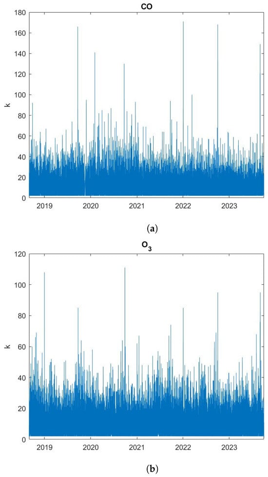
Figure 7.
Time distribution of the degree k of (a) and (b) .
For , all the three parameters are slighlty larger than the corresponding values for , indicating that is characterized by more hubs than . This further suggests a greater complexity in the network generated by the VG for compared to , due to the presence of links between values that may be located far apart from each other, if one of them is a hub. The larger and of could also indicate a greater complexity of compared to regarding a more extensive network heterogeneity.
To identify potential patterns related to the COVID-19 lockdown, we analyzed the temporal variations in (Figure 8a), FIM (Figure 8b), and the coefficient of variation in the degree of the network constructed from the time series using the VG method (Figure 8c). By shifting a 6-month time window over the series in 5-day steps, we calculated these three parameters within each moving window, associating the resulting values with the ending time of the window. This choice balances the need for statistical robustness with the ability to resolve temporal changes in the series. Each 6-month window contains approximately 4,320 data points, ensuring a sufficiently large sample size for reliable estimation of the probability density function, on which the FS method is based, and for the calculation of the coefficient of variation of the degree of the visibility network. A larger dataset within each window leads to a more accurate characterization of the signal’s statistical features. Moreover, the 6-month length allows for an adequate number of windows to be positioned before the onset of the COVID-19 pandemic, making it possible to observe and compare the behavior of the FS and VG complexity in both the pre-COVID and COVID-affected periods. Using substantially longer windows would have reduced the resolution in the pre-COVID phase, hindering the detection of the changes that emerged during the pandemic.
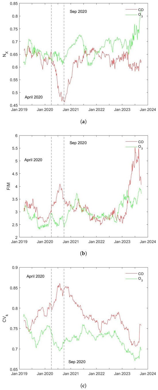
Figure 8.
Time variation in (a) , (b) FIM, and (c) .
In all cases, we observe that during the COVID-19 lockdown, approximately between April and September 2020, the three parameters show a clear difference between and . In particular, for , decreases, while FIM and increase. During lockdown, the three parameters for remain almost stationary and do not exhibit any significant anomalous trends. After lockdown, the three parameters for and tend to align with each other, indicating a clear correlation. The combined FS and VG analyses reveal that the temporal behavior of CO is shaped by more localized and intermittent emissions, leading to high structural complexity and organization. , by contrast, reflects broader-scale chemical processes and environmental modulation, resulting in smoother, less structured variability. These insights help to bridge the gap between pollutant emission mechanisms and their statistical representation, offering a valuable perspective for interpreting air quality time series.
While the combined use of the FS and VG methods has enabled us to uncover complex patterns and meaningful structural differences between and , it is important to acknowledge certain inherent limitations of the analysis. The use of a 6-month moving window provided a good balance between statistical robustness and temporal resolution; however, this approach may smooth out very short-term events or abrupt changes. Additionally, although the visibility graph technique effectively captures structural properties of time series, it can be sensitive to outliers or noise, potentially affecting metrics such as hub identification or degree heterogeneity. On the other hand, while the data used are of high quality and resolution, they may not fully reflect the spatial variability of emission sources or local meteorological influences. Finally, although a clear signal was identified during the COVID-19 lockdown period, it is possible that other concurrent factors—such as seasonal effects or regional atmospheric processes—also contributed to the observed patterns. Nevertheless, the results provide a solid foundation for advancing the understanding of the temporal dynamics of urban pollutants and exploring new approaches for air quality time series analysis.
5. Conclusions
This study applied two complementary analytical approaches—the Fisher–Shannon information framework and the Visibility Graph method—to analyze the time series of and concentrations in the southwest of the MCMA from 2019 to 2023, including during the COVID-19 lockdown. Our results provide clear evidence of differential responses between primary and secondary pollutants. The informational metrics NX and FIM detected a substantial shift in the statistical behavior of during the lockdown period. These changes reflect the abrupt reduction in vehicular activity and industrial emissions and reveal a decrease in complexity and disorder consistent with a more homogeneous and less volatile emission profile during that time. Conversely, the stability of and FIM values for suggests that this secondary pollutant is governed by slower, large-scale chemical and meteorological processes that are less immediately responsive to localized emission reductions. The VG method offered a topological perspective on these findings. The coefficient of variation of the node degree in the constructed networks showed changes in time series complexity similar to those detected by the Fisher–Shannon metrics. For , the VG structure remained relatively stable, supporting the conclusion that its variability is less sensitive to short-term anthropogenic shifts and is instead modulated by regional photochemistry, precursor ratios, and seasonal solar radiation patterns. These findings have important practical and methodological implications. They confirm the usefulness of as a near-real-time indicator of changes in urban activity while highlighting the complex, nonlinear nature of formation and the need for integrated mitigation strategies that consider precursor dynamics and meteorological conditions. The informational and topological methods applied here can detect subtle changes in pollutant behavior, offering valuable diagnostic insights that complement traditional air quality assessments. Their scalability and adaptability make them suitable for application in other urban contexts, and they hold potential as early-warning tools for identifying anomalous pollution patterns linked to extreme events or policy shifts. The integration of informational theory and complex network analysis provides a powerful framework to explore the dynamics of air pollutant behavior. In contexts like MCMA, where emissions are intense and meteorological constraints severe, such approaches offer a more nuanced and mechanistic understanding of pollutant variability—one that is essential for designing robust, adaptive, and evidence-based air quality policies.
Author Contributions
Conceptualization, A.R.-R., P.R.C.-M., I.R.-R., M.L. and L.T.; Methodology, A.R.-R., P.R.C.-M., I.R.-R., M.L. and L.T.; Software, A.R.-R., I.R.-R., M.L. and L.T.; Validation, A.R.-R., P.R.C.-M., I.R.-R., M.L. and L.T.; Investigation, A.R.-R., P.R.C.-M., I.R.-R., M.L. and L.T.; Data curation, A.R.-R., P.R.C.-M., I.R.-R., M.L. and L.T.; Writing—original draft, A.R.-R., P.R.C.-M., I.R.-R., M.L. and L.T. All authors have read and agreed to the published version of the manuscript.
Funding
This research received no external funding.
Data Availability Statement
The instructions to download the dataset are available on the website: http://www.aire.cdmx.gob.mx/default.php, accessed on 5 August 2025.
Acknowledgments
A.R.R. and P.R.C.-M. thank to Basic Science Department of UAM Azcapotzalco-México. I.R.-R. thanks to COFAA and EDI IPN-México. L.T. and M.L. thank to CNR-Italy. The authors also acknowledge to SECIHTI-México.
Conflicts of Interest
The authors declare no conflicts of interest.
References
- World-Health-Organization. Health Aspects of Air Pollution with Particulate Matter, Ozone and Nitrogen Dioxide: Report on a WHO Working Group, Bonn, Germany 13–15 January 2003; Technical Report; WHO Regional Office for Europe: Copenhagen, Denmark, 2003. [Google Scholar]
- Molina, L.T.; Madronich, S.; Gaffney, J.; Apel, E.; de Foy, B.; Fast, J.; Ferrare, R.; Herndon, S.; Jimenez, J.L.; Lamb, B.; et al. An overview of the MILAGRO 2006 Campaign: Mexico City emissions and their transport and transformation. Atmos. Chem. Phys. 2010, 10, 8697–8760. [Google Scholar] [CrossRef]
- Garzón, J.P.; Huertas, J.I.; Magaña, M.; Huertas, M.E.; Cárdenas, B.; Watanabe, T.; Maeda, T.; Wakamatsu, S.; Blanco, S. Volatile organic compounds in the atmosphere of Mexico City. Atmos. Environ. 2015, 119, 415–429. [Google Scholar] [CrossRef]
- Cassiani, M.; Stohl, A.; Eckhardt, S. The dispersion characteristics of air pollution from the world’s megacities. Atmos. Chem. Phys. 2013, 13, 9975–9996. [Google Scholar] [CrossRef]
- Secretaría de Salud. NORMA Oficial Mexicana NOM-021-SSA1-2021, Salud ambiental. Criterio para evaluar la calidad del aire ambiente, con respecto al monóxido de carbono (CO). Valores normados para la concentración de monóxido de carbono (CO) en el aire ambiente, como medida de protección a la salud de la población. Diario Oficial de la Federación, 1 November 2021; 1–6. [Google Scholar]
- Monks, P.S.; Archibald, A.; Colette, A.; Cooper, O.; Coyle, M.; Derwent, R.; Fowler, D.; Granier, C.; Law, K.S.; Mills, G.; et al. Tropospheric ozone and its precursors from the urban to the global scale from air quality to short-lived climate forcer. Atmos. Chem. Phys. 2015, 15, 8889–8973. [Google Scholar]
- Akimoto, H. Global air quality and pollution. Science 2003, 302, 1716–1719. [Google Scholar] [CrossRef] [PubMed]
- Secretaría del Medio Ambiente de la Ciudad de México, Dirección de Monitoreo de Calidad del Aire. Calidad del aire en la Ciudad de México, Informe 2022. 2024. Available online: http://www.aire.cdmx.gob.mx/default.php (accessed on 8 July 2025).
- Baklanov, A.; Molina, L.T.; Gauss, M. Megacities, air quality and climate. Atmos. Environ. 2016, 126, 235–249. [Google Scholar] [CrossRef]
- Zhang, K.; Liu, Z.; Zhang, X.; Li, Q.; Jensen, A.; Tan, W.; Huang, L.; Wang, Y.; de Gouw, J.; Li, L. Insights into the significant increase in ozone during COVID-19 in a typical urban city of China. Atmos. Chem. Phys. 2022, 22, 4853–4866. [Google Scholar] [CrossRef]
- Rathod, A.; Sahu, S.; Singh, S.; Beig, G. Anomalous behaviour of ozone under COVID-19 and explicit diagnosis of O3-NOx-VOCs mechanism. Heliyon 2021, 7, e06142. [Google Scholar] [CrossRef] [PubMed]
- Wałaszek, K.; Kryza, M.; Werner, M. The role of precursor emissions on ground level ozone concentration during summer season in Poland. J. Atmos. Chem. 2018, 75, 181–204. [Google Scholar] [CrossRef]
- Aguilar-Velázquez, D.; Reyes-Ramírez, I. A wavelet analysis of multiday extreme ozone and its precursors in Mexico city during 2015–2016. Atmos. Environ. 2018, 188, 112–119. [Google Scholar] [CrossRef]
- Wang, Y.; Guo, H.; Zou, S.; Lyu, X.; Ling, Z.; Cheng, H.; Zeren, Y. Surface O3 photochemistry over the South China Sea: Application of a near-explicit chemical mechanism box model. Environ. Pollut. 2018, 234, 155–166. [Google Scholar] [CrossRef]
- Pavón-Domínguez, P.; Plocoste, T. Coupled multifractal methods to reveal changes in nitrogen dioxide and tropospheric ozone concentrations during the COVID-19 lockdown. Atmos. Res. 2021, 261, 105755. [Google Scholar] [CrossRef]
- Lee, C.K. Multifractal characteristics in air pollutant concentration time series. Water Air Soil Pollut. 2002, 135, 389–409. [Google Scholar] [CrossRef]
- Nikolopoulos, D.; Moustris, K.; Petraki, E.; Koulougliotis, D.; Cantzos, D. Fractal and long-memory traces in PM10 time series in Athens, Greece. Environments 2019, 6, 29. [Google Scholar] [CrossRef]
- Chen, Y.; Shi, R.; Shu, S.; Gao, W. Ensemble and enhanced PM10 concentration forecast model based on stepwise regression and wavelet analysis. Atmos. Environ. 2013, 74, 346–359. [Google Scholar] [CrossRef]
- Guignard, F.; Laib, M.; Amato, F.; Kanevski, M. Advanced analysis of temporal data using Fisher-Shannon information: Theoretical development and application in geosciences. Front. Earth Sci. 2020, 8, 255. [Google Scholar] [CrossRef]
- Martin, M.; Pennini, F.; Plastino, A. Fisher’s information and the analysis of complex signals. Phys. Lett. A 1999, 256, 173–180. [Google Scholar] [CrossRef]
- Martin, M.; Perez, J.; Plastino, A. Fisher information and nonlinear dynamics. Phys. A Stat. Mech. Its Appl. 2001, 291, 523–532. [Google Scholar] [CrossRef]
- Gómez-Gómez, J.; Carmona-Cabezas, R.; Sánchez-López, E.; Gutierrez de Rave, E.; Jiménez-Hornero, F.J. Analysis of air mean temperature anomalies by using horizontal visibility graphs. Entropy 2021, 23, 207. [Google Scholar] [CrossRef] [PubMed]
- Carmona-Cabezas, R.; Ariza-Villaverde, A.B.; de Ravé, E.G.; Jiménez-Hornero, F.J. Visibility graphs of ground-level ozone time series: A multifractal analysis. Sci. Total Environ. 2019, 661, 138–147. [Google Scholar] [CrossRef]
- Carmona-Cabezas, R.; Gómez-Gómez, J.; Ariza-Villaverde, A.B.; de Ravé, E.G.; Jiménez-Hornero, F.J. Can complex networks describe the urban and rural tropospheric O3 dynamics? Chemosphere 2019, 230, 59–66. [Google Scholar] [CrossRef] [PubMed]
- Telesca, L.; Caggiano, R.; Lapenna, V.; Lovallo, M.; Trippetta, S.; Macchiato, M. Analysis of dynamics in Cd, Fe, and Pb in particulate matter by using the Fisher–Shannon method. Water Air Soil Pollut. 2009, 201, 33–41. [Google Scholar] [CrossRef]
- Amato, F.; Laib, M.; Guignard, F.; Kanevski, M. Analysis of air pollution time series using complexity-invariant distance and information measures. Phys. A Stat. Mech. Its Appl. 2020, 547, 124391. [Google Scholar] [CrossRef]
- Telesca, L.; Lovallo, M. Analysis of seismic sequences by using the method of visibility graph. Europhys. Lett. 2012, 97, 50002. [Google Scholar] [CrossRef]
- Ramírez-Rojas, A.; Flores-Márquez, E.L.; Vargas, C.A. Visibility Graph Analysis of the Seismic Activity of Three Areas of the Cocos Plate Mexican Subduction Where the Last Three Large Earthquakes (M> 7) Occurred in 2017 and 2022. Entropy 2023, 25, 799. [Google Scholar] [CrossRef] [PubMed]
- Telesca, L.; Lovallo, M.; Pierini, J.O. Visibility graph approach to the analysis of ocean tidal records. Chaos Solit. Fractals 2012, 45, 1087–1091. [Google Scholar] [CrossRef]
- Pierini, J.O.; Lovallo, M.; Telesca, L. Visibility graph analysis of wind speed records measured in central Argentina. Phys. A 2012, 391, 5041–5048. [Google Scholar] [CrossRef]
- Kernighan, B.W.; Lin, S. An efficient heuristic procedure for partitioning graphs. Bell Syst. Tech. J. 1970, 49, 291–307. [Google Scholar] [CrossRef]
- Instituto Nacional de Ecología y Cambio Climático. Informe Nacional de Calidad del Aire 2022. 2025. Available online: https://sinaica.inecc.gob.mx/archivo/informes/Informe2022.pdf (accessed on 8 July 2025).
- Secretaría del Medio Ambiente de la Ciudad de México, Dirección de Monitoreo de Calidad del Aire. Caracterización, Evaluación y Análisis del Entorno Físico y de la Representatividad en las Estaciones del Sistema de Monitoreo Atmosférico de la Ciudad de México. 2021. Available online: http://www.aire.cdmx.gob.mx/descargas/publicaciones/simat-entornos.pdf (accessed on 15 April 2025).
- Diosdado, A.M.; Coyt, G.G.; López, J.B.; del Rio Correa, J. Multifractal analysis of air pollutants time series. Rev. Mex. Física 2013, 59, 7–13. [Google Scholar]
- De La Cruz-Hernández, S.I.; Álvarez Contreras, A.K. COVID-19 Pandemic in Mexico: The Response and Reopening. Disaster Med. Public Health Prep. 2022, 16, 2264–2266. [Google Scholar] [CrossRef]
- Telesca, L.; Lovallo, M. On the performance of Fisher Information Measure and Shannon entropy estimators. Phys. A Stat. Mech. Its Appl. 2017, 484, 569–576. [Google Scholar] [CrossRef]
- Troudi, M.; Alimi, A.; Saoudi, S. Analytical plug-in method for kernel density estimator applied to genetic neutrality study. EURASIP J. Adv. Signal Process. 2008, 2008, 739082. [Google Scholar] [CrossRef]
- Raykar, V.; Duraiswami, R. Fast optimal bandwidth selection for kernel density estimation. In Proceedings of the 2006 SIAM International Conference on Data Mining; SIAM: Philadelphia, PA, USA, 2006; pp. 524–528. [Google Scholar]
- Lacasa, L.; Luque, B.; Ballesteros, F.; Luque, J.; Nuno, J.C. From time series to complex networks: The visibility graph. Proc. Natl. Acad. Sci. USA 2008, 105, 4972–4975. [Google Scholar] [CrossRef] [PubMed]
Disclaimer/Publisher’s Note: The statements, opinions and data contained in all publications are solely those of the individual author(s) and contributor(s) and not of MDPI and/or the editor(s). MDPI and/or the editor(s) disclaim responsibility for any injury to people or property resulting from any ideas, methods, instructions or products referred to in the content. |
© 2025 by the authors. Licensee MDPI, Basel, Switzerland. This article is an open access article distributed under the terms and conditions of the Creative Commons Attribution (CC BY) license (https://creativecommons.org/licenses/by/4.0/).