Predicting Relative Density of Pure Magnesium Parts Produced by Laser Powder Bed Fusion Using XGBoost

Featured Application

The optimized LPBF process with XGBoost modelling predicts magnesium component density, improving manufacturing efficiency for potential lightweight and high-strength parts in aerospace, automotive and biomedical applications.

Abstract

In this work, Laser Powder Bed Fusion (LPBF), an additive manufacturing (AM) process, was optimised to produce pure magnesium components. The focus of the presented work is on the prediction of the relative product density using the machine learning model XGBoost to improve the production process and thus the usability of the material for practical use. Experimental tests with different parameters, laser power, scanning speed and layer thickness, and fixed parameters, track overlapping and hatching distance, were analysed and resulted in relative material densities between 89.29% and 99.975%. The XGBoost model showed high predictive power, achieving an R² test result of 0.835, a mean absolute error (MAE) of 0.728 and a root mean square error (RMSE) of 0.982. Feature importance analysis showed that the interaction of laser power and scanning speed had the largest influence on the predictions at 35.9%, followed by laser power × layer thickness at 29.0%. The individual contributions were laser power (11.8%), scanning speed (10.7%), scanning speed × layer thickness (9.0%) and layer thickness (3.6%). These results provide a data-based method for LPBF parameter settings that improve manufacturing efficiency and component performance in the aerospace, automotive and biomedical industries and identify optimal parameter regions for a high density, serving as a pre-optimisation stage.

1. Introduction

Laser Powder Bed Fusion (LPBF) is a widely used additive manufacturing (AM) process for the production of complex metal parts that require high precision [1]. Magnesium (Mg) and its alloys are increasingly used in AM, especially in LPBF [2,3], due to their exceptionally lightweight properties and high strength-to-weight ratio, qualities highly sought after in aerospace [4], automotive [5] and biomedical applications [6,7].

However, the LPBF process for Mg poses a challenge for production, mainly due to the material’s high reactivity and tendency to oxidise [8]. During the LPBF process, the low ignition temperature [9] and its high affinity for oxygen can lead to the formation of oxide layers, resulting in defects such as porosity, cracks and inclusions that affect the density and mechanical integrity of the manufactured parts, although progress in addressing these problems has been made [10,11].

Achieving high density is crucial to ensure the performance and reliability of the produced parts in certain applications, especially in load-bearing biomedical implants [3] where mechanical strength is critical. In study [12], the authors investigated stochastic pure Mg foam using LPBF. The results of the study showed that when the volumetric energy density was increased from 20 to 40 J mm⁻³, the porosity of the product decreased from 42.7% to 40.5% while its compressive strength increased from 37 MPa to 46 MPa, demonstrating the importance of product density in determining mechanical properties, with lower porosity correlating with higher strength. It is well established that product density plays a major role in the resulting mechanical properties, making density optimisation a priority when working with LPBF made of Mg.

The effects of changing parameters such as laser power, scanning speed, track overlap, hatch spacing and layer thickness have a direct and proven influence on the product [13,14]. Traditional approaches to LPBF process parameter optimisation with the aim of achieving high density involve extensive and iterative experimental trials, which are both time and resource intensive. However, due to the complex relationships between these parameters, e.g., the trade-off between laser power and scanning speed, which influences the energy density, it can be difficult to determine the optimal settings using only traditional approaches. The systematic approach in [15], where the authors optimised the parameters for the LPBF process of low-alloy steel, has shown that the optimisation of the process parameters is necessary to avoid defects such as a lack of fusion and keyholing [16,17,18]. This methodology can also be applicable to Mg given the similarity in process challenges and has been applied to Mg alloys [19].

Machine learning (ML) methods have provided viable solutions by developing predictive models that can efficiently represent the complex relationships between process parameters and part properties, which have reduced the need for extensive experimentation [20,21,22]. In this research, XGBoost [23], a known gradient boosting framework, was selected due to its proven efficiency in handling regression tasks with structured data. The method is able to capture non-linear relationships and provide interpretable insights by analysing the significance of features. In study [24], the effectiveness of XGBoost in predicting the density of Ti-6Al-4V alloy parts produced by selective laser melting (SLM) was demonstrated. The model achieved high accuracy despite a small data set and showed better values for error metrics compared to artificial neural networks and support vector regression models.

In this paper, the data set includes experimental runs using different LPBF parameter settings. By analysing the importance of process features, the results identify and quantify the impact of each parameter on product density, thus providing a data-driven framework to improve the efficiency of the LPBF process in the production of Mg parts. This approach addresses the challenges of traditional optimisation while harnessing the power of ML with the aim of supporting the development of high-density Mg parts suitable for advanced applications. Although previous studies have applied ML to AM, this study focuses specifically on pure magnesium, a reactive and under-researched material in LPBF, and quantitatively demonstrates how parameter interactions dominate density results.

2. Materials and Methods

2.1. Input Variable Intervals

The selected key parameters of the LPBF process in this research were as follows:

• Laser power, which represents the energy output of the laser source during the melting process and affects the ability to effectively fuse powder particles [25].
• Scanning speed, which determines the speed at which the laser beam moves across the powder bed, affecting melting efficiency [26].
• Track overlapping, which indicates the degree of overlap between neighbouring laser scan tracks and affects the uniformity of the melt pool and the structural integrity of the part [27].
• Hatch spacing, the distance between parallel scan lines in the powder bed, which affects the energy distribution and consolidation of the material during layer formation [28].
• Layer thickness, the height of each powder layer deposited during the LPBF process, which affects the resolution, build time and thermal behaviour of the part to be produced [29].

The selected inputs are shown in

Table 1. Process parameters and their intervals.

Parameter	Min Value	Max Value	Status
Laser power [W]	40	150	Variable
Scanning speed [mm/s]	200	1500	Variable
Track overlapping [%]	/	/	Fixed value at 30 %
Hatch spacing [mm]	/	/	Fixed value at 0.035
Layer thickness [mm]	0.025	0.035	Variable

, while the values are listed in

Table A1. Experimental data used for model training and testing.

Data Used for Training
Laser Power [W]	Scanning Speed [mm/s]	Layer Thickness [mm]	Relative Density [%]
120	1200	0.035	99.263
80	800	0.05	96.689
100	1000	0.05	90.929
100	1100	0.035	94.183
85	800	0.05	89.29
200	2000	0.05	94.573
110	1050	0.05	96.829
150	1500	0.035	98.084
90	900	0.05	97.841
70	750	0.05	95.917
150	3000	0.05	90.399
190	2700	0.035	94.737
120	1150	0.05	96.987
95	1000	0.05	98.213
150	2500	0.05	92.211
110	1500	0.035	97.14
85	850	0.05	92.759
175	1750	0.035	97.211
90	900	0.035	93.918
75	750	0.05	96.51
120	1200	0.025	99.975
60	700	0.05	95.43
95	900	0.05	90.027
100	1100	0.05	98.215
200	2500	0.05	92.016
85	850	0.05	97.183
95	950	0.05	89.841
150	1500	0.05	98.469
90	850	0.05	90.29
90	900	0.05	91.363
175	1750	0.05	97.87
95	1000	0.035	93.268
Data Used for Testing
Laser Power [W]	Scanning Speed [mm/s]	Layer Thickness [mm]	Relative Density [%]
110	1100	0.05	97.251
150	2100	0.035	97.125
120	1200	0.05	97.674
55	700	0.05	94.959
200	3000	0.05	91.956
150	2000	0.05	94.428
65	700	0.05	95.952
100	950	0.05	91.283
195	1950	0.05	96.687

for better readability. The parameter intervals were determined regarding the machine capability and work conducted by researchers [3,8].

Certain process parameters such as hatch spacing and track overlapping were kept constant to ensure consistency and minimise the complexity of the experimental design. Overlapping, which was set at 30%, is a calculated parameter that depends on the size of the laser spot and the hatch distance and significantly affects the stability of the melt pool and the density of the parts. Accordingly, the hatch spacing was set to 0.035 mm to ensure uniform energy distribution and reduce discrepancies in the thermal behaviour of the individual layers. By adjusting these parameters, attention could be focussed on the main variables—laser power, scanning speed and layer thickness—allowing a more direct assessment of their different effects on the final quality of the part. This method increased the reliability and clarity of the results by reducing the number of interacting elements.

2.2. Experimental Work

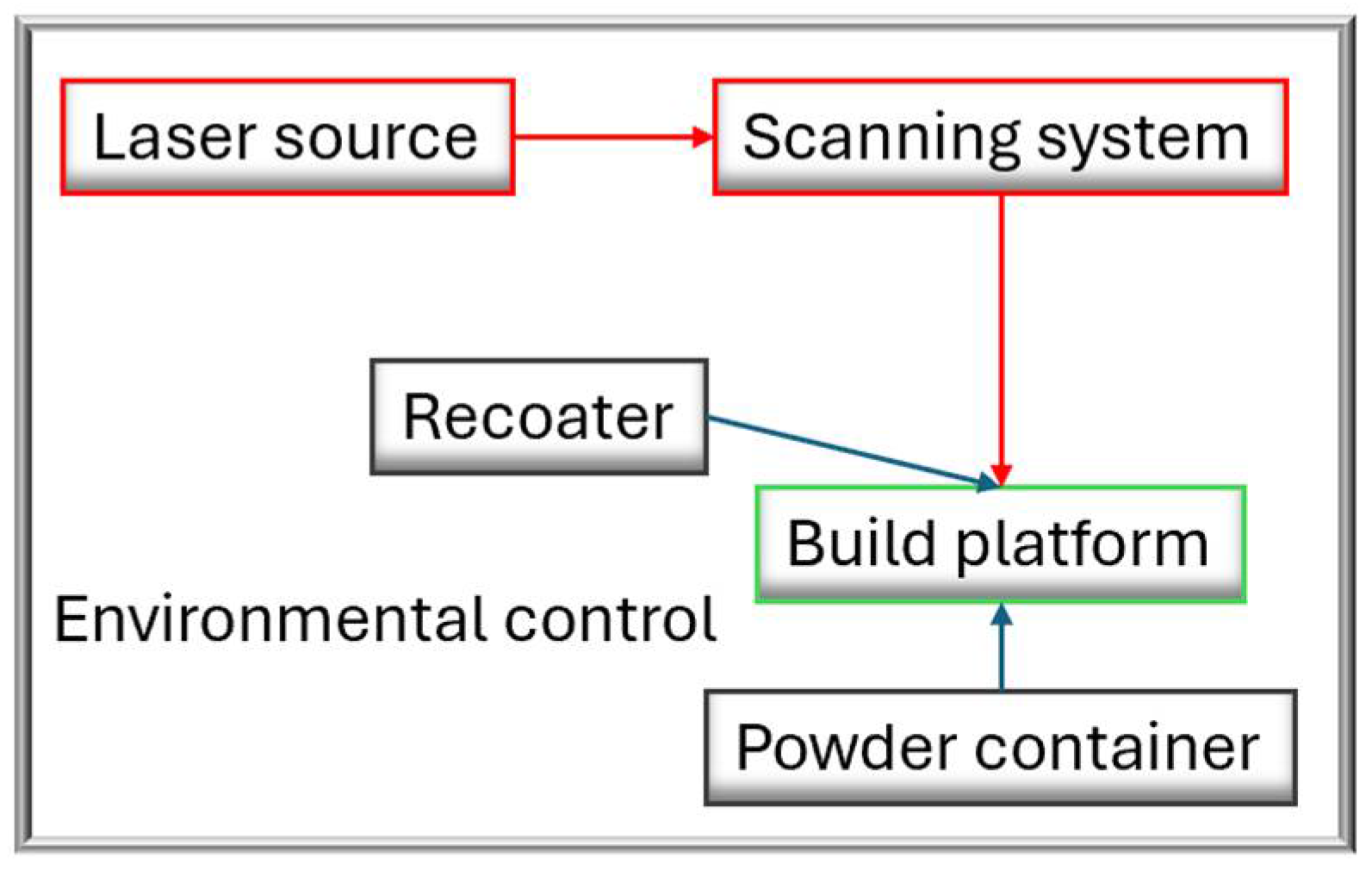
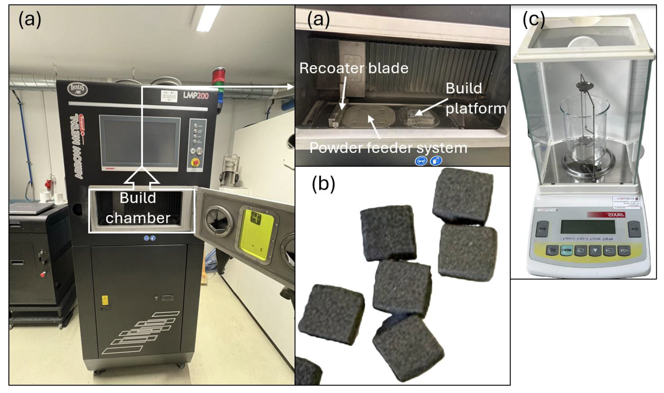
2.2.1. Experimental Setup

Various combinations of laser power, scanning speeds, track overlapping, hatching distances and layer thicknesses were used to determine the melting behaviour and the resulting product density. In addition to the machine runs, the resulting densities were also measured and the next machine runs were followed. While no official design of experiments (DOE), like the Box–Behnken Design (BBD) or Central Composite Design (CCD), was utilised because of limitations in machine time and material resources, the experimental strategy adhered to an organised grid-based method. To ensure adequate coverage and independence within the parameter space, the grid-based experimental design was analysed for parameter distribution and correlations. The configuration varied in laser power (60–200 W), scanning speed (700–3000 mm/s) and layer thickness (0.025–0.05 mm) over 42 trials, ensuring comprehensive coverage with 17 power variations, 19 scanning speeds and 3 layer thicknesses. The correlation matrix showed weak relationships for layer thickness (r = −0.1509 with laser power, r = −0.1134 with scanning speed), but a strong relationship between laser power and scanning speed (r = 0.8814). This combination, which is typical in additive manufacturing to balance the energy input [30], represents a pairing of parameters controlled by the process. The different parameter levels guaranteed a thorough sampling of the parameter space. This guaranteed diverse sampling throughout the established parameter space while preventing unnecessary configurations. Future research will apply formal DOE methods.

2.2.2. Powder Material Properties

Pure magnesium powder (powder composition in

Table 2. Powder composition.

Composition	Percentage by Weight [wt%]
moisture	<0.08
undissolved HCl substance	<0.047
Fe	<0.045
Zn	<0.008
Cl	<0.004
Mg	Balance

) provided by Nanografi Nano Technology, Germany, was used to fabricate the samples. The powder particles were almost spherical and had a diameter between 35 µm and 45 µm. Although the chosen layer thicknesses (0.025–0.035 mm) were smaller than the nominal average particle size of the powder (35–45 µm), they were intentionally chosen to improve the process results. Thinner layers contribute to improved resolution and surface quality while reducing the likelihood of porosity by promoting better melt pool stability and interlayer bonding. In addition, the high energy density and penetration depth that characterise the LPBF process enable effective melting and consolidation, even at layer thicknesses below the average particle size. This strategy enables the production of parts with higher density and finer microstructural properties.

2.2.3. Manufacturing Process

The manufacturing process (schematically presented on Figure 1) was carried out using an LMP200 system (Figure 2a) from Arrow Metal Printing, equipped with a Yb/fibre laser (peak power: 200 W), galvanometer scanner by Raylase and a sealed, inert argon environment to ensure that oxygen levels remained below 10 ppm. This level of environmental control is particularly important when handling pure Mg, a highly reactive substance that is susceptible to oxidation and fire at high temperatures.

The process began with the supply of metal powder from the powder container, which the recoater distributed in a thin layer on the build platform. A laser source emitted a beam that was directed by the scanner system to selectively melt the powder layer according to the design of the sample. Once melted, the build platform lowered and the recoater applied a new layer of powder, repeating the cycle until the sample was complete. The environmental control system maintained an inert atmosphere to prevent oxidation during melting. The carried-out process was typical of LPBF [31].

Each design consisted of cubic samples measuring 6 × 6 × 6 mm³ (Figure 2b), fabricated on 2 mm thick support pillars to improve adhesion to the substrate and minimise deformation caused by residual stresses. The geometry of the support was chosen to ensure thermal stability throughout the process. For each set of parameters, 3 samples were created. Selected combinations of laser power, scanning speed and layer thickness were used in a grid of experimental settings. The selection was based on initial evaluations and established LPBF process parameters for magnesium.

The hatch distance and track overlap remained unchanged for all experiments to focus on the effects of the three main variables investigated. The laser beam was concentrated on a spot size of 50 µm and a bidirectional raster scanning technique was used to ensure uniform heat distribution.

A precision-controlled mechanism for powder recoating guaranteed the uniform deposition and thickness of the powder layer, which was crucial for maintaining layer continuity and melt pool stability. This setup aimed to identify non-linear responses and interactions between parameters that were theorised to have a significant influence.

2.3. Measurements

The Archimedes Principle was used to measure the density of the samples, using ethanol as the liquid to measure the weight in the nascent state. Ethanol was chosen instead of distilled water as it has a lower surface tension and better wetting properties, which reduce the formation of air bubbles on the sample surface and increase measurement accuracy—especially for porous or complicated geometries. The rapid evaporation and the lower probability of the oxidation of the sample further increase the reliability of the results. The sample densities were measured using Intertech’s Axis analytical scale (Figure 2c). The maximum measurement error was ±0.1 mg. Three samples were prepared for each parameter set and the density of each sample was measured six times, with the average density for each parameter set being used for the analysis.

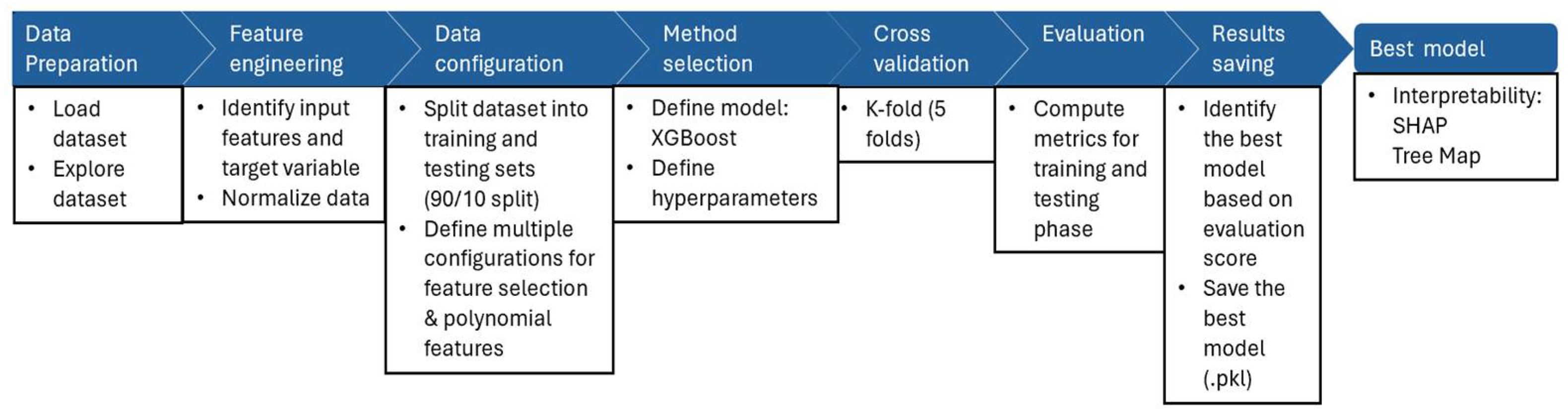
2.4. Modelling Techniques

The experimental data were loaded, checked and divided into training and test sets (Appendix A). The values for the input track overlapping and hatch spacing from the experimental data were omitted from the data used for modelling, as these values did not change during the experiment and could lead to skewing the model with invariant features. The relative density compared to the volumetric mass density of magnesium of 1.738 [g/cm3] was selected as the output value and expressed as a percentage for better readability. The modelling workflow is presented in Figure 3.

As mentioned, XGBoost was used as a fundamental method for the modelling framework. XGBoost is known as a powerful and scalable tree-boosting algorithm that has become a popular tool for regression tasks in ML for engineering applications. It uses a gradient boosting framework to iteratively refine prediction accuracy, outperforming traditional regression methods [23]. The specific parameters for the XGBoost used are defined in

Table 3. Parameters used for modelling with XGBoost.

Parameter	Values	Description
N estimators	[100, 200, 500]	Number of boosting rounds (trees) to fit
Max depth	[3, 5, 7]	Tree maximum depth, where a higher depth increases the model complexity
Learning rate	[0.01, 0.05, 0.1]	Step size shrinkage used to prevent overfitting, where smaller values slow down the model’s learning
Subsample	[0.6, 0.8, 1.0]	Proportion of the training data that was randomly selected for each boosting round; this was used to reduce overfitting
Alpha	[0, 0.1, 0.5]	L1 regularisation term used to control the parsimony of the model, where larger alpha values lead to a stronger regularization
Lambda	[1, 1.5, 2]	L2 regularisation term used to control the resulting model complexity, where larger lambda values penalise large coefficients

.

These parameter settings were chosen with the aim of achieving a balance between model performance, generalisation and computational efficiency. The range of values for each parameter allowed a comprehensive search in the hyperparameter space to determine the optimal combination.

2.5. Feature Importances Determination Logic

For the resulting models, the feature importances were determined through a systematic two-phase approach using feature engineering (FE) and polynomial features (PFs). Initially, scikit-learn’s polynomial features (up to the 2nd degree) [32] were employed to generate interaction terms such as “laser power × scanning speed” from the selected process parameters. Those terms were then integrated into the model pipeline when PFs were enabled, followed by a recursive feature elimination [33] with Elastic Net [34] to select key importances only. After training the XGBoost model with this extended set, the feature importances (FIs) were extracted using the “gain” metric that quantified the average contribution of each feature. These values were then normalised so that they summed to 1. They were assigned to the corresponding feature and expressed as percentages for direct interpretability. In addition, SHAP (SHapley Additive exPlanations) values were calculated to interpret the model’s predictions and depict feature importances [35].

3. Results

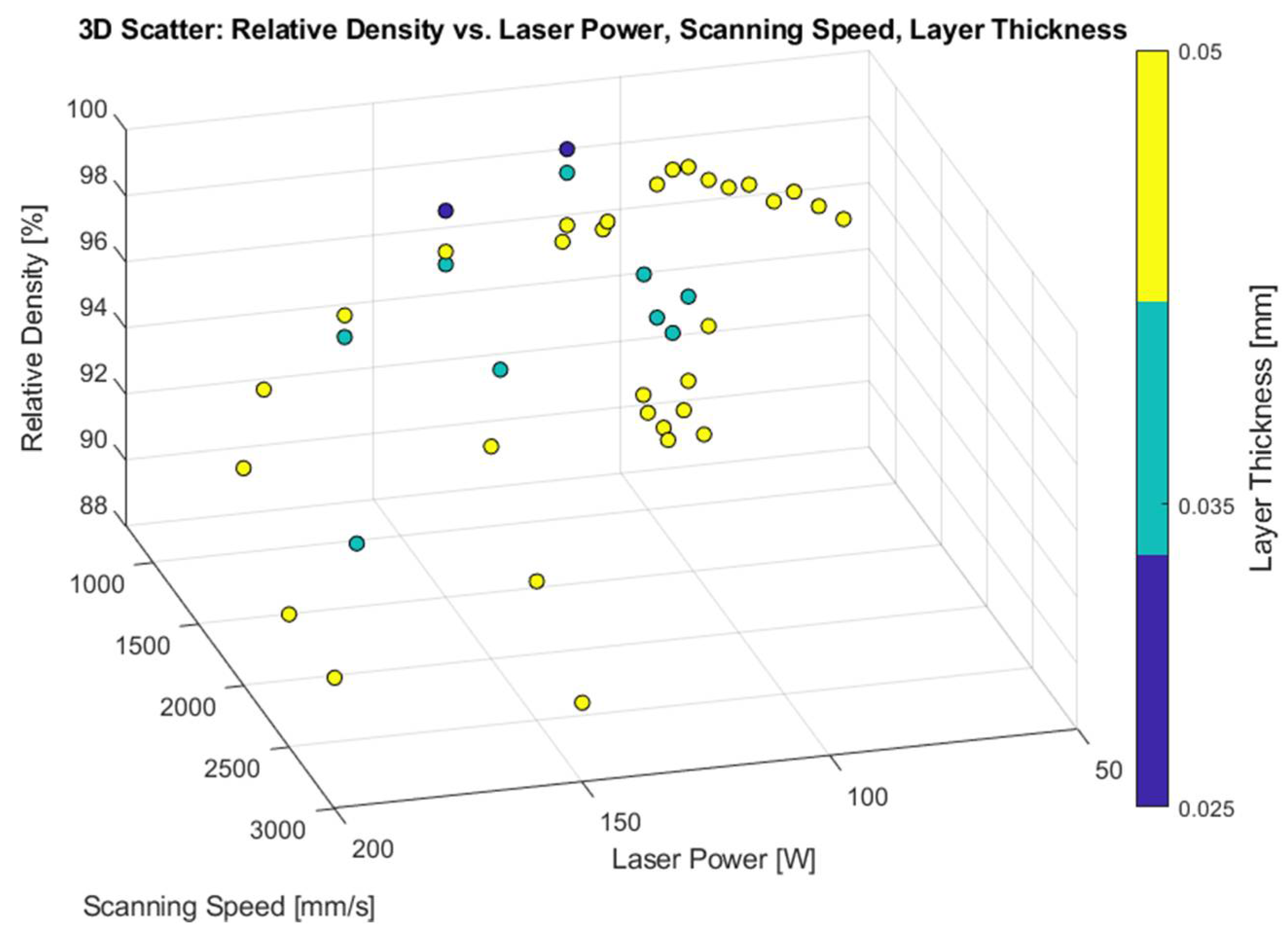
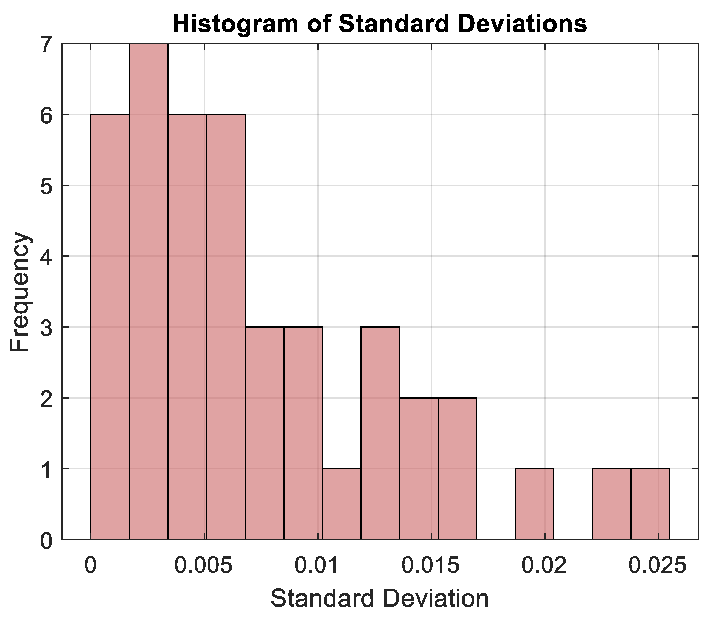
3.1. Measuring Results

The results obtained are presented in Table A1; for a better understanding of the relationships between the process parameters and the relative density, see Figure 4.

The 3D scatter plot (Figure 3) shows the correlations between the relative density and selected process parameters—laser power, scanning speed and layer thickness—from a data set of 42 points.

The x-axis indicates the laser power, which ranges from 100 to 200 W; the y-axis indicates the scanning speed, which ranges from 500 to 3000 mm/s; and the z-axis indicates the relative density, which ranges from 88% to 100%, with higher values indicating better material consolidation. The layer thickness is colour coded: 0.025 mm (purple), 0.035 mm (turquoise) and 0.05 mm (yellow). This shows that the highest relative densities (up to 100%) are achieved with the thinnest layer (0.025 mm), especially at moderate laser power (100–150 W) and scanning speeds (1000–2000 mm/s).

The graph shows an accumulation of points with high densities (95–100%) for 0.035 mm and 0.05 mm thin films in comparable parameter ranges, while lower densities (88–92%) occur at higher scanning speeds (e.g., 2500–3000 mm/s).

Standard Deviations

The distribution of standard deviations within a data set is represented by the histogram (Figure 5). The y-axis shows the frequency of occurrence, which ranges from 0 to 7, while the x-axis shows the standard deviation values, which range from 0 to 0.025. The data are categorised into bins, and the standard deviations between 0 and 0.005 have the highest frequencies (around 6–7). With values of around 3 for the 0.01 bin, 2 for the 0.015 bin and 1 for the 0.02 and 0.025 bins, the frequencies gradually decrease with larger standard deviations. This means that there are fewer examples of higher variability and that most of the data points have a low standard deviation, indicating relatively low variability.

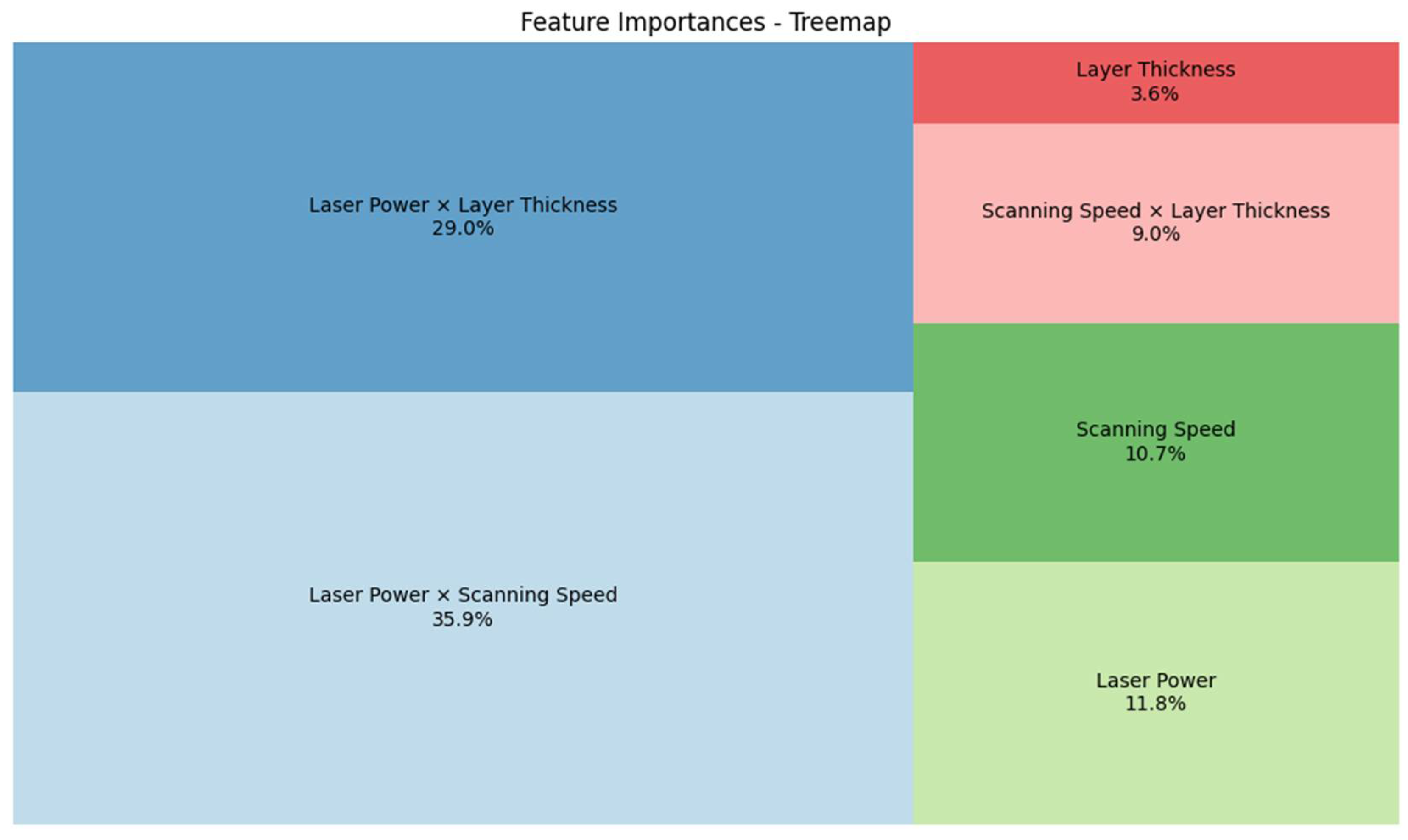
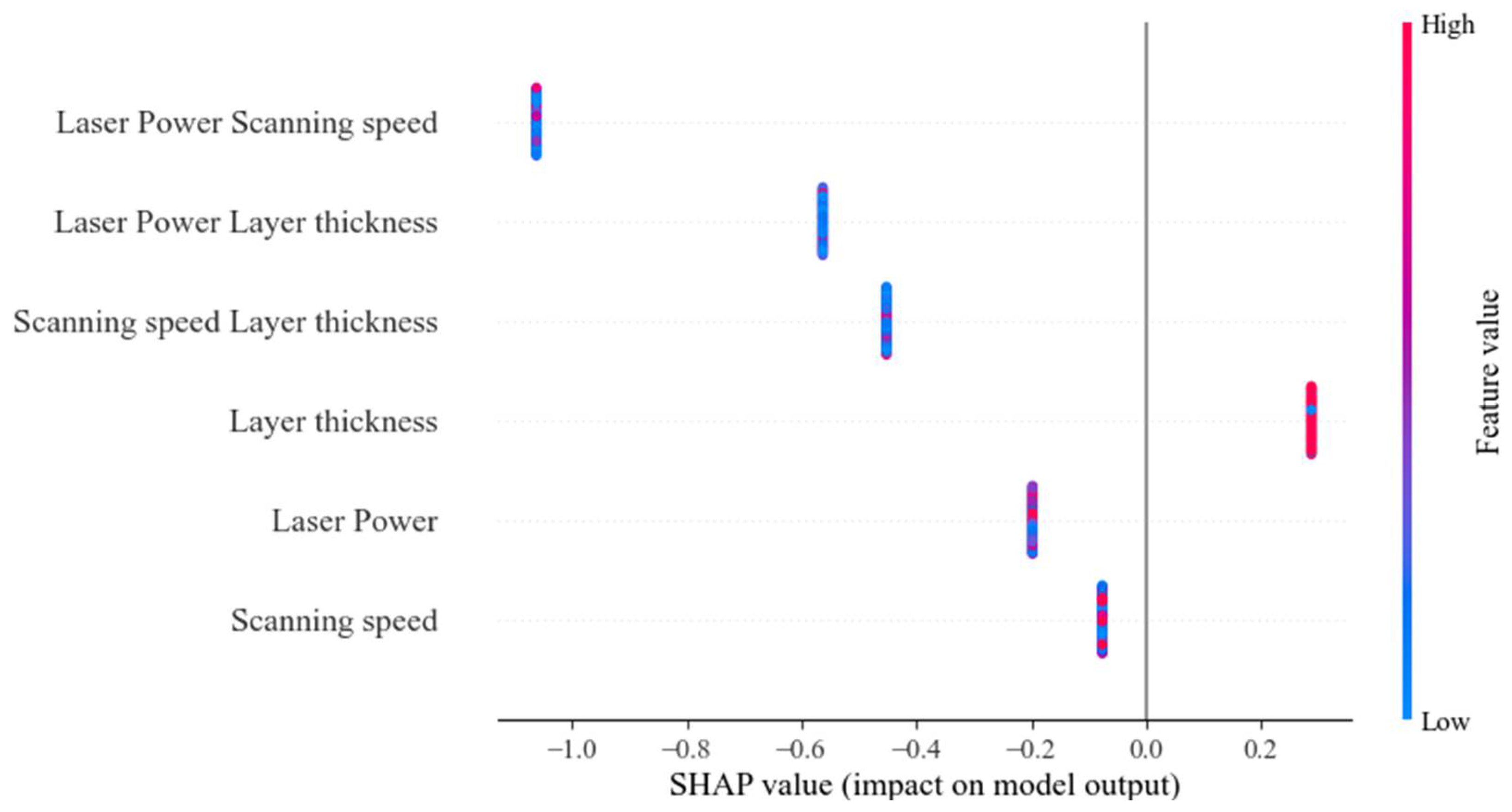
3.2. Feature Importances

FIs highlight the most important factors for the model’s created predictions (adding up to 100%):

• Laser power × scanning speed: 35.9%—proved to be the most influential feature, indicating that this interaction strongly influences the product density;
• Laser power × layer thickness: 29.0%—the second most important relationship, pointing to another critical interaction;
• Laser power: 11.8%—moderate standalone impact;
• Scanning speed: 10.7%—moderate individual contribution;
• Scanning speed × layer thickness: 9.0%—secondary interaction effect;
• Layer thickness: 3.6%—least influential on its own, but relevant in interactions.

In addition, the results for the FIs are visualised in Figure 6 with the help of tree mapping. This visualisation illustrates the relative importances of the individual features used in the model. Each block in the tree map corresponds to a specific feature, and its size is proportional to the influence of the feature on the model’s predictions. In other words, the larger the block, the more important the feature is for the outcome of the model.

The dominance of the generated interaction terms (together: 73.8%) over the individual features (26.2%) emphasises the usefulness of the selected methods, which leads to a successful capture of the complex relationships in the experimental data.

Laser power × scanning speed (35.9%) was found to be the most influential feature. This interaction represents the product of laser power (W) and scanning speed (mm/s) and has an indirect influence on energy density. The results show that higher values tend to increase the relative density of the product, probably due to improved fusion. However, the trend is not linear. For example, at a laser power of 120 W and a scanning speed of 1200 mm/s (product = 144,000), the relative density is 99.263% (improvement compared to [36]), while at 200 W and 2500 mm/s (product = 500,000) it drops to 92.016% (track overlapping, hatch spacing and layer thickness are the same for both). The data show that the relative density increases from 90% to 98% as the product of the chosen parameters increases from 50,000 to 200,000, but decreases beyond 400,000, probably due to over melting.

Laser power × layer thickness (29.0%): A higher power with thinner layers of material ensures more complete melting, which improves density, while thicker layers with insufficient power lead to voids. For example, at a power of 120 W (all other influencing factors at the same value) and a layer thickness of 0.035 mm, the resulting relative density is 99.263%, while at a layer thickness of 0.025 mm, the product has a relative density of 99.975%. The results show a steady increase in relative density with increasing power, with a steeper gradient at thinner layers (e.g., 0.025 mm). However, not enough layer thickness settings are used for definitive conclusions.

Laser power (11.8%): As an independent characteristic, the laser power contributes directly to the energy density. The analysis shows that increasing the laser power generally increases the relative density of the products, as more energy is available for melting the material. For example, at 65 W, the relative density is 95.952%, while at 55 W, it is 94.959% (the other inputs are left at the same values). However, even if a higher power provides more energy for melting, its effect alone is less significant if the speed or layer thickness is not taken into account.

Scanning speed (10.7%) has been shown to have the opposite effect on energy density, as it shortens the duration of the interaction of the laser beam with the material particles. Higher scanning speeds generally lead to a lower relative density of the product, as less energy is supplied. For example, at 1100 mm/s (laser power 100 W, layer thickness 0.035 mm, hatch spacing 0.035 mm, ED 51.948 J/mm³), the relative density was 94.183%, but at 3000 mm/s (laser power 150 W, layer thickness 0.05 mm, hatch spacing 0.035 mm, ED 42.857 J/mm³), it dropped to 90.399%, as there was not enough energy available for complete fusion of the material particles. This can be mitigated by increasing the laser power, as can be seen at 3000 mm/s with 200 W (ED 47.619 J/mm³), where the relative density improved to 91.556%. However, the results show that high energy densities can deliver excellent results at moderate speeds: At 1200 mm/s (laser power 120 W, layer thickness 0.025 mm, hatch spacing 0.035 mm, ED 114.286 J/mm³), the relative density reached 99.975%, showing that the material could tolerate high EDs with optimised parameters. For the product result at 950 mm/s (100 W laser power, 0.05 mm layer thickness, 0.035 mm hatch spacing, ED 60.150 J/mm³), the relative density dropped to 91.283%, which was probably due to process instabilities or over melting, and underlined the need for optimised parameters and further investigations.

Scanning speed × layer thickness (9.0%): The results showed that higher values reduced the relative density of the product. For example, at a scanning speed of 3000 mm/s and a layer thickness of 0.05 mm (product = 150), the relative density was 90.399%, while at 1500 mm/s and 0.035 mm (product = 35), it was 98.08 (all other factors remaining constant). Faster scanning with thicker layers reduced the energy density used, leading to problems with penetration and reduced particle melt quality.

Layer thickness (3.6%) was found to be the least influential independent parameter. Thicker layers reduce the relative density slightly, as they require more energy to melt the entire material. For example, the relative density at a layer thickness of 0.025 mm (laser power 120 W, scanning speed 1200 mm/s) was 99.975%, while at 0.035 mm (same power, hatch spacing, track overlapping and speed), it was 99.263. Furthermore, the results show that the relative density decreased from 98% to 96% when the layer thickness was increased from 0.025 mm to 0.05 mm.

Figure 7 shows the summarised SHAP representation, which quantifies the contributions of each input feature to the predicted part density in the model. The horizontal axis represents SHAP values that indicate the magnitude and direction of the effect of each feature on the output: positive values reflect a contribution to a higher predicted density, while negative values indicate a decrease. The features are arranged vertically in order of general importance. Each point corresponds to a single instance of data, with the colour representing the actual value of the feature—blue for low and red for high.

The diagram shows that the interaction terms laser power × scanning speed and laser power × layer thickness had the greatest influence on the result. Both show predominantly positive SHAP values, especially at higher feature values (shown in red), indicating that an increase in these combined parameters generally leads to a higher predicted density. This likely reflects the increased energy input and improved fusion conditions achieved under such settings. The interaction term scanning speed × layer thickness also shows a relatively strong negative contribution at high values, suggesting that a high scanning speed combined with thicker layers may reduce the energy density, resulting in a lower part density.

Individual parameters such as laser power and scanning speed demonstrate moderate effects, with SHAP values closer to zero and a more balanced distribution of positive and negative contributions. Remarkably, layer thickness as a single parameter shows the smallest impact, with SHAP values close to zero. This indicates that layer thickness alone does not have a large influence on the predicted density, and its effect becomes significant mainly through interactions with other variables. Overall, the SHAP analysis emphasises the dominant role of interactions between parameters in determining part quality and highlights the non-linear relationships captured by the model.

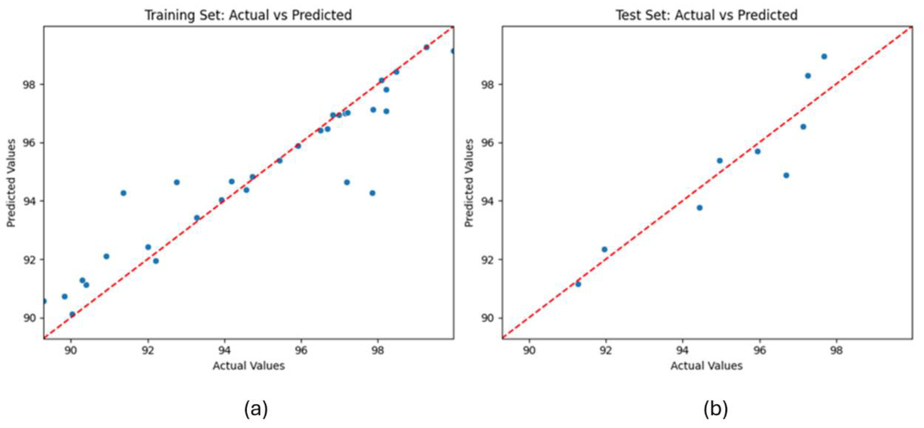
3.3. Model Performance Results

The XGBoost model demonstrated strong predictive performance (

Table 4. Metrics for the best model achieved.

Metric	Training	Testing
R2 Score	0.872	0.835
MAE	0.683	0.728
RMSE	1.118	0.892
MAPE	0.73%	0.76%
Pearson’s correlation coefficient	0.941	0.929

). It explained 83.5% of the variance in the test data set, indicating strong generalisation to different data while showing a small variation in the testing phase, indicating minimal overfitting. Pearsons’s value showed a robust linear correlation between predicted and actual densities, emphasising reliability. RMSE values revealed a moderate level of error. These metrics indicated that the model accurately forecasted the target variable (relative density), maintaining a balance between model accuracy and generalisation. The performance of the model can be compared with that of a similar method applied in [37], as it has better RMSE and MAE values, but has a worse R² score, showing space for improvement.

The resulting XGBoost model achieved usable results (test R²: 0.835, MAE: 0.728) while showing a significant dependence on influence interactions, especially on laser power × scan speed (35.9%) and laser power × layer thickness (29.0%), which enabled it to model complex patterns in the experimental data set effectively. The expected versus actual values of relative density for the training and test sets are shown in Figure 8.

The scatter plots present the model’s effectiveness when forecasting the relative density (89.29–99.975%). The training set (a) depicts a strong match, with the points tightly clustered around the ideal line (y = x). The test set (b) had shown some variability at the extreme values (90–92% and 98–99%) showing places for potential additional research. The slight reduction in R², which is addressed using regularisation, additionally emphasises the need for additional data to improve precision.

4. Discussion

This research presents XGBoost for predicting relative density in the LPBF AM of Mg. A key finding is that parameter interaction terms accounted for 73.8% of the model’s predictive importance, indicating that non-linear dependencies between process variables dominate density outcomes. This aligns with previous research showing that interactions significantly influence energy input and melt pool behaviour in LPBF processes [38,39], but it also extends the current understanding by quantifying these effects specifically for pure Mg using SHAP-based feature interaction analysis.

In general, higher laser power led to improved density due to higher energy input, which is consistent with findings in the literature that higher power improves fusion but risks overheating if the balance is insufficient [39]. Scanning speed showed a negative correlation with density, where higher values reduced the interaction time between laser energy and material, while moderate speeds combined with adequate power gave the best results. Layer thickness had a negligible direct effect, but showed higher density at lower values, which is consistent with studies showing that thinner layers improve fusion and surface quality [40].

The XGBoost model showed robust results; minor performance weaknesses at the edges could be due to process inconsistencies such as excessive melting or insufficient fusion, which, according to Heiss et al., are known problems with LPBF [38]. Importantly, SHAP analysis not only confirmed the dominance of interaction features but also offered interpretable insights, making the model useful for practical process optimisation—a step beyond traditional black-box predictions underpinning previous research that has used ML to investigate the complicated, non-linear dynamics of AM processes [39].

Study Limitations

Nevertheless, some limitations must be acknowledged. The low variability of layer thicknesses limits the understanding of the effects of this parameter. In addition, external influences—such as powder structure, environmental conditions or material-specific properties—were not considered in the modelling phase, as emphasised in more extensive AM reviews [40]. Future research should include a wider range of process parameters and evaluate the ability of the model to predict other characteristics such as microhardness and wear resistance, which are similarly affected by LPBF conditions [39].

The measured density range (89.29–99.975%) indicates optimised LPBF conditions; however, lower densities may occur in practise due to defects such as porosity. The accuracy of the XGBoost model (R²: 0.835) may decrease at lower density ranges (<89%) due to insufficient training data in this range. In future experiments, parameter adjustments leading to lower densities (e.g., higher scanning speeds or lower laser power) should be made and added to the training data to improve the robustness of the model.

The lack of a structured design of experiments (DOE) approach weakens the statistical validity of the findings, especially concerning interaction effects and the optimisation of parameter combinations. The grid-based method, although organised, might not investigate the multidimensional parameter space in full or consider the non-linear interactions among variables. Moreover, because of limitations in machine time and material access, the variety of test conditions was restricted, which could hinder the applicability of the findings.

5. Conclusions

In this study, XGBoost was effectively used to predict the relative density of pure magnesium components produced by Laser Powder Bed Fusion (LPBF). A significant finding was the identification of parameter interactions as the main factors accounting for 73.8% of the total feature importance, with laser power × scan speed identified as the most influential interaction affecting component density. In terms of individual effects, higher laser power typically increased density, while scanning speeds that were too high decreased it—results consistent with established LPBF behaviour but quantified here for the first time for pure magnesium.

The model showed that layer thickness had a small independent effect, although thinner layers tended to have higher densities. These findings confirm both established trends and the added value of explainable machine learning in uncovering subtle parameter interactions that influence part quality. The SHAP-based evaluation also provided clear visual representations that can contribute to informed process adjustments in future experiments or industrial applications.

Despite these encouraging results, the prediction accuracy showed some variance at the edges of the parameter space, probably due to the sparse data distribution and possible process instabilities, such as balling or insufficient fusion. Extending the data set through further experimental trials—especially for less studied parameter combinations—will improve the reliability and versatility of the model.

Future research should attempt to incorporate additional factors such as oxygen content in the build chamber, powder particle size distribution and post-processing procedures, which are known to influence LPBF results but were not addressed in this study. Furthermore, the inclusion of real-time monitoring systems (e.g., melt pool imaging and in situ thermal data) could improve the data richness and applicability of the models and ultimately enable a more reliable and scalable use of magnesium in additive manufacturing for structural or biomedical applications.

References

1. Chowdhury, S.; Yadaiah, N.; Prakash, C.; Ramakrishna, S.; Dixit, S.; Gupta, L.R.; Buddhi, D. Laser Powder Bed Fusion: A State-of-the-Art Review of the Technology, Materials, Properties & Defects, and Numerical Modelling. J. Mater. Res. Technol. 2022, 20, 2109–2172. [Google Scholar] [CrossRef]
2. Wang, C.; Shuai, Y.; Yang, Y.; Zeng, D.; Liang, X.; Peng, S.; Shuai, C. Amorphous Magnesium Alloy with High Corrosion Resistance Fabricated by Laser Powder Bed Fusion. J. Alloys Compd. 2022, 897, 163247. [Google Scholar] [CrossRef]
3. Wu, X.; Liu, J.; Yang, Y.; Bai, J.; Shuai, C.; Buhagiar, J.; Ning, X. Laser Powder Bed Fusion of Biodegradable Magnesium Alloys: Process, Microstructure and Properties. Int. J. Extrem. Manuf. 2025, 7, 022007. [Google Scholar] [CrossRef]
4. Kurzynowski, T.; Pawlak, A.; Smolina, I. The Potential of SLM Technology for Processing Magnesium Alloys in Aerospace Industry. Arch. Civ. Mech. Eng. 2020, 20, 23. [Google Scholar] [CrossRef]
5. Kulekci, M.K. Magnesium and Its Alloys Applications in Automotive Industry. Int. J. Adv. Manuf. Technol. 2008, 39, 851–865. [Google Scholar] [CrossRef]
6. Mordike, B.L.; Ebert, T. Magnesium: Properties—Applications—Potential. Mater. Sci. Eng. A 2001, 302, 37–45. [Google Scholar] [CrossRef]
7. Wu, C.L.; Xie, W.J.; Man, H.C. Laser Additive Manufacturing of Biodegradable Mg-Based Alloys for Biomedical Applications: A Review. J. Magnes. Alloys 2022, 10, 915–937. [Google Scholar] [CrossRef]
8. Haas, F.; Tiefnig, R.; Braun, M.; Taschauer, M.; Steinacker, S. Process Development and Risk Assessment for Processing Magnesium Alloys Using LPBF Technology. BHM Berg- Hüttenmänn. Monatshefte 2025, 170, 132–139. [Google Scholar] [CrossRef]
9. Qin, Y.; Wen, P.; Guo, H.; Xia, D.; Zheng, Y.; Jauer, L.; Poprawe, R.; Voshage, M.; Schleifenbaum, J.H. Additive Manufacturing of Biodegradable Metals: Current Research Status and Future Perspectives. Acta Biomater. 2019, 98, 3–22. [Google Scholar] [CrossRef]
10. Sharma, S.K.; Grewal, H.S.; Saxena, K.K.; Mohammed, K.A.; Prakash, C.; Davim, J.P.; Buddhi, D.; Raju, R.; Mohan, D.G.; Tomków, J. Advancements in the Additive Manufacturing of Magnesium and Aluminum Alloys through Laser-Based Approach. Materials 2022, 15, 8122. [Google Scholar] [CrossRef]
11. Zeng, Z.; Salehi, M.; Kopp, A.; Xu, S.; Esmaily, M.; Birbilis, N. Recent Progress and Perspectives in Additive Manufacturing of Magnesium Alloys. J. Magnes. Alloys 2022, 10, 1511–1541. [Google Scholar] [CrossRef]
12. Hwang, Y.J.; Kim, K.S.; AlMangour, B.; Grzesiak, D.; Lee, K.A. A New Approach for Manufacturing Stochastic Pure Magnesium Foam by Laser Powder Bed Fusion: Fabrication, Geometrical Characteristics, and Compressive Mechanical Properties. Adv. Eng. Mater. 2021, 23, 2100483. [Google Scholar] [CrossRef]
13. Simson, D.; Subbu, S.K. Effect of Process Parameters on Surface Integrity of LPBF Ti6Al4V. Procedia CIRP 2022, 108, 716–721. [Google Scholar] [CrossRef]
14. Shrivastava, A.; Anand Kumar, S.; Rao, S.; Nagesha, B.K. Exploring How LPBF Process Parameters Impact the Interface Characteristics of LPBF Inconel 718 Deposited on Inconel 718 Wrought Substrates. Opt. Laser Technol. 2024, 174, 110571. [Google Scholar] [CrossRef]
15. Bergmueller, S.; Gerhold, L.; Fuchs, L.; Kaserer, L.; Leichtfried, G. Systematic Approach to Process Parameter Optimization for Laser Powder Bed Fusion of Low-Alloy Steel Based on Melting Modes. Int. J. Adv. Manuf. Technol. 2023, 126, 4385–4398. [Google Scholar] [CrossRef]
16. Shrestha, S.; Chou, K. Formation of Keyhole and Lack of Fusion Pores during the Laser Powder Bed Fusion Process. Manuf. Lett. 2022, 32, 19–23. [Google Scholar] [CrossRef]
17. Qu, M.; Guo, Q.; Escano, L.I.; Clark, S.J.; Fezzaa, K.; Chen, L. Mitigating Keyhole Pore Formation by Nanoparticles during Laser Powder Bed Fusion Additive Manufacturing. Addit. Manuf. Lett. 2022, 3, 100068. [Google Scholar] [CrossRef]
18. Guo, L.; Wang, H.; Liu, H.; Huang, Y.; Wei, Q.; Leung, C.L.A.; Wu, Y.; Wang, H. Understanding Keyhole Induced-Porosities in Laser Powder Bed Fusion of Aluminum and Elimination Strategy. Int. J. Mach. Tools Manuf. 2023, 184, 103977. [Google Scholar] [CrossRef]
19. Liu, J.; Wen, P. Metal Vaporization and Its Influence during Laser Powder Bed Fusion Process. Mater. Des. 2022, 215, 110505. [Google Scholar] [CrossRef]
20. Equbal, M.A.; Equbal, A.; Khan, Z.A.; Badruddin, I.A. Machine Learning in Additive Manufacturing: A Comprehensive Insight. Int. J. Lightweight Mater. Manuf. 2025, 8, 264–284. [Google Scholar] [CrossRef]
21. Silbernagel, C.; Aremu, A.; Ashcroft, I. Using Machine Learning to Aid in the Parameter Optimisation Process for Metal-Based Additive Manufacturing. Rapid Prototyp. J. 2020, 26, 625–637. [Google Scholar] [CrossRef]
22. Liu, Q.; Wu, H.; Paul, M.J.; He, P.; Peng, Z.; Gludovatz, B.; Kruzic, J.J.; Wang, C.H.; Li, X. Machine-Learning Assisted Laser Powder Bed Fusion Process Optimization for AlSi10Mg: New Microstructure Description Indices and Fracture Mechanisms. Acta Mater. 2020, 201, 316–328. [Google Scholar] [CrossRef]
23. Chen, T.; Guestrin, C. XGBoost: A Scalable Tree Boosting System. In Proceedings of the ACM SIGKDD International Conference on Knowledge Discovery and Data Mining, Toronto, ON, Canada, 13 August 2016; Association for Computing Machinery. Volume 13–17, pp. 785–794. [Google Scholar]
24. Zou, M.; Jiang, W.G.; Qin, Q.H.; Liu, Y.C.; Li, M.L. Optimized XGBoost Model with Small Dataset for Predicting Relative Density of Ti-6Al-4V Parts Manufactured by Selective Laser Melting. Materials 2022, 15, 5298. [Google Scholar] [CrossRef]
25. Kruth, J.-P.; Leu, M.C.; Nakagawa, T. Progress in Additive Manufacturing and Rapid Prototyping. CIRP Ann. 1998, 47, 525–540. [Google Scholar] [CrossRef]
26. Yadroitsev, I.; Gusarov, A.; Yadroitsava, I.; Smurov, I. Single Track Formation in Selective Laser Melting of Metal Powders. J. Mater. Process. Technol. 2010, 210, 1624–1631. [Google Scholar] [CrossRef]
27. Gong, H.; Rafi, K.; Gu, H.; Starr, T.; Stucker, B. Analysis of Defect Generation in Ti-6Al-4V Parts Made Using Powder Bed Fusion Additive Manufacturing Processes. Addit. Manuf. 2014, 1–4, 87–98. [Google Scholar] [CrossRef]
28. Thijs, L.; Verhaeghe, F.; Craeghs, T.; Van Humbeeck, J.; Kruth, J.-P. A Study of the Microstructural Evolution during Selective Laser Melting of Ti-6Al-4V. Acta Mater. 2010, 58, 3303–3312. [Google Scholar] [CrossRef]
29. Gibson, I.; Rosen, D.; Stucker, B. Additive Manufacturing Technologies; Springer: New York, NY, USA, 2015; ISBN 978-1-4939-2112-6. [Google Scholar]
30. DebRoy, T.; Wei, H.L.; Zuback, J.S.; Mukherjee, T.; Elmer, J.W.; Milewski, J.O.; Beese, A.M.; Wilson-Heid, A.; De, A.; Zhang, W. Additive Manufacturing of Metallic Components—Process, Structure and Properties. Prog. Mater. Sci. 2018, 92, 112–224. [Google Scholar] [CrossRef]
31. Trevisan, F.; Calignano, F.; Lorusso, M.; Pakkanen, J.; Aversa, A.; Ambrosio, E.; Lombardi, M.; Fino, P.; Manfredi, D. On the Selective Laser Melting (SLM) of the AlSi10Mg Alloy: Process, Microstructure, and Mechanical Properties. Materials 2017, 10, 76. [Google Scholar] [CrossRef]
32. Bisong, E. Introduction to Scikit-Learn. In Building Machine Learning and Deep Learning Models on Google Cloud Platform; Apress: Berkeley, CA, USA, 2019; pp. 215–229. [Google Scholar]
33. Priyatno, A.M.; Widiyaningtyas, T. A Systematic Literature Review: Recursive Feature Elimination Algorithms. JITK (J. Ilmu Pengetah. Dan Teknol. Komput.) 2024, 9, 196–207. [Google Scholar] [CrossRef]
34. Zou, H.; Hastie, T. Regularization and Variable Selection Via the Elastic Net. J. R. Stat. Soc. Ser. B Stat. Methodol. 2005, 67, 301–320. [Google Scholar] [CrossRef]
35. Marcilio, W.E.; Eler, D.M. From Explanations to Feature Selection: Assessing SHAP Values as Feature Selection Mechanism. In Proceedings of the 2020 33rd SIBGRAPI Conference on Graphics, Patterns and Images (SIBGRAPI), Porto de Galinhas, Brazil, 7–10 November 2020; IEEE: New York, NY, USA, 2020; pp. 340–347. [Google Scholar]
36. Hu, D.; Wang, Y.; Zhang, D.; Hao, L.; Jiang, J.; Li, Z.; Chen, Y. Experimental Investigation on Selective Laser Melting of Bulk Net-Shape Pure Magnesium. Mater. Manuf. Process. 2015, 30, 1298–1304. [Google Scholar] [CrossRef]
37. Zhang, T.; Zhou, X.; Zhang, P.; Duan, Y.; Cheng, X.; Wang, X.; Ding, G. Hardness Prediction of Laser Powder Bed Fusion Product Based on Melt Pool Radiation Intensity. Materials 2022, 15, 4674. [Google Scholar] [CrossRef]
38. Heiss, A.; Thatikonda, V.S.; Klotz, U.E. Multi-Objective Optimization of LPBF Manufacturing with Zn-4Al-1Cu Alloy for Technical Applications. J. Manuf. Process. 2025, 134, 193–206. [Google Scholar] [CrossRef]
39. Barrionuevo, G.O.; Walczak, M.; Ramos-Grez, J.; Sánchez-Sánchez, X. Microhardness and Wear Resistance in Materials Manufactured by Laser Powder Bed Fusion: Machine Learning Approach for Property Prediction. CIRP J. Manuf. Sci. Technol. 2023, 43, 106–114. [Google Scholar] [CrossRef]
40. Chen, J.; Chen, B. Progress in Additive Manufacturing of Magnesium Alloys: A Review. Materials 2024, 17, 3851. [Google Scholar] [CrossRef]
Figure 1. Schematic of the manufacturing process.
Applsci 15 08592 g001
Figure 2. Arrow Metal Printing LMP200 (a), cubic samples (b), Axis analytical scale (c).
Applsci 15 08592 g002
Figure 3. Modelling workflow.
Applsci 15 08592 g003
Figure 4. Scatter plot of process parameters vs. the relative density.
Applsci 15 08592 g004
Figure 5. Histogram of standard deviations.
Applsci 15 08592 g005
Figure 6. Feature importances presented as a tree map.
Applsci 15 08592 g006
Figure 7. SHAP plot illustrating the features’ impacts.
Applsci 15 08592 g007
Figure 8. Predicted vs. actual relative density and scatter plots for (a) the training set and (b) the predictions of the test set.
Applsci 15 08592 g008