Research on the Cross-Efficiency Model of the Innovation Dynamic Network in China’s High-Tech Manufacturing Industry

Abstract

To evaluate the efficiency of innovation development in China’s high-tech manufacturing industry, this paper constructs a two-stage dynamic network cross-efficiency model. This model divides innovation activities into two stages: technology research and development and achievement transformation and introduces a 2-year lag period in the technology research and development stage and a 1-year lag period in the achievement transformation stage. It proposes the overall efficiency and efficiency models for each stage. The model was applied to 30 provinces in China, and the results showed that most provinces have achieved relatively ideal results in the overall efficiency and achievement transformation stage of high-tech manufacturing, while the efficiency in the technology research and development stage is generally lower than that in the achievement transformation stage. It is recommended that enterprises increase their R&D investments, break through technological barriers, and optimize the innovation chain.

1. Introduction

High-tech industry is the use of high technology for development and production, and it has become a key area in international economic and technological competition by virtue of its large R&D investment, high added value, good international market prospects, and far-reaching impacts on other industries, and its development plays an indispensable role in promoting the optimization and upgrading of the industrial structure [1]. Innovation has become a globally recognized important driving force, and the level of the high-tech industry is often regarded as one of the important indicators of the level of economic development. It is worth noting that not only limited to developed countries, emerging market countries have also increased investment in high-tech industry to enhance their own innovation capacity [2]. As a strategic leading industry in China, high-tech industry directly affects China’s national scientific and technological competitiveness and industrial core competitiveness [3], and innovation activities are the key driving force for competitive advantage, so the assessment of the innovation efficiency of China’s high-tech industry has attracted extensive attention.

High-tech industries can be further subdivided into high-tech manufacturing and high-tech service industries [4]. According to the Statistical Classification Directory of High-Tech Industries (Manufacturing) issued by the National Bureau of Statistics of China in 2013, China’s high-tech industries (manufacturing) are classified into six industries, namely, the pharmaceutical manufacturing industry; the aviation, spacecraft, and equipment manufacturing industry; the electronics and communication equipment manufacturing industry; the computer and office equipment manufacturing industry; medical instrumentation and instrumentation manufacturing; and information chemicals manufacturing. Therefore, this study attempts to investigate the efficiency of innovation activities in China’s provincial high-tech manufacturing industries and to provide a corresponding basis for decision making.

Currently, there are many assessment methods for the development of the high-tech industry. Yu et al. explored the key factors of the ecological development of the high-tech industry based on hierarchical analysis [5]. Meng, L. and Sun, L.Y. explored the influence relationship of the technological innovation efficiency of the high-tech industry through factor analysis and multiple-regression analysis [6]. Gui, J.Y. used the improved CRITIC objective assignment method to assign weights to the indicators and graded the development level of high-tech industries in 31 provinces (cities and districts) of China by the non-integer rank-order sum ratio method WRSR [7]. Chen, X.X. and Shi, D.H. used the comprehensive index method to measure the high-quality comprehensive development index of high-tech industries in 30 provinces (municipalities and autonomous regions) in China [8]. Wang, Z.X. et al. used the improved TOPSIS method to assess the provincial competitiveness of China’s high-tech industries [9]. Wang, R.D. and Zhang, J.J. measured the global industrial chain level of China’s provincial high-tech industry by the entropy value method–TOPSIS method [10].

The most commonly used method to assess the innovation efficiency of high-tech industries is data envelopment analysis (DEA) [11,12]. First of all, the traditional DEA model has the characteristic of a “black box”, and some scholars believe that China’s high-tech innovation activities should be divided into two processes: the R&D stage and the commercialization stage [13,14]. On this basis, some scholars consider the initial inputs in the R&D stage, the additional inputs in the commercialization stage, and the shared inputs between the two stages [15,16,17]. Second, the traditional DEA model is still a static model. In order to solve the problem, Lin et al. used DEA window analysis with an ideal window width to dynamically assess the technological innovation efficiency of China’s high-tech industry [18], and some scholars combined the traditional DEA model with the Malmquist index model to dynamically measure the innovation efficiency of China’s high-tech industry [19,20,21]. Meanwhile, the traditional DEA model has the problem of the self-assessment mode, and Wang, Q.J. et al. evaluated the efficiency of R&D activities in regional high-tech industries by combining the two-stage DEA model with the cross-DEA model [22].

Most of the models in the above-mentioned studies only focus on improving one or two major issues in the DEA basic model, failing to simultaneously address its multiple core problems. They also do not fully consider factors such as shared input, the impacts of different stages, and the time lag effect, which are of great significance in practical applications. From the above, it can be seen that current research and development should pay more attention to constructing dynamic network cross-efficiency models to make up for these deficiencies and improve the application effect of DEA models in complex environments.

Therefore, this paper adopts the panel data of China’s high-tech manufacturing industry, divides the innovation activities of the high-tech manufacturing industry into the stage of technology R&D and the stage of result transformation, and, at the same time, takes into account the initial input of the first stage, the additional input of the second stage, the shared input of the two stages, as well as the efficiency of the R&D lag, to construct a two-stage dynamic network cross-efficiency model and conduct an empirical study on the innovation efficiency of the high-tech manufacturing industry of different provinces in China. We construct a two-stage dynamic network cross-efficiency model to empirically investigate the innovation efficiency of high-tech manufacturing industries in different provinces of China and study the innovation efficiency in the technology R&D stage as well as the achievement transformation stage.

2. Research Methods

2.1. Cross-Efficiency Model

In order to solve the problems of the self-assessment mode of the traditional DEA evaluation model and the inability to fully order the decision units, Sexton et al. proposed a cross-efficiency evaluation method that combines self-assessment and mutual assessment [23], which first utilizes the traditional DEA model to obtain the decision unit’s own efficiency and the optimal weight and then combines them with a set of the optimal weights of all the decision units to evaluate the cross-efficiency of each decision unit. The cross-efficiency based on the CCR model is taken as an example here.

Suppose that there are n homogeneous decision-making units $DM{U}_d(d=1,\dots ,n)$, each with I inputs and M outputs, $x_{id}$ denotes the ith input of the $DM{U}_d$, and $y_{md}$ denotes the mth output of the $DM{U}_d$; $u_{id}$ is the weight of the ith input, and $v_{md}$ is the weight of the mth output. Assuming that the self-assessed efficiency value of the $DM{U}_d$ is ${\theta }_{dd}$, the following formulation is available:

$$\begin{array}{lll}\max & {\theta }_{dd}={\displaystyle \frac{{\displaystyle \sum _{m=1}^M{v}_{md}{y}_{md}}}{{\displaystyle \sum _{i=1}^I{u}_{id}{x}_{id}}}}& \\ s.t.& {\displaystyle \frac{{\displaystyle \sum _{m=1}^M{v}_{md}{y}_{mj}}}{{\displaystyle \sum _{i=1}^I{u}_{id}{x}_{ij}}}}\le 1,& d=1,\dots ,n\\ & u_{id}\ge 0,& i=1,\dots ,I\\ & v_{md}\ge 0,& m=1,\dots ,M\end{array}$$

(1)

Assuming that the optimal weights of the above model are $u_{id}^{*}$ and $v_{md}^{*}$, the cross-efficiency (${\theta }_{dj}$) of decision unit $DM{U}_j$ with respect to $DM{U}_d$ is

$$\begin{array}{ll}{\theta }_{dj}={\displaystyle \frac{{\displaystyle \sum _{m=1}^M{v}_{md}^{*}{y}_{mj}}}{{\displaystyle \sum _{i=1}^I{u}_{id}^{*}{x}_{ij}}}},& d,j=1,2,\dots ,n\end{array}$$

(2)

After each $DM{U}_d$ obtains a set of optimal weights through the traditional DEA model, all the weights are used to evaluate the efficiency of the decision unit ($DM{U}_j$) to obtain the cross-efficiency matrix ($\theta$).

$$\theta =\left[\begin{array}{cccc}{\theta }_{11}& {\theta }_{12}& \dots & {\theta }_{1n}\\ {\theta }_{21}& {\theta }_{22}& \dots & {\theta }_{2n}\\ \dots & \dots & \dots & \dots \\ {\theta }_{n1}& {\theta }_{n2}& \dots & {\theta }_{nn}\end{array}\right]$$

(3)

In the matrix, the dth row ($DM{U}_d$) evaluates the efficiency of all the decision units separately; the jth column represents the efficiency evaluation of the $DM{U}_j$ by all the decision units, so the cross-efficiency value (${\theta }_j$) of the $DM{U}_j$ can be taken as the arithmetic mean of all the efficiencies in the jth column.

$${\theta }_j={\displaystyle \frac{1}{n}}{\displaystyle \sum _{d=1}^n{\theta }_{dj}}$$

(4)

Since most weights obtained from the solution using the traditional DEA model may not be unique, this may lead to non-unique cross-efficiency values. To solve this problem, Dolye et al. introduced secondary objectives and proposed two strategic secondary objective models: adversarial type and benevolent type [24].

The linear programming form of the adversarial cross-efficiency model is as follows:

$$\begin{array}{lll}\min & {\displaystyle \sum _{m=1}^M({\xi }_{md}}{\displaystyle \sum _{j=1,j\ne d}^n{y}_{mj})}& \\ s.t.& {\displaystyle \sum _{i=1}^I({\mu }_{id}}{\displaystyle \sum _{j=1,j\ne d}^n{x}_{ij}})=1,& \\ & {\displaystyle \sum _{m=1}^M{\xi }_{md}}{y}_{md}-{\theta }_{dd}^{*}{\displaystyle \sum _{i=1}^I{\mu }_{id}}{x}_{id}=0,& \\ & {\displaystyle \sum _{m=1}^M{\xi }_{md}}{y}_{mj}-{\displaystyle \sum _{i=1}^I{\mu }_{id}}{x}_{ij}\le 0,& j=1,\dots ,n;j\ne d;\\ & {\xi }_{md}{y}_{md}-\delta \ge 0,& m=1,\dots ,M\\ & {\mu }_{id}\ge 0,& i=1,\dots ,I\\ & \delta \ge 0& \end{array}$$

(5)

The linear programming form of the benevolent cross-efficiency model is as follows:

$$\begin{array}{lll}\max & {\displaystyle \sum _{m=1}^M({\xi }_{md}}{\displaystyle \sum _{j=1,j\ne d}^n{y}_{mj})}& \\ s.t.& {\displaystyle \sum _{i=1}^I({\mu }_{id}}{\displaystyle \sum _{j=1,j\ne d}^n{x}_{ij}})=1,& \\ & {\displaystyle \sum _{m=1}^M{\xi }_{md}}{y}_{md}-{\theta }_{dd}^{*}{\displaystyle \sum _{i=1}^I{\mu }_{id}}{x}_{id}=0,& \\ & {\displaystyle \sum _{m=1}^M{\xi }_{md}}{y}_{mj}-{\displaystyle \sum _{i=1}^I{\mu }_{id}}{x}_{ij}\le 0,& j=1,\dots ,n;j\ne d;\\ & {\xi }_{md}{y}_{md}-\delta \ge 0,& m=1,\dots ,M\\ & {\mu }_{id}\ge 0,& i=1,\dots ,I\\ & \delta \ge 0& \end{array}$$

(6)

Under the premise of keeping the self-assessed efficiency value of the decision unit unchanged, the adversarial type is to minimize the average of the cross-efficiency values of the other decision units, and the benevolent type is to maximize the average of the cross-efficiency values of the other decision units, but it is not given how to choose these two secondary objectives. For this reason, Wang proposed the neutral-type secondary objective model [25]. The neutral cross-efficiency model no longer focuses on whether to maximize or minimize the average of the cross-efficiency values of the other decision units but rather on whether to make the decision unit’s own inputs and outputs of the zero-weight value of the minimum possible and whether the selected weights are convenient for calculating the efficiency value of the decision unit. The linear programming form of the neutral cross-efficiency model is as follows:

$$\begin{array}{lll}\max & \delta & \\ s.t.& {\displaystyle \sum _{i=1}^I{\mu }_{id}}{x}_{id}=1,& \\ & {\displaystyle \sum _{m=1}^M{\xi }_{md}}{y}_{md}={\theta }_{dd}^{*},& \\ & {\displaystyle \sum _{m=1}^M{\xi }_{md}}{y}_{mj}-{\displaystyle \sum _{i=1}^I{\mu }_{id}}{x}_{ij}\le 0,& j=1,\dots ,n;j\ne d;\\ & {\xi }_{md}{y}_{md}-\delta \ge 0,& m=1,\dots ,M\\ & {\mu }_{id}\ge 0,& i=1,\dots ,I\\ & \delta \ge 0& \end{array}$$

(7)

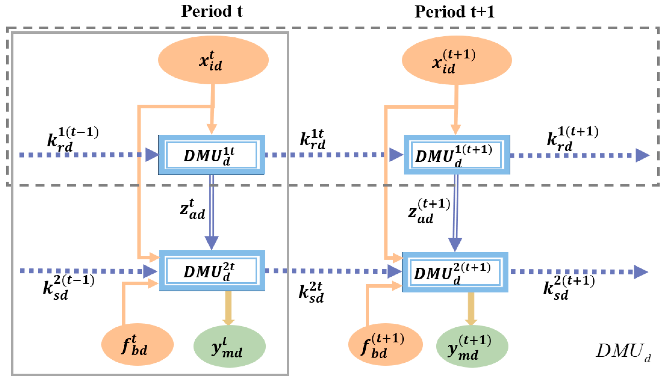
2.2. Two-Stage Dynamic Network Model

Suppose that the network structure is a classical two-stage network structure with T periods and n homogeneous decision units ($DM{U}_d(d=1,\dots ,n)$). $DM{U}_d^{Nt}$ is the Nth stage of $DM{U}_d$ in period t; $x_{id}^t$ is the ith shared input of $DM{U}_d$ in period t, where ${\alpha }_i^t$ is the proportion of sub-matches in stage one; $z_{ad}^t$ is the ath connecting variable between stage one and stage two of $DM{U}_d$ in period t; $k_{rd}^{1t}$ is the rth carry-over variable in stage one of $DM{U}_d$ in period t, and $k_{sd}^{2t}$ is the sth carry-over variable of $DM{U}_d$ in period t, stage two; $f_{bd}^t$ is the bth input of $DM{U}_d$ in period t, stage two; and $y_{md}^t$ is the mth output of $DM{U}_d$ in period t, stage two, where $d=1,\dots ,n$, $t=1,2,\dots ,T$, $N\in \{1,2\}$, $i=1,\dots ,I$, $a=1,\dots ,A$, $r=1,\dots ,R$, $s=1,\dots ,S$, $b=1,\dots ,B$, and $m=1,\dots ,M$. There is a mathematical structure of the model, as shown in Figure 1.

Based on the assumption of constant returns to scale, the linear programming form of the two-stage dynamic network DEA model is as follows:

$$\begin{array}{ll}\max & {\theta }_{dd}^{NT}={\displaystyle \sum _{t=1}^T\left({\displaystyle \sum _{a=1}^A{\delta }_{ad}}{z}_{ad}^t+{\displaystyle \sum _{r=1}^R{\psi }_{rd}^1}{k}_{rd}^{1t}+{\displaystyle \sum _{m=1}^M{\xi }_{md}}{y}_{md}^t+{\displaystyle \sum _{s=1}^S{\psi }_{sd}^2}{k}_{sd}^{2t}\right)}\\ s.t.& {\displaystyle \sum _{t=1}^T\left({\displaystyle \sum _{i=1}^I{\mu }_{id}}{x}_{id}^t+{\displaystyle \sum _{r=1}^R{\psi }_{rd}^1}{k}_{rd}^{1(t-1)}+{\displaystyle \sum _{a=1}^A{\delta }_{ad}}{z}_{ad}^t+{\displaystyle \sum _{b=1}^B{\zeta }_{bd}}{f}_{bd}^t+{\displaystyle \sum _{s=1}^S{\psi }_{sd}^2}{k}_{sd}^{2(t-1)}\right)}=1\\ & {\displaystyle \sum _{t=1}^T\left(\begin{array}{l}{\displaystyle \sum _{a=1}^A{\delta }_{ad}}{z}_{aj}^t+{\displaystyle \sum _{r=1}^R{\psi }_{rd}^1}{k}_{rj}^{1t}+\\ {\displaystyle \sum _{m=1}^M{\xi }_{md}}{y}_{mj}^t+{\displaystyle \sum _{s=1}^S{\psi }_{sd}^2}{k}_{sj}^{2t}\end{array}\right)}\\ & -{\displaystyle \sum _{t=1}^T\left(\begin{array}{l}{\displaystyle \sum _{i=1}^I{\mu }_{id}}{x}_{ij}^t+{\displaystyle \sum _{r=1}^R{\psi }_{rd}^1}{k}_{rj}^{1(t-1)}+\\ {\displaystyle \sum _{a=1}^A{\delta }_{ad}}{z}_{aj}^t+{\displaystyle \sum _{b=1}^B{\zeta }_{bd}}{f}_{bj}^t+{\displaystyle \sum _{s=1}^S{\psi }_{sd}^2}{k}_{sj}^{2(t-1)}\end{array}\right)}⩽0\hspace{1em}(j=1,\dots ,n)\\ & {\displaystyle \sum _{a=1}^A{\delta }_{ad}}{z}_{aj}^t+{\displaystyle \sum _{r=1}^R{\psi }_{rd}^1}{k}_{rj}^{1t}-\left({\displaystyle \sum _{i=1}^I{\tau }_{id}^t}{x}_{ij}^t+{\displaystyle \sum _{r=1}^R{\psi }_{rd}^1}{k}_{rj}^{1(t-1)}\right)⩽0\hspace{1em}\\ & (j=1,\dots ,n;t=1,\dots ,T)\\ & {\displaystyle \sum _{m=1}^M{\xi }_{md}}{y}_{mj}^t+{\displaystyle \sum _{s=1}^S{\psi }_{sd}^2}{k}_{sj}^{2t}-\left(\begin{array}{l}{\displaystyle \sum _{i=1}^I({\mu }_{id}-{\tau }_{id}^t)}{x}_{ij}^t+{\displaystyle \sum _{a=1}^A{\delta }_{ad}}{z}_{aj}^t\\ +{\displaystyle \sum _{b=1}^B{\zeta }_{bd}}{f}_{bj}^t+{\displaystyle \sum _{s=1}^S{\psi }_{sd}^2}{k}_{sj}^{2(t-1)}\end{array}\right)⩽0\hspace{1em}\\ & (j=1,\dots ,n;t=1,\dots ,T)\\ & L_i^t{\mu }_{id}⩽{\tau }_{id}^t⩽H_i^t{\mu }_{id}\hspace{1em}(i=1,\dots ,I;t=1,\dots ,T)\\ & {\mu }_{id}⩾0,{\delta }_{ad}⩾0,{\psi }_{rd}^1⩾0,{\psi }_{sd}^2⩾0,{\zeta }_{bd}⩾0,{\xi }_{md}⩾0\\ & (i=1,\dots ,I;a=1,\dots ,A;r=1,\dots ,R;s=1,\dots ,S;b=1,\dots ,B;m=1,\dots ,M)\end{array}$$

(8)

2.3. Two-Stage Dynamic Network Cross-Efficiency Model

Traditional DEA models are both black-box in nature (assessing the efficiency of a decision unit through external input and output data without considering the specific mechanisms of its internal processes) and static self-assessment models (not being able to assess the efficiency of a decision unit dynamically and uniquely). In addition, in practice, many production processes often contain multiple stages, and different stages may share the same input indicators, which makes the traditional DEA models have some limitations in dealing with such problems. In order to overcome these limitations, this paper proposes an innovative approach, combining neutral cross-efficiency and two-stage dynamic network modeling, which can effectively deal with two-stage production structures with shared inputs. The specific model is as follows:

$$\max W=\underset{\begin{array}{l}a\in \left\{1,\dots ,A\right\}\\ r\in \left\{1,\dots ,R\right\}\\ m\in \left\{1,\dots ,M\right\}\\ s\in \left\{1,\dots ,S\right\}\end{array}}{\min }{\displaystyle \frac{{\displaystyle \sum _{t=1}^T\left({\phi }_{ao}{z}_{ao}^t+{\varphi }_{ro}^1{k}_{ro}^{1t}+v_{mo}{y}_{mo}^t+{\varphi }_{so}^2{k}_{so}^{2t}\right)}}{{\displaystyle \sum _{t=1}^T\left({\displaystyle \sum _{i=1}^I{u}_{io}}{x}_{io}^t+{\displaystyle \sum _{r=1}^R{\varphi }_{ro}^1}{k}_{ro}^{1(t-1)}+{\displaystyle \sum _{a=1}^A{\phi }_{ao}}{z}_{ao}^t+{\displaystyle \sum _{b=1}^B{\eta }_{bo}}{f}_{bo}^t+{\displaystyle \sum _{s=1}^S{\varphi }_{so}^2}{k}_{so}^{2(t-1)}\right)}}}$$

(9)

$$\begin{array}{l}s.t.\\ {\displaystyle \frac{{\displaystyle \sum _{t=1}^T\left({\displaystyle \sum _{a=1}^A{\phi }_{ao}}{z}_{ad}^t+{\displaystyle \sum _{r=1}^R{\varphi }_{ro}^1}{k}_{rd}^{1t}+{\displaystyle \sum _{m=1}^M{v}_{mo}}{y}_{md}^t+{\displaystyle \sum _{s=1}^S{\varphi }_{so}^2}{k}_{sd}^{2t}\right)}}{{\displaystyle \sum _{t=1}^T\left({\displaystyle \sum _{i=1}^I{u}_{io}}{x}_{id}^t+{\displaystyle \sum _{r=1}^R{\varphi }_{ro}^1}{k}_{rd}^{1(t-1)}+{\displaystyle \sum _{a=1}^A{\phi }_{ao}}{z}_{ad}^t+{\displaystyle \sum _{b=1}^B{\eta }_{bo}}{f}_{bd}^t+{\displaystyle \sum _{s=1}^S{\varphi }_{so}^2}{k}_{sd}^{2(t-1)}\right)}}}={\theta }_{dd}^{NT*}\\ {\displaystyle \frac{{\displaystyle \sum _{t=1}^T\left({\displaystyle \sum _{a=1}^A{\phi }_{ao}}{z}_{aj}^t+{\displaystyle \sum _{r=1}^R{\varphi }_{ro}^1}{k}_{rj}^{1t}+{\displaystyle \sum _{m=1}^M{v}_{mo}}{y}_{mj}^t+{\displaystyle \sum _{s=1}^S{\varphi }_{so}^2}{k}_{sj}^{2t}\right)}}{{\displaystyle \sum _{t=1}^T\left({\displaystyle \sum _{i=1}^I{u}_{io}}{x}_{ij}^t+{\displaystyle \sum _{r=1}^R{\varphi }_{ro}^1}{k}_{rj}^{1(t-1)}+{\displaystyle \sum _{a=1}^A{\phi }_{ao}}{z}_{aj}^t+{\displaystyle \sum _{b=1}^B{\eta }_{bo}}{f}_{bj}^t+{\displaystyle \sum _{s=1}^S{\varphi }_{so}^2}{k}_{sj}^{2(t-1)}\right)}}}⩽1\hspace{1em}\\ (j=1,\dots ,n;j\ne 0)\\ {\displaystyle \frac{{\displaystyle \sum _{a=1}^A{\phi }_{ao}}{z}_{aj}^t+{\displaystyle \sum _{r=1}^R{\varphi }_{ro}^1}{k}_{rj}^{1t}}{{\displaystyle \sum _{i=1}^I{u}_{io}{\alpha }_i^t}{x}_{ij}^t+{\displaystyle \sum _{r=1}^R{\varphi }_{ro}^1}{k}_{rj}^{1(t-1)}}}⩽1\hspace{1em}(j=1,\dots ,n;t=1,\dots ,T)\\ \frac{{\displaystyle \sum _{m=1}^M{v}_{mo}}{y}_{mj}^t+{\displaystyle \sum _{s=1}^S{\varphi }_{so}^2}{k}_{sj}^{2t}}{{\displaystyle \sum _{i=1}^I{u}_{io}}\left(1-{\alpha }_i^t\right)x_{ij}^t+{\displaystyle \sum _{a=1}^A{\phi }_{ao}}{z}_{aj}^t+{\displaystyle \sum _{b=1}^B{\eta }_{bo}}{f}_{bj}^t+{\displaystyle \sum _{s=1}^S{\varphi }_{so}^2}{k}_{sj}^{2(t-1)}}⩽1\hspace{1em}\\ (j=1,\dots ,n;t=1,\dots ,T)\\ L_i^t{u}_{id}⩽{\alpha }_i^t{u}_{id}⩽H_i^t{u}_{id}\hspace{1em}(i=1,\dots ,I;t=1,\dots ,T)\\ u_{id}⩾0,{\phi }_{ad}⩾0,{\varphi }_{rd}^1⩾0,{\varphi }_{sd}^2⩾0,{\eta }_{bd}⩾0,v_{md}⩾0\\ u_{io}⩾0,{\phi }_{ao}⩾0,{\varphi }_{ro}^1⩾0,{\varphi }_{so}^2⩾0,{\eta }_{bo}⩾0,v_{mo}⩾0(o=1,\dots ,n and o\ne d)\\ (i=1,\dots ,I;a=1,\dots ,A;r=1,\dots ,R;s=1,\dots ,S;b=1,\dots ,B;m=1,\dots ,M)\end{array}$$

This model is equivalently transformed into the following linear programming form via the Charnes–Cooper transform [26].

$$\begin{gathered} \begin{array}{l}\max W\\ s.t.\\ {\displaystyle \sum _{t=1}^T\left(\begin{array}{l}{\displaystyle \sum _{a=1}^A{\delta }_{ao}}{z}_{ad}^t+{\displaystyle \sum _{r=1}^R{\psi }_{ro}^1}{k}_{rd}^{1t}+\\ {\displaystyle \sum _{m=1}^M{\xi }_{mo}}{y}_{md}^t+{\displaystyle \sum _{s=1}^S{\psi }_{so}^2}{k}_{sd}^{2t}\end{array}\right)}-{\theta }_{dd}^{NT*}\cdot {\displaystyle \sum _{t=1}^T\left(\begin{array}{l}{\displaystyle \sum _{i=1}^I{\mu }_{io}}{x}_{id}^t+{\displaystyle \sum _{r=1}^R{\psi }_{ro}^1}{k}_{rd}^{1(t-1)}+{\displaystyle \sum _{a=1}^A{\delta }_{ao}}{z}_{ad}^t\\ +{\displaystyle \sum _{b=1}^B{\zeta }_{bo}}{f}_{bd}^t+{\displaystyle \sum _{s=1}^S{\psi }_{so}^2}{k}_{sd}^{2(t-1)}\end{array}\right)}=0\\ {\displaystyle \sum _{t=1}^T\left({\displaystyle \sum _{i=1}^I{\mu }_{io}}{x}_{io}^t+{\displaystyle \sum _{r=1}^R{\psi }_{ro}^1}{k}_{ro}^{1(t-1)}+{\displaystyle \sum _{a=1}^A{\delta }_{ao}}{z}_{ao}^t+{\displaystyle \sum _{b=1}^B{\zeta }_{bo}}{f}_{bo}^t+{\displaystyle \sum _{s=1}^S{\psi }_{so}^2}{k}_{so}^{2(t-1)}\right)}=1\\ {\displaystyle \sum _{t=1}^T\left(\begin{array}{l}{\displaystyle \sum _{a=1}^A{\delta }_{ao}}{z}_{aj}^t+{\displaystyle \sum _{r=1}^R{\psi }_{ro}^1}{k}_{rj}^{1t}+\\ {\displaystyle \sum _{m=1}^M{\xi }_{mo}}{y}_{mj}^t+{\displaystyle \sum _{s=1}^S{\psi }_{so}^2}{k}_{sj}^{2t}\end{array}\right)}-{\displaystyle \sum _{t=1}^T\left(\begin{array}{l}{\displaystyle \sum _{i=1}^I{\mu }_{io}}{x}_{ij}^t+{\displaystyle \sum _{r=1}^R{\psi }_{ro}^1}{k}_{rj}^{1(t-1)}+{\displaystyle \sum _{a=1}^A{\delta }_{ao}}{z}_{aj}^t\\ +{\displaystyle \sum _{b=1}^B{\zeta }_{bo}}{f}_{bj}^t+{\displaystyle \sum _{s=1}^S{\psi }_{so}^2}{k}_{sj}^{2(t-1)}\end{array}\right)}⩽0\hspace{1em}\\ (j=1,\dots ,n)\\ {\displaystyle \sum _{a=1}^A{\delta }_{ao}}{z}_{aj}^t+{\displaystyle \sum _{r=1}^R{\psi }_{ro}^1}{k}_{rj}^{1t}-\left({\displaystyle \sum _{i=1}^I{\tau }_{io}^t}{x}_{ij}^t+{\displaystyle \sum _{r=1}^R{\psi }_{ro}^1}{k}_{rj}^{1(t-1)}\right)⩽0\hspace{1em}(j=1,\dots ,n;t=1,\dots ,T)\\ {\displaystyle \sum _{m=1}^M{\xi }_{mo}}{y}_{mj}^t+{\displaystyle \sum _{s=1}^S{\psi }_{so}^2}{k}_{sj}^{2t}-\left(\begin{array}{l}{\displaystyle \sum _{i=1}^I({\mu }_{io}-{\tau }_{io}^t)}{x}_{ij}^t+{\displaystyle \sum _{a=1}^A{\delta }_{ao}}{z}_{aj}^t\\ +{\displaystyle \sum _{b=1}^B{\zeta }_{bo}}{f}_{bj}^t+{\displaystyle \sum _{s=1}^S{\psi }_{so}^2}{k}_{sj}^{2(t-1)}\end{array}\right)⩽0\hspace{1em}(j=1,\dots ,n;t=1,\dots ,T)\end{array} \\ \begin{array}{l}{\displaystyle \sum _{t=1}^T\left({\phi }_{ao}{z}_{ao}^t+{\varphi }_{ro}^1{k}_{ro}^{1t}+v_{mo}{y}_{mo}^t+{\varphi }_{so}^2{k}_{so}^{2t}\right)}-W\ge 0\\ L_i^t{\mu }_{id}⩽{\tau }_{id}^t⩽H_i^t{\mu }_{id}\hspace{1em}(i=1,\dots ,I;t=1,\dots ,T)\\ {\mu }_{id}⩾0,{\delta }_{ad}⩾0,{\psi }_{rd}^1⩾0,{\psi }_{sd}^2⩾0,{\zeta }_{bd}⩾0,{\xi }_{md}⩾0\\ {\mu }_{io}⩾0,{\delta }_{ao}⩾0,{\psi }_{ro}^1⩾0,{\psi }_{so}^2⩾0,{\zeta }_{bo}⩾0,{\xi }_{mo}⩾0,W\ge 0\\ (i=1,\dots ,I;a=1,\dots ,A;r=1,\dots ,R;s=1,\dots ,S;b=1,\dots ,B;m=1,\dots ,M)\end{array} \end{gathered}$$

(10)

The current model has complex situations, such as external resource input for each sub-stage, shared input, and shared output, and the network structure it constructs is also more complex. Therefore, according to the endogenous relationship among efficiencies and the efficiency decomposition model based on the addition principle, the overall efficiency is decomposed into the weighted sum of the efficiencies of each link [27].

3. Empirical Research

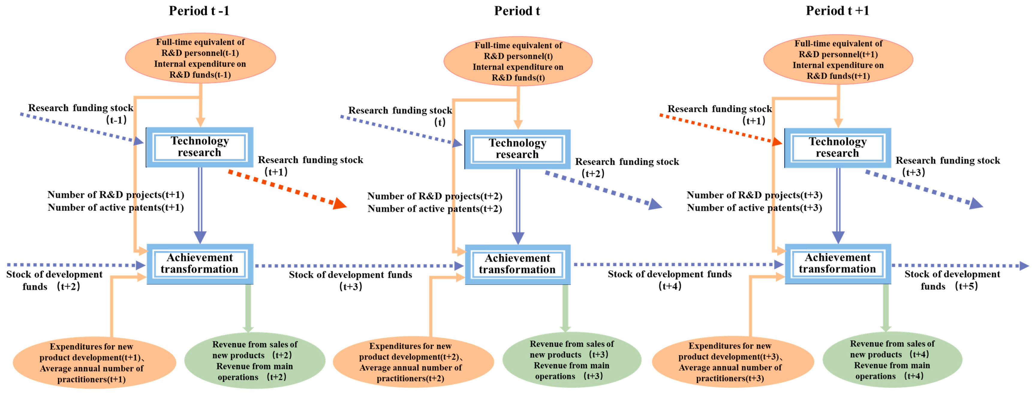
3.1. Selection of the Indicator System

In this paper, the innovation and R&D process of high-tech manufacturing is regarded as a complex two-stage process, in which the first stage is the technology R&D stage, and the second stage is the result transformation stage. The two-stage input structure discussed in this paper includes both shared inputs and independent inputs of each stage. Therefore, when considering the shared inputs, this paper selects the full-time equivalent of R&D personnel as the shared personnel input, and the internal expenditure of R&D funds as the shared capital input; when considering the independent inputs, it selects the expenditure of new product development funds and the annual average number of practitioners as the independent input elements of the result transformation stage. Meanwhile, considering the availability of data, the number of R&D projects and the number of effective invention patents are taken as the linking variables between the technology R&D stage and the result transformation stage, and the sales revenue of new products and the main business revenue are taken as the output variables of the result transformation stage. In addition, referring to the study of Liu, Z.H. et al. [28], the stock of research funding is taken as the carry-over variable of the technology R&D stage, and the stock of development funding is taken as the carry-over variable of the result transformation stage.

Both stages of the innovation process of the high-tech manufacturing industry will have a certain time lag, so in the study of the innovation efficiency of the high-tech manufacturing industry, a certain lag treatment of the corresponding variables needs to be carried out. And there is not yet a unified standard for the lag period of innovation development. Hollanders and Celikel-Esser believe that the use of time lag has almost no effect on the estimation of the innovation efficiency [29]. Preliminary tests were conducted through a series of correlation and regression analyses, which showed that a 2-year lag versus a 1-year lag in the innovation R&D process in the high-tech manufacturing industry had little effect on both innovation efficiency estimates. Therefore, this paper specifies a 2-year lag for the technology R&D stage and a 1-year lag for the result transformation stage.

Based on this, the evaluation indices of innovation and R&D efficiency of the high-tech manufacturing industry, as constructed in this paper, are shown in

Table 1. Evaluation indicators of innovation efficiency of the high-tech manufacturing industry.

Segmentation by Stage	Form	Indicator
Technology research stage	Shared input indicator	Full-time equivalent of R&D personnel (t)
		Internal expenditure on R&D funds (t)
	Link output indicator	Number of R&D projects (t + 2)
		Number of active patents (t + 2)
	Carry-over output indicator	Research funding stock (t + 2)
Achievement transformation stage	Independent input indicator	Expenditures for new product development (t + 2)
		Average annual number of practitioners (t + 2)
	Carry-over output indicator	Stock of development funds (t + 3)
	Final output indicator	Revenue from sales of new products (t + 3)
		Revenue from main operations (t + 3)

.

The dynamic network evaluation structure of two-stage shared inputs for innovative R&D activities in high-tech manufacturing industries is shown in Figure 2.

3.2. Data Sources and Processing

3.2.1. Data Sources

Since the latest data is currently for 2022, some variables have been lagged. Therefore, this paper takes 30 Chinese provinces (Hong Kong, Macao, Taiwan, and Tibet are not included in this study due to data reasons) as the research object in 2016–2019 to analyze the innovation efficiency and change trend of the high-tech manufacturing industry in 30 provinces in China. The original data are from the China Science and Technology Statistical Yearbook (2017–2023) and the China High-Tech Industry Statistical Yearbook (2017 and 2019–2023).

In 2018, officials did not release the Statistical Yearbook of China’s High-Tech Manufacturing Industry; for the missing data related to the high-tech manufacturing industry of individual provinces in 2017, this paper collects and organizes them through the official websites of the regions. For the uncollected data, this paper adopts the linear interpolation method to supplement the missing values (the “annual average number of employees” data of each province in 2017).

3.2.2. Calculation of the Stock of Funds

In this paper, the perpetual inventory method (PIM method) is used to calculate the depreciation of research and development expenditures in the high-tech manufacturing industry in each province to obtain the stock of research expenditures and the stock of development expenditures, respectively.

Research funding stock measurement formula:

$$K_t=\left(1-\delta \right)K_{t-1}+I_{t-2}$$

(11)

where $K_t$ is the stock of research funding in period t, $\delta$ is the rate of depreciation of the stock of research funding, $K_{t-1}$ is the stock of research funding in period t − 1, and $I_{t-2}$ is the constant-price research expenditures, lagged by two periods relative to period t.

The development of a formula for measuring the stock of funds:

$$C_t=\left(1-\delta \right)C_{t-1}+R_{t-1}$$

(12)

where $C_t$ is the stock of development expenditures in period t, $\delta$ is the depreciation rate of the stock of development expenditures, $C_{t-1}$ is the stock of development expenditures in period t − 1, and $R_{t-1}$ is the expenditure of development expenditures at constant prices, lagged by one period relative to period t.

The above formula shows that to estimate the stock of appropriations, it is necessary to know the constant-price appropriation expenditures discounted by the appropriation price index, the rate of depreciation of the stock of appropriations, and the stock of appropriations for the base period.

① Expenditure on constant-price provision

In order to eliminate the effect of data incomparability across periods due to price changes, this paper treats the data with a constant price, and the constant-price treatment uses the provision price index (PI). Drawing on the experience of Deng, J. [30], who set the provision price index as the weighted average of the price index of the personnel labor cost (consumer price index (CPI)), the price index of the daily expenditure on non-personnel labor cost (consumption of raw materials (MPI)) and the price index of investment in fixed assets (IPI), we constructed the price index of provisioning expenditure in China’s high-tech manufacturing industry.

The specific formula for the price index is shown below.

$$PI=a\times CPI+b\times MPI+c\times IPI$$

(13)

According to the China Science and Technology Statistical Yearbook, published by the National Bureau of Statistics, set a = 0.4, b = 0.3, and c = 0.3, thus obtaining the price index of funding expenditures for each year, as shown in

Table 2. Price indices of expenditures.

Particular Year	2015	2016	2017	2018	2019	2020	2021	2022
Expenditure price index	101.03	101.91	107.44	106.28	103.27	101.13	109.48	105.20

.

Thus, it is possible to obtain the annual constant-price expenditure of each province, including constant-price research expenditure and constant-price development expenditure, according to the specific solution formula below.

$$\mathrm{F}\mathrm{i}\mathrm{x}\mathrm{e}\mathrm{d} \mathrm{p}\mathrm{r}\mathrm{i}\mathrm{c}\mathrm{e} \mathrm{e}\mathrm{x}\mathrm{p}\mathrm{e}\mathrm{n}\mathrm{d}\mathrm{i}\mathrm{t}\mathrm{u}\mathrm{r}\mathrm{e}={\displaystyle \frac{\mathrm{e}\mathrm{x}\mathrm{p}\mathrm{e}\mathrm{n}\mathrm{d}\mathrm{i}\mathrm{t}\mathrm{u}\mathrm{r}\mathrm{e}}{\mathrm{E}\mathrm{x}\mathrm{p}\mathrm{e}\mathrm{n}\mathrm{d}\mathrm{i}\mathrm{t}\mathrm{u}\mathrm{r}\mathrm{e} \mathrm{p}\mathrm{r}\mathrm{i}\mathrm{c}\mathrm{e} \mathrm{i}\mathrm{n}\mathrm{d}\mathrm{i}\mathrm{c}\mathrm{e}\mathrm{s}}}$$

② Depreciation rate of provision stock

After analyzing the commonly used methods for determining depreciation rates, Wen Jiaqi suggested assuming the depreciation rate of the fund stock as a fixed value [31]. This article combines the relevant literature and does not consider the impact of changes in the depreciation rate of the funding stock on the calculation of the funding stock. It sets the depreciation rate for both the research funding stock and development funding stock at 15%, that is, $\delta =15\%$.

③ Stock of funds for the base period

It is assumed that the growth rate of the funding stock is equal to the growth rate of funding expenditures:

For measuring the stock of research funding, we have ${\displaystyle \frac{K_t-K_{t-1}}{K_{t-1}}}={\displaystyle \frac{I_t-I_{t-1}}{I_{t-1}}}=h$, which is the average growth rate of I. The stock of research funding in the base period can be calculated as $K_0={\displaystyle \frac{I_0}{h+\delta }}$.

For measuring the stock of development expenditures, we have ${\displaystyle \frac{C_t-C_{t-1}}{C_{t-1}}}={\displaystyle \frac{R_t-R_{t-1}}{R_{t-1}}}=g$, which is the average rate of growth of R. The stock of development funds in the base period can be calculated as $C_0={\displaystyle \frac{R_0}{g+\delta }}$.

Note: Base period funding stock calculations are performed for each province.

3.3. Analysis of Results

To demonstrate the effectiveness of the neutral dynamic network cross-efficiency model, this paper conducts a quantitative, correlational, and non-experimental panel data study. The two-stage resource-sharing model of this paper is compared with the traditional dynamic network model and three cross-efficiency models to evaluate the innovation efficiency of high-tech manufacturing in 30 provinces of China.

3.3.1. Analysis of Cross-Efficiency Modeling Results

First, for the decision-making units without a network structure division, the traditional CCR model was adopted to obtain the annual efficiency values of each decision-making unit. The relevant efficiency results are shown in

Table 3. Efficiency results of traditional CCR model.

Serial Number	DMU	2016	2017	2018	2019	Average Efficiency
1	Shanghai	0.522	0.481	0.352	0.230	0.396
2	Yunnan	0.675	1	0.557	0.466	0.675
3	Neimenggu	0.602	0.346	0.623	1	0.643
4	Beijing	1	1	1	0.569	0.892
5	Jilin	0.396	0.342	0.418	0.761	0.479
6	Sichuan	0.571	0.477	0.479	0.311	0.459
7	Tianjin	0.626	0.681	0.689	0.461	0.614
8	Ningxia	1	1	0.904	1	0.976
9	Anhui	0.927	1	0.790	0.545	0.816
10	Shandong	0.463	0.564	0.695	0.555	0.569
11	Shanxi	0.669	0.631	0.803	0.732	0.709
12	Guangdong	0.948	0.865	0.533	0.347	0.673
13	Guangxi	1	0.645	1	0.565	0.802
14	Xinjiang	1	0.208	1	1	0.802
15	Jiangsu	0.673	0.814	0.615	0.472	0.644
16	Jiangxi	1	1	0.995	0.610	0.901
17	Hebei	0.541	0.573	0.522	0.422	0.514
18	Henan	1	1	1	1	1
19	Zhejiang	0.840	0.903	0.696	0.540	0.745
20	Hainan	0.131	0.119	0.182	0.909	0.335
21	Hubei	0.796	0.728	0.427	0.374	0.581
22	Hunan	0.533	0.568	0.599	0.445	0.536
23	Gansu	1	0.413	0.626	0.348	0.597
24	Fujian	0.756	0.627	0.633	0.335	0.588
25	Guizhou	0.325	0.305	0.329	0.266	0.306
26	Liaoning	0.372	0.351	0.404	0.313	0.360
27	Chongqing	0.979	0.897	0.826	0.447	0.787
28	Shaanxi	0.346	0.255	0.316	0.268	0.296
29	Qinghai	0.705	1	0.949	1	0.913
30	Heilongjiang	0.765	0.492	1	0.337	0.648

.

When observing the results of the CCR model from a vertical perspective of the table, it can be found that there is often more than one decision-making unit with an innovation efficiency value of 1 in each year. Specifically, in 2016, the innovation efficiency value of seven provinces was 1, namely, Beijing, Ningxia, Guangxi, Xinjiang, Jiangxi, Henan, and Gansu. In 2017, it was Yunnan, Beijing, Ningxia, Anhui, Jiangxi, Henan, and Qinghai. In 2018, it was Beijing, Guangxi, Xinjiang, Henan, and Heilongjiang. In 2019, it was Inner Mongolia, Ningxia, Xinjiang, Henan, and Qinghai. The only province that has maintained an innovation efficiency value of 1 for four consecutive years is Henan. Considering the actual situation of various provinces in China, although the comprehensive scientific and technological innovation level of Henan Province has significantly improved, it is not the province with the most outstanding innovation efficiency. This indicates that when the CCR model evaluates the innovation efficiency of high-tech manufacturing industries in various provinces, it may lead to an overestimation of the performance of certain decision-making units and a lack of sufficient discrimination. For this reason, the cross-efficiency model will be adopted for further analysis next.

For the decision-making units without a network structure division, three types of cross-efficiency models were adopted to obtain the annual efficiency values of each decision-making unit. The relevant efficiency results are respectively presented in

Table 4. The benevolent cross-efficiency results.

Serial Number	DMU	2016	2017	2018	2019	Average Efficiency
1	Shanghai	0.461	0.424	0.327	0.192	0.351
2	Yunnan	0.413	0.993	0.469	0.406	0.570
3	Neimenggu	0.246	0.245	0.497	0.723	0.428
4	Beijing	0.857	0.890	1.000	0.382	0.782
5	Jilin	0.348	0.323	0.374	0.391	0.359
6	Sichuan	0.486	0.455	0.450	0.276	0.417
7	Tianjin	0.508	0.559	0.577	0.410	0.514
8	Ningxia	0.967	0.933	0.833	0.923	0.914
9	Anhui	0.827	0.919	0.773	0.462	0.745
10	Shandong	0.391	0.448	0.543	0.495	0.469
11	Shanxi	0.438	0.387	0.690	0.503	0.505
12	Guangdong	0.787	0.766	0.485	0.290	0.582
13	Guangxi	0.428	0.318	0.851	0.265	0.466
14	Xinjiang	0.374	0.109	0.826	0.227	0.384
15	Jiangsu	0.614	0.759	0.609	0.413	0.599
16	Jiangxi	0.901	0.838	0.876	0.544	0.790
17	Hebei	0.446	0.472	0.505	0.313	0.434
18	Henan	0.831	0.802	0.997	0.644	0.819
19	Zhejiang	0.703	0.770	0.656	0.457	0.647
20	Hainan	0.063	0.106	0.175	0.222	0.142
21	Hubei	0.686	0.647	0.398	0.325	0.514
22	Hunan	0.489	0.497	0.589	0.393	0.492
23	Gansu	0.458	0.384	0.532	0.294	0.417
24	Fujian	0.682	0.582	0.544	0.296	0.526
25	Guizhou	0.282	0.294	0.300	0.222	0.275
26	Liaoning	0.334	0.327	0.377	0.270	0.327
27	Chongqing	0.834	0.821	0.787	0.365	0.702
28	Shaanxi	0.297	0.229	0.309	0.230	0.266
29	Qinghai	0.552	0.786	0.701	0.933	0.743
30	Heilongjiang	0.413	0.324	0.717	0.289	0.436

,

Table 5. The adversarial cross-efficiency results.

Serial Number	DMU	2016	2017	2018	2019	Average Efficiency
1	Shanghai	0.396	0.375	0.297	0.168	0.309
2	Yunnan	0.408	0.924	0.409	0.360	0.525
3	Neimenggu	0.269	0.225	0.448	0.739	0.420
4	Beijing	0.742	0.798	0.927	0.333	0.700
5	Jilin	0.304	0.297	0.334	0.412	0.337
6	Sichuan	0.408	0.413	0.414	0.250	0.371
7	Tianjin	0.455	0.522	0.540	0.360	0.469
8	Ningxia	0.886	0.860	0.763	0.833	0.836
9	Anhui	0.715	0.832	0.703	0.400	0.663
10	Shandong	0.345	0.418	0.510	0.434	0.427
11	Shanxi	0.396	0.383	0.640	0.475	0.474
12	Guangdong	0.663	0.673	0.439	0.251	0.506
13	Guangxi	0.424	0.309	0.788	0.277	0.450
14	Xinjiang	0.468	0.109	0.656	0.330	0.391
15	Jiangsu	0.532	0.686	0.556	0.361	0.534
16	Jiangxi	0.780	0.759	0.785	0.487	0.703
17	Hebei	0.400	0.453	0.462	0.294	0.402
18	Henan	0.747	0.762	0.916	0.599	0.756
19	Zhejiang	0.628	0.708	0.595	0.393	0.581
20	Hainan	0.068	0.097	0.157	0.268	0.148
21	Hubei	0.587	0.574	0.369	0.286	0.454
22	Hunan	0.434	0.460	0.538	0.350	0.446
23	Gansu	0.517	0.343	0.481	0.264	0.401
24	Fujian	0.594	0.529	0.505	0.259	0.471
25	Guizhou	0.249	0.270	0.267	0.197	0.246
26	Liaoning	0.289	0.299	0.345	0.237	0.293
27	Chongqing	0.719	0.748	0.722	0.327	0.629
28	Shaanxi	0.265	0.211	0.280	0.200	0.239
29	Qinghai	0.467	0.813	0.687	0.873	0.710
30	Heilongjiang	0.400	0.327	0.636	0.255	0.404

and

Table 6. The neutral cross-efficiency results.

Serial Number	DMU	2016	2017	2018	2019	Average Efficiency
1	Shanghai	0.419	0.399	0.309	0.173	0.325
2	Yunnan	0.401	0.935	0.429	0.368	0.533
3	Neimenggu	0.281	0.238	0.480	0.714	0.428
4	Beijing	0.801	0.848	0.968	0.351	0.742
5	Jilin	0.314	0.306	0.345	0.394	0.340
6	Sichuan	0.432	0.428	0.428	0.257	0.387
7	Tianjin	0.474	0.536	0.562	0.376	0.487
8	Ningxia	0.915	0.899	0.799	0.868	0.870
9	Anhui	0.745	0.865	0.732	0.416	0.689
10	Shandong	0.361	0.433	0.533	0.454	0.445
11	Shanxi	0.390	0.366	0.637	0.475	0.467
12	Guangdong	0.704	0.715	0.457	0.261	0.534
13	Guangxi	0.398	0.305	0.764	0.252	0.430
14	Xinjiang	0.442	0.110	0.737	0.274	0.391
15	Jiangsu	0.551	0.712	0.577	0.376	0.554
16	Jiangxi	0.792	0.785	0.808	0.499	0.721
17	Hebei	0.409	0.457	0.479	0.299	0.411
18	Henan	0.745	0.762	0.932	0.615	0.763
19	Zhejiang	0.650	0.729	0.622	0.412	0.603
20	Hainan	0.069	0.102	0.164	0.262	0.149
21	Hubei	0.624	0.610	0.383	0.298	0.479
22	Hunan	0.447	0.468	0.556	0.358	0.457
23	Gansu	0.512	0.358	0.514	0.270	0.413
24	Fujian	0.624	0.551	0.527	0.271	0.493
25	Guizhou	0.256	0.277	0.279	0.205	0.255
26	Liaoning	0.304	0.307	0.360	0.245	0.304
27	Chongqing	0.743	0.773	0.738	0.336	0.647
28	Shaanxi	0.278	0.220	0.293	0.209	0.250
29	Qinghai	0.484	0.837	0.694	0.861	0.719
30	Heilongjiang	0.399	0.333	0.654	0.263	0.412

.

Overall, from Table 4, Table 5 and Table 6, it can be seen that the three types of cross-efficiency models—benevolent, neutral, and other-suppressing—show significant differences in evaluating the efficiency of each province. The benevolent model has the highest score, followed by the neutral model, and the other-suppressing model has the lowest score. This phenomenon indicates that the three models have different attitudes toward efficiency assessment, and their respective emphasis on evaluation dimensions and tolerance levels also varies.

Meanwhile, in order to better observe the results of the CCR model and the cross-efficiency model, the comparison of the annual efficiency values of the 30 decision-making units using the four models is shown in Figure 3.

As can be seen from Table 3, Table 4, Table 5 and Table 6 and Figure 3, for each decision unit, the cross-efficiency values of the three types are generally lower than those in the traditional CCR model. In the CCR model, there is usually more than one decision unit with an efficiency value of 1, which may lead to overestimation of the performance of certain decision units and a lack of differentiation. The three-category cross-efficiency model, on the other hand, can provide a more detailed and comprehensive evaluation and ranking of all the provinces, avoiding the situation where the efficiency value is too concentrated at 1, thus improving the differentiation and usefulness of the model. Meanwhile, among the three types of cross-efficiency values, the neutral cross-efficiency value is usually located between the benevolent cross-efficiency value and the adversarial cross-efficiency value, which indicates that the neutral model neither favors any party nor overly oppresses the other decision-making units in its evaluation of decision-making units, thus presenting a relatively balanced evaluation method. Compared with the benevolent and adversarial models, the neutral cross-efficiency model is more suitable for evaluating those decision-making units that need to consider the cooperation and game relationship in a comprehensive way, in which it can more accurately reflect the actual efficiency of each decision-making unit in interaction and competition.

3.3.2. Analysis of the Results of the Two-Stage Dynamic Network Model

Using the two-stage dynamic network model in Section 2.2 to assess the 30 provinces, it is able to obtain the overall efficiency value, the stage-one efficiency value, and the stage-two efficiency value (

Table 7. Overall efficiency results of the two-stage dynamic network.

Serial Number	DMU	Overall Efficiency Value	Stage 1 Efficiency Value	Stage 2 Efficiency Value
1	Shanghai	0.774405	0.443462	0.146154
2	Yunnan	0.947053	0.332505	0.448106
3	Neimenggu	0.863417	0.495243	0.325395
4	Beijing	1	0.590699	0.612533
5	Jilin	0.758956	0.446096	0.200793
6	Sichuan	0.802218	0.486668	0.279002
7	Tianjin	0.928797	0.302415	0.429519
8	Ningxia	1	0.318312	0.753214
9	Anhui	0.990402	0.604228	0.487683
10	Shandong	0.921920	0.364952	0.418672
11	Shanxi	1	0.168742	0.548059
12	Guangdong	0.856469	0.570199	0.053439
13	Guangxi	0.975229	0.606961	0.467347
14	Xinjiang	0.764179	0.510609	0.146037
15	Jiangsu	0.931260	0.393364	0.422927
16	Jiangxi	1	0.441619	0.547284
17	Hebei	0.866948	0.308851	0.366886
18	Henan	1	0.274016	0.910339
19	Zhejiang	0.959041	0.383756	0.456063
20	Hainan	0.682115	0.438424	0.048969
21	Hubei	0.847507	0.581689	0.204838
22	Hunan	0.878838	0.360040	0.377812
23	Gansu	0.783275	0.281361	0.283223
24	Fujian	0.875199	0.384368	0.372973
25	Guizhou	0.728923	0.405509	0.161186
26	Liaoning	0.747690	0.406133	0.230784
27	Chongqing	1.000000	0.420755	0.537713
28	Shaanxi	0.696487	0.233117	0.193475
29	Qinghai	1	0.628615	0.728512
30	Heilongjiang	0.845018	0.243439	0.345608

). The model takes into account the two-stage relationship of the technological innovation process in China’s high-tech manufacturing industry and introduces a time dimension, which makes the assessment of the innovation efficiency of each province more comprehensive and dynamic. By dividing the innovation process into two stages: technology development and achievement transformation and setting different lags in the model, the efficiency differences between the stages can be visualized. This design enables the model to reveal more precisely the innovation performance of each stage at different points in time, helping to analyze the bottlenecks and potential advantages of a particular stage within a certain time period. In addition, the introduction of the time dimension helps to better grasp the lag effect of innovation activities, thus providing more specific decision support for policymakers and promoting the positive interaction between technological innovation and achievement transformation.

According to Table 7, it can be seen that about half of the provinces are more efficient at the technology R&D stage than at the transformation stage. This suggests that in these provinces, the input and output efficiencies of innovative technology R&D are more prominent, while there may be certain bottlenecks or inefficiencies in the transformation stage, resulting in a relatively weaker ability to transform their results. However, although the dynamic network DEA model has improved over the traditional self-assessment model in some aspects, it still retains some of the limitations of the traditional DEA model, especially in assessing efficient decision-making units. Specifically, a number of provinces, including Beijing, Ningxia, Shanxi, Jiangxi, Henan, Chongqing, and Qinghai, have an overall efficiency value of 1 and are assessed as “optimally efficient” units in the model; the reason might be that the model failed to fully identify their potential inefficiency problems during the evaluation process. This suggests that the efficiency results for these provinces may not be scientifically sound and that the model may need to be further optimized in order to reveal the relative efficiency differences and potential problems of the provinces at different stages more accurately.

Qinghai Province has demonstrated the highest efficiency in the stage of technological research and development. The reasons mainly lie in its unique resource advantages; the promotion of industrial upgrading by scientific and technological innovation, ecological restoration, and sustainable development; the transformation of the innovation system and mechanism; as well as modern agricultural innovation. At the same time, the efficiency of its technology transfer stage is also relatively high, with an overall efficiency of 1. It can be temporarily considered that the result is in line with the factual basis. However, Henan Province has a relatively complete industrial chain and a good infrastructure and has also increased investment in innovation and technology, promoting cooperation between enterprises and research institutions. It shows the highest efficiency in the stage of technology transfer, but its efficiency in the research and development stage is relatively low. Nevertheless, the overall efficiency is still 1, which can also indicate that this model still overestimates the evaluation results.

The following takes Hebei Province as an example to analyze its overall efficiency, stage-one efficiency, and stage-two efficiency in the two-stage dynamic network model, as shown in

Table 8. Overall efficiency results for Hebei Province in the two-stage dynamic network model.

Hebei	Overall Efficiency Value	Stage 1 Efficiency Value	Stage 2 Efficiency Value
Full cycle	0.866948	0.308851	0.366886
2016	0.334131	0.155995	0.337072
2017	0.433745	0.315810	0.435771
2018	0.373970	0.369668	0.374011
2019	0.334313	0.450185	0.333258

and Figure 4. From the data, it can be seen that with the continuous development of the high-tech manufacturing industry in Hebei Province, the efficiency of the technology R&D stage (stage one) has been on an upward trend year by year, showing certain positive changes. This trend indicates that Hebei Province has gradually achieved results in technological innovation and R&D investment, especially in the construction of scientific research and technological infrastructure. However, it is worth noting that the overall efficiency of the high-tech manufacturing industry in Hebei Province is as high as 0.866948 over the entire assessment cycle, which means that Hebei Province has demonstrated high overall efficiency in the overall dimension over the entire assessment period. However, further analysis reveals that the overall efficiency in each year does not exceed 0.5, a phenomenon that highlights certain limitations of the dynamic network DEA in dealing with efficiency evaluation. Meanwhile, when breaking down the overall efficiency of each stage, it is found that the overall efficiency of stage one is only 0.308851, and the efficiency of stage two is 0.366886, and the efficiencies of the two stages are not up to the ideal level, which indicates that Hebei Province is still facing a lot of bottlenecks in the innovation chain of the high-tech manufacturing industry.

3.3.3. Analysis of the Results of the Two-Stage Dynamic Network Cross-Efficiency Model

The dynamic network cross-efficiency model with two stages of resource sharing proposed in this paper is used to assess the innovation efficiency of the high-tech manufacturing industry in 30 provinces in China, and the calculation results are shown in

Table 9. Overall dynamic network cross-efficiency results for both phases.

Serial Number	DMU	Overall Efficiency Value	Stage 1 Efficiency Value	Stage 2 Efficiency Value
1	Shanghai	0.813357	0.249872	0.824476
2	Yunnan	0.810733	0.253328	0.820066
3	Neimenggu	0.811440	0.234682	0.823061
4	Beijing	0.801637	0.548428	0.812584
5	Jilin	0.813297	0.409206	0.816844
6	Sichuan	0.812225	0.253072	0.821677
7	Tianjin	0.808339	0.268955	0.816890
8	Ningxia	0.796537	0.219304	0.807736
9	Anhui	0.799821	0.235918	0.809517
10	Shandong	0.808562	0.270846	0.817088
11	Shanxi	0.813070	0.235249	0.822682
12	Guangdong	0.807938	0.251826	0.819104
13	Guangxi	0.816251	0.243628	0.826848
14	Xinjiang	0.821312	0.330308	0.821530
15	Jiangsu	0.808527	0.254284	0.818083
16	Jiangxi	0.809149	0.229838	0.820081
17	Hebei	0.807175	0.263308	0.808980
18	Henan	0.805053	0.225447	0.808061
19	Zhejiang	0.799889	0.241973	0.809114
20	Hainan	0.834021	0.324571	0.842910
21	Hubei	0.808363	0.251950	0.819425
22	Hunan	0.810506	0.255088	0.819720
23	Gansu	0.810213	0.250349	0.819847
24	Fujian	0.808588	0.254699	0.817627
25	Guizhou	0.816073	0.426705	0.817243
26	Liaoning	0.813300	0.255949	0.822585
27	Chongqing	0.809759	0.228837	0.819621
28	Shaanxi	0.812482	0.278667	0.820348
29	Qinghai	0.806722	0.225267	0.815790
30	Heilongjiang	0.806412	0.288813	0.806941

.

According to the results in Table 9, it can be seen that all 30 provinces have different efficiencies in various categories throughout the assessment cycle, which makes it easier to rank them, and all the efficiencies in various categories show an upward trend. This trend indicates that the efficiency of Chinese provinces has been continuously improved in the development process of the high-tech manufacturing industry. Whether in the process of technology R&D or in the process of transformation of achievements, the industrial efficiency has made significant progress. Guizhou Province had the highest efficiency value in the first stage, specifically, 0.426705, indicating that it has an advantage in research and development. Although the overall efficiency is moderate, it has a disadvantage in commercialization. Hainan Province had the highest efficiency value in the second stage, reaching 0.842910, and its efficiency value in the first stage was also relatively high, with the overall efficiency being the highest.

Meanwhile, the efficiency of most provinces in the technology R&D stage is generally lower than that in the transformation stage of their achievements. This phenomenon reveals the overall development characteristics of China’s high-tech manufacturing industry, i.e., more resources and efforts are focused on the transformation and commercialization of technological achievements, demonstrating strong product marketability, while efficiency improvement at the technology R&D stage is relatively lagging behind. This may be closely related to some limitations of China’s domestic technological innovation system. In the early stage of technological research and development, the return cycle of R&D investment is longer, and technological breakthroughs have a high degree of uncertainty; in the middle and late stages of R&D, there may be some constraints or “neck-breaking” problems, which require the strengthening of basic research, technological accumulation, and the improvement of the innovation system.

The following takes Hebei Province as an example to analyze its overall efficiency, the efficiency of stage one, and the efficiency of stage two in the two-stage dynamic network cross-efficiency model, as shown in

Table 10. Overall efficiency results for Hebei Province in the two-stage dynamic network cross-efficiency model.

Hebei	Overall Efficiency Value	Stage 1 Efficiency Value	Stage 2 Efficiency Value
Full cycle	0.807175	0.263308	0.808980
2016	0.602637	0.213525	0.603283
2017	0.723661	0.460353	0.724044
2018	0.724006	0.445400	0.724327
2019	0.620914	0.396470	0.621245

and Figure 5. By comparing Figure 5 and Figure 4, it can be found that in the two models, the overall efficiency of innovation activities in the high-tech manufacturing industry in Hebei Province and the efficiency of stage two show a similar trend; while stage one in the dynamic network model shows a rising trend year by year, the efficiency of stage one in the dynamic network cross-efficiency model increases rapidly in the first year, and then the efficiency of the following two years shows a slight decline. This trend of change is closer to the actual development of Hebei Province. Despite the outbreak of the global pneumonia epidemic in 2019, which caused most enterprises and research institutions to enter the home office mode, and production activities were affected to varying degrees, innovative technology research and development activities were able to ensure that they basically continued, which explains to a certain extent the insignificant decrease in stage-one efficiency. The declines in the overall efficiency and stage-two efficiency were relatively large.

Through modeling, the overall cross-efficiency value of Hebei Province was finally assessed to be 0.807175; the cross-efficiency value of stage one, to be 0.263308; and the cross-efficiency value of stage two, to be 0.808980, and these efficiency values are relatively reasonable. The efficiency of the technology R&D stage is related to the long-term and complexity of technological innovation as well as the input and output of R&D resources, and although the efficiency of this stage is low, this inefficiency does not mean ineffectiveness. Therefore, it can be considered that the two-stage dynamic network cross-efficiency model proposed in this paper is feasible to be applied in the high-tech manufacturing industry in Chinese provinces and has higher scientificity and rationality than the traditional DEA model. The model can better reflect the complex innovation chain of the high-tech manufacturing industry, especially under the influences of multiple stages and multiple factors, and it can more accurately assess the efficiency performances of different stages and provide a more powerful basis for related policymaking.

4. Discussion

This paper proposes a neutral dynamic network cross-efficiency model and applies it to the assessment of the efficiency of innovation activities in China’s high-tech manufacturing industry. This paper divides the innovation activities of China’s high-tech manufacturing industry into the technology R&D stage and the achievement transformation stage. In order to reflect the actual delay effect of technology R&D and achievement transformation more accurately, this paper lags the technology R&D stage by 2 years and the achievement transformation stage by 1 year and utilizes the model to comprehensively assess the overall efficiency of China’s provincial-level high-tech manufacturing industry as well as the efficiency of each stage. The assessment results show that the overall efficiency performance of China’s high-tech manufacturing industry is relatively excellent. The overall efficiency values of all the evaluated provinces are generally close to 0.8, indicating that most provinces have achieved relatively ideal results in the overall operation of high-tech manufacturing. However, upon in-depth analysis of the efficiency at each stage, it was found that the average efficiency of the technology transfer stage was as high as 0.818216 but that of the technology research and development stage was 0.275346. This indicates that although China has made certain progress in promoting the development of high-tech manufacturing, there is still room for efficiency improvement in the field of technological research and development, and it is necessary to continuously strengthen basic research and technological accumulation. In order to realize the dual-wheel drive of technology R&D and achievement transformation, it is still necessary to invest more attention and resources in the technology R&D stage, to enhance R&D capabilities and break down technological barriers, and to promote the overall optimization from the source of the technology to its market application. This will not only help to improve the overall level of technological innovation but also win a greater advantage for China’s high-tech manufacturing industry in global competition.

Based on the above conclusions, combined with the development status of China’s high-tech manufacturing industry, the following suggestions are given:

(1) The government and enterprises have increased their investment in technological research and development, especially in basic research and the development of key core technologies, to ensure the effective allocation and utilization of research and development resources. Support for scientific researchers should be strengthened, the cultivation and introduction of high-end scientific research talents should be encouraged, and enterprises should be encouraged to increase their R&D expenditures through policy guidance to enhance their overall technology R&D capabilities;

(2) The connection mechanism between technology R&D and achievement transformation should be optimized, and the lag effect between technology R&D and achievement transformation should be shortened. It is suggested that the smooth transition of technological achievements from the laboratory to the market can be promoted through the establishment of industry–university–research combination platforms, innovation incubators, and technology transfer centers, so as to enhance the conversion rate of achievements;

(3) In view of the differences in the industrial foundation, resource endowment, and development stages of different provinces, the government should formulate differentiated development strategies based on the characteristics and advantages of each region. Through cross-regional technical cooperation and resource sharing, it should promote inter-regional collaborative innovation and enhance the overall innovation and development level of the national high-tech manufacturing industry.

References

1. Zhang, X.Y.; Zheng, X.R.; Li, S.Q.; Wei, A.L. Measurement of the Development Level of China’s Provincial High-Tech Industries from 2019 to 2021. Stat. Appl. 2024, 13, 202–219. [Google Scholar]
2. Han, C.; Thomas, S.R.; Yang, M.; Ieromonachou, P.; Zhang, H.R. Evaluating R&D investment efficiency in China’s high-tech industry. J. High Technol. Manag. Res. 2017, 28, 93–109. [Google Scholar]
3. Ding, S. A novel discrete grey multivariable model and its application in forecasting the output value of China’s high-tech industries. Comput. Ind. Eng. 2019, 127, 749–760. [Google Scholar] [CrossRef]
4. Li, J.; Feng, H.Y. The Economic Growth Effect of the High-tech Manufacturing Industry and High-Tech Service Industry Co-Agglomeration. Sci. Technol. Prog. Policy 2020, 37, 54–62. [Google Scholar]
5. Yu, K.; Gong, R.; Hu, S.; Luo, Y. Based on Analytic Hierarchy Process to Discuss Key Factors in High-tech Industrial Ecology Development. Ekoloji Derg. 2018, 106, 449. [Google Scholar]
6. Meng, L.; Sun, L.Y. The Influencing Factors of Technological Innovation Efficiency in High-tech Industry: An Analysis from the Perspective of Industry. J. Nanchang Norm. Univ. 2019, 40, 20–22. [Google Scholar]
7. Gui, J.Y. Measurement and Improvement Strategy of China’s Provincial High-tech Industry Development Level. Econ. Rev. J. 2018, 7, 83–92. [Google Scholar]
8. Chen, X.X.; Shi, D.H. An Analysis of the Comprehensive Evaluation of High-Quality Development of High-tech Industry in China. J. Nanjing Univ. Financ. Econ. 2019, 5, 34–44. [Google Scholar]
9. Wang, Z.X.; Wang, Y.Y. Evaluation of the provincial competitiveness of the Chinese high-tech industry using an improved TOPSIS method. Expert Syst. Appl. 2014, 41, 2824–2831. [Google Scholar] [CrossRef]
10. Wang, R.D.; Zhang, J.J. Research on the measurement of the level of global industrial chain of China’s provincial high tech industry. Times Econ. Trade 2020, 29, 6–10. [Google Scholar]
11. Liu, C.Y.; Gao, X.Y.; Ma, W.L.; Chen, X.T. Research on regional differences and influencing factors of green technology innovation efficiency of China’s high-tech industry. J. Comput. Appl. Math. 2020, 369, 112597. [Google Scholar] [CrossRef]
12. Yang, X.Q.; Peng, J.X.; Wang, J. Research on the Transformation Efficiency of Scientific and Technological Achievements of High-tech Industry in China Based on DEA Model. Inn. Mong. Sci. Technol. Econ. 2023, 12, 25–27. [Google Scholar]
13. Zhang, B.; Luo, Y.; Chiu, Y.H. Efficiency evaluation of China’s high-tech industry with a multi-activity network data envelopment analysis approach. Socio-Econ. Plan. Sci. 2019, 66, 2–9. [Google Scholar] [CrossRef]
14. Yu, Y.; Liao, J.Q.; Wang, X.M.; Zhu, W.W. Identifying the drivers of new product development performance change in China’s high-tech industry: A two-stage production-theoretical decomposition analysis. Expert Syst. Appl. 2024, 261, 125513. [Google Scholar] [CrossRef]
15. Yang, J.W.; Wang, M.Q.; Li, D. Research on R&D Innovation Efficiency Evaluation of China’s Provincial High-tech Industry Based on Two-stage DEA Model with Shared Inputs. Sci. Technol. Manag. Res. 2017, 37, 84–90. [Google Scholar]
16. Wang, Y.; Pan, J.F.; Pei, R.M.; Yi, B.W.; Yang, G.L. Assessing the technological innovation efficiency of China’s high-tech industries with a two-stage network DEA approach. Socio-Econ. Plan. Sci. 2020, 71, 100810. [Google Scholar] [CrossRef]
17. Chen, Y.W.; Wang, M.Q.; Chen, Y.Y.; Geng, J.G. Research on the Efficiency of China’s High-tech Industry R&D Innovation Based on the Improved Two-stage DEA. Soft Sci. 2018, 32, 14–18. [Google Scholar]
18. Lin, S.F.; Lin, R.Y.; Sun, J.; Wang, F.; Wu, W.X. Dynamically evaluating technological innovation efficiency of high-tech industry in China: Provincial, regional and industrial perspective. Socio-Econ. Plan. Sci. 2021, 74, 100939. [Google Scholar] [CrossRef]
19. Chen, W.; Zhang, C.X.; Li, C.Y.; Feng, Z.J. Innovation Efficiency Evaluation of New and High Technology Industries Based on DEA-Malmquist Index. Sci. Technol. Manag. Res. 2017, 37, 79–84. [Google Scholar] [CrossRef]
20. Wang, S.T.; Lin, X. Research on innovation efficiency evaluation of high-tech enterprises based on DEA-Malmquist index model. Hebei Enterp. 2024, 9, 21–25. [Google Scholar]
21. He, Y.B.; Zhang, S.; Lin, T. Research on efficiency measurement of China’s high-tech industry innovation ecosystem and its improvement path. Syst. Eng.—Theory Pract. 2024, 44, 546–562. [Google Scholar]
22. Wang, Q.J.; Wang, Q.; Zhou, X. Research on Efficiency Evaluation and Influencing Factors of High-Tech Industry R&D Activities. Sci. Technol. Prog. Policy 2018, 35, 59–65. [Google Scholar]
23. Sexton, T.R.; Silkman, R.H.; Hogan, A.J. Data envelopment analysis: Critique and extensions. New Dir. Program Eval. 1986, 32, 73–105. [Google Scholar] [CrossRef]
24. Doyle, J.; Green, R. Efficiency and cross efficiency in DEA: Derivations meanings and the uses. J. Oper. Res. Soc. 1994, 45, 567–578. [Google Scholar] [CrossRef]
25. Wang, Y.M.; Chin, K.S. A neutral DEA model for cross—Efficiency evaluation and its extension. Expert Syst. Appl. 2010, 37, 3666–3675. [Google Scholar] [CrossRef]
26. Charnes, A.; Cooper, W.W. Management, Model and Industrial Applications of Linear Programming; Wiley: New York, NY, USA, 1962. [Google Scholar]
27. Chen, Y.; Du, J.; Sherman, H.D.; Zhu, J. DEA model with shared resources and efficiency decomposition. Eur. J. Oper. Res. 2010, 207, 339–349. [Google Scholar] [CrossRef]
28. Liu, Z.H.; Xi, C.J.; Yang, Y. The Measurement Method of Regional Scientific and Technological Innovation Efficiency Based on Dynamic Network SBM Model. Inf. Sci. 2022, 40, 145–153. [Google Scholar]
29. Hollanders, H.J.; Celikel-Esser, F. Measuring Innovation Efficiency; INNO Metrics Thematic Paper; European Commission: Brussels, Belgium, 2007. [Google Scholar]
30. Deng, J. The R&D Capital Stock and Output Efficiency of the Hi-tech Industry in China. South China J. Econ. 2007, 8, 56–64. [Google Scholar]
31. Wen, J.Q. Research on the measurement of enterprise R&D capital stock under the perspective of SNA. China Collect. Econ. 2022, 31, 91–93. [Google Scholar]
Figure 1. Mathematical structure of two-stage dynamic network model.
Applsci 15 08552 g001
Figure 2. Structure of innovative R&D activities in the high-tech manufacturing industry.
Applsci 15 08552 g002
Figure 3. Annual efficiency comparison according to four DEA models.
Applsci 15 08552 g003
Figure 4. Efficiency values of various categories in Hebei Province in dynamic network modeling.
Applsci 15 08552 g004
Figure 5. Various efficiency values of Hebei Province in the dynamic network cross-efficiency model.
Applsci 15 08552 g005