A Stress Analysis of a Thin-Walled, Open-Section, Beam Structure: The Combined Flexural Shear, Bending and Torsion of a Cantilever Channel Beam

Abstract

Channels with three standard symmetrical sections and one asymmetric section are mounted as cantilever beams with the web oriented vertically. A classical solution to the analysis of stress in each thin-walled cantilever channel is provided using the principle of wall shear flow superposition. The latter is coupled with a further superposition between axial stress arising from bending and from the constraint placed on free warping imposed at the fixed end. Closed solutions for design are tabulated for the net shear stress and the net axial stress at points around any section within the length. Stress distributions thus derived serve as a benchmark structure for alternative numerical solutions and for experimental investigations. The conversion of the transverse free end-loading applied to a thin-walled cantilever channel into the shear and axial stress that it must bear is outlined. It is shown that the point at which this loading is applied within the cross-section is crucial to this stress conversion. When a single force is applied to an arbitrary point at the free-end section, three loading effects arise generally: bending, flexural shear and torsion. The analysis of each effect requires that this force’s components are resolved to align with the section’s principal axes. These forces are then considered in reference to its centroid and to its shear centre. This shows that axial stress arises directly from bending and from the constraint imposed on free warping at the fixed end. Shear stress arises from flexural shear and also from torsion with a load offset from the shear centre. When the three actions are combined, the net stresses of each action are considered within the ability of the structure to resist collapse from plasticity and buckling. The novelty herein refers to the presentation of the shear flow calculations within a thin wall as they arise from an end load offset from the shear centre. It is shown how the principle of superposition can be applied to individual shear flow and axial stress distributions arising from flexural bending, shear and torsion. Therein, the new concept of a ‘trans-moment’ appears from the transfer in moments from their axes through centroid G to parallel axes through shear centre E. The trans-moment complements the static equilibrium condition, in which a shift in transverse force components from G to E is accompanied by torsion and bending about the flexural axis through E.

1. Introduction

This paper extends the thin-walled beam theory outlined and derived previously using the geometry of three extruded aluminium alloy channels to US specification [1]. Therein, the point was emphasised that each thin-walled beam structure requires individual consideration depending upon the cross-section and the manner of its support under an imposed loading. What might appear as a simple structure is deceiving from the complex analyses required of its stress state and consequently the likely mode of its failure. It is a testimony to classical elasticity theory that solutions are forthcoming from its linear constitutive relation, coupled with a description of force and torque equilibrium, with strain and displacement compatibility matched to the boundary conditions that prevail. This theory has long been applied by the Engineering Science Data Unit (ESDU) in the UK to develop a library of case studies of lightweight alloy beam structures used in applications where the weight to strength ratio is an issue. Their data sheets have been produced on a variety of related topics including plate buckling within thin I, Z and U sections [2]. The present work has been undertaken to provide further useful design data in this arena. In particular, given the prevalence of the FEM today for stress analysis, these design data can be configured for the validation of an FE stress analysis. A theoretical approach can serve to validate finite element predictions and also provide the benchmark for comparisons with experimental data found from scaled model testing. The present approach adopts the classical theory where it is able provide closed solutions for a specific structure. Fortunately, here, there are many practical applications of thin structures to which the theory can be applied, especially those where minimum weight restrictions are imposed. More recent developments with thin structures include thin-film technology [3] and flexible devices [4]. It is expected that a thin-walled stress analysis would have relevance here in the presence of mechanical loading involving twist, stretch and bend in static and dynamic applications.

Previously, in Ref. [1], the flexural shear, bending and torsion of a thin-walled cantilever beam of an open cross-section were derived and considered separately. For an open channel section, with x-axis symmetry, the axes of loading were referred to shear centre E, centroid G and another arbitrary position, O, at the centre of the web. In the case of an axial torsion, it was shown how both the free-end and constrained-end warping displacements depended upon the axis of torsion coincident with the stated positions. So too does the axial stress depend upon the torsion axis as it is induced by the fixed-end constraint. It was seen that beam flexure involving bending and shear act together only when transverse point forces act upon the shear centre. In this paper, bending moments accompanying transverse forces may be displaced from x and y axes at G to parallel axes at E after applying bending theory. It is shown here that any the shift between said axes also involves a trans-moment, but this moment does not arise when E and G lie upon a common x-axis for an axially symmetric channel section. Stress analysis considers the torsion, shear and bending that arise when transverse forces applied at G are displaced to shear centre E. The common centre enables a superposition between similar stress from different sources. A net shear flow is found as a sum of the flows from shear and torsion arising from the applied transverse forces. Accompanying this, a net axial stress also arises as a sum of the axial stress from bending and from the beam’s end constraint. The latter induces axial stress by preventing the axial warping displacement that would otherwise occur under torsion when the ends are free. The safety of the beam against plastic collapse and buckling failure must consider both net shear and axial stresses, say, within criteria of yielding, applied to where each stress is at its most severe. Other work has been reported by Papangelis [5] on the stresses in thin-walled channel structures under torsion. With axial torsion applied specifically, the local buckling of the channel walls is confined to the most highly stressed constrained regions, say within the web at an end fixing. In unconstrained torsion, global torsional buckling is most likely to happen by allowing warping to occur freely. However, where any constraint to free warping arises from clamping ends and sides, the clamping also introduces additional axial stress that is quantified herein. This stress arises despite no external axial force being applied in these studies. Vibratory axial loading was applied in combination with torsion in the work of Yu et al. [6]. Again, when the torsion is constrained, then axial stress is imposed upon cyclic applications of this stress to introduce a further risk of fatigue failure. Complex modes of failure can arise where gross yielding and buckling, both local and global, are coupled with fatigue. When an endurance estimate proves intractable, then testing would be recommended. There follows an analysis here of the torsion arising from transverse forces applied to the centroid at the free end of a cantilever channel. The stress state is again complex but different from those cited in that said forces also bend and shear the channel over its length.

Thin-Walled Elasticity Theory

In a minor departure from the original Vlasov theory [7,8], the co-ordinates z in this paper refers to length and x and y to the section’s centroid as an origin. The general equations to be applied in this work refer to the two thin-walled sections of a cantilever beam shown in Figure 1a,b. In the x-symmetric section of Figure 1a transverse horizontal and vertical forces, F_x and F_y, respectively, are applied at centroid G of a thin-walled cantilever beam in which x and y are centroidal axes at G (see Figure 1a). When F_x and F_y are applied at shear centre E as shown, then the section is subjected to transverse shear and bending without torsion. Loading at point E in free space may not be achieved easily in practice. Usually the forces are referred to the section’s centroid at G. Then, with transverse forces displaced from shear centre E to centroid G, the bending, shear and torsion of the beam arises [9]. A corollary applies that when pure axial torsion applied at E twists and does not bend the cross-section. Point E is then referred to as the centre of twist, i.e., the point in the section that does not rotate. Therefore, pure axial torsion is applied to longitudinal axis z through shear centre E [10,11]. Similar features apply to E and G for the thin-walled non-symmetric section shown in Figure 1b, provided axes u and v replace x and y as the section’s principal centroidal axes. Here, the axial stress due to bending is applied to the thin section’s principal axes u and v. Axes u and v will coincide with x and y, with x as a symmetry axis for standard channel sections mounted with a vertical web and equal flange lengths. However, if the applied transverse forces are displaced from G to any arbitrary point, O, in the cross-section, then a transformation is required between in-plane axes at E, G and O for the bending, torsion and transverse shear stress calculations under each of these three actions. In Ref. [1], it was shown how to calculate net axial stress and the net shear stress for this condition when O lies at the centre of the vertical web for each of the three symmetrical channel cantilever beams. In this paper, with all loading applied at G, these transformations are restricted to apply between G and E.

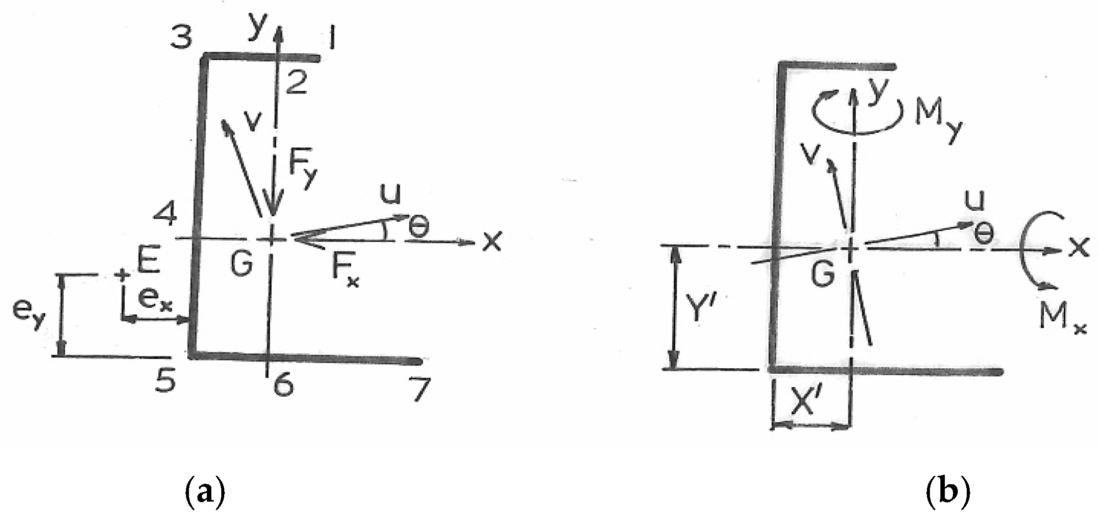
2. Non-Symmetric Cross-Section

In its most general form, the Vlasov theory [7,8] applies to any thin-walled, non-symmetric, open cross-section (see Figure 1a,b). The theory is limited to small deformation linear elasticity in which infinitesimal strain is compatible with the first derivative of displacement. Forces applied are in static equilibrium with internal stress distributions, and the boundary conditions are matched to each thin-walled structure. Here, a cantilever beam with different thin-walled channel sections is examined. Stress analyses are presented for three symmetrical sections of standard US dimensions and one non-symmetrical channel with unequal flange lengths. Transverse forces F_x and F_y are applied at the centroid of the free-end section.

2.1. Bending

Bending moments should be referred to equivalent moments M_x’ and M_y’ that are applied to the section’s principal centroidal axes u and v [12,13,14]. These moments appear with the centroid’s reference co-ordinates x and y to give the axial bending stress as follows:

σ_z = M_x’y/I_x + M_y’/I_y

(1a)

M_x’ = [M_x − M_y (I_xy/I_y)]∍[1 − I_xy²/(I_x I_y)]

(1b)

M_y’ = [M_y − M_x (I_xy/I_x)]∍[1 − I_xy²/(I_x I_y)]

(1c)

in which I_x, I_y and I_xy are the second moments of area for the cross-section for its reference axes x and y. Equations (1a–c) are convenient forms that do not require the calculation of the principal values I_u and I_v and their orientations with respect to x and y.

2.2. Shear

Let both vertical F_y and horizontal F_x shear forces be applied to shear centre E in the negative x and y directions (see Figure 1a,b). For a non-symmetric section, flexural shear under each transverse force must apply to shear centre axes aligned with principal directions u and v.

The shear flow distribution, q = τt, around the section’s mean wall perimeter dimension, s, can be derived from [1]

q = (F_x’/I_y) D_y + (F_y’/I_x) D_x

(2a)

where F_x’ and F_y’ are equivalent forces applied to principal axes u and v. Given F_x = dM_y/dz and F_y = dM_x/dz, each derivative is applied to Equation (1b,c) to provide the following equivalent shear forces [15], appearing in Equation (2a):

F_x’ = [F_x − F_y (I_xy/I_x)] ∍ [1 − I_xy²/(I_x I_y)]

(2b)

F_y’ = [F_y − F_x (I_xy/I_y)] ∍ [1 − I_xy²/(I_x I_y)]

(2c)

D_x and D_y in Equation (2a) are the running first moments of area integrals about axes x and y for the wall area with an origin for s at a free surface. The two integrals are D_x = ∫_A y dA and D_y = ∫_A dA for dA = t ds. In the case of a symmetric channel section about the x-axis (see Figure 1a), then I_xy = 0, thus giving F_x’ = F_x and F_y’ = F_y in Equation (2a).

2.3. Axial Stress Superposition

When both ends of the beam are free, the unconstrained warping displacements, w_o, can be found from St Venant’s torsion theory [9,10,11]. Therein, points in a plane cross-section are free to displace axially (warp) with the distortion of that plane arising from torsion, i.e., plane cross-sections do not remain plane. With one end encastre (fixed), a full constraint applies to the fixing where no warping occurs. Elsewhere along the length of a cantilever, the constraint to free warping extends to a lesser degree. Consequently, axial stress is induced in all but the free end beam section, i.e., for 0 # z < L. This stress is proportional to w_o but is non-linear (hyperbolic) in z. Here, the net axial stress arising from constrained warping is added to Equation (1a) [1]:

σ_z = μEw_o{sinh [μ(L − z)] ∍ cosh (μL)} σ_z + M_x’y/I_x + M_y’x/I_y

(3a)

where w_o is the unconstrained warping displacement, μ = √(GJ/EΓ₁) in which Γ₁ = ${\int }_0^s($2A_E) t ds is the primary warping constant. This gives

w_o = −(2A_E)T ∍ (GJ) = −(ꞷ − ϖ)T ∍ (GJ)

(3b)

where A_E = (ꞷ−ϖ)/2 is the ‘swept area’ of the section between E and each perimeter point (see Figure 2). Equation (3a,b) enable the net axial stress to be evaluated separately from the net shear stress, as will follow. Geometrically, it will be seen that axial stress distributions within a thin-walled, open-section cantilever beam, arising from each source, may be overlaid to provide a net axial stress distribution for the cross-section at any given length position, z.

2.4. Net Shear Stress

The shear stress due to transverse shear and axial torsion is to be investigated here. A torsional shear flow analysis requires that a longitudinal axis passing through E in Figure 1b receives a net torque:

T = F_y e_x − F_x e_y

(4)

where e_x and e_y are the perpendicular distances from F_y and F_x to E, as shown in Figure 1b.

Note (1): For the axially symmetric channels considered here, with a vertical web and horizontal flanges, the line of action of F_x passes through E, and therefore, e_y = 0 in Equation (4).

Note (2): If forces F_x and F_y do not lie at G, then e_x and e_y are replaced by their respective perpendicular distances from E.

Note (3): If the applied transverse forces are inclined to x and y, the shear flow Equation (2a) employs component forces F_x and F_y that are referred to the shear centre.

Consider shear flow q arising from T applied at E for a thin-walled, cantilever beam section with x-axis symmetry in Figure 1a [1]. The Wagner–Kappus contribution [10,11] to the total torque T employs shear flow q as follows:

$$T_w = {\mathrm{I}}_{\mathrm{c}} q R_t \mathrm{d}s = E ({\mathrm{d}}^3 \mathsf{\theta }/\mathrm{d}{z}^3) {\mathrm{I}}_{\mathrm{c}} R_t \left[{\int }_0^s(2A_E\right) t \mathrm{d}s] \mathrm{d}s$$

(5a)

where R_t is the perpendicular distance from E to the mid wall position and c is the full length of the mid-wall perimeter co-ordinate, s. Shear flow q in Equation (5a) for a uniformly thin section is given as

q = E (d³θ/dz³) ∫_s (2A_E) t ds = Et (d³θ/dz³) Q

(5b)

where

Q = ∫_s 2A_E ds = ∫_s (ꞷ − ϖ) ds

(5c)

in which ϖ is twice the swept areas between E and each median point, 1, 2, 3 … 7, in the cross-section. The total (applied) torque at length position z is the sum of the Wagner and St Venant torque contributions to the total (applied) torque:

T = GJ (dθ/dz) − E Γ₁ d³θ/dz³

(6a)

for which the solution to the twist rate is [1]

dθ/dz = [T/(GJ)]{1 − cosh [μ(L − z)]∕cosh (μL)}

(6b)

This gives the derivative d³θ/dz³ in Equation (6a) as

∴ d³θ/dz³ = −(T/GJ) [μ²coshμ(L − z)∕cosh μL]

(6c)

where J = ∑bt³/3 is the polar second moment of area for a thin-walled section composed of rectangles, as are all channel, T and I sections.

It will be seen that the shear flow distribution arising from each source (shear and torsion) may be overlaid graphically to provide a net shear stress distribution (τ = q/t) for each length position z in a beam of a given cross-section.

2.5. Symmetrical Channel

Firstly, the application of this theory will be simplified for a singly x-symmetric section in Figure 1a where the three standard channels lie. In the case of a channel section with x-symmetry, the principal axes remain at x and y. Therefore, M_x and M_y replace equivalent moments M_x’ and M_y’ and F_x and F_y replace equivalent forces F_x’ and F_y’. These reductions to Equations (1)–(7) are sufficient for providing the analyses and numerical calculations that are to follow. In particular Equation (3a) provides the net axial stress, σ_z, arising from bending and constrained warping combining in an x-symmetric channel:

σ_z = μEw_o{sinh [μ(L − z)] ∍ cosh (μL)} σ_z + M_xy/I_x + M_yx/I_y

(7)

Combining q in Equation (5b) with Equation (2a), the net shear flow for this channel arises from flexural shear forces and axial torsion as

q = (F_x/I_y)D_y + (F_y/I_x)D_x + Et (d³θ/dz³)Q

(8)

It is noteworthy that Equations (7) and (8) provide closed solutions, which will serve as a reliable basis for a comparison with numerical FE analyses and experimental testing. The stress calculations that follow apply to seven points taken anticlockwise along the mean wall perimeter of the symmetric channel in Figure 2a: points 1 and 7 are the flange ends; points 3 and 5 lie at the corners; web point 4 is at the intersection with the x-axis; and flange points 2 and 6 are at the intersection with the y-axis.

• Note (1): For a cantilever, the bending moments at a given position, z, along the length are given as M_x = F_y(L − z) and M_y = F_x(L − z). The moments show their maxima at the fixing where z = 0.
• Note (2): The shear flow terms are independent of length z when transverse shear forces F_x and F_y are applied at the free end of a cantilever beam. Equilibrium requires that every cross-section along the length is subjected to the same shear forces. However, the third term in Equation (7) is dependent upon z from Equation (6c).
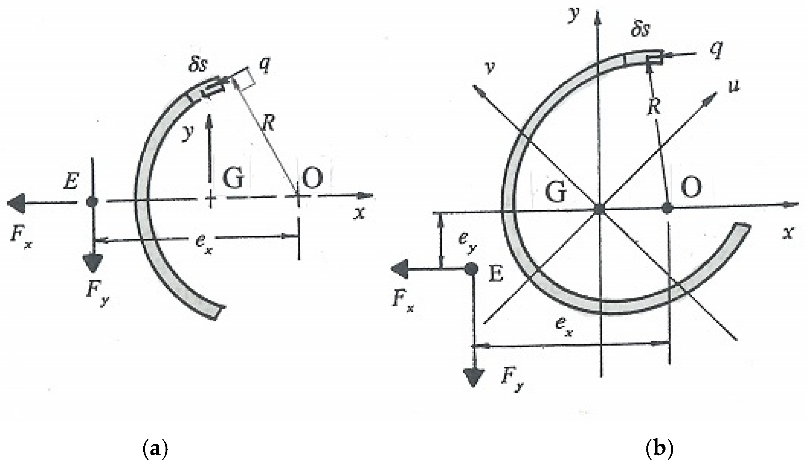
• Note (3): The net shear stress (Equation (7)) has a linear distribution through the thickness. The flexural shear flow, q_F, provides the mean shear stress at mid thickness. With q_F, the shear flow due to axial torsion q_T is superimposed to give a linear thickness variation in q_net between the free edges.

3. Torsional Shear Flow Calculations

This analysis begins with the application of Equation (5b) to an x axially symmetric channel section of uniform thickness. At a given position z along the beam’s length, the torsional shear flow in the cross-section is controlled by the integral Q, with torque T applied to shear centre E (see Figure 2a). The swept area diagram (see Figure 2b) provides Q at points 1, 2, 3 and 4 within each straight length 1–2, 2–3, etc., of the channel section. To permit different channel geometries, each Q appears finally in a non-dimensional form involving the ratios between channel dimensions a, d, e and t as follows:

1–3: 0 ≤ s ≤ a; ꞷ = ds/2; Q1–3 = ∫s (ds/2 − ϖ)ds = ds2/4 − ϖs

Q1 = 0, Q3 = da2/4 − ϖa; | Q3/a3 = (1/4)(d/a) − ϖ/a2

3–4: a ≤ s ≤ a + d/2; ꞷ = es + (ad/2 − ea); Q3–4 = ∫s [es + (ad/2 − ea) − ϖ] ds

Q4/a3 = (1/2)(e/a)[1 + (1/2)(d/a)]2 + (ko/a2 − ϖ/a2)[1 + (1/2)(d/a)] + k1/a3

4–5: a + d/2 ≤ s ≤ a + d; y = −se + (ad/2 + ed + ea); Q4–5 = ∫s [−se + (ad/2 + ed + ea) − ϖ]ds

= ∫s (k3 −se − ϖ) ds

Q5/a3 = −(1/2)(e/a)(1 + d/a)2 − (ϖ/a2 − k3/a2)(1 + d/a) + k4/a3

5–7: a + d ≤ s ≤ 2a + d; ꞷ = −ds/2 + d(a + d/2); Q5–7 = ∫s [−ds/2 + d(a + d/2) − ϖ]ds

= ∫s (k5 −sd/2 − ϖ) ds

Q7/a3 = −(1/4)(d/a)(2 + d/a)2 − (2 + d/a)(ϖ/a2 − k5/a2) + k6/a3

where

ko/a2 = (1/2)(d/a) − (e/a)

k1/a3 = −(1/4)(d/a) + (1/2)(e/a)

k3/a2 = (e/a)(d/a) + e/a +(1/2)(d/a)

k4/a3 = (e/a)[1 + (1/2)(d/a)]2 + [1 + (1/2)(d/a)](ko/a2 − k3/a2) + k1/a3

k5/a2 = (d/a)[1 + (1/2)(d/a)]

k6/a3 = (1 + d/a)2[(1/4)(d/a) − (e/a)] + (1 + d/a)(k3/a2 − k5/a2) + k4/a3

∃/a2 = (1/4)(d/a)[2(1 + d/a) +(e/a)(d/a)]/(2 + d/a)

e/a = 3(a/d)/[1 + 6(a/d)]

The Q coefficients listed in

Table 1. Torsional Q distributions in three channel sections.

Section A: a = ½″, d = 1″, t = 1/16″, d/a = 2, ex/a = 3/8, ϖ/a2 = 27/32 ko/a2 = 1 − 3/8 = 5/8 k1/a3 = −(1/4) × 2 + (1/2)(3/8) = −5/16 k3/a2 = 3/4 + 3/8 + 1 = 17/8 k4/a3 = (3/8) × 4 + 2(5/8 − 17/8) − 5/16 = −29/16 k5/a2 = 2(1 + 1) = 4 k6/a3 = (3)2(1/2 − 3/16) + 3(17/8 − 4) − 29/16 = −74/16 Q1 = 0 Q3/a3 = (1/4) × 2 − 27/32 = −11/32 Q4/a3 = (3/16)(1 + 1)2 +(5/8 − 27/32) × 2 − 5/16 = 0 (check) Q5/a3 = −(3/16) × 32 − (27/32 − 17/8) × 3 − 29/16 = 11/32 Q7/a3 = −(1/2) × 16 − 4(27/32 − 4) − 74/16 = 0 (check)

Section B: a = 1″, d = 1¾″, t = ⅛″, d/a = 7/4, ex/a = 12/31, ϖ/a2 = 0.7207 ko/a2 = 7/8 − 12/31 = 0.488 k1/a3 = (1/4)(7/4 − 24/31) − 0.488 = −0.244 k3/a2 = (12/31 × 7/4) + 12/31 + (1/2)(7/4) = 1.9375 k4/a3 = (12/31)(1 + 7/8)2 + (1 + 7/8)(0.488 − 1.9375) − 0.244 = −1.6047 k5/a2 = (7/4)(1 + 7/8) = 3.2813 k6/a3 = (11/4)2(7/16 − 12/62) + (11/4)(1.9375 − 3.2813) − 1.6037 = −3.4498 Q1 = 0 Q3/a3 = (1/4)(7/4) − 0.7207 = −0.2832 Q4/a3 = (12/62)(1 + 7/8)2 + (0.488 −0.7207)(1 + 7/8) − 0.244 = 0 (check) Q5/a3 = −(12/62)(11/4)2 − (0.7207 − 1.9395)(11/4) −1.6047 = 0.2832 Q7/a3 = −(7/16)(2 + 7/4)2 − (2 + 7/4)(0.7207 −3.2813) − 3.4498 = 0 (check)

Section C: a = ⅝″, d = 1⅞″, t = 3/64″, d/a = 3, ex/a = 1/3, ϖ/a2 = 27/20 ko/a2 = 3/2 − 1/3 = 7/6 k1/a3 = (1/4)(3 −2/3) − 7/6 = −7/12 k3/a2 = 3/2 + 1 + 1/3 = 17/6 k4/a3 = (1/3)(1 + 3/2)2 + (1 + 3/2)(7/6 − 17/6) − 7/12 = −8/3 k5/a2 = 3(1 + 3/2) = 15/2 k6/a3 = 16(3/4 −1/6) + 4(17/6 − 15/2) − 8/3 = −12 Q1 = 0 Q3/a3 = 3/4 −27/20 = −3/5 Q4/a3 = 1/6(1 + 3/2)2 + (7/6 −27/20)(1 + 3/2) − 7/12 = 0 (check) Q5/a3 = −(1/6)(16) − (27/20 −17/6)4 − 8/3 = 3/5 Q7/a3 = −3/4(25) − 5(27/20 −15/2) − 12 = 0 (check)

above are proportional to the shear flow within each channel section. Shear flow q (N/mm) at positions 1, 2, … 7 in the channel wall are found from multiplying Q (mm³) by Et (d³θ/dz³) (N/mm⁴). Then, the shear stress at these positions follows from τ = q/t = E(d³θ/dz³). Equation (6c) shows that the third derivative depends upon z and q = cQ within the proportionality referred to.

Table 2. Torsional shear flow dependence upon length within three channel sections A, B and C with torsion applied at E.

Successive Normalised Length Ratios
z/L	0	1/4	1/2	3/4	1
1 − z/L	1	3/4	1/2	1.4	0
(A) μL(1 − z/L)	1.9685	1.4764	0.9843	0.4921	0
coshμL(1 − z/L)	3.65	2.303	1.5248	1.1236	1
coshμL(1 − z/L)	1	0.631	0.4178	0.3078	0.274
coshμL
(G/T) d3θ/dz3 × 106	−0.6357	−0.4011	−0.2656	−0.1957	−0.1742
(B) μL(1 − z/L)	4.55	3.4125	2.275	1.1375	0
coshμL(1 − z/L)	47.32	15.187	4.9154	1.7198	1
coshμL(1 − z/L)	1	0.3209	0.1039	0.03634	0.02113
coshμL
(G/T) d3θ/dz3 × 109	−20.4	−6.533	−2.1155	0.7399	−0.4302
(C) μL(1 − z/L)	0.936	0.702	0.468	0.234	0
coshμL(1 − z/L)	1.471	1.2567	1.1115	1.0275	1
coshμL(1 − z/L)	1	0.8543	0.7556	0.6985	0.6798
coshμL
(G/T) d3θ/dz3 × 106	−0.167	0.1426	−0.1261	−0.1166	−0.1135

shows how d³θ/dz³ varies with z/L in each channel section for a unit torque, using constants J and µ. From Equation (6c),

d³θ/dz³ = −(T/GJ) [μ²coshμ(L − z)/cosh μL]

(8a)

(G/T) d³θ/dz³ = −(μ²/J)cosh[μL(1 − z/L)]/cosh μL

(8b)

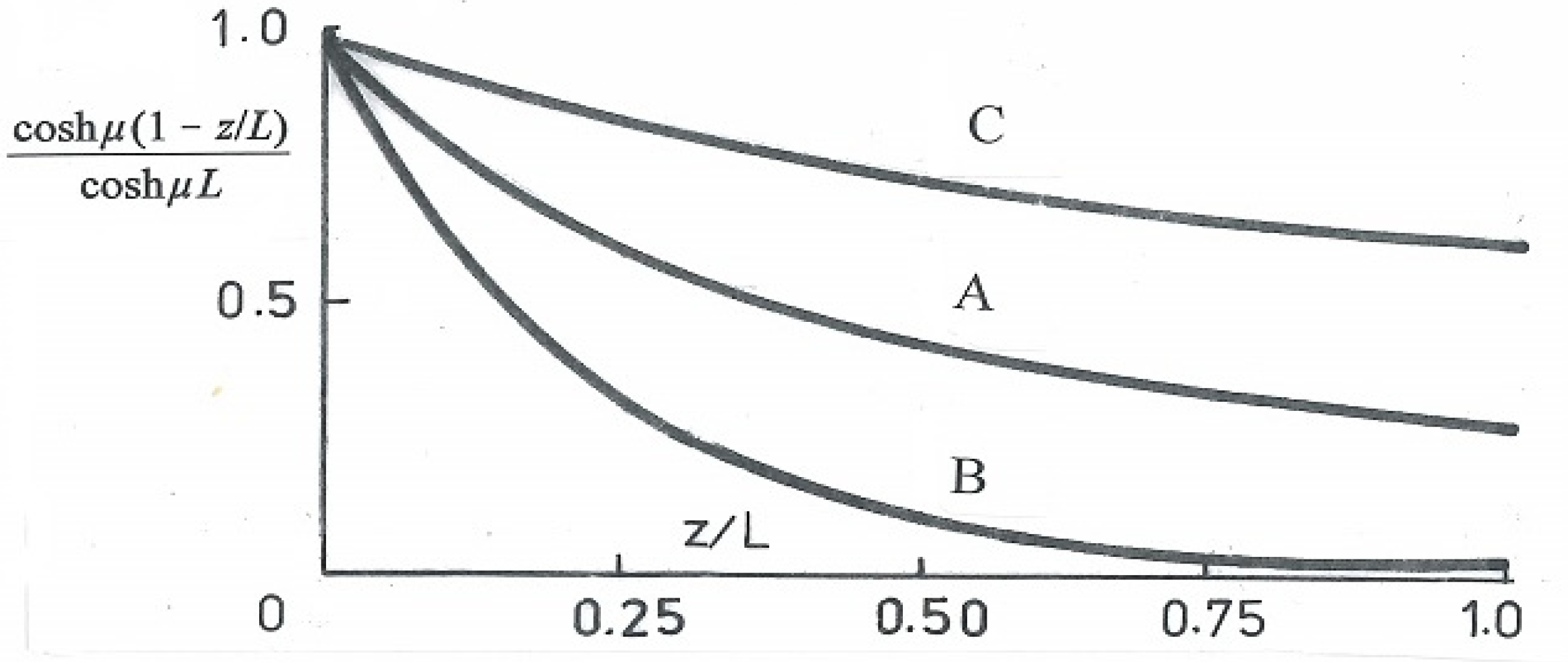
• A: J = 67.74 mm⁴, µ = √(GJ/EΓ₁) = 6.562 × 10⁻³ mm⁻¹, µL = 6.562 × 10⁻³ × 300 = 1.9685;
• B: J = 1016.8 mm⁴, µ = √(GJ/EΓ₁) = 4.55 × 10⁻³ mm⁻¹, µL = 4.55 × 10⁻³ × 10³ = 4.55;
• C: J = 44.656 mm⁴, µ = √(GJ/EΓ₁) = 2.73 × 10⁻³ mm⁻¹, µL = 2.73 × 10⁻³ × 340 = 0.936.

The hyperbolic dependence of a given section’s torsional shear flow upon length and cross-section geometry appears in the penultimate row for A, B and C in Table 2. There is sufficient variation in geometry between the three channels to reveal both the influence of the cross-section and the length (through L and μ) upon shear flow within Figure 3.

The greatest beam length of 1 m for section B shows the widest variation in shear flow, with this being near zero at the free end. Reducing this length to ≈ 1/3 for A and C shows how their channel section dimensions alter the fall in shear flow from the fixing by ≈ 27% and 68% at the free end, respectively.

The torsional shear flow at perimeter points i = 1, 2 … 7 for each cross-section at a given length position is found from multiplying the entry in the final row in Table 2 for each channel A, B and C by the appropriate Q_i values (see Equation (5b,c)). Thus, for channel section A at half length, the entry of −0.2656 applies to the section’s q distribution under a unit torque (T = 1 Nm) with E/G = 210/70 = 3, as follows:

qi = Et (d3θ/dz3)Qi = Et × (− 0.2656 × 10−6)T/G × Qi

= 3 × (1/16 × 25.4) × (− 0.2656 × 10−6) × (1 × 103) × Qi

= −(1.265 × 10−3) Qi

where, as calculated previously,

Q₁ = 0, Q₃ = −(11/32)a³, Q₄ = 0, Q₅ = (11/32)a³, Q₇ = 0

giving

q1 = q4 = q7 = 0 ∴ q3 = −q5 = −(1.265 × 10−3) × (−11/32)(1/2 × 25.4)3 = 0.891 N/mm

The torsional q_T distribution has convex curvature within the channel reflecting at the web centre (e.g., see Figure 6c). To this, there is to be added the flexural shear flow from F_x and F_y re-applied together at E (in the negative x and y directions). Recall that this summation of torsion and shear amounts to adopting a force system equivalent to that of applying these forces to the centroid directly. That is, when, as here, F_x and F_y are applied to G in Figure 4a, they are equivalent to re-applying said forces at E with an accompanying torque, T = F_y(e_x + X′), as shown in Figure 4b. Torsion is absent only when the transverse forces are applied directly to E. Thus, either equivalent force system in (b) and (c) provides an alternative calculation for q_net in (a).

Here, with section symmetry, bending moments arising from F_y, which act about axis x, pass through both G are E. This paper later questions in Section 9.8 whether bending moments arising from F_x and acting about axis y through G in Figure 4a are altered by the parallel transfer of the y-axis to E. With section asymmetry, such a ‘trans-moment’ would appear possible with the transfer of each non-coincident axis between G and E. Normally, the static equivalence that Figure 4a,b show does not account for any change to the bending moments that a shift in their forces might produce, i.e., Figure 4a,b do not include bending. The trans-moment is introduced here as a novel theoretical feature for which stress calculations for each type of section are to follow (see Section 9.8).

4. Flexural Shear Flow

Here, Figure 4a,b apply to each uniformly thick, singly symmetric, channel A, B and C, having x and y as its principal axes with aligned forces F_x and F_y applied at centroid G. Working along the mean centre line of an x-symmetric channel, web d × t and flanges a × t, centroid position X′ and the second moments of area for centroidal axes x and y in Figure 5a,b appear in their ND forms X′/a, I_x/d ⁴ and I_y/d ⁴:

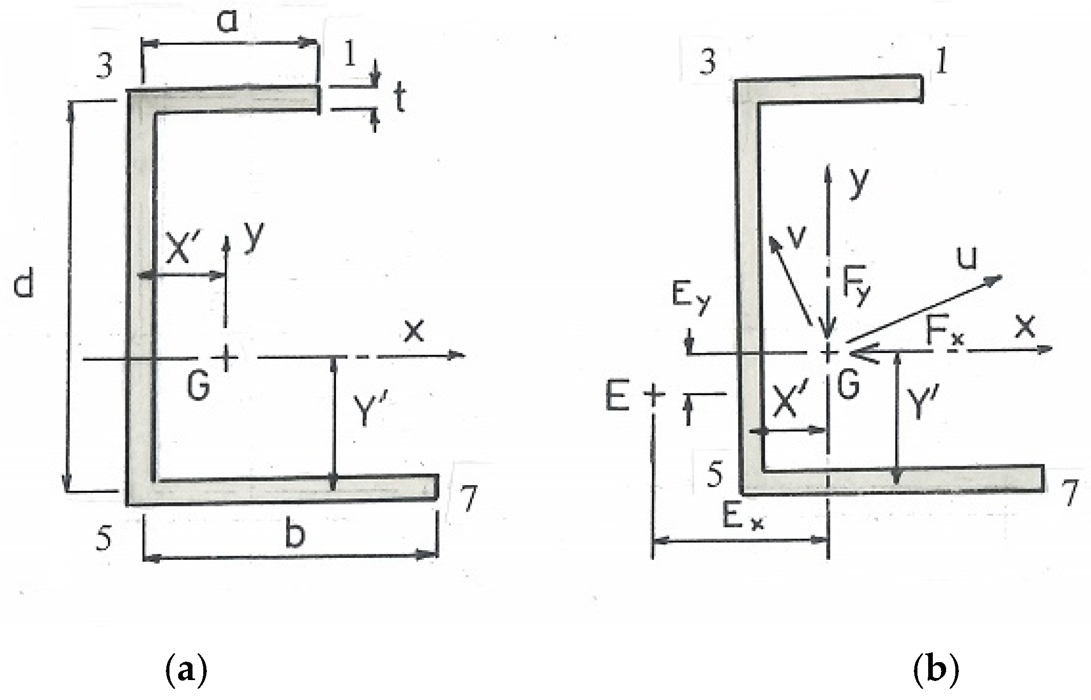
X′/a = (a/d)/[1 + 2(a/d)] Ix = 2[at(d/2)2 + at3/12] + td3/12 = atd2/2 + at3/6 + td3/12 Ix/d4 = (1/2)(a/t)(t/d) + (1/6)(a/d)(t/d)3 + (1/12)(t/d) Iy = dt3/12 + dtX′2 + 2[ta3/12 + at (a/2 − X′)2] Iy/d4 = (1/12)(t/d)3 + (t/d)(X′/d)2 + 2{(1/12)(t/d)(a/d)3 + (a/d)(t/d)[(1/2)(a/d) − (X′/d)]2}

Each ND form employs the dimension ratios a/d, t/d and X′/d for any x-symmetric channel geometry. The first moment of area integrals D_x and D_y in Equation (2a) follow separately as

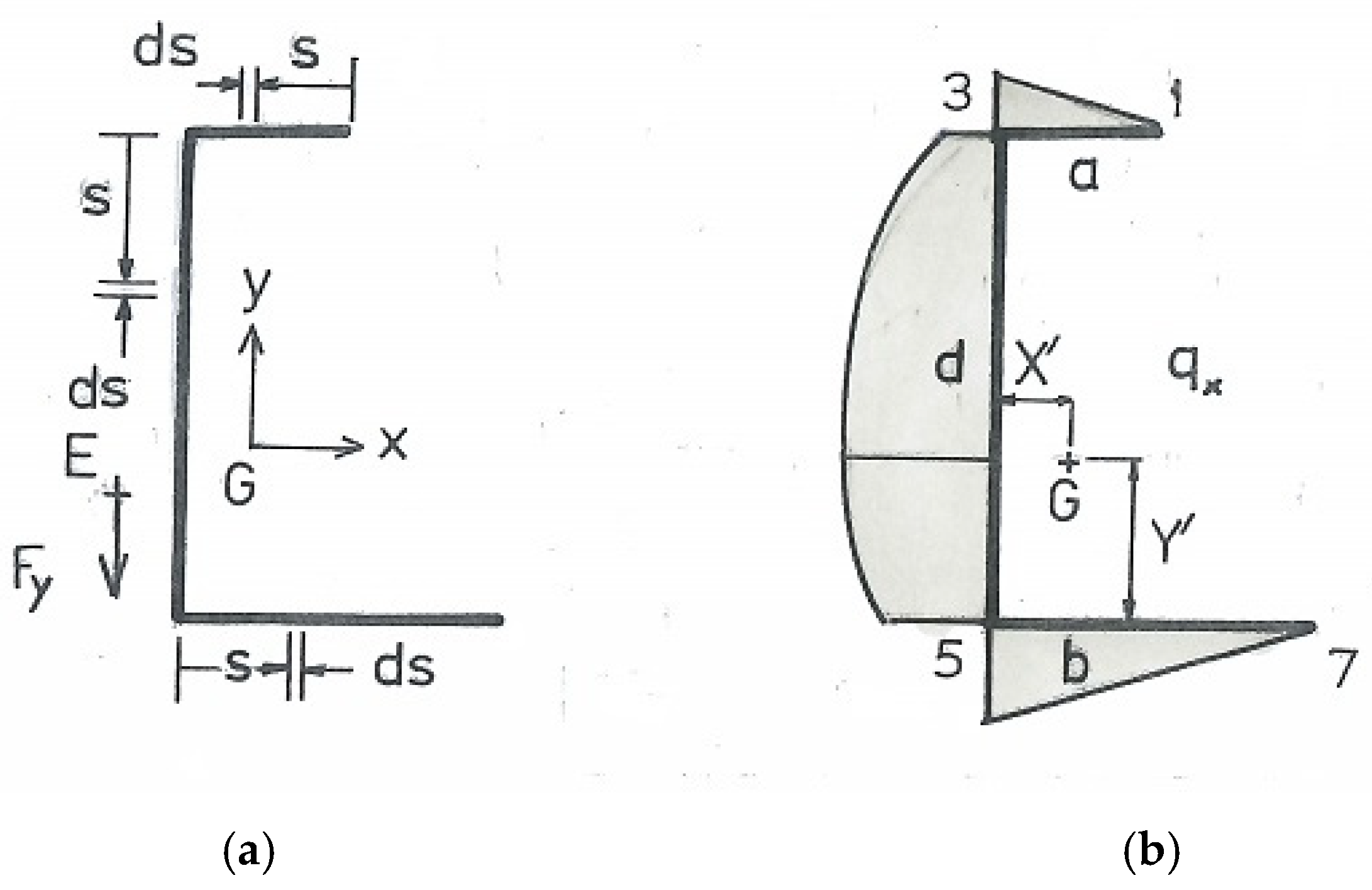
1–3: Dx = t ∫s y ds = tds/2 + Dx1 at 1, s = 0, Dx1 = 0 (free edge) at 2, (y–axis), s = a −X′, Dx2 = td (a −X′)/2 at 3. s = a, Dx3 = tda/2 3–5, Dx = t ∫s (d/2 − s) ds = t(ds/2 − s2/2) + Dx3 at 3, s = 0, Dx3 = tda/2 at 4, (x-axis) s = d/2, Dx4 = t(d2/4 −d2/8) + tda/2 = td2/8 + tda/2 ✓ (NA, web centre) at 5, s = d, Dx5 = Dx3 = tda/2 5–7 Dx = −t ∫s (d/2) ds + Dx5 = −tds/2 + Dx5 at 5, s = 0, Dx = Dx5 = tda/2 at 6, (y-axis), s = X′, Dx6 = −tdX′/2 + tda/2 = Dx2 at 7, s = a, Dx7 = −tda/2 + tda/2 = 0 ✓ (at the free edge)

Given that D_x is proportional to q_x, Figure 5a shows that the q_x distribution is linear between flange points 1, 2 and 3 and between 5, 6 and 7. Web points, 3, 4 and 5 connect q with a convex parabola, showing maximum shear flow upon the neutral axis (NA) at point 4 on the section’s centroidal axis.

To find the q_y distribution (Figure 5b), take s counter-clockwise direction with the origin initially at free end point 1 on the top flange, where D_y = 0, and thereafter at median points 2, 3 … 7:

1–3: Dy = t ∫s[a − (s + X′)] ds = (a −X′)s − s2/2 + Dy1 at 1, s = 0, Dy1 = 0 at 2 (y–axis, NA), s = a − X′, Dy2 = t [(a − X′)2 − (a − X′)2/2] = (t/2)(a − X′)2 at 3, s = a, Dy3 = t [(a − X′)a − a2/2] = at(a/2 − X′) 3–5: Dy = −t ∫s X′ ds + Dy3 = −t X′ s + Dy3 at 3, s = 0, Dy3 = at(a/2 − X′) at 4 (x-axis), s = d/2, Dy4 = a2t/2 − X′ t (a + d/2) at 5, s = d, Dy5 = −t X′ d + at (a/2 − X′) = a2t/2 − X′ t (a + d) 5−7: Dy = −t ∫s(s −X′) ds + Dy5 = ts (s/2 − X′) + Dy5 at 5: s = 0, Dy5 = a2t/2 − X′ t (a + d) at 6 (y–axis, NA): s = X′, Dy6 = X′ t (X′/2 −X′) + a2t/2 −X′ t (a + d) Dy6 = (a2t/2) −X′ t (X′/2 + d + a) at 7, s = a, Dy7 = ta (a/2 − X′) + a2t/2 −X′ t (a + d) = a2t −X′ t (2a + d)

Substituting for X′ leads to the D_y first moment expressions for each point 1–6:

Dy1 = 0 Dy2 = (at2/2)[(a + d)/(2a + d)]2 (y-axis, NA) Dy3 = (at2/2)d/(2a + d) Dy4 = a2t/2 − X′ t (a + d/2) = 0 (x-axis) Dy5 = (at2/2)[1 − 2(a + d)/(2a + d)] = Dy3 Dy6 = (a2t/2) −X′ t (X′/2 + d + a) = (a2t/2)[1 − a2/(2a + d)2 − 2(a + d)/(2a + d)] = Dy2 Dy7 = a2t − a2t(2a + d)/(2a + d) = 0 ✓

Figure 5b shows that top flange points 1, 2 and 3 lie on a convex parabola that has its zero origin at the free edge 1 and a maximum at point 2 on the NA (y-axis). Points 3, 4 and 5 connect with a straight line showing q_y = 0 at point 4 on the x-axis. Points 5, 6 and 7 connect with a convex parabola with a maximum at point 6 on the NA (y-axis) reducing to zero at flange end point 7, as expected. This distribution has inverted symmetry, indicating that the shear flow positive direction is reversed below point 4 compared to the direction taken for the perimeter dimension s (here counter-clockwise). That is, symmetry in q_y applies when the direction of s beyond the NA at point 4 is reversed. Alternatively, for the bottom half of the channel, s may start from point 7 taken clockwise as far as the NA. Note: the q_y distribution may be ‘added’ to q_x only when the direction for s is the same in Figure 5a,b as shown.

5. Net Flexural Shear Flow

The net flexural shear flow is the sum of the shear flows due to transverse forces F_x and F_y taken separately. The following sum follows from Equation (2a):

q_x + q_y = (F_x/I_y)D_y + (F_y/I_x)D_x

(9a)

When the forces and second moments of area are written as ratios, the two flexural shear flows may be added to include the product of these ratios:

(q_x + q_y)(I_y/F_x) = D_y + (F_y/F_x)(I_y/I_x)D_x

(9b)

The I_x and I_y values for the three channels, A, B and C, are given in

Table 3. Geometric properties of three x-symmetric channel sections.

Section A: a = 1/2″, d = 1″, t = 1/16″, L = 300 mm (11.81″) a/d = ½, a/t = 8, t/d = 1/16, X′/a = 1/4, X′/d = 1/8, ex/a = 3/8 Ix = 0.02055d4; Iy = 0.00328d4, Iy/Ix = 0.1571, ϖ/a2 = 27/32

Section B: a = 1″, d = 1¾″, t = ⅛″, L = 1 m (39.37″) a/d = 4/7, a/t = 8, t/d = 1/14, X′/a = 4/15, X′/d = 16/105, ex/a = 12/31 Ix = 0.026375d4; Iy = 0.0053615d4, Iy/Ix = 0.20315, ϖ/a2 = 0.7207

Section C: a = 5/8″, d = 1⅞″, t = 3/64″, L = 340 mm (13.39″) a/d = 1/3, a/t = 40/3, t/d = 1/40, X′/a = 1/5, X′/d = 1/15, ex/a = 1/3 Ix = 0.006251d4; Iy = 0.0004334d4, Iy/Ix = 0.06934, ϖ/a2 = 27/20

with their respective geometrical ratios.

Here, in general, the following expressions for each section’s geometric properties apply:

X′/a = (a/d)∕[1 + 2(a/d)] ex/a = 3(a/d)∕[1 + 6(a/d)] ϖ/a2 = (1/4)(d/a)[2(1 + d/a) + (e/a)(d/a)]∕(2 + d/a) Ix = 2[at(d/2)2 + at3/12] + td3/12 = atd2/2 + at3/6 + td3/12 Ix/d4 = (1/2)(a/d)(t/d) + (1/6)(a/d)(t/d)3 + (1/12)(t/d) Iy = dt3/12 + dtX′2 + 2[ta3/12 + at(a/2 − X′)2] Iy/d4 = (1/12)(t/d)3 + (t/d)(X′/d)2 + 2{(1/12)(t/d)(a/d)3 + (a/d)(t/d)[(1/2)(a/d) − (X′/d)]2}

The individual shear flows, q_x and q_y, for each channel section A, B and C are as shown in Figure 5a,b when, respectively, F_x and F_y are taken separately to act at the channel section’s centroid G. As an example of applying Equation (9b), if the force ratio F_y/F_x is unity, the net flexural shear flow at the N.A. (x–axis) for section A follows from a weighted addition of D_x and D_y between Figure 5a,b:

(Iy/Fx)qnet = Dy + (Fy/Fx)(Iy/Ix)Dx = [a2t/2 − X′ t (a + d/2)] + (1 × 0.1571)(td2/8 + tda/2) = [(1/2)(a/d)2(t/d) − (X′/d)(t/d)(a/d + 1/2)]d3 + 0.1571[(1/8)(t/d) + (1/2)(t/d)(a/d)]d3 = [(1/2)(1/2)2(1/16) −(1/8)(1/16)(1/2 + 1/2)]d3 + 0.1571[(1/8)(1/16) + (1/2)(1/16)(1/2)]d3 = 0 + (3.682 × 10−3) d3

in which D_y = 0. Hence, D_x only is responsible for the net flexural shear flow at NA:

q_net = (F_x/I_y) (3.682 × 10⁻³)d³ = F_x(3.682 × 10⁻³)d³∕(3.28 × 10⁻³)d⁴ = 1.1226F_x/d

which, for shear forces of F_y = F_x = 100 N (say) applied to G, with d = 25.4 mm, gives:

qnet = 1.1226 × 100/25.4 = 4.42 N/mm ∴ τ = qnet/t = 16 × 4.42 = 70.7 MPa

6. Net Shear Flow

The net shear flow is the sum of the flexural and torsional shear flows. Applying this sum to the example calculation considered above, force F_y corresponds to a torque applied at E:

T = F_y (e_x + X′) = 100 (3/8 + 1/4)12.7 = 793.75 N mm

in which F_x does not contribute to T (e_y = 0). Figure 6c shows that there is no q_T shear flow at the NA due to torsion. Hence, the net shear stress of 70.7 MPa upon the NA arises from q_x = 4.42 N/mm only. By contrast, Figure 6c shows that the maximum shear flow due to torsion occurs at the fixing for this section at corner points 3 and 5. To show this, the magnitudes follow by proportion from Table 1 as

q_T = (793.75/1000) × 0.6357/0.2656 × (±0.891) = ±1.692 N/mm

The flexural and torsional shear flow sum (N/mm) at all points 1, 2 … 7 around this fixed-end section’s mean perimeter is given as ∑q in

Table 4. Net shear flow ∑q, (N/mm) and shear stress τ, MPa for channel section A with transverse force F_x = F_x applied to centroid G.

Point	1	2	3	4	5	6	7
Dy/d3	0	1/227.55	1/256	0	−1/256	−1/227.55	0
Dx/d3	0	3/256	1/64	3/128	1/64	3/256	0✓
× Iy/Ix	0	1/543.18	1/407.38	1/271.59	1/407.38	1/543.18	0
∑D/d3	0	1/160.37	1/157.21	1/271.59	−1/688.92	−1/391.6	0
qx + qy	0	7.485	7.636	4.420	−1.742	−3.065	0
qT	0	1.731	1.692	0	−1.692	−1.731	0✓
∑q	0	9.216	9.328	4.420	−3.434	−4.796	0
τ =∑q/t	0	5.805	5.876	2.784	−2.163	−3.021	0

, calculated as

∑q = q_x + q_y + q_T

Figure 6a–c shows separately the three shear flows that arise from applying the two forces F_x and F_y at G. These are the two flexural shear flows, q_x and q_y, (Figure 6a,b), and one torsional shear flow, q_T (Figure 6c), due to force F_y being offset from the shear centre. Each diagram plots the shear flow magnitude, given in Table 4, vertically between 1 and 3, 3 and 5 and 5 and 7 on the sections median line (bold). To find the net shear flow, a weighted sum must apply to D_x and D_y in Figure 6a,b (by using Equation (9b)) before adding to q_T. The separate ordinates q_x, q_y and q_T (N/mm) are presented diagrammatically in Figure 6a–c for which their sum is shown in Figure 6d. The final row in Table 4 provides the net shear stress τ = ∑q/t numerically. This reveals the net shear stress distribution, τ, (MPa) for fixed-end channel section A when ∑q is divided by t = 1.5875 mm (1/16″).

Table 5. Net shear flow ∑q, (N/mm) and shear stress τ, MPa, for channel section B with transverse forces F_x = F_x = 100 N applied to centroid G. (‘check’ means the result is expected)

Point	1	2	3	4	5	6	7
Dy/d3	0	6.27 × 10−3	5.42 × 10−3	0	−5.42 × 10−3	−6.27 × 10−3	0
Dx/d3	0	14.97 × 10−3	20.41 × 10−3	29.34 × 10−3	20.41 × 10−3	14.97 × 10−3	0 (check)
×Iy/Ix	0	3.337 × 10−3	4.146 × 10−3	5.96 × 10−3	4.146 × 10−3	3.337 × 10−3	0
∑D/d3	0	9.607 × 10−3	9.566 × 10−3	5.96 × 10−3	−1.274 × 10−3	2.933 × 10−3	0
qx + qy	0	4.0312	4.0139	2.5009	−0.5345	−1.2307	0
qT	0	1.550	1.497	0	−1.497	−1.550	0 (check)
∑q	0	5.5812	5.5109	2.5009	−2.0315	−2.7807	0
τ = ∑q/t	0	1.758	1.736	0.7877	−0.64	−0.8758	0

and

Table 6. Net shear flow ∑q, (N/mm) for channel section C with transverse forces F_x = F_x = 100 N applied to centroid G.

Point	1	2	3	4	5	6	7
Dy/d3	0	8.88 × 10−4	8.333 × 10−4	0	−8.333 × 10−3	−8.88 × 10−4	0
Dx/d3	0	33.33 × 10−4	41.7 × 10−4	72.92 × 10−4	41.7 × 10−4	33.33 × 10−4	0 (check)
×Iy/Ix	0	2.311 × 10−4	2.892 × 10−4	5.056 × 10−4	2.892 × 10−4	2.311 × 10−4	0
∑D/d3	0	11.191 × 10−4	11.225 × 10−4	5.056 × 10−4	−5.441 × 10−4	−6.569 × 10−4	0
qx + qy	0	5.4218	5.4383	2.4495	−2.6361	−3.1826	0
qT	0	1.23	1.23	0	−1.23	−1.23	0 (check)
∑q	0	6.652	6.668	2.450	−3.866	−4.413	0
τ = ∑q/t	0	5.587	5.60	2.458	−3.247	−2.707	0

further reveal the net shear stress distribution, τ, (MPa) for fixed-end beams with sections B and C, calculated in a similar manner. These require ∑q to be divided by t = 3.175 mm (1/8″) and 1.1906 mm (3/64″), respectively.

Table 4, Table 5 and Table 6 show how the ∑q distribution depends upon each channel section’s geometry and beam length under a similar transverse unit force ratio. These distributions apply to the end fixing where ∑q values are at their greatest. The conversion to net shear stress τ = ∑q/t in the final row of each table shows that these are of low magnitude given in MPa (=N/mm²). Nonetheless, their contribution to the safety of the structure must be considered along with the net axial stress (to follow) in a suitable criterion of buckling/yielding. For example, the yield criteria of Tresca and von Mises apply to a ductile metal in which the yield stresses for the aluminium alloy are 250 MPa in tension and 150 MPa in shear (see Section 8).

7. Net Axial Stress

The net axial stress at a length position, z, is the sum of the bending stresses due to moments M_x = F_y(L − z) and M_y = F_x(L − z), taken from Equation (1a−c), added to the axial stress at that position induced by constraining all warping displacement at the fixed end (z = 0). Bending stresses under M_x and M_y in Figure 7a are aligned with the length direction z. Figure 7b shows how σ_z is distributed linearly over the section’s depth d, under M_x. Under M_y a linear distribution in σ_z applies across the flange width, b. Both distributions are zero, i.e., ‘neutral’ to stress at their intersections with centroidal co-ordinates x and y.

The signs of bending stresses σ_z in Equation (7) complies with a hogging moment producing tension (y positive) and sagging moment compression (y negative). Signs of σ_z, denoting tension (+) and compression (−), are referred to the section’s quadrants whose centroidal axes x and y carry hogging moments M_x and M_y as shown. Conveniently, here, forces F_x and F_y applied to G in negative x and y directions each produce hogging moments in the first quadrant, i.e., 1(+, +). In the remaining quadrants, their respective signs are: 2(+, −), 3(−, −) and 4(−, +).

7.1. Net Bending Stress

When forces F_x and F_y are aligned with the section’s principal directions (x and y), the combined axial stress arising from M_x and M_y within each quadrant’s points in the channel section is as follows:

σ_z = ± M_x y/I_x ± M_y x/I_y

(10)

Quadrant 1: points 1 and 2: σ_z = + F_y(L − z)y/I_x + F_x(L − z)x/I_y

(11a)

Quadrant 2: points 2, 3 and 4: σ_z = + F_y(L − z)y/I_x − F_x(L − z)x/I_y

(11b)

Quadrant 3: points 4, 5 and 6: σ_z = −F_y(L − z)y/I_x − F_x(L − z)x/I_y

(11c)

Quadrant 4: points 6 and 7: σ_z = −F_y(L − z)y/I_x + F_x(L − z)x/I_y

(11d)

in which the respective signs are simply those of the co-ordinates (x, y) across the four quadrants in this convention. It can be seen from Equation (11a–d) that the net bending stress distribution is 3D, for which Figure 7a,b are its 2D projection in the z–y plane. To show the 3D distribution in an oblique view, median perimeter points 1, 2, 3 … 7 lie along the channel’s mid-thickness in which the following co-ordinates (with signs) in

Table 7. Perimeter point co-ordinates with quadrant signs for bending.

Point	1	2	3	4	5	6	7
x	a − X′	0	−X′	−X′	−X′	0	a − X′
y	d /2	d /2	d /2	0	−d/2	−d/2	−d/2

apply.

Substituting from Table 7, Equation (11a–d) are re-written, for F_x = F_y = F, in non-dimensional form to provide for specific channel constants and length ratios as follows:

(d⁴/a)(σ_z1/FL) = (1/2k_x)(d/a) + (1 − X′/a)/k_y

(12a)

(d⁴/a)(σ_z2/FL) = (1/2k_x)(d/a)

(12b)

(d⁴/a)(σ_z3/FL) = (1/2k_x)(d/a) − (X′/a)/k_y

(12c)

(d⁴/a)(σ_z4/FL) = −(X′/a)/k_y

(12d)

(d⁴/a)(σ_z5/FL) = −(1/2k_x)(d/a) − (X′/a)/k_y

(12e)

(d⁴/a)(σ_z6/FL) = −(1/2k_x)(d/a)

(12f)

(d⁴/a)(σ_z7/FL) = −(1/2k_x)(d/a) + (1 − X′/a)/k_y

(12g)

Note: Constants k_x and k_y appear in the second moment of area expressions I_x = k_xd⁴ and I_y = k_yd⁴ (with units in mm⁴) for each channel as follows.

Channel A: d/a = 2, X′/a = 1/4, k_x = 0.02085, k_y = 0.003276, L = 300 mm and d = 25.4 mm. Substituting into Equation (12a–g) leads to the net bending stress (in MPa) at each mid-thickness perimeter position.

(d4/a)(σz1/FL) = 1/(2 × 0.02085)(2) + (1 − 1/4)/0.003276 = 276.9, |σz1 = 2534.6 × 10−3F (d4/a)(σz2/FL) = 1/0.02085 = 47.96, |σz2 = 439 × 10−3F (d4/a)(σz3/FL) = 1/0.02085 − 0.25/0.003276 = −28.35, |σz3 = −259.5 × 10−3F (d4/a)(σz4/FL) = −0.25/0.003276 = −76.31, |σz4 = −698.5 × 10−3F (d4/a)(σz5/FL) = −1/0.02085 − 0.25/0.003276 = −124.27, σz5 = −1137.5 × 10−3F (d4/a)(σz6/FL) = −1/0.02085 = −47.96, |σz6 = −439 × 10−3F (d4/a)(σz7/FL) = −1/0.02085 + 0.75/0.003276 = 180.97, |σz7 = 1656.5 × 10−3F

where it can be seen that with F = 100 N, these stress levels are elastic, e.g., σ_z2 = 43.9 MP, (but not so if F = 1000 N). Figure 8 displays the elastic axial stress levels calculated above as a distribution connecting linear segments between perimeter points 1 and 2, 3 and 5 and 5 and 7. The arrows shown indicate the stress direction and the sense shows where the web and flanges receive their greatest compression and tension with equal forces F applied at G.

Channel B:

d/a = 7/4, X′/a = 4/15, k_x = 0.026395, k_y = 0.0053615, L = 1 m and d = 44.45 mm, a = 25.4 mm. When Equation (12a–g) are applied to channel section B, the bending stresses at each perimeter point are

(d4/a)(σz1/FL) = (1/0.026395 × 7/8) + (1/0.0053615 × 11/15) = 169.9, |σz1 = 1105.65 × 10−3F (d4/a)(σz2/FL) = (1/0.026395 × 7/8) = 33.1502, |σz2 = 215.69 × 10−3F (d4/a)(σz3/FL) = (1/0.026395 × 7/8) − (1/0.0053615 × 4/15) = 16.587, |σz3 = −107.92 × 10−3F (d4/a)(σz4/FL) = −(1/0.0053615 × 4/15) = −49.74, |σz4 = −323.6 × 10−3F (d4/a)(σz5/FL) = −(1/0.026395 × 7/8) − (1/0.0053615 × 4/15) = −82.888 |σz5 = −539.31 × 10−3F (d4/a)(σz6/FL) = −(1/0.026395 × 7/8) = −33.105, |σz6 = −215.69 × 10−3F (d4/a)(σz7/FL) = −(1/0.026395 × 7/8) + (1/0.0053615 × 11/15) = 103.63, |σz7 = 674.27 × 10−3F

where again it can be seen from a similar distribution to Figure 8 that with F = 100 N, these stress levels are elastic. The increase in this section’s thickness dimension compensates for the greater length in maintaining acceptable stress levels under these loads (F_x = F_y = 100 N).

Channel C:

d/a = 3, X′/a = 1/5, k_x = 0.006251, k_y = 0.0004334, L = 340 mm and d = 47.625 mm, a = 15.875 mm. When Equation (12a–g) are applied to channel section C, the bending stresses at each perimeter point become

(d4/a)(σz1/FL) = (1/0.006251 × 3/2) + (1/0.0004334 × 4/5) = 2085.83, |σz1 = 2188.4 × 10−3F (d4/a)(σz2/FL) = (1/0.006251 × 3/2) = 239.96, |σz2 = 251.76 × 10−3F (d4/a)(σz3/FL) = (1/0.006251 × 3/2) − (1/0.0004343 × 1/5) = −221.51, |σz3 = −232.4 × 10−3F (d4/a)(σz4/FL) = −(1/0.0004343 × 1/5) = −461.47, |σz4 = −484.16 × 10−3F (d4/a)(σz5/FL) = −(1/0.006251 × 3/2) − (1/0.0004343 × 1/5) = −701.43, |σz5 = −735.92 × 10−3F (d4/a)(σz6/FL) = −(1/0.006251 × 3/2) = −239.96, |σz6 = −251.76 × 10−3F (d4/a)(σz7/FL) = −(1/0.006251 × 3/2) + (1/0.0004334 × 4/5) = 1605.91, |σz7 = 1684.9 × 10−3F

Again, with F = 100 N, the stress levels in Figure 8 are linear elastic. However, it should be noted here that these are not net axial stress values. The latter follow from the addition of axial stress arising from the fixing constraint to be considered next. Only then can the safe loading be assessed from the net shear and net axial stress combination.

7.2. Constrained Axial Stress Distribution

The axial stress distribution induced within the length due to constraining the torsional warping displacements fully at the fixed end has been described in [1]. There, it was shown that the fixed end, where z = 0, provides the maximum contribution to the axial stress for the full constraint

σ_z = −[(ꞷ − ϖ) T∕(µΓ₁)] (1 − e^−2μL)∕(1 + e^−2μL)

(13a)

where each channel section’s properties have been given previously (see Section 5 and Table 3 above). The specific properties required when applying Equation (13a) to channel cross-section A (with torque applied to E) appear as follows:

Channel A:

d/a = 2, ex/a = 3/8, L = 300 mm, a = 12.7 mm, t = 1.5875 mm, Γ1/a5t = 0.66275, ϖ/a2 = 0.8438, X′/a = 1/4, μ = 0.8189t/a2, μL = 0.8189(t/a)(L/a) = 2.418, (1 − e−2μL)/(1 + e−2μL) = 0.9842

Substituting into Equation (13a) leads to a parametric form for σ_z:

σ_z = −[(ꞷ − ϖ)T∕(0.8189t/a² × 0.66275a⁵t)] × 0.9842

(at²/T)σ_z = 1.8134 (0.8438 − ꞷ/a²)

(13b)

Taking the ordinates ꞷ/a² from in the swept area plot in Figure 2a,b, Equation (13b) is applied to points 1, 3 and 4 (NA) as follows:

at 1 ꞷ1 = 0, ∴ (at2/T)σz1 = 1.8135(0.8438 − 0) = 1.5303 at 3, ꞷ3 = ad/2, ∴ (at2/T)σz3 = 1.8135[0.8438 − (1/2)(d/a)] = −0.2834 at 4, ꞷ4 = (a + e)d/2, ∴ (at2/T)σz4 = 1.8135[0.8438 − (1/2)(d/a)(1 + e/a)] = −0.9633

With symmetry evident from Figure 2a, it follows that σ_z1 = σ_z7 and σ_z3 = σ_z5. Torque T upon axis E, corresponding to transverse shear forces F_x = F_y = 100 N at G, follows from

T/a = F_y(e_x/a + X′/a) = 100(3/8 + 1/4) = 62.5 N

Hence, the stresses at these positions within the channel fixing are as follows:

σz1 = 1.5303 (T/at2) = 1.5303 × 62.5/1.58752 = 37.95 MPa σz3 = 0.2834 (T/at2) = −0.2834 × 62.5/1.58752 = −7.04 MPa σz4 = −0.9633 (T/at2) = −0.9633 × 62.5/1.58752 = −23.89 MPa

The swept area diagram shows that the stresses at points 1, 3 and 4 are connected with linear segments and extended symmetrically to the section’s bottom half. Figure 9 shows the full 3D constrained axial stress distribution at the fixing. Note: Figure 8 and Figure 9 (revised) contribute to the net axial stress within different distributions.

A similar stress distribution to Figure 9 will apply to other positions within the length 0 < z < L but with reduced magnitude [1]. Maximum tension appears at the flange ends and maximum compression at the web centre. The stress levels are all relatively low compared to those from bending (see Figure 8) but are equally important to the safe design of this structure (see Section 8). Further calculations follow below for the constrained axial stress within the fixed ends of channels B and C:

Channel B:

d/a = 7/4, ex/a = 12/31, L = 1000 mm, a = 25.4 mm, t = 3.175 mm, Γ1/a5t = 0.448, ϖ/a2 = 0.7206, X′/a = 4/15, μ = 0.924t/a2, μL = 0.924(t/a)(L/a) = 4.5474, (1 − e−2μL)/(1 + e−2μL) = 0.99978.

Substituting into Equation (13a) leads to a non-dimensional form of σ_z:

(at²/t)σ_z = 2.2172(0.7206 − ꞷ/a²)

(13c)

Taking ꞷ/a² ordinates from Figure 5a, Equation (13c) applies to points 1, 3 and 4 (NA) as follows:

at 1, ꞷ1 = 0, ∴ (at2/T)σz1 = 2.2172(0.7206 − 0) = 1.5977 at 3, ꞷ3 = ad/2, ∴ (at2/T)σz3 = 2.2172[0.7206 − (1/2)(d/a)] = −0.3423 at 4, ꞷ4 = (a + e)d/2, ∴ (at2/T)σz4 = 2.2172[0.7206 − (1/2)(d/a)(1 + e/a)] = −1.0933

With symmetry evident in the swept area plot, it follows that σ_z1 = σ_z7 and σ_z3 = σ_z5. Torque T corresponding to transverse shear forces F_x = F_y = 100 N applied to E follows as

T /a = F_y(e_x/a + X′/a) = 100 (12/31 + 4/15) = 65.38 N

Hence, the constrained stresses at these positions within the channel fixing are as follows:

σz1 = 1.5977 (T/at2) = 1.5977 × 65.38/3.1752 = 10.36 MPa σz3 = 0.2834 (T/at2) = −0.3423 × 65.38/3.1752 = −2.22 MPa σz4 = −1.0933 (T/at2) = −1.0933 × 65.38/3.1752 = −7.09 MPa

These three stress calculations are sufficient to establish the spread in stress that arises over the section at the fixing where there is full constraint (see Figure 9).

Channel C:

d/a = 3, ex/a = 1/3, L = 340 mm, a = 15.875 mm, t = 1.19063 mm, Γ1/a5t = 1.6375, ϖ/a2 = 1.35, X′/a = 1/5, μ = 0.5825t/a2, μL = 0.5825(t/a)(L/a) = 0.9356, (1 − e−2μL)/(1 + e−2μL) = 0.7332.

Substituting into Equation (13a) leads to a non-dimensional form of σ_z:

(at²/t)σ_z = 0.7687(1.35 − ꞷ/a²)

(13d)

Taking ꞷ/a² ordinates from Figure 2b, Equation (13d) applies to perimeter points 1, 3 and 4 (NA) as

at 1 ꞷ1 = 0, ∴ (at2/T)σz1 = 0.7687 (1.35 − 0) = 1.0377 at 3, ꞷ3 = ad/2, ∴ (at2/T)σz3 = 0.7687 [1.35 − (1/2)(d/a)] = −0.1153 at 4, ꞷ4 = (a + e)d/2, ∴ (at2/T)σz4 = 0.7687 [1.35 − (1/2)(d/a)(1 + e/a)] = −0.4996

With symmetry evident in the swept area plot, it follows that σ_z1 = σ_z7 and σ_z3 = σ_z5. Here, torque T corresponding to transverse shear forces F_x = F_y = 100 N at E follows from

T /a = F_y (e_x/a + X′/a) = 100 (1/3 + 1/5) = 53.33 N

Hence, the stresses at these positions within the channel C fixing are as follows:

σz1 = 1.5977 (T/at2) = 1.0377 × 53.33/1.190632 = 39.04 MPa σz3 = 0.2834 (T/at2) = −0.1153 × 53.33/1.190632 = −4.34 MPa σz4 = −1.0933 (T/at2) = −0.49966 × 53.33/1.190632 = −18.80 MPa

These three stresses appear in their respective positions 1, 3 and 4 in the distribution shown in Figure 9.

Table 8. Fixed-end axial stress (MPa) due to constraint in three different channel section cantilevers.

Point	1	2	3	4	5	6	7
Channel A	37.95	4.12	−7.04	−23.89	−7.04	4.12	37.95
Channel B	10.36	1.14	−2.22	−7.09	−2.22	1.14	10.36
Channel C	39.04	4.34	−4.34	−18.80	−4.34	4.34	39.04

reveals the influence of channel section geometry and beam length within which are the three essential calculations given above along with others required to provide the constrained axial stress distribution for each fixed-end section.

Note: Points 1 and 7 and points 3 and 5 are ‘mirrored’ within Table 8. Stresses for points 2 and 6, upon the y-axis, are found from linear interpolation. It appears from Table 8 that the maximum axial stresses that arise from constraining warping displacement within the fixing are all well within the elastic range. However, the possibility of compressive elastic buckling in the web (for points 3, 4 and 5) should not be overlooked. For this, the net axial stress distribution is required as follows.

7.3. Net Axial Stress Distribution

The net axial stress, given as a three-part sum in Equation (3a), may be interpreted most simply as the sum of three separate distributions within which the sign changes across the four quadrants are accounted for. Referred to the fixed end (z = 0), this stress summation becomes

σ_z = −[(ꞷ − ϖ)T∕µΓ₁](1 − e^−2μL)∕(1 + e^−2μL) + M_xy/I_x + M_yx/I_y

(14)

where the counter-clockwise direction taken for s within the first (constraint) term must start and finish at the flange ends. As with each analysis, when equal free end loads F_x = F_y = F = 100 N are applied at G, the three distributions may be added. Taking the corresponding stress levels from Figure 9 for the first term and from Figure 8 for the sum of the second two terms (net bending stress),

Table 9. Net axial stress summations in sections (A), (B) and (C) from end constraint and bending.

Channel A	1	2	3	4	5	6	7
1st term, MPa	37.95	4.12	−7.04	−23.89	−7.04	4.12	37.95
2nd term, MPa	253.46	43.9	−25.93	−69.85	−113.75	−43.9	165.65
∑σz, MPa	291.4	48.02	−32.97	−93.74	−120.79	−39.78	203.60
∑τ, MPa	0	5.805	5.876	2.784	−2.163	−3.021	0
ST	0.859	5.06	7.144	2.662	2.068	6.213	1.23
SV	0.859	5.096	7.24	2.663	2.069	6.231	1.23
Channel B	1	2	3	4	5	6	7
1st term, MPa	10.36	1.14	−2.22	−7.09	−2.22	1.14	10.36
2nd term, MPa	110.4	21.57	−10.79	−32.36	−53.93	−21.57	67.43
∑σz, MPa	120.76	22.71	−13.0	−39.45	−56.15	−20.44	77.8
∑τ, MPa	0	1.758	1.736	0.7877	−0.64	−0.8758	0
ST	2.07	10.88	18.58	6.332	4.451	12.165	3.213
SV	2.07	10.91	18.736	6.329	4.452	12.197	3.213
Channel C	1	2	3	4	5	6	7
1st term, MPa	39.04	4.34	−4.34	−18.8	−4.34	4.34	39.04
2nd term, MPa	218.8	25.18	−23.24	−48.42	−73.59	−25.18	168.5
∑σz, MPa	257.8	29.52	−27.58	−67.22	−77.93	−20.84	207.54
∑τ, MPa	0	5.587	5.60	2.058	−3.247	−3.767	0
ST	0.97	7.92	8.40	3.712	3.196	11.30	1.205
SV	0.97	8.05	8.55	3.714	3.20	11.46	1.205

is constructed for the net axial stress summation ∑σ_z in each channel section. Linear interpolation over points 1, 2, and 3 and 5, 6, and 7 is applied when required to make this sum.

Figure 10 shows each channel’s net axial stress distribution in which ∑σ_z applies as calculated for positions 1, 2, 3 … 7 within Table 9. Table 9 applies in the absence of any further contribution from the trans-moment (see Section 9.8). The latter raises the bending stress under M_y from M_y = F_xL to M_yo = F_x(L + e_x + X′), i.e., in the ratio M_yo/M_y = 1 + (e_x + X′)/L equalling 1.027, 1.017 and 1.025 for channel sections A, B and C, respectively. With each ratio being near unity and with no transfer value for moment M_x, since F_x passes through E, the trans-moment contribution may be ignored. Hence, the analyses given above are judged to be sufficient to place a limit upon the loading giving stress levels that remain elastic and non-crippling.

8. Yield Criteria

The yield stresses for the aluminium alloy are Y = 250 MPa in tension and k = 150 MPa in shear. The former is employed here (Y = 250 MPa), given that the net axial stress ∑σ_z appears more dominant than the net shear stress ∑τ in each channel cross section of Table 9A–C above. The Tresca and von Mises yield criteria appear with their respective safety factors S_T and S_V as follows:

Tresca: (∑σ_z)² + 4(∑τ)² = (Y/S_T)²

S_T = Y∕√[(∑σ_z)² + 4(∑τ)²]

(15a)

von Mises: (∑σ_z)² + 3(∑τ)² = (Y/S_V)²

S_V = Y∕√[(∑σ_z)² + 3(∑τ)²]

(15b)

The yield criteria in Equation (15a,b) when applied show that Tresca is more conservative. The safety factors attached to Table 9A–C indicate yielding when S_T and S_V are less than unity by either criterion, i.e., at point 1 for channels A and C. Despite this, it appears that all three structures are safe for remaining points 2, 3 … 7. at the fixed end. Given that large elastic safety factors apply to each of these points, the yielding that is seen to occur at point 1 is likely to be localised, thus forming a partially plastic hinge that does not result in tensile failure. Compressive and/or shear buckling failure may be local or global. In the absence of an applied axial compression, Euler global buckling is unlikely. Local buckling of the section’s thin rectangular web plate is possible where edge shear and axial compression exist. For each mode to appear in the web, the critical elastic buckling stress appears in terms of the plate geometry aspect ratio, d/L, the respective elastic constants E and G and the buckling coefficient, K_e [15,16,17,18,19].

σ_cr = K_eE(t/d)²,

(16a)

τ_cr = K_e G(t/d)²

(16b)

in which the respective K_e is read from a graph at the ratio d/L. The graph provides for the edge conditions that apply. Taken over its full length, here, the plate has one end fixed and the opposite end free with simple supports provided within the connection to the top and bottom flanges. If either σ_cr or τ_cr calculated from Equation (16a,b) is exceeded by the section’s net stresses, one might expect elastic buckling from an integral number of half wavelengths from Equation (16a) or from parallel wrinkling at a 45° orientation to the z-axis from web shear failure in Equation (16b). The former is possible since only compression appears in the net axial stress distribution in Figure 7.

9. Non-Symmetric Section

Finally, consider a non-symmetric channel section subjected to transverse forces F_x and F_y aligned with centroidal axes x and y in Figure 11a. The centroid position G(X′, Y′) for these axes is found by equating first moments of area for the whole area to the sum of the first moments of its rectangular parts.

9.1. Centroid Position and Moments of Area

With base reference axes X and Y at the bottom left corner position shown, the moment area theorem shows that the centroid co-ordinates (X′, Y′) are

d²t/2 + adt = (a + b + d)tY′

Y′ = d(a + d/2)/(a + b + d)t

a²t/2 + b²t/2 = (a + b + d)tX′

X ′ = (a² + b²)/(a + b + d)t

The second moments of area for the centroidal axes x and y are provided by applying the parallel axis theorem to the three constituent rectangles a × t, b × t and d × t:

I_x = at(d − Y′)² + dt(d/2 − Y′)² + btY′²

Substituting for Y′ leads to

Ix/d3t = (a/d)(b/d)(a/d + b/d) + (1/4)(a/d)(1 + a/d) + (1/4)(b/d)(1 + b/d)	(17a)
+ (3/2)(a/d)(b/d)]∕(1 + a/d + b/d)2
Iy = at(a/2 − X′)2 + dtX′2 + bt(b/2 −X′)2

Substituting for X′ leads to

Iy/d3t = (a/d)[(a/d)(1 + b/d) − (b/d)2]2 + [(a/d)2 + (b/d)2]2	(17b)
+ (b/a)[(b/d)(1 + a/d) − (a/d)2]∕4(a/d + b/d +1)2
Ixy = + at(d − Y′)(a/2 − X′) − dtX′(d/2 − Y′) − btY′(b/2 − X′)

Substituting for X′ and Y′ leads to

Ixy/d3t = (a/d)(1 − Y′/d)[(1/2)(a/d) − (X′/d)] − (X′/d)(1/2 − Y′/d)	(17c)
− (b/d)(Y′/d)[(1/2)(b/d) − (X′/d)]

where

Y′/d = [1 + 2(a/d]∕2(1 + b/d + a/d), X′/d = [(a/d)² + (b/d)²]∕2(1 + b/d + a/d)

(17d)

9.2. Shear Flow Under F_y′ and F_x′

Equation (2b,c) showed that the second moments I_x, I_y and I_xy provide equivalent shear forces F_x′ and F_y′ that refer to this section’s principal axes u and v in Figure 11b. Conveniently, the net flexural shear flow retains axes x and y with these equivalent forces F_x′ and F_y′. This enables a further progression to q_net using general symbols for the section geometry as

q_net = F_y′ D_x/I_x + F_x′ D_y/I_y

(18)

where F_y′ and F_x′ are defined in Equation (2a,b). The first term in Equation (18) is shear flow q_x due to F_y′ within which D_x is the first moment of area about the x-axis, which is established for median points 1, 2, 3… 7 (see Figure 12a) as follows:

$1–3: D_x = t{\int }_{s}y \mathrm{d}s = t{\int }_0^s(d-Y^{\prime })\mathrm{d}s=t(d-Y^{\prime })s$

at 1: s = 0, Dx1 = 0 at 2 (y–axis) s = a − X′; Dx2 = t(d − Y′)(a − X′) at 3: s = a, Dx3 = t(d − Y′)a 3–5: Dx = t ∫s y ds = t ∫s (d − Y′ − s)ds = t[(d − Y′)s − s2/2] + Dx3 at 3: s = 0, Dx = Dx3 = t(d − Y′)a at 4: (x-axis) s = d − Y′; Dx4 = t(d − Y′)2/2 + t(d − Y′)a at 5: s = d, Dx5 = t[(d − Y′)d − d2/2] + t(d − Y′)a 5–7: Dx = t ∫s y ds = −tY′s + Dx5 at 5: s = 0, Dx = Dx5 at 6: s = X′, (y-axis); Dx6 = −tY′X′ + Dx5 at 7: s = b, Dx7 = −tY′b + Dx5 = 0 ✓

The D_x shear flow distribution (Figure 12b) is linear for points within the flanges (1–3) and (5–7) and is parabolic in the web (3–5), attaining its maximum at point 4 (the neutral x-axis).

The second term in Equation (18) is the shear flow due to F_x′, which is established within the first moment of area D_y for median points 1, 2, 3 … 7 in Figure 13a as follows:

1–3: Dy = t ∫s x ds = t∫0s (a − X′ − s) ds = t[(a − X′)s − s2/2] at 1: s = 0, Dy1 = 0 at 2 (y–axis) s = a − X′; Dy2 = t(a − X′)2/2 at 3: s = a, Dy3 = t[(a − X′)a − a2/2] = ta(a/2 − X′) 3–5: Dy = t ∫s x ds = −tX′s + Dy3 at 3: s = 0, Dy = Dy3 = ta(a/2 − X′) at 4: (x-axis) s = d − Y′; Dy4 = −tX′(d − Y′) + ta(a/2 − X′) at 5: s = d, Dy5 = −tX′d + Dy3 = −tX′d + ta(a/2 − X′) 5–7: Dy = t ∫s x ds = t∫s (s − X′) ds + Dy5 = t(s2/2 − X′s) − tX′d + ta(a/2 − X′) at 5: s = 0, Dy = Dy5 = −tX′d + ta(a/2 − X′) at 6: (y–axis) s = X′; Dy6 = −tX′2/2 − tX′d + ta(a/2 − X′) at 7: s = b, Dy7 = t(b2/2 − X′b) − tX′d + ta(a/2 − X′) = 0 ✓

The D_y shear flow distribution (Figure 13b) is linear in the web (3–5) and parabolic for points within the flanges (1–3) and (5–7), attaining therein their maxima at point 2 and 6 (the neutral y-axis). To establish the D_x and D_y distributions, the shear flows given above q’s are written in normalised form D/d³ within

Table 10. First moment integral D_xi/d³ and D_yi/d³ values for transverse force F_y and F_x applied at E.

Point	Dxi/d3 (Fy at E)	Dyi/d3 (Fx at E)
1	0	0
2	(t/d)(1 − Y′/d)(a/d − X′/d)	(1/2)(t/d)(a/d − X′/d)2
3	(t/d)(1 − Y′/d)(a/d)	(t/d)(a/d)[(1/2)(a/d) − X′/d]
4	(1/2)(t/d)(1 − Y′/d)2 + (t/d)(1−Y′/d)(a/d)	−(t/d)(X′/d)(1 − Y′/d) + (t/d)(a/d)[(1/2)(a/d − X′/d]
5	(t/d)(1/2 − Y′/d) + (t/d)(1 − Y′/d)(a/d)	−(t/d)(X′/d) + (t/d)(a/d)[(1/2)(a/d)− X′/d]
6	−(t/d)(Y′/d)(X′/d) + Dx5	−(1/2)(t/d)(X′/d)2 − (t/d)(X′/d) + (t/d)(a/d)[(1/2)(a/d) −X′/d]
7	0	0

and Table 11 and evaluated for a non-symmetric channel with dimension ratios a/d = 1/3, b/d = 2/3 and t/d = 1/40. Equation (17c,d) give the centroidal co-ordinates X′/d = 5/36 and Y′/d = 5/12.

• Note 1: The conversion from D_x and D_y, given in Table 10, to net shear flow in Equation (18) follows from the multiplication involving equivalent forces and second moments of area in Equation (2a,b).
• Note 2: The assumption is made in Table 10 that shear flow calculated from transverse forces F_x and F_y applied at G is the same as when those forces are transferred to E. It is the torque accompanying that transfer, as required for static equivalence, that serves to modify the flexural shear flow.

9.3. Shear Centre

With F_y acting alone, we can calculate moments about point 5 for static equivalence between the moments due to F_y, acting at shear centre E, distance e_x from point 5 together with the shear flow q_1–3 along the top flange, distance d from point 5. Note: The remaining shear flow distribution exerts no resultant moment about point 5:

$\left[\right(F_y/I_x) {\int }_0^a{q}_{1–3}\mathrm{d}s]\times d=F_y\times e_x$

$e_x = (d/I_x) {\int }_0^{a}t(d-Y^{\prime })s \mathrm{d}s$

= (tda2)(d − Y′)∕(2Ix)

which is written in the following normalised form:

e_x/d = (a/d)²(1 − Y′/d)∕2(I_x/d³t)

(19a)

where Y′/d is pre-defined (see Equation (17c)). With F_x acting alone, moments may be taken about point 5. This provides for static equivalence between the moment due to F_x, acting at the shear centre E, distance e_y from point 5, and shear flow q_1–3 along the top flange, distance d from point 5.

Note: The remaining shear flow distribution can exert no resultant moment about point 5:

$$\left[\right(F_x/I_y) {\int }_0^a{q}_{1–3}\mathrm{ds}]\times d=F_x\times e_y$$

$\hspace{1em}\hspace{1em}{e}_y = (td/I_y) {\int }_0^a[ s(a-X^{\prime })-s^2/2]\mathrm{d}s$

$\hspace{1em}\hspace{1em} = (td/I_y)\mid (a - X\prime )s^2/2 - {\mathrm{s}}^3/6 {\mid }_0^a$

= (tda2)(2a − 3X′)/(6Iy)

which is written in the following normalised form:

e_y/d = (a/d)²[2(a/d) − 3(X′/d) ]∕6(I_y/d³t)

(19b)

where X′/d has been pre-defined in Equation (17d).

9.4. Shear Flow Under Combined Loading

When transverse forces F_x and F_y act together at the centroid, the net shear flow is given by Equation (18)). It is instructive to apply particular channel geometry A: a/d = 1/3, b/d = 2/3 and t/d = 1/40. Correspondingly, Equation (17c,d) provide this section’s centroid co-ordinates: X′/d = 5/36, Y′/d = 5/12. Equation (17a–c) show the normalised second moments of area as follows:

I_x = 17d³t/72 = 0.2361d³t; I_y = 87d³t/1944 = 0.04475d³t; I_xy = −39d³t/648 = −0.0602d³t

giving their ratios required for the equivalent forces as follows:

I_xy/I_x = −0.2549; I_xy/I_y = −1.3448; I_xy²/(I_x I_y) = 0.3428

Fx′ = [Fx − (Ixy/Ix) Fy]∕(1 − Ixy2/Ix Iy)	(20a)
= 1.5216Fx + 0.3927Fy

Fy′ = [Fy − (Ixy/Iy)Fx]∕(1 − Ixy 2/Ix Iy)	(20b)
= 1.5216Fy + 2.0458Fx

The net shear flow (Equation (18)) appears in terms of the two equivalent forces in Equation (20a,b):

q = (F_y′/I_x)D_x + (F_x′/I_y)D_y

where

(F_y′/I_x) = (1.5216F_y + 2.0458F_x)/0.2361d³t

(F_x′/I_y) = (1.5216F_x + 0.3927F_x)/0.04475d³t

q = (6.445Fy + 8.6646Fx)Dx/d3t + (34.0Fx + 8.775Fy)Dy/d3t	(20c)
= (6.445Fy + 8.6646Fx)Dx/d3t + (34.0Fx + 8.775Fy)Dy/d3t

where the normalised forms D_x/d³ and D_y/d³, given in Table 11, are evaluated for the seven median points in Table 11 for this section’s geometrical ratios stated above:

Table 11. Moments of area referred to median points for centroidal axes x and y.

Dx1/d3 = 0 Dx2/d3 = (t/d)(1 − Y′/d)(a/d −X′/d) = (1/40)(7/12)(1/3 − 5/36) = 0.002836 Dx3/d3 = (t/d)(1 − Y′/d)(a/d) = (1/40)(1 − 5/12)(1/3) = 0.004861 Dx4/d3 = (1/2)(t/d)(1 − Y′/d)2 + (t/d)(1 − Y′/d)(a/d) = (1/2)(1/40)(7/12)2 + (1/40)(7/12)(1/3) = 0.009115 Dx5/d3 = (t/d)(1 − Y′/d − 1/2) + (t/d)(1 − Y′/d)(a/d) = (1/40)(7/12 − 1/2) + (1/40)(7/12)(1/3) = 0.006944 Dx6/d3 = −(t/d)(Y′/d)(X′/d) + Dx5/d3 = −(1/40)(5/12)(5/36) + 0.006944 = 0.005498 Dx7/d3 = −(t/d)(Y′/d)(b/d) + Dx5/d3 = −(1/40)(5/12)(2/3) + 0.006944 = 0 (check)

Dy1/d3 = 0 Dy2/d3 = (1/2)(t/d)[(a/d) − X′/d]2 = (1/2)(1/40)(1/3 − 5/36)2 = 0.0004726 Dy3/d3 = (t/d)(a/d)[(1/2)(a/d) − X′/d] = (1/40)(1/3)(1/6 − 5/36) = 0.0002313 Dy4/d3 = −(t/d)(X′/d)(1 − Y′/d) + (t/d)(a/d)[(1/2)(a/d) − X′/d] =−(1/40)(5/36)(7/12) + (1/40)(1/3)(1/6 − 5/36) = −0.001794 Dy5/d3 = −(t/d)(X′/d) + (t/d)(a/d)[(1/2)(a/d) − X′/d] =−(1/40)(5/36) + (1/40)(1/3)(1/6 − 5/36) = −0.003241 Dy6/d3 = −(1/2)(t/d)(X′/d)2 − (t/d)(X′/d) + (t/d)(a/d)[(1/2)(a/d) − X′/d] =−(1/2)(1/40)(5/36)2 − (1/40)(5/36) + (1/40)(1/3)(1/6 − 5/36) = −0.00348 Dy7/d3 = (t/d)[(1/2)(t/d)2− (X′/d)(b/d)] − (t/d)(X′/d) + (t/d)(a/d)[(1/2)(a/d) − X′/d] = (1/40)[(1/2)(4/9) − (5/36)(2/3)] − (1/40)(5/36) + (1/40)(1/3)(1/6 − 5/36) = 0 (check)

Table 11. Moments of area referred to median points for centroidal axes x and y.

Dx1/d3 = 0 Dx2/d3 = (t/d)(1 − Y′/d)(a/d −X′/d) = (1/40)(7/12)(1/3 − 5/36) = 0.002836 Dx3/d3 = (t/d)(1 − Y′/d)(a/d) = (1/40)(1 − 5/12)(1/3) = 0.004861 Dx4/d3 = (1/2)(t/d)(1 − Y′/d)2 + (t/d)(1 − Y′/d)(a/d) = (1/2)(1/40)(7/12)2 + (1/40)(7/12)(1/3) = 0.009115 Dx5/d3 = (t/d)(1 − Y′/d − 1/2) + (t/d)(1 − Y′/d)(a/d) = (1/40)(7/12 − 1/2) + (1/40)(7/12)(1/3) = 0.006944 Dx6/d3 = −(t/d)(Y′/d)(X′/d) + Dx5/d3 = −(1/40)(5/12)(5/36) + 0.006944 = 0.005498 Dx7/d3 = −(t/d)(Y′/d)(b/d) + Dx5/d3 = −(1/40)(5/12)(2/3) + 0.006944 = 0 (check)

Dy1/d3 = 0 Dy2/d3 = (1/2)(t/d)[(a/d) − X′/d]2 = (1/2)(1/40)(1/3 − 5/36)2 = 0.0004726 Dy3/d3 = (t/d)(a/d)[(1/2)(a/d) − X′/d] = (1/40)(1/3)(1/6 − 5/36) = 0.0002313 Dy4/d3 = −(t/d)(X′/d)(1 − Y′/d) + (t/d)(a/d)[(1/2)(a/d) − X′/d] =−(1/40)(5/36)(7/12) + (1/40)(1/3)(1/6 − 5/36) = −0.001794 Dy5/d3 = −(t/d)(X′/d) + (t/d)(a/d)[(1/2)(a/d) − X′/d] =−(1/40)(5/36) + (1/40)(1/3)(1/6 − 5/36) = −0.003241 Dy6/d3 = −(1/2)(t/d)(X′/d)2 − (t/d)(X′/d) + (t/d)(a/d)[(1/2)(a/d) − X′/d] =−(1/2)(1/40)(5/36)2 − (1/40)(5/36) + (1/40)(1/3)(1/6 − 5/36) = −0.00348 Dy7/d3 = (t/d)[(1/2)(t/d)2− (X′/d)(b/d)] − (t/d)(X′/d) + (t/d)(a/d)[(1/2)(a/d) − X′/d] = (1/40)[(1/2)(4/9) − (5/36)(2/3)] − (1/40)(5/36) + (1/40)(1/3)(1/6 − 5/36) = 0 (check)

9.5. Centroid Forces F_x and F_y

These forces may be substituted separately into Equation (20a,b) or taken as a ratio F_x/F_y of zero, a positive or negative integer or a fraction, as follows:

(1) Fx/Fy = 0, (Fx = 0, Fy = F)

qt/F = 6.444(Dx/d3) + 8.775(Dy/d3)

Taking D_x/d³ and D_y/d³ from Table 11 provides the shear flows at median points 1, 2, 3 … 7 in the absence of F_x:

q2t/F = 0 q2t/F = (6.444 × 0.002836) + (8.775 × 0.0004726) = 0.02242 q3t/F = (6.444 × 0.004861) + (8.775 × 0.0002315) = 0.03336 q4t/F = (6.444 × 0.009115) − (8.775 × 0.001794) = 0.042995 q5t/F = (6.444 × 0.006944) − (8.775 × 0.003241) = 0.01631 q6t/F = (6.444 × 0.005498) − (8.775 × 0.00348) = 0.004892 q7t/F = 0 (2) Fx/Fy = ∞, (Fx = F, Fy = 0) qt/F = 8.6646(Dx/d3) + 34.0(Dy/d3)

Taking D_x/d³ and D_y/d³ from Table 11 provides the shear flows at median points 1, 2, 3 … 7 in the absence of F_y:

q2t/F = 0 q2t/F = (8.6646 × 0.002836) + (34.0 × 0.0004726) = 0.04064 q3t/F = (8.6646 × 0.004861) + (34.0 × 0.0002315) = 0.12083 q4t/F = (8.6646 × 0.009115) − (34.0 × 0.001794) = 0.01798 q5t/F = (8.6646 × 0.006944) − (34.0 × 0.003241) = −0.05003 q6t/F = (8.6646 × 0.005498) − (34.0 × 0.00348) = −0.07068 q7t/F = 0 (3a) Fx/Fy = 1, (Fx = Fy = F) qt/F = 15.109(Dx/d3) + 42.775(Dy/d3)

Taking D_x/d³ and D_y/d³ from Table 11 provides the shear flows at median points 1, 2, 3 … 7 under a force ratio of unity:

q1t/F = 0 q2t/F = (15.109 × 0.002836) + (42.775 × 0.0004726) = 0.2450 q3t/F = (15.109 × 0.004861) + (42.775 × 0.0002315) = 0.08335 q4t/F = (15.109 × 0.009115) − (42.775 × 0.001794) = 0.06098 q5t/F = (15.109 × 0.006944) − (42.775 × 0.003241) = −0.0337 q6t/F = (15.109 × 0.005498) − (42.775 × 0.00348) = −0.06578 (3b) Fx/Fy = + 1, (Fx = Fy = −F)

All the calculations for 3a) above apply with a sign change.

(4a) Fx/Fy = −1, (Fx = −F, Fy = F) qt/F = (6.494 − 8.6646)(Dx/d3) + (−34.0 + 8.775)(Dy/d3) = −2.2206(Dx/d3) − (25.225(Dy/d3)

Taking D_x/d³ and D_y/d³ from Table 11 provides the shear flows at median points 1, 2, 3 … 7, under a force ratio of minus unity:

q1t/F = 0 q2t/F = −(2.2206 × 0.002836) − (25.225 × 0.0004726) = −0.01822 q3t/F = −(2.2206 × 0.004861) − (25.225 × 0.0002315) = −0.01663 q4t/F = −(2.2206 × 0.009115) + (25.225 × 0.001794) = −0.0250 q5t/F = −(2.2206 × 0.006944) + (25.225 × 0.003241) = 0.06633 q6t/F = −(2.2206 × 0.005498) + (25.225 × 0.00348) = 0.07557 (4b) Fx/Fy = −1, (Fx = F, Fy = −F)

All the calculations for 4a) above apply with a sign change.

(5) Fx/Fy = 2, (Fx = 2F, Fy = F) qt/F = (6.444 + 2 × 8.6646)(Dx/d3) + (34.0 × 2 + 8.775)(Dy/d3) = 23.7732(Dx/d3) + 76.775(Dy/d3)

which gives the shear flow distribution under a force ratio of 2:

q1t/F = 0 q2t/F = (23.7732 × 0.002836) + (76.775 × 0.0004726) = 0.1037 q3t/F = (23.7732 × 0.004861) + (76.775 × 0.0002315) = 0.1333 q4t/F = (23.7732 × 0.009115) − (76.775 × 0.001794) = 0.07896 q5t/F = (23.7732 × 0.006944) − (76.775 × 0.003241) = −0.08375 q6t/F = (23.7732 × 0.005498) − (76.775 × 0.00348) = −0.13647 (6) Fx/Fy = 1/2, (Fx = F, Fy = 2F) qt/F = (2 × 6.444 + 8.6646)(Dx/d3) + (34.0 + 2 × 8.775)(Dy/d3) = 21.5526(Dx/d3) + 31.55(Dy/d3)

which gives the shear flow distribution under a force ratio of ½:

q1t/F = 0 q2t/F = (21.5526 × 0.002836) + (51.55 × 0.0004726) = 0.08548 q3t/F = (21.5526 × 0.004861) + (51.55 × 0.0002315) = 0.11673 q4t/F = (21.5526 × 0.009115) − (51.55 × 0.001794) = 0.10397 q5t/F = (21.5526 × 0.006944) − (51.55 × 0.003241) = −0.01741 q6t/F = (21.5526 × 0.005498) − (51.55 × 0.00348) = −0.0609

Figure 14a–f show the normalised shear flow distributions, qt/F, at each of these force ratios. The conversion to q_net in N/mm units required a multiplication factor, F/t, which, for a force of 100 N (say) and a section thickness of 3/64″, gives F/t = 84 N/mm.

The swept area diagram for this non-symmetrical section is constructed in Figure 15 The area swept (enclosed) between the top flange 1–2–3 and E is counter-clockwise. The area swept between web 3–4–5 and E is clockwise and the area swept between the bottom flange and E is counter-clockwise. Each area is marked twice on the ordinate to define ꞷ = 2A_os corresponding to each median position s as the abscissa to Figure 15.

Recall that true origin ∃ for s should start from a point of zero warping (which is not point 1). In applying the equality in areas theorem for ϖ, the equations of the straight lines ꞷ = ꞷ(s) for 1–2–3, 3–4–5 and 5–6–7, appearing within Figure 15 are employed as follows:

ϖ∫_s ds = ∫_s ꞷ(s) ds

$2d\varpi = 0.8966d{\int }_0^{d/3}s\mathrm{d}s + {\int }_{d/3}^{4d/3}(0.3447d^2 - 0.1373\mathrm{ds})\mathrm{d}s + {\int }_{4d/3}^{2d}(0.0236d^2+0.1035ds)\mathrm{d}s$

= 0.4483d(d/3)2 + ∣0.3447d2s − 0.06865ds2∣d/34d/3 + ∣0.0236d2s + 0.05175ds2∣4d/32d   = 0.04981 + [(0.4596 − 0.1220) − (0.1149 − 0.00763)]   +[(0.0472 + 0.2070) − (0.03247 + 0.092)] = 0.04981 + 0.23033 + 0.12973 = 0.40987d3 ϖ = 0.2049d2

which can be checked, more conveniently, with an addition of the three areas concerned using the trapezoidal rule.

The unconstrained warping displacements w under axial torsion T follow directly from ϖ and St Venant’s theory [9,10,11] as follows:

w = −(ꞷ − ϖ)T/GJ

(21a)

(GJ/T) w = ϖ − ꞷ = 0.2049d² − ꞷ

(21b)

where ꞷ is read from Figure 15 for each point, 1, 2, 3 … 7, where Equation (21b) gives their axial displacements, w:

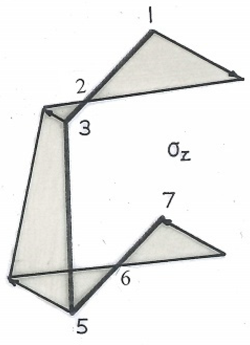
ꞷ1 = 0, (GJ/T)w1 = 0.2049d2 ꞷ2 = 0.1743d2, (GJ/T)w2 = 0.2049d2 − 0.1743d2 = 0.0306d2 ꞷ3 = 0.2988d2, (GJ/T)w3 = 0.2049d2 − 0.2988d2 = −0.0939d2 ꞷ4 = 0.21884d2, (GJ/T)w3 = 0.2049d2 − 0.2188d2 = −0.0139d2 ꞷ5 = 0.1616d2, (GJ/T)w3 = 0.2049d2 − 0.1616d2 = 0.0433d2 ꞷ6 = 0.1760d2, (GJ/T)w3 = 0.2049d2 − 0.1760d2 = 0.0289d2 ꞷ7 = 0.2306d2, (GJ/T)w3 = 0.2049d2 − 0.2306d2 = −0.0257d2

The warping distribution, w₁–w₇, is shown in Figure 16. Both positive and negative apply within the linear connections between each limb. The physical displacement, w, is found by multiplying each normalised ordinate ꞷ₁–ꞷ₄, as calculated above, by Td²/GJ.

Where one end is constrained these displacements are completely constrained to induce axial stress σ_z proportionately. This stress, which diminishes with the length to attain zero at the free end, depends upon the primary warping constant for the section, which is found from

Γ₁ = ∫_s ꞷ²tds − ϖ² ∫_s t ds

(22)

With t constant, the first integral in Equation (22) is found from the square of each line equation in Figure 15.

$$\begin{array}{l}1–3: t{\int }_s{ꞷ}^2\mathrm{d}s = t{\int }_0^{d/3}(0.8966ds{)}^2\mathrm{d}s = 0.8039d^{2}t\mid s^3/3{\mid }_0^{d/3}=0.009925d^{5}t\\ 3–5:t{\int }_s{ꞷ}^2\mathrm{d}s = t{\int }_{d/3}^{4d/3}(0.3447d^2-0.1373ds{)}^2\mathrm{ds}\\ = t{\int }_{d/3}^{4d/3}(0.1182d^4-0.09466d^{3}s+0.01885d^2{s}^2)\mathrm{ds}\\ = t\mid 0.1182d^{4}s -0.04733d^3{s}^2 + 0.006284d^2{s}^3 {\mid }_{d/3}^{4d/3}\\ =t(0.08835d^5-0.03437d^5)=0.05398d^{5}t\\ 5–7: t{\int }_s{ꞷ}^2\mathrm{d}s = t{\int }_{d/3}^{2d}(0.0236d^2+0.1035ds{)}^2\mathrm{ds}\\ = t{\int }_{4d/3}^{2d}(0.000557d^4+0.004885d^{3}s+0.01071d^2{s}^2)\mathrm{ds}\\ = t\mid 0.000557d^{4}s + 0.002443d^3{s}^2 + 0.00357d^2{s}^3 {\mid }_{4d/3}^{2d}\\ =t(0.03945d^5-0.01355d^5)=0.025904d^{5}t\end{array}$$

Substituting these into Equation (22) with ϖ and ∫t ds = t(2d) within the second term:

Γ1 = (0.009925d5t + 0.05398d5t + 0.025904d5t) − (0.2049d2)2t(2d) = (0.089809 − 0.083968) d5t = 0.00584d5t

The length coefficient μ follows:

μ = √(GJ/EΓ₁) = √(3J/8Γ₁) = 6.5428t/d²

in which E = 2G(1 + ν) = 8G/3 for ν = 1/3 and J = 2dt³/3. Then, μL = 6.5428(t/d)(L/d) = 1.7172 and exp(−2 μL) = 0.03225. These constants provide the axial stress, from constrained warping at the fixing, as

σ_z = −(ꞷ − ϖ)T/μΓ₁ × (1 − e^−2μL)∕(1 + e^−2μL)

(23a)

Equation (23a) is applied in a convenient form to the end section’s median points 1, 2, 3 … 7 as follows:

(d3t2/T)σz = 24.536 (ϖ − ꞷ)	(23b)
= 24.536 (0.2049d2 − ꞷ)

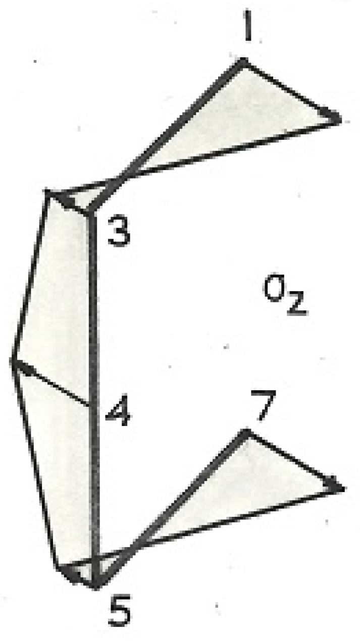
ꞷ1 = 0, (d3t2/T)σz1 = 5.027d2 ꞷ2 = 0.1743d2, (d3t2/T)σz2 = 24.536(0.2049d2 − 0.1743d2) = 0.751d2 ꞷ3 = 0.2988d2, (d3t2/T)σz3 = 24.536(0.2049d2 − 0.2988d2) = −2.304d2 ꞷ4 = 0.2188d2, (d3t2/T)σz4 = 24.536(0.2049d2 − 0.2188d2) = −0.341d2 ꞷ5 = 0.1616d2, (d3t2/T)σz5 = 24.536(0.2049d2 − 0.1616d2) = 1.062d2 ꞷ6 = 0.1760d2, (d3t2/T)σz3 = 24.536(0.2049d2 − 0.1760d2) = 0.709d2 ꞷ7 = 0.2306d2, (d3t2/T)σz7 = 24.536(0.2049d2 − 0.2306d2) = −0.631d2

The corresponding constrained axial stress distribution, σ_z, in Figure 17 is proportional to the unconstrained warping displacement (see Figure 16). Linear variations between tension and compression apply to each limb. A conversion of each ordinate (d³t²/T)σ_z into stress requires a multiplication factor, T/d³t², so that for median point 3, for example, Equation (23b) yields

σ_z3 = −2.304d² × T/d³t² = −2.304T/dt²

which, for a unit torque (T = 1 N m), a maximum elastic compressive stress is seen to occur at point 3 in the fixed-end cross-section:

σ_z3 = −2.304 × 1000∕[(25.4)³ × 15/8 × (3/64)²] = −34.13 MPa

The greatest tensile stress applies to point 1. This converts to σ_z1 = 74.47 MPa, which is also elastic under the stated torque.

The constrained axial stress, σ_z, in the beam diminishes with the length according to the first term in Equation (3a). This shows that a multiplication factor, K, applied to the fixed-end stresses provides the reduced stresses at length position 0 ≤ z ≤ L:

K = sinh μ(L − z)∕sinh μL = (e^−μz − e^{−μ(2L − z)})∕(1 − e^−2μL)

(23c)

For example, at half-length in this section, where z = L/2, Equation (23c) provides K = σ_z/σ_zo as

K = (0.4338 − 0.07609)∕(1 − 0.03225) = 0.527

where the central stress distribution is found by applying K to stress at the fixing, listed above.

9.6. Torsional Shear Flow

The corresponding torsional shear flow (see Section 2) is found from applying Equation (5b) to the swept area diagram as follows:

q = Etd³θ/dz³ × Q

(24a)

where

Q = ∫_s (ꞷ − ϖ) ds

(24b)

The integration for Q in Equation (24b) gives the change in the shear flow between points

$$\begin{array}{l}1–3: ꞷ-\varpi = 0.8966ds - 0.2049d^2\\ Q_{1-3} = {\int }_0^{d/3}(0.8966ds -0.2049d^2) \mathrm{d}s\\ = |0.4483d{s}^2- 0.2049d^{2}s {|}_0^{d/3} = 0.0498d^3 - 0.0683d^3 = -0.0185d^3\\ 3–5: ꞷ - \varpi = 0.3447d^2 -0.1373ds - 0.2049d^2 =0.1398d^2 -0.1373ds\\ Q_{3–5}={\int }_{d/3}^{4d/3}(0.1398d^2 - 0.1373ds) \mathrm{d}s = | 0.1398d^{2}s - 0.06865d{s}^2{|}_{d/3}^{4d/3}\\ =(0.1864d^3 - 0.12204d^3) - (0.0466d^3 - 0.00763d^3) = 0.02539d^3\\ 5–7: ꞷ - \varpi = 0.0236d^2 + 0.1035ds - 0.2049d^2=-0.1813d^2 + 0.1035ds\\ Q_{5–7} = {\int }_{4d/3}^{2d}(-0.1813d^2 + 0.1035ds) \mathrm{ds} = | -0.1813d^{2}s + 0.05175d{s}^2{|}_{4d/3}^{2d}\\ = (-0.3626d^3 + 0.2070d^3) - (-0.2417d^3 + 0.0920d^3) = -0.0059d^3\end{array}$$

Intermediate positions are taken to find the shape of the shear flow distribution between points 3 and 4 and 5 and 6 more accurately as follows:

$$\begin{array}{l}1–2:Q_{1–2}={|0.4483d{s}^2-0.2049d^{2}s|}_0^{7d/36}=0.01695d^3-0.03984d^3=-0.0229d^3\\ 3–4:Q_{3–4}={|0.1398d^{2}s-0.06865d{s}^2|}_{d/3}^{11d/12}\\ = (0.1282d^3-0.05769d^3)-(0.0466d^3-0.00763d^3)=0.03154d^3\\ 5–6:Q_{5–6}={|-0.1813d^{2}s+0.05175d{s}^2|}_{4d/3}^{53d/36}\\ = (-0.2669d^3+0.1122d^3)-(-0.2417d^3+0.092d^3)=-0.005d^3\end{array}$$

Between 3 and 5, a maximum Q applies, when

$$\begin{array}{l}\mathrm{d} (0.1398d^{2}s -0.06865d{s}^2)/\mathrm{d}s=0\\ 0.1398d^{2-}-0.1373ds=0\\ s=1.018d\\ \therefore Q_{\mathit{max}}={|0.1398d^{2}s-0.06865d{s}^2|}_{d/3}^{1.018d}\\ = (0.1424d^3-0.0712d^3)-(0.0466d^3-0.00763d^3)=0.03186d^3\end{array}$$

The shear flow changes calculated above for each limb are connected along a horizontal median line in Figure 18a. They reveal, correctly, that net shear flow for the median line 1, 2, 3 … 7 has zero value for end points 1 and 7. Each net shear flow measure Q/d³ at these points is plotted upon the channel section in Figure 18b.

The conversion to q (N/mm) from Equation (24a) applies q = Et d³θ/dz³ × Q. For example, at point 3 within the fixed-end cross-section, Figure 18b shows Q = −0.0185d³, which is converted to q for a unit torque of 1 Nm applied to section C, with d = 1⅞″, as follows:

q = Et d³θ/dz³ × Q

At the fixing where z = 0, the third derivative in Equation (6c) is reduced to

d3θ/dz3 = −(μ2T/JG) = −T/EΓ1 ∴ q = −Tt/Γ1 × Q = (−Tt/0.00584d5t) × (−0.0185d3) = 3.1678T/d2 = (3.1678 × 1000)/(1.875 × 25.4)2 = 1.398 N/mm

Note the sign change that appears for q. Here, a full conversion from Q to q reverses the distribution given in Figure 18b. Equation (6c) is required in full when conversions are applied to intermediate span positions z = L/4, L/2, etc. (see Table 1).

Variation in the torsional stiffness with the length follows from the twist rate [1]:

dθ/dz = (T/GJ) [1 − coshμ(L − z)∕coshμL]

Integrating for θ,

θ = (T/GJ) [z + sinhμ(L − z)∕μcoshμL] + C

where C = −(T/GJ)(sinhμL)∕(μcoshμL), is required to provide zero twist at the fixed end (z = 0). Hence,

θ = (T/GJ) [z + sinhμ(L − z)∕μcoshμL] − (T/GJ)(sinhμL)∕(μcoshμL)	(25a)
= (T/GJ){z + [sinhμ(L − z) − sinhμL]∕μcoshμL}

Stiffness T/θ at position z is found from Equation (25a):

T/θ = GJ∕{z + [sinhμ(L − z) − sinhμL]∕μcoshμL}

(25b)

For example, at the first quarter position z = L/4, substituting μL = 1.7172 for L = 500 mm, G = 70 × 10³ MPa and J = 53.588 mm⁴, found previously, into Equation (25b) provides the following:

T/θ = GJ∕{L/4 + [sinh(3 μL/4) − sinhμL]∕μcoshμL} = (70 × 103 × 53.588)∕[125 + (1.675 − 2.695)∕(0.003434 × 2.874] = 173.27 × 103 N mm/c = 173.27 N m/c

For z = L/2:

T/θ = GJ∕{L/2 + [sinh(μL/2) − sinhμL]∕μcoshμL} = (70 × 103 × 53.588)∕[250 + (0.968 − 2.695)∕(0.003434 × 2.874)] = 50 × 103 N mm/c = 50 N m/c

For z = 3L/4:

T/θ = GJ∕{3L/4 + [sinh(μL/4) − sinhμL]∕μcoshμL} = (70 × 103 × 53.588)∕[375 + (0.4426 − 2.695)∕(0.003434 × 2.874)] = 25.56 × 103 N mm/c = 25.56 N m/c

For z = L

T/θ = GJ∕{L + [sinh(0) − sinhμL]∕μcoshμL} = (70 × 103 × 53.588)∕[500 + (0 − 2.695)∕(0.003434 × 2.874)] = 25.56 × 103 N mm/c = 16.53 N m/c

The variation in stiffness with length is shown in Figure 19. Stiffness is retained at all positions including the free end. All are seen to exceed St Venant’s unconstrained torsional stiffness [1]:

T/θ = JG/L = 53.588 × 70 × 10³/500 = 7.5 × 10³ N mm/^c = 7.5 N m/^c

9.7. Bending Stress Distribution

Referred the section’s principal centroidal axes (u and v), the axial stress in bending becomes

σ_z = M_x′y/I_x + M_y′x/I_y

(26a)

where M_x′ and M_y′ are equivalent moments expressed more conveniently in the centroidal axes (x and y). We integrate the equivalent shear forces given in Equation (18b,c) as

M_x′ = ∫F_y′dz = [M_x − M_y(I_xy/I_y)]∕[1 − (I_xy²/I_x I_y)]

(26b)

M_y′ = ∫F_x′dz = [M_y − M_x(I_xy/I_x)]∕[1 − (I_xy²/I_x I_y)]

(26c)

in which M_x and M_y are the applied moments at position z within the length:

M_x = F_y(L − z),

(27a)

M_y = F_x(L − z)

(27b)

Figure 20a shows the section of a cantilever of length L, free-end loaded with forces F_x and F_y applied at its centroid.

9.8. Trans-Moments

The trans-moments, which arise in the transfer of M_x and M_y from centroid G to shear centre E, are given as

B_x = M_x e_y

(28a)

B_y = M_y e_x

(28b)

where e_x and e_y are the perpendicular distances between rectangular axes x and y at G and E. Equation (28a,b) are taken to contribute, respectively, to the first and second terms in the axial stress Equation (26a):

σ_z1 = B_x/I_Ex = M_x E_y/I_Ex

(29a)

and

σ_z2 = B_y/I_Ey = M_y E_x/I_Ey

(29b)

Combining Equation (26a) with Equation (29a,b) gives the total axial stress from the two bending sources:

σ_z = [(M_x′y/)/I_x + (M_x E_y)/I_Ex] + [(M_y′x/)/I_x + (M_y E_x)/I_Ey]

(30a)

in which the parallel axis theorem provides for the change in I_x and I_y accompanying a separation between the respective parallel axes for G and E: (i) E_x = e_x + X’ between I_y and I_Ey and (ii) E_y = Y’−e_y between I_x and I_Ex (see Figure 20a,b)

I_Ex = I_x + AE_y²

(30b)

I_Ey = I_y + AE_x²

(30c)

in which A is the channel section area. To apply Equation (30a–c), recall that the following section properties are required:

X′ = 5d/36, Y′ = 5d/12, ex = 21d/153, ey = 9d/87, Ix = 17d3t/72, Iy = 87d3t/1944 and Ixy = −39d3t/648.

which provide the three ratios between second moments of area appearing in Equation (26b,c):

I_xy/I_x = −0.2549, I_xy/I_y = −1.3448, and I_xy²/I_x I_y = 0.3428

Initial calculations are made in the absence of trans-moments, substituting into Equation (26a,c):

σz = [Fy (500 − z)1.522 + Fx (500 − z)2.046] y∕0.2361d3t   + [Fx (500 − z)1.522 + Fy (500− z)0.3879] x∕0.04475d3t

(31a)

This shows that the greatest stress occurs at the fixing (z = 0) when Equation (31a) simplifies to

σz = (761 Fy + 1023 Fx)(y/d)∕0.2361d3t + (761 Fx + 193.95 Fy)(x/d)∕0.04475d3t σz d2t/103 = (3.223Fy + 4.333Fx)(y/d) + (17.005Fx + 4.334Fy)(x/d)

(31b)

with σ_z in MPa, d and t in mm. Equation (31b) is reduced for the following load combinations:

(1)

F_x = F; F_y = 0, |σ_z d²t/10³ = 4.333(y/d) + 17.005(x/d);

(2)

F_y = F; F_x = 0, |σ_z d²t/10³ = 3.223(y/d) + 4.334(x/d);

(3)

F_x = F_y = F, |σ_z d²t/10³ = 7.556(y/d) + 21.339(x/d);

(4)

F_x = −F; F_y = F, |σ_z d²t/10³ = −1.11(y/d) − 12.671(x/d).

Table 12. Asymmetric bending stress calculations for median line points 1, 2, 3 … 7 by Equations (1)–(4).

Point	1	2	3	4	5	6	7
x/d	7/36	0	−5/36	−5/36	−5/36	0	19/36
y/d	7/12	7/12	7/12	0	−5/12	−5/12	−5/12
Equation (1)	5.834	2.528	0.166	−2.362	−4.167	−1.805	7.169
σz/MPa	216.05	93.61	6.15	−87.47	−154.	−66.84	265.5
Equation (2)	2.723	1.88	1.278	−0.6019	−1.95	−1.343	0.9445
σz/MPa	100.83	69.62	47.32	−22.29	−72.02	−49.73	34.97
Equation (3)	8.557	4.408	1.444	−2.964	−6.112	−3.148	8.114
σz/MPa	316.9	163.2	53.5	−109.8	−226.3	−116.6	300.5
Equation (4)	−3.111	−2.464	1.112	1.76	2.222	0.4625	−6.225
σz/MPa	−115.2	−91.2	43.2	65.2	82.3	17.1	−230.5

is constructed for the axial stresses that apply to median points 1, 2, 3 … 7. The first two rows provide the co-ordinates of each point, which apply to each of (1)–(4) above.

Figure 21a–d shows the elastic bending stress distributions for the four load combinations where F = 100 N. With equal forces applied to G in the negative x and y directions, Figure 21c becomes the sum of the stresses with each of these forces applied separately (i.e., Figure 21a,b). When the direction of F_x is reversed, this has the effect of raising compression in each flange while lowering tension in the web (see Figure 21d). Linear stress distributions apply within each limb, but intersections giving zero stress do not correspond to ‘neutral axis’ points 2, 4 and 6 in Figure 20a.

In this author’s interpretation of trans-moment stress distributions, the four force combinations are treated separately and then superimposed in Figure 21a–d as required. By the parallel axis theorems, Equation (30b,c), the separation (see Figure 20a,b) between (i) the horizontal axes x (through G) and x_E (through E) is

E_y = Y′ − e_y = 5d/12 − 9d/87 = 0.3132d

(32a)

and (ii) the separation (see Figure 11b) between vertical axes y (through G) and y_E (through E) is

E_x = X′ + e_x = 5d/36 + 21d/153 = 0.2761d

(32b)

Applying Equation (30b,c),

I_Ex = I_x + AE_y² = 17d³t/72 + 2dt(0.3132d)² = 0.4323d³t

I_Ey = I_y + AE_x² = 87d³t/1944 + (2dt)(0.2761)² = 0.1972d³t

Separating the two trans-moment terms in Equation (30a), their summation at the fixing (z = 0) is

σz = (Mx Ey)/IEx + (My Ex)/IEy   = (Fy L)Ey/IEx + (Fx L)Ex/IEy

(33a)

We substitute for this section’s properties as given above

σz = FyL(0.3132d)∕(0.4323d3t) + FxL(0.2761d)∕(0.1972d3t)   = (0.7245Fy + 1.40Fx)L/(d3t)

(33b)

which reveals that σ_z is uniform for a given force combination. For example, taking case (3) above (F_x = F_y = F), Equation (33a) leads to

σ_z = 2.1245FL∕(d³t)

which, for F = 100 N, σ_z = 20.98 MPa, which is to be distributed to each stress level calculated under (3) in Table 12. This distribution is demonstrated for the simpler case of a symmetric channel section that follows.

9.9. Axial Symmetry

Finally, take the case of axially symmetric channel sections A–C, considered earlier. Because G and E both lie on the centroidal x-axis of symmetry, a single trans-moment refers to the shift in M_y from centroidal axis y to shear centre axis y_E, i.e., through a perpendicular distance, E_x = e_x + X′. There is no shift in M_x along the centroidal axis. Therefore, from Equation (30b,c),

σ_z = M_y E_x/I_Ey where I_Ey = I_y + AE_x²

Applied to the symmetrical channel section in Figure 1a, for example, with F_x = 100 N, the uniform axial stress that arises from the trans-moment is found:

E_x = e_x + X′ = 3a/8 + a/4 = 5a/8

IEy = (3.28 × 10−3)d4 + (2dt)(5a/8)2 IEy/d4 = (3.28 × 10−3) + 2(t/d)(5/8)2(a/d)2 = (3.28 × 10−3) + 2(1/16)(5/8)2(1/2)2 = 0.01548 ∴ IEy = 0.01548d4 = 6446.2 mm4

σ_z = (M_y E_x)/I_Ey = (F × 300)(5/8 × 12.7)∕6446.2 = 36.9 MPa

(34a)

which is distributed to each median point in proportion to its x-co-ordinate by two methods:

(i) From Equation (34a), the stress adjustments to be applied to Table 12 are as follows:

σz1 = σz7 = (a − X′)σz∕(ex + X′)    = (a − a/4)σz∕(3a/8 + a/4) = 6σz/5 = 6 × 36.9/5 = + 44.28 MPa σz2 = σz6 = 0 σz3 = σz4 = σz5 = −X′ σz∕(ex + X′)    = −(a/4)σz∕(3a/8 + a/4) = −2σz/5 = −14.76 MPa

(ii) In another interpretation of the trans-moment’s conversion to bending stress, the moment arm is increased from L to L + E_x, giving M_y = F_x(L + E_x):

σ_z = (M_y E_x)∕I_Ey = F_x(L + E_x)x_i∕I_Ey

(34b)

Here, M_y is referred to axis y_E where the parallel axis theorem has been applied to give I_Ey and where x_i represents the x-co-ordinates for median points i = 1, 2, 3 … 7. Applying Equation (34b) to symmetrical channel section A yields the following:

σz1 = σz7 = 100 × (300 + 5a/8)(a − a/4)/6446.2    = 100 × 307.94 × 9.525/6446.2 = +45.5 MPa      σz2 = σz6 = 0 σz3 = σz4 = σz5 = 100 × (300 + 5a/8)(−a/4)/6446.2    = 100 × 307.94 × (−3.175)/6446.2 = −15.17 MPa

Numerically, with these adjustments, method (ii) in reasonable agreement with the method (i).

10. Conclusions

The stress analysis of a thin-walled, cantilever beam with open channel sections shows that this is by no means a simple structure. With transverse end loading applied to a symmetric channel’s centroid in alignment with its principal directions, the beam bending theory is supplemented by the influence of torsion and flexural shear applied to the shear centre. Thus, in beam design, the maximum net axial stress and maximum net shear stress are found at the fixing. These apply to the application of yield criteria in the assessment of the beam’s safe load bearing capacity. Given that torque Equation (4) depends linearly upon F_x the latter may be reduced to lower the shear stress to acceptable levels where necessary. However, a load factor should not be applied until the additive effect of bending upon the net axial stress distribution has been established.

Further information provided by the sophisticated Wagner–Vlasov theory is illustrated well for a thin-walled, non-symmetrical channel. Following all the necessary geometric calculations that appear as the symbols X′, Y′, I_x, I_y, I_xy, ϖ, Γ₁, J and μ for this particular cross-section, the logical sequence of calculations when transverse forces are applied to the centroid at the free-end of a cantilever beam is as follows:

(1)

Establish the flexural shear flow distribution with equivalent forces for the principal axes transferred to the shear centre.

(2)

Calculate the unconstrained warping displacements for the resultant St. Venant torque, arising from the transfer in (1), applied to the shear centre.

(3)

Calculate the axial stress produced by the Wagner torque arising from constraining warping by fixing one end.

(4)

Calculate the torsional shear flow arising from the Wagner torque in (3).

(5)

Assess the increased torsional stiffness at length positions arising from (3).

(6)

Find the net shear flow (stress) distribution from the addition of (1) and (4). Note the stress gradient across the thickness with (1) providing the mean stress and (4) the superimposed linear distribution due to torsion.

(7)

Find the bending stress distribution from equivalent moments referred to the principal axes with end forces applied at the centroid.

(8)

Find the net axial stress distribution from the addition of (3) and (7).

(9)

Apply criteria of yielding/buckling [16,17,18,19,20] to fixed-end positions stressed most severely under (6) and (8).

The possibility of a transfer in moments accompanying the shift in forces from G to E has been quantified for both types channel. The conversion to bending stress shows this how influence can augment the net bending stress in consideration of plastic collapse arising at median perimeter points for each section.

References

- Rees, D.W.A.; Al-Sheikh, A.M.S. Theory of flexural shear, bending and torsion for a thin-walled beam of open section longitudinal axis of loading thin-walled beams of open section. World J. Mech. 2024, 14, 23–53. [Google Scholar] [CrossRef]
- ESDU 78020; Local Buckling and Crippling of I, Z and Channel Section Struts. National Technical Reports Library: Alexandria, VA, USA, 1978.
- Nix, W.D. Mechanical properties of thin films. Metall. Trans. A 1989, 20, 2217–2245. [Google Scholar] [CrossRef]
- Zou, M.; Ma, Y.; Yuan, X.; Hu, Y.; Liu, J.; Jin, Z. Flexible devices: From materials, architectures to applications. J. Semicond. 2018, 39, 011010. [Google Scholar] [CrossRef]
- Papangelis, J. On the stresses in thin-walled channels under torsion. Buildings 2024, 14, 3533. [Google Scholar] [CrossRef]
- Yu, Y.; Wei, H.; Zheng, B.; Tian, D.; He, I. Integrated dynamic analysis of thin-walled beams coupled bi-directional loading, torsion and axial vibration under axial loads. Appl. Sci. 2024, 14, 11390. [Google Scholar] [CrossRef]
- Vlasov, V.Z. Thin-Walled Elastic Beams; Oldbourne Press: London, UK, 1961. [Google Scholar]
- Baigent, A.H.; Hancock, G.J. Structural analysis of assemblages of thin-walled members. Eng. Struct. 1982, 4, 207–216. [Google Scholar] [CrossRef]
- Boresi, A.P.; Schmidt, R.J.; Sidebottom, O.M. Advanced Mechanics of Materials, 2nd ed.; Wiley: Hoboken, NJ, USA, 1993. [Google Scholar]
- Wagner, H. Torsion and Buckling of Open Sections; No. NACA-TM-807; NTRS-NASA: Washington, DC, USA, 1936. [Google Scholar]
- Oden, J.T.; Ripperger, E.A. Mechanics of Elastic Structures, 2nd ed.; McGraw-Hill: New York, NY, USA, 1980. [Google Scholar]
- Cook, R.D.; Young, W.C. Advanced Mechanics of Materials, 2nd ed.; Prentice-Hall: Hoboken, NJ, USA, 1998. [Google Scholar]
- Gao, Z.H. A unified theory of thin-walled structures. J. Struct. Mech. 1981, 9, 179–197. [Google Scholar]
- Vetyuko, Y. Direct Approach to Elastic Deformation and Stability of Rods of Open Profile; Springer: Berlin/Heidelberg, Germany, 2008. [Google Scholar]
- Gjelsvik, A. Theory of Thin-Walled Beams; John Wiley and Sons: Hoboken, NJ, USA, 1981. [Google Scholar]
- Bleich, F.; Bleich, H.H. Buckling Strength of Metal Structures; McGraw-Hill: New York, NY, USA, 1952. [Google Scholar]
- Hoff, N.J. The effect of the edge conditions on the buckling of thin-walled circular cylindrical shells in axial compression. In Applied Mechanics; Görtler, H., Ed.; Springer: Berlin/Heidelberg, Germany, 1966. [Google Scholar] [CrossRef]
- Drillenberg, M. Torsion and Shear Stresses Due to Shear Centre Eccentricity; SCIA 2017; Delft University of Technology: Delft, The Netherlands, 2017. [Google Scholar]
- Wen, Y.L.; Kuo, M.H. General expression for the torsional warping of a thin-walled open section beam. Int. J. Mech. Sci. 2003, 43, 830–849. [Google Scholar]
- Wang, G. Restrained torsion of open thin-walled beams including shear deformation effects. J. Zhejiang Univ. Sci. 2012, A13, 260–273. [Google Scholar] [CrossRef]