Article

Analyzing and Forecasting Vessel Traffic Through the Panama Canal: A Comparative Study

by
Mitzi Cubilla-Montilla
1,2,*,
Anabel Ramírez
1,
William Escudero
3 and
Clara Cruz
1
1
Departamento de Estadística, Facultad de Ciencias Naturales, Exactas y Tecnología, Universidad de Panamá, Panama City 0824, Panama
2
Sistema Nacional de Investigación de Panamá (SNI), Secretaría Nacional de Ciencia, Tecnología e Innovación (SENACYT), Panama City 0816, Panama
3
Independent Researcher, Panama City 0824, Panama
*
Author to whom correspondence should be addressed.
Appl. Sci. 2025, 15(15), 8389; https://doi.org/10.3390/app15158389
Submission received: 19 June 2025 / Revised: 24 July 2025 / Accepted: 24 July 2025 / Published: 29 July 2025

Abstract

The Panama Canal, inaugurated in 1914, continues to play a pivotal role in global maritime connectivity. In 2016, the Canal underwent a significant expansion, reshaping maritime transit by accommodating larger vessels and reinforcing its strategic importance in international trade. The objective of this study is to identify a suitable time series statistical model to forecast the number of vessels transiting the Panama Canal. The three approaches employed were the following: the Autoregressive Integrated Moving Average (ARIMA) model, the Holt–Winters (HW) exponential smoothing method, and the Neural Network Autoregressive (NNAR) model. The models were compared based on forecasting errors to evaluate their predictive accuracy. Overall, the NNAR model exhibited slightly better predictive performance than the SARIMA (1,0,1) (0,1,1) model in terms of error, with both outperforming the Holt–Winters model by a significant margin.

1. Introduction

Panama is a country located in Central America, whose economy relies heavily on port and logistics activities. The Panama Canal, strategically positioned at the narrowest point between the Atlantic and Pacific Oceans, serves as the primary route enabling rapid interoceanic communication in the Western Hemisphere. It plays a key role in the country’s growth and development [1] as well as in international trade [2,3].
Since its inauguration on 15 August 1914, the Canal’s high-capacity maritime infrastructure has had a significant global impact by reducing distances and maritime communication times [4,5]. By enabling shorter shipping routes, the Panama Canal contributes to efforts aimed at reducing the carbon footprint of maritime transport, as it significantly lowers fuel consumption and CO2 emissions. This reinforces its role not only as a vital economic infrastructure, but also as a tool for advancing sustainable maritime transportation. The Canal’s infrastructure has driven major economic and commercial advancements that have endured for over a century.
In 2016, the expansion of the Panama Canal was completed—a project that included the construction of new locks capable of accommodating larger vessels with greater draft. This development reflects a broader trend in the maritime industry toward achieving economies of scale through the use of larger ships, known as Neopanamax vessels, thereby enhancing global maritime transport capacity [6].
Indeed, the Interoceanic Waterway is utilized by approximately 180 maritime routes, connecting 1920 ports across 170 countries [7]. The principal types of cargo transported through the Canal include grains, containerized goods, petroleum and its derivatives, vehicle carriers, and cruise liners [8]. Most of the Canal traffic flows between the Atlantic coast of the United States and the Far East, while trade between Europe and the western coasts of the United States and Canada represents the second most significant route. However, other regions—particularly neighboring countries in Central and South America—are proportionally more dependent on this vital artery to support their economic development and expand trade.
In fiscal year 2024, the Panama Canal recorded a total of 11,240 transits by both large and small commercial vessels, which transported 210 million long tons of cargo and generated toll revenues amounting to USD 3.381 billion [9]. Undoubtedly, the number of vessels transiting the Panama Canal has increased following its expansion and is closely linked to financial indicators and the economic activities of transportation, communication, logistics, trade, and tourism.
In this context, maritime transport has gained increasing relevance in recent years, fostering growing interest in enhancing the operational efficiency of navigable waterways [10]. Accordingly, the analysis of vessel traffic through the Panama Canal, together with the development of predictive models, has emerged as a critical tool for anticipating demand and informing strategic decision-making.
The scientific literature includes numerous studies employing forecasting methods across various fields [11,12,13,14,15]. However, forecasting vessel traffic represents a particular challenge due to the inherent complexity of its behavior, which is multifactorial in nature. This type of traffic is influenced by a variety of operational and structural factors, such as the vessel type, industrial production levels, characteristics of logistics operations, and specific configuration of each port, among others [16]. Nevertheless, as long as a well-compiled historical series is available and an appropriate forecasting model is used, the results can be considered reliable.
Historically, maritime traffic forecasting has primarily relied on conventional statistical methods, given their effectiveness in capturing linear and seasonal patterns in time series. In this regard, the study by Ref. [17] applied the ARIMA model to predict the monthly volume of maritime traffic at the port of Incheon, South Korea. Their findings showed that this model outperformed the exponential smoothing method by more accurately capturing the seasonal variations in vessel traffic. Similarly, Ref. [18] employed the SARIMA model to analyze the time series of maritime traffic flow at the port of Jingzhou, demonstrating that this model adequately represents the seasonality present in the monthly vessel flow.
In recent years, modern approaches based on neural networks and deep learning techniques have been adopted, allowing for the modeling of nonlinear [19] and complex dynamic relationships, thereby improving forecasting accuracy across various fields. Unlike traditional statistical models, which assume linear relationships, the NNAR is capable of capturing nonlinear patterns present in the data, such as seasonal fluctuations, trends, meteorological phenomena, and irregular global-scale behaviors. For example, Ref. [20] validated the use of artificial neural networks as a complementary approach to classical models in maritime traffic forecasting. Along the same lines, Ref. [16] implemented seasonal SARIMA models and neural networks to forecast container ship traffic between 2020 and 2025 at the port of Rajaee, Iran’s largest port, concluding that neural networks provided superior predictive performance compared to the SARIMA approach. Likewise, Ref. [21] analyzed the maritime cargo traffic series in Spanish ports between 1997 and 2017, employing both linear and nonlinear univariate models, such as SARIMA, exponential smoothing, and neural networks. Based on their results, the authors concluded that prediction accuracy varies depending on the type of cargo transported, with linear models generally outperforming nonlinear ones. Furthermore, Ref. [22] proposed a hybrid approach combining empirical mode decomposition with traditional neural networks to predict high- and low-frequency components in maritime traffic time series. In the same vein, Ref. [23] applied neural networks to forecast monthly traffic in the Suez Canal, achieving greater accuracy than ARIMA models. Similarly, Ref. [24] implemented artificial intelligence models, specifically neural networks, to estimate maritime traffic, tackling the complexity of flow data in ports and the challenge of capturing dynamic spatiotemporal dependencies.
In a recent advancement, Ref. [25] proposed a dynamic spatiotemporal model called the Temporal Convolutional Network–Bidirectional Gated Recurrent Unit–Pearson Correlation Coefficient–Graph Attention Network (TG-PGAT), specifically designed to address the complexity of maritime traffic flow in ports. This model demonstrated greater prediction accuracy and stability compared to other classical forecasting methods used in this field.
Despite advancements in maritime traffic forecasting, most studies have concentrated on ports and shipping lanes outside the interoceanic context of the Panama Canal. Given the strategic significance of this waterway at both regional and global levels, this article aims to identify a statistical time series model capable of accurately forecasting the number of vessels transiting the Panama Canal. To date, no prior research has been found that applies time series methodologies to model vessel traffic through the Panama Canal—except for the work of Timoshenkova et al. [26]. To address this, a comparison is proposed between traditional techniques—such as the seasonal SARIMA model and the Holt–Winters method—and artificial intelligence-based models, such as Neural Network Autoregressive (NNAR) models. This integration responds to the need to assess whether classical approaches, widely used for their interpretability and effectiveness in linear contexts, can be outperformed or complemented by more recent techniques capable of capturing nonlinear dynamics and complex patterns in the data.
Accordingly, this study contributes to the literature by providing a comprehensive statistical analysis of the historical series of vessel transits through this maritime route, thereby helping to expand the limited body of scientific research on vessel traffic through the Panama Canal. Furthermore, it lays the groundwork for future research in this area. The results show that both the SARIMA and NNAR models exhibit superior predictive performance and better statistical fit compared to the Holt–Winters model for forecasting vessel traffic through the Panama Canal.

2. Materials and Methods

2.1. Data Description

Data on the number of vessels transiting the Panama Canal were obtained from the Annual Reports published by the Panama Canal Commission [27], Panama Canal Authority [8], and National Institute of Statistics and Census of the Office of the Comptroller General of the Republic of Panama [28].
The dataset used has a monthly frequency, corresponding to vessel transit data through the Panama Canal over a 23-year period, from January 2000 to December 2022, totaling 276 observations.
Ships navigating the Panama Canal follow a maritime route connecting the Caribbean Sea with the Pacific Ocean, crossing the narrowest section of the Isthmus of Panama (Figure 1).

2.2. Methodology

This study employed three approaches to model and forecast vessel traffic through the Panama Canal: the Autoregressive Integrated Moving Average (ARIMA) model, the Holt–Winters (HW) method, and the Neural Network Autoregressive (NNAR) model. According to Mgale [29], these models can predict time series data exhibiting seasonal patterns. The methods considered in this manuscript were selected because the SARIMA, Holt–Winters, and NNAR models all generate forecasts based solely on past values of the time series, without requiring exogenous variables. This choice ensures a fair comparison among the approaches, as all models operate from the same informational basis. Additionally, given the challenge of precisely identifying linear and nonlinear patterns in the vessel traffic time series through the Panama Canal, these three methods were applied. It is worth noting that there is no consensus technique among researchers for forecasting in contexts related to navigable waterways
To develop and fit the models, the time series was split into two subsets: 80% of the observations were allocated to the training set, and the remaining 20%, to the testing set. The training set was used for parameter estimation and model construction, while the testing set served to evaluate predictive performance.
The metrics employed to assess model performance included RMSE, MPE, MAE, and MAPE. Subsequently, the models were used to forecast the number of vessels transiting the Panama Canal from January to December 2023.
The time series analysis was conducted using the R programming language [30], supported by the integrated development environment RStudio [31], version 4.2.1.

2.2.1. Autoregressive Integrated Moving Average (ARIMA)

In univariate ARIMA models, the behavior of a time series is explained based on its past or lagged observations [32] and stochastic error terms. This model integrates three components, Autoregressive (AR), Integration (I), and Moving Average (MA), each characterized by specific parameters: p denotes the number of autoregressive parameters (AR), d is the number of differencing steps needed to make the series stationary (I), and q is the number of moving average parameters (MA).
Thus, the model is denoted as ARIMA (p, d, q). Mathematically, the model can be expressed by the following equation:
X t = μ + X t 1 + X t d + + ϕ 1 X t 1 + ϕ 2 X t 2 + + ϕ p X t p + e t ϕ 1 e t 1 ϕ 2 e t 2 ϕ q e t q
If the ARIMA model incorporates a seasonal component, it can be represented as S A R I M A   p ,   d ,   q ( P ,   D ,   Q ) , where the first parentheses (p, d, q) correspond to the non-seasonal autoregressive process, and the second parentheses (P, D, Q) denote the seasonal variation in the time series. Thus, SARIMA is essentially an extension of ARIMA used when a seasonal pattern is evident in the time series [33].
Mathematically, the model is expressed by the following equation [34]:
1 B 1 B 12 1 ϕ 12 B 12 y t = μ + 1 + θ 1 B + θ 2 B 2 + θ 3 B 3 + π 1 B 12 + π 2 B 24 e t
Box and Jenkins [35,36] is the most widely used statistical procedure for analyzing and interpreting time series data in order to develop forecasting models such as ARIMA and SARIMA. Essentially, it involves identifying a mathematical model that represents the behavior of a time series and enables forecasting for a given time period. This methodology is divided into four stages [37]. The first stage, identification, involves recognizing patterns of trend, seasonality, and periodicity, and transforming the series into a stationary one. The next stage, estimation, consists of plotting the simple and partial correlograms to identify parameters based on the simple and partial autocorrelations. The third phase, validation, entails assessing the model fit through residual analysis and the Ljung–Box test. Finally, the forecasting stage involves generating predictions based on the selected and validated models. The entire process is summarized in the following flowchart (Figure 2).

2.2.2. Holt–Winters Method

During the validation stage, ARIMA/SARIMA models can be compared with alternative methodologies capable of making predictions from seasonal data [38]. One such alternative is the Holt–Winters method [39]. This approach typically assumes that the series can be decomposed into some or all of the following components: (a) trend, (b) cyclical, (c) seasonality, and (d) irregular [40]. Furthermore, the model structure can be either additive or multiplicative, depending on the nature of the seasonality [41].
The application of this method is based on a theoretical model used for forecasting, expressed as the following:
Y t = b 0 + b 1   E t +   μ t
where b o is the level component, b 1 is the slope of the trend line, and E t represents the multiplicative seasonal factor.
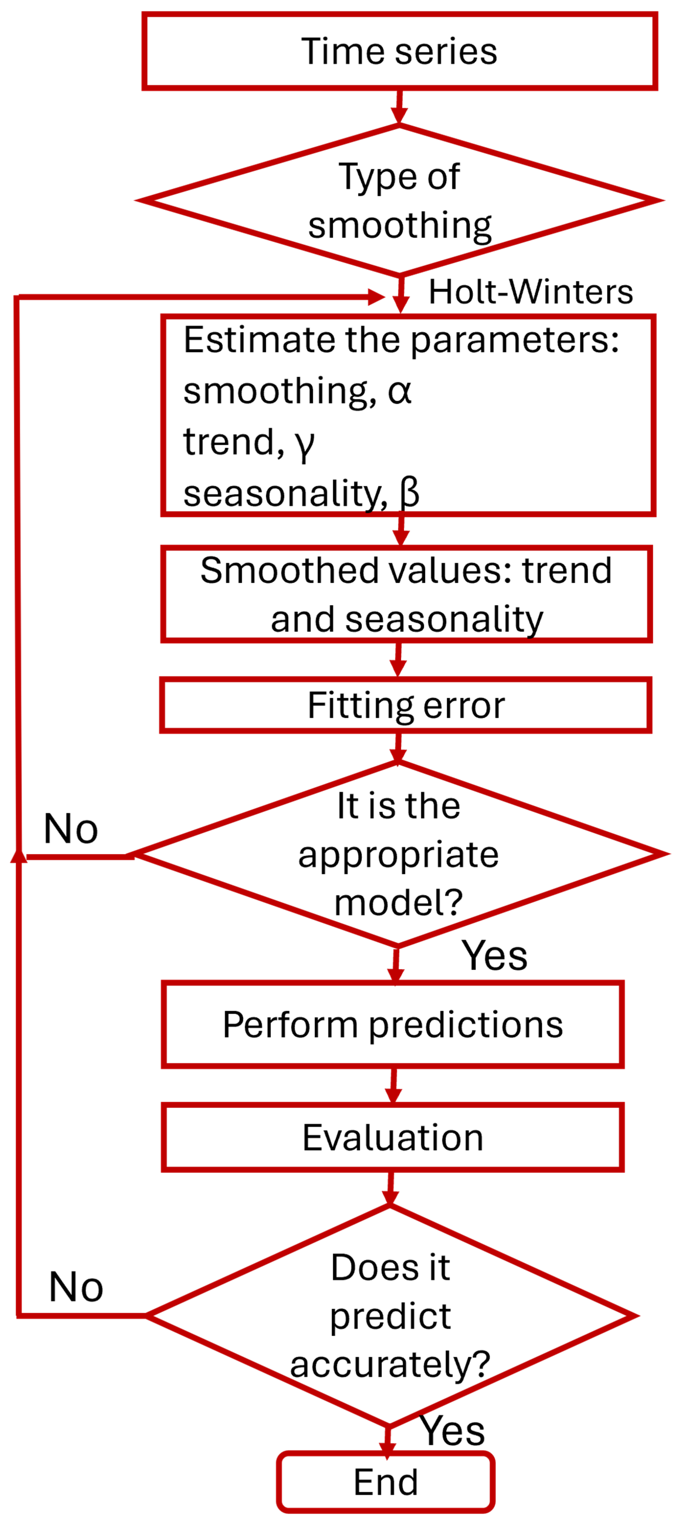
The process begins with the initialization of these components based on historical data. Then, at each period, the level, trend, and seasonality are iteratively updated using smoothing formulas that incorporate the parameters α, β, and γ. Finally, the model combines these components to generate forecasts that reflect both the overall evolution and the seasonal patterns of the time series. The following flowchart (Figure 3) details these steps, showing how the sequential updating of each component is performed to optimize forecast accuracy.

2.2.3. Neural Network Autoregressive (NNAR)

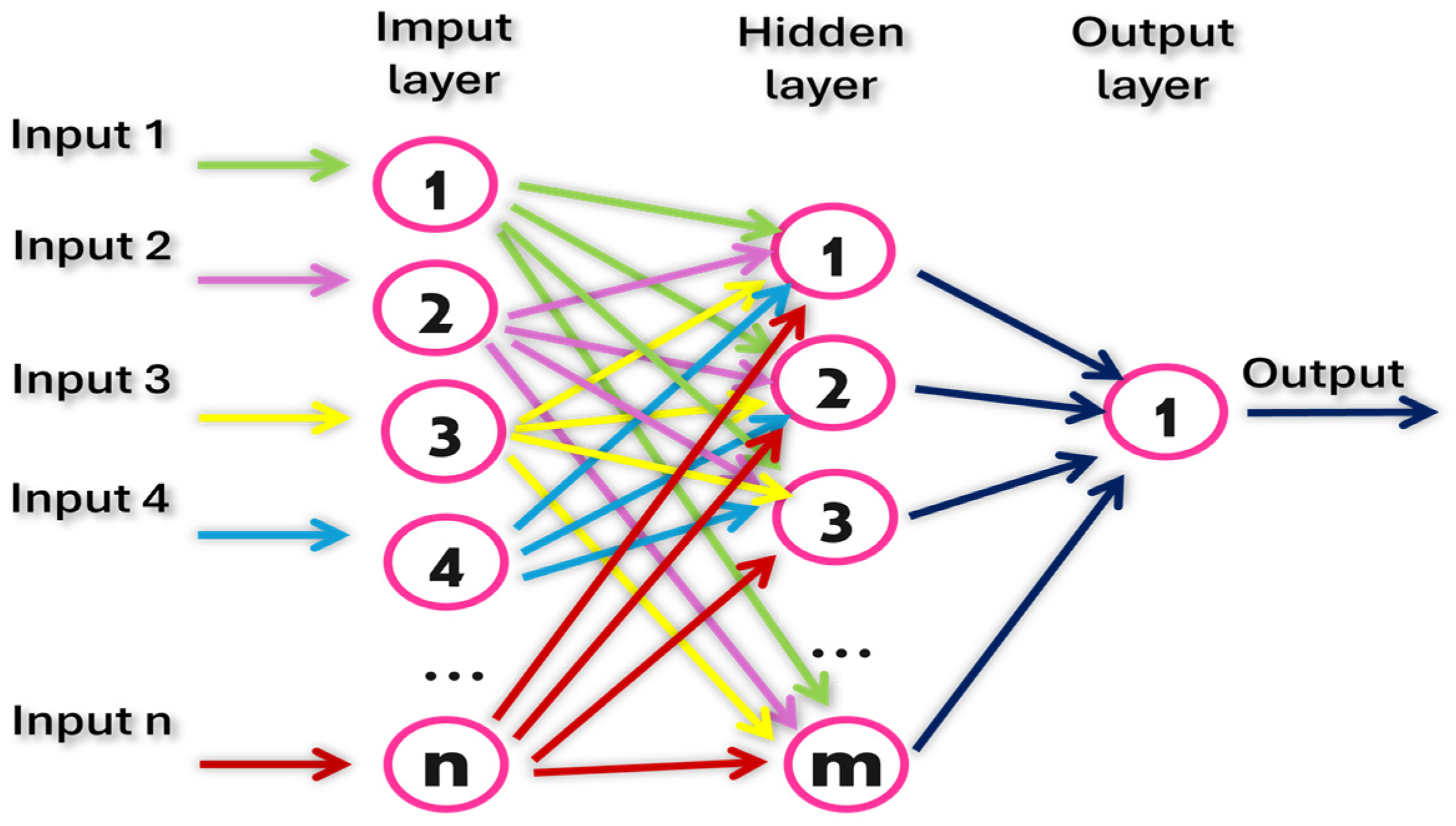
Artificial neural networks, based on a mathematical model that mimics brain function, are widely used in time series modeling and forecasting [15]. Their fundamental architecture consists of an input layer, one or more hidden layers, and an output layer. The input layer receives the initial data, while the hidden layers process this information through weighted connections and activation functions to detect complex patterns. Finally, the output layer generates the network’s prediction or output. This structure enables the network to learn and model nonlinear relationships within the data [42]. Once a neural network has been trained, it can be used to predict outputs for new inputs that have not been seen before. The following figure (Figure 4) presents the architecture of the neural network, showing the arrangement of its layers and the flow of data between them.
In the Neural Network Autoregressive (NNAR) model, the initial layer, known as the input layer, receives lagged values of the time series and distributes the data to the next layer; the hidden layer performs the necessary intermediate computations, enabling the capture of nonlinear relationships within the data; and the output layer produces the model’s predictions or estimates. The NNAR model is capable of handling both non-seasonal and seasonal data [43].
In general, for seasonal time series, NNAR ( p ; P ,   k ) 12 describes a neural network model that uses as inputs the last p observations of the monthly time series and P seasonal lagged observations corresponding to multiples of 12 periods, with k nodes in the hidden layer. Thus, the inputs to the hidden layer are the following:
y t 1 ,   y t 2 ,   . . . ,   y t p ,   y t 12 ,   y t 24 ,   . . . ,   y t 12 P
where the first p terms correspond to the non-seasonal lags, and the remaining P terms represent the seasonal lags. An NNAR ( p ; P ,   k ) m model is equivalent to an ARIMA (P,0,0) (p,0,0)m model but without parameter constraints.
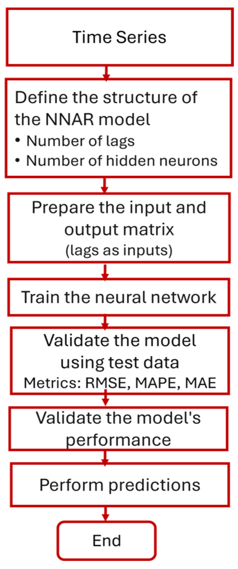
This process is summarized and visually presented in the following flowchart, which illustrates the architecture and data flow within the NNAR model (Figure 5).

2.2.4. Performance Indicators

In addition to producing forecasts, it is important to assess the predictive capacity of the proposed models [15,44], to ensure their accuracy and practical utility [45]. Traditionally, forecast performance evaluation is based on accuracy [46].
In this study, the following metrics were used to evaluate model accuracy: Mean Percentage Error (MPE), Root Mean Square Error (RMSE), and Mean Absolute Percentage Error (MAPE). Among the available metrics, MAPE is the most employed [47]. Generally, the most accurate model is selected as the one exhibiting the lowest error metrics, since its predictions provide estimates with minimal bias (small errors) and are close to actual values. These three metrics are defined as follows.
MPE calculates the error at each period as the ratio of the error in that period to the actual value of the corresponding period, followed by the average of these ratios.
M P E = 1 n i = 1 n ( y t y ^ t ) y t
RMSE is obtained as the square root of the mean squared error.
R M S E = 1 n i = 1 n ( y t y ^ t ) 2
MAPE measures the mean absolute percentage error, indicating how far the predicted values deviate from the actual data. It also reveals whether the chosen model tends to overestimate or underestimate the forecasts.
M A P E = 1 n i = 1 n ( y t y ^ t ) y t
To assess the statistical significance of differences in predictive performance among the evaluated models, the Diebold–Mariano (DM) test [48,49,50] was used. This test compares model accuracy and determines if observed differences are statistically significant based on forecast errors.

3. Results

The following Table 1 shows descriptive statistics of the monthly number of vessels transiting through the Panama Canal from January 2000 to December 2022.
The results (Table 1) show that the mean and median values are 1154 and 1145 vessels, respectively, with a standard deviation of 99 vessels. The maximum monthly maritime transit recorded in recent years is 1431 vessels, while the minimum is 890 vessels. Additionally, the first quartile (Q1 = 1082) and the third quartile (Q3 = 1216) represent the 25th and 75th percentiles, respectively, and provide information about the central dispersion of the data. These quartiles indicate that 50% of the monthly observations of vessels transiting the Panama Canal fall between 1082 and 1216 vessels.
The analysis of the historical data began with the decomposition of the original series to identify its behavior, including trend and seasonal patterns.
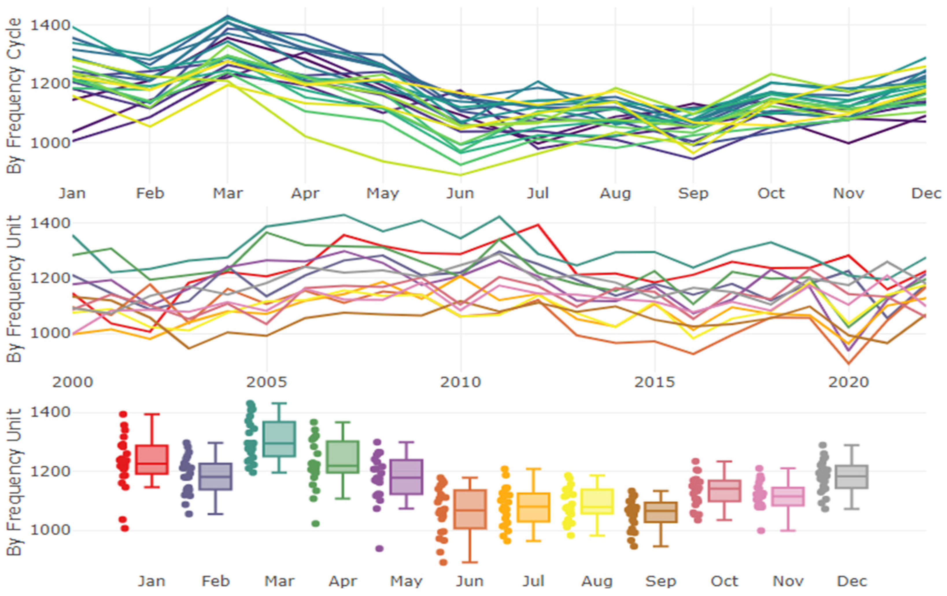
The number of vessels transiting the Panama Canal from January 2000 to December 2022 is relatively stable (Figure 6) and reveals a seasonal pattern with a recurrent 12-month cycle, as shown in Figure 7. The results indicate that maritime traffic through the Panama Canal is significantly higher from January to April compared to other months.
This set of visualizations provides a comprehensive view of fluctuations in frequency units, both monthly and annually, enabling a detailed analysis of the temporal dynamics of the series. The top panel displays the monthly evolution of the series across different calendar years (from January to December). Each line, distinguished by color, represents a full year and reveals recurring seasonal patterns as well as interannual variations in their magnitude and shape. The middle panel shows the temporal evolution disaggregated by month for the period from 2000 to 2022. In this case, each line and color correspond to a specific month, allowing for the analysis of behavior over time and facilitating the identification of month-specific trends and potential changes in seasonal patterns. Finally, the bottom panel presents boxplots summarizing the monthly distribution of the series values. This visualization clearly displays the median, interquartile range, dispersion, and presence of outliers, providing a concise and informative overview of the variability and relative stability of each month. In summary, the images presented in Figure 7 illustrate the behavior of irregularity by month and year. These results indicate that the series exhibits a strong component of high irregularity over time, with notable differences in the months of February and March, as well as in subsequent periods. From June onward, the series shows stability. Overall, the data do not display a pronounced trend (Figure 6).
The following sections present the visualization and temporal analysis of the data series, enabling the exploration of behavior over time and the identification of possible patterns.

3.1. Seasonal Autoregressive Integrated Moving Average Model (SARIMA Model)

The SARIMA model was employed due to the presence of a seasonal component in the series (see Figure 7). Initially, five model variants with significant parameters were identified based on the Akaike Information Criterion (AIC) and Schwarz Bayesian Criterion (BIC). Validation included checking the stationarity of the series and confirming the absence of autocorrelation in the residuals through autocorrelation plots and the Box–Ljung test. The autoregressive coefficients were then estimated to complete the model fitting. Subsequently, goodness-of-fit tests were conducted, evaluating the linearity and normality of the residuals to ensure the model met the diagnostic phase outlined by the Box–Jenkins methodology. Finally, the SARIMA (1,0,1)(0,1,1)12 model was selected for forecasting, demonstrating accurate short-term predictions and a significant seasonal influence on the number of vessels transiting the Panama Canal. The modeling process is presented below in a structured manner through diagrams that illustrate the key steps of the methodology.
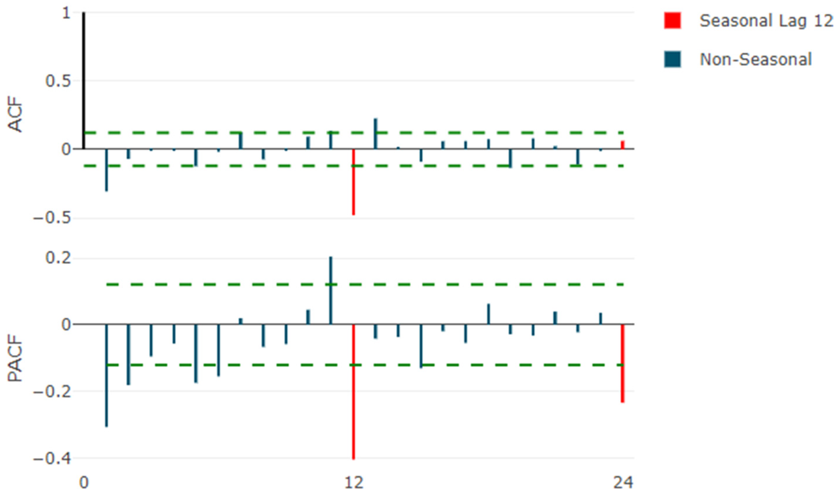
To verify the stationarity of the data, the Augmented Dickey–Fuller (ADF) test was applied. Upon identifying that the series was non-stationary, seasonal differencing was necessary to stabilize the mean and obtain a stationary series suitable for fitting the SARIMA model. This result was confirmed by the Dickey–Fuller test, which yielded an ADF statistic of −16.505 and a p-value of 0.01 (<0.05). Therefore, the development of the model was deemed appropriate. Subsequently, the autocorrelation and partial autocorrelation plots of the stationary series were constructed (Figure 8).
Based on the lags of the autocorrelation and partial autocorrelation functions (Figure 8), and after testing and analyzing several models, the SARIMA (1,0,1)(0,1,1) model was selected.
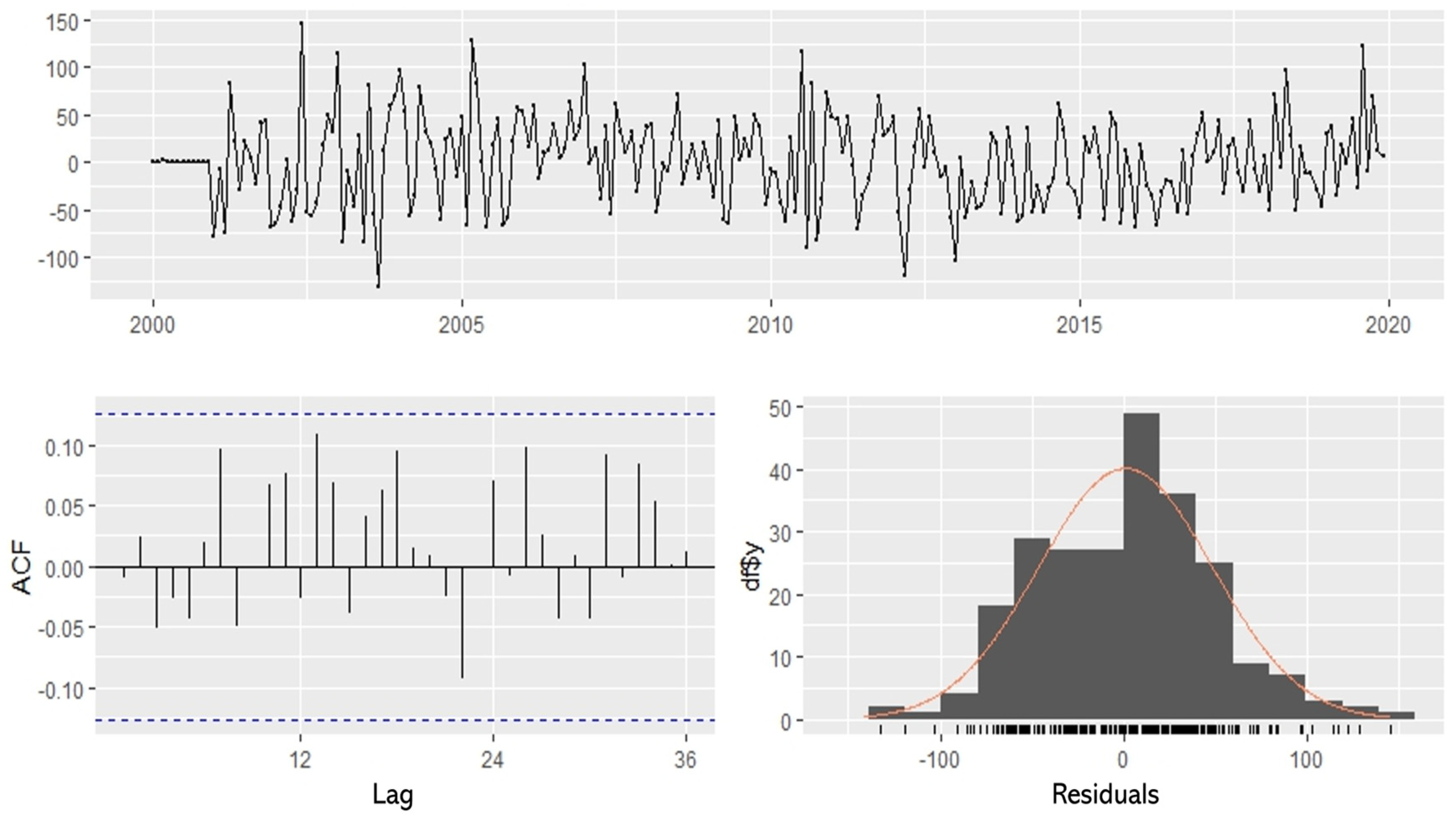
Figure 9 shows that the residuals (top panel) exhibit random behavior around zero, with no evidence of discernible patterns. The residual values (bottom left) lie within the confidence bands of the ACF plot, indicating no strong signs of autocorrelation. Additionally, in the residuals plot (bottom right), the values tend toward zero and approximate a normal distribution. These results confirm that the residuals behave like white noise, suggesting that the model satisfactorily captured the dynamics of the time series.

3.2. Holt–Winters Model

The time series of vessel transit exhibits seasonality; therefore, the Holt–Winters model was considered, and the corresponding plot of its behavior is presented below.
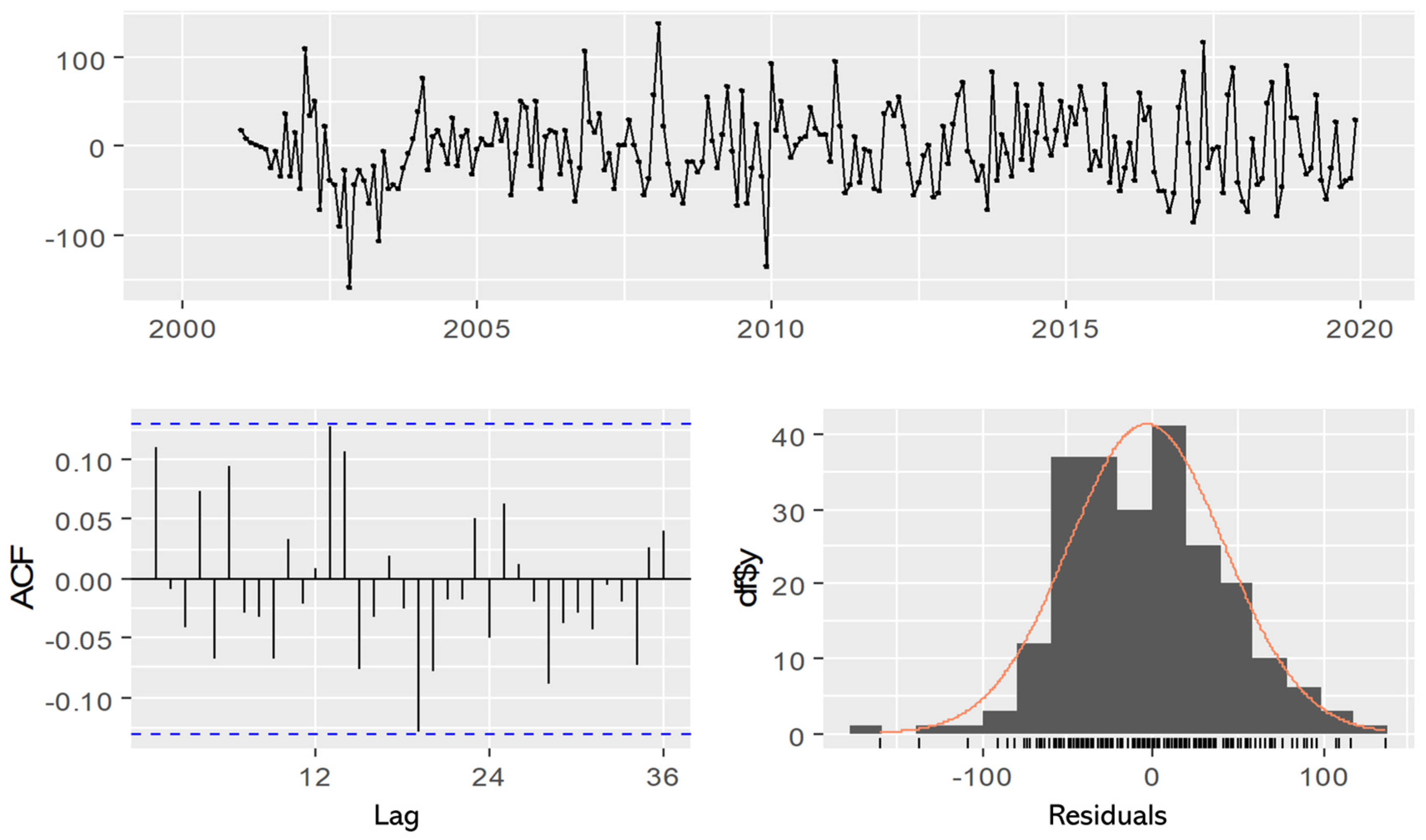
Figure 10 (top panel) does not display persistent or evident patterns, although some notable peaks may indicate outlier or extreme events, which are valid given the magnitude of the variable. The variability in the residuals is considered constant, although certain periods show greater dispersion, which may suggest some temporal instability.
In the residual autocorrelation function (bottom left), most of the bars fall within the significance bands (dotted blue lines), indicating no significant autocorrelation in the residuals. The histogram of the residuals with a superimposed normal curve (bottom right) suggests that the residuals behaved approximately normally. There are slight deviations in the tails, but not significant enough to invalidate the model.
Consequently, the Holt–Winters model adequately captures both the trend and seasonality of the data. This suggests that the selected Holt–Winters model is suitable for forecasting the analyzed time series.

3.3. Neural Network Model

Among the alternatives for modeling time series are neural network-based approaches, which have proven effective in capturing complex and nonlinear patterns in data. In this study, an NNAR (13,1,7)12 model was used, a variant of the autoregressive neural network specifically designed for time series. Based on this configuration, the model uses the last 13 lagged values of the series as input variables, performs first-order differencing to stabilize the series, and includes a hidden layer with seven neurons. The model was trained using the error backpropagation algorithm, which is based on the gradient descent method to optimize the neural network weights and minimize the objective error function. The seasonal component [12] maintains an annual periodicity, suitable for monthly frequency series. The logistic sigmoid function was used as the activation function; this choice was due to its traditional application in simple neural network architectures, widely used in time series analysis.
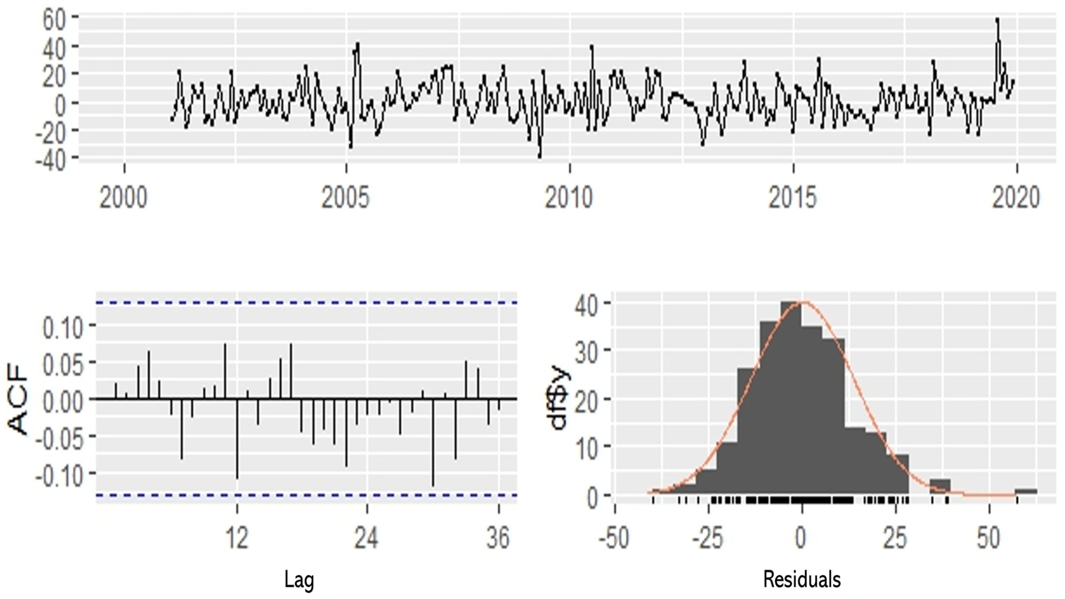
The interpretation of Figure 11 is the following: in the top panel, the residuals fluctuate around zero without any systematic or visible pattern, indicating randomness. The ACF plot (bottom left) shows no significant autocorrelations at the lags, suggesting the absence of serial correlation. In the histogram (bottom right), the residuals are approximately normally distributed. Based on this, the NNAR (13,1,7)12 model adequately captures the structure of the series, and it can be concluded that the residuals exhibit behavior consistent with white noise.

3.4. Model Comparison and Statistical Validation

The model comparison criteria are presented in Table 2. The table summarizes the error metrics (RMSE, MAE, and MAPE) for each model, along with the Box–Ljung test statistic and its corresponding p-value.
The comparative results of the models, in terms of error, show that the NNAR model achieved the lowest root mean square error (RMSE = 83.96) and a mean absolute percentage error (MAPE = 6.33) comparable to that of the SARIMA model (MAPE = 6.31). In contrast, the Holt–Winters model recorded the highest error metrics (RMSE = 106.17; MAE = 82.36; MAPE = 7.71), indicating a lower predictive capability.
In this same line of analysis, two out of the three models passed the Box–Ljung test ( A R I M A ( 1,0 , 1 ) ( 0,1 , 1 ) 12 , χ 2 = 15.9 , p = 0.72 ) and (NNAR χ 2 = 17.5 , p = 0.83 ) , indicating that the residuals do not exhibit significant autocorrelation; therefore, these models provide a good fit to the historical series. Similarly, it was confirmed that the parameter estimates of the aforementioned models are statistically significant (p > 0.05), suggesting that the models adequately captured the temporal structure of the data. By contrast, the Holt–Winters model produced a significant p-value (p = 0.00), indicating the presence of autocorrelation in the residuals and, consequently, a poor model fit. Overall, the results indicate that the SARIMA and NNAR models offer better predictive performance and greater statistical adequacy compared to the Holt–Winters model.

3.5. Diebold–Mariano (DM) Test

The results obtained from the Diebold–Mariano test are presented below (Table 3), in order to assess significant differences in the forecasting accuracy of the various models.
Based on the results presented in Table 3, observations can be made as the following: the positive DM statistic and the low p-value (0.012 < 0.05) indicate a statistically significant difference in performance between the SARIMA and Holt–Winters models. The positive sign suggests that the SARIMA model outperforms the Holt–Winters model in terms of forecasting accuracy. When comparing Holt–Winters and NNAR, the difference was even more pronounced (p < 0.001), confirming a significant disparity in accuracy between the two models at the 5% significance level, with NNAR clearly performing better. In contrast, the comparison between NNAR and SARIMA yielded a DM value close to zero (–0.07) and a high p-value (0.9442), which exceeds the 5% significance level, indicating no statistically significant difference; therefore, both models exhibited comparable predictive performance.
The forecasted number of vessels and the 95% confidence intervals for each model over the next twelve months (year 2023) are presented in Table 4.
Maritime traffic through the Panama Canal remains steady during the forecast period of 2023, with January and March representing the months with the highest vessel transit compared to the rest of the year.
The time series plots of the forecasts generated by the SARIMA, Holt–Winters, and NNAR models (Table 4), together with the training and testing data of vessel transits through the Panama Canal, are shown in Figure 12, Figure 13 and Figure 14.
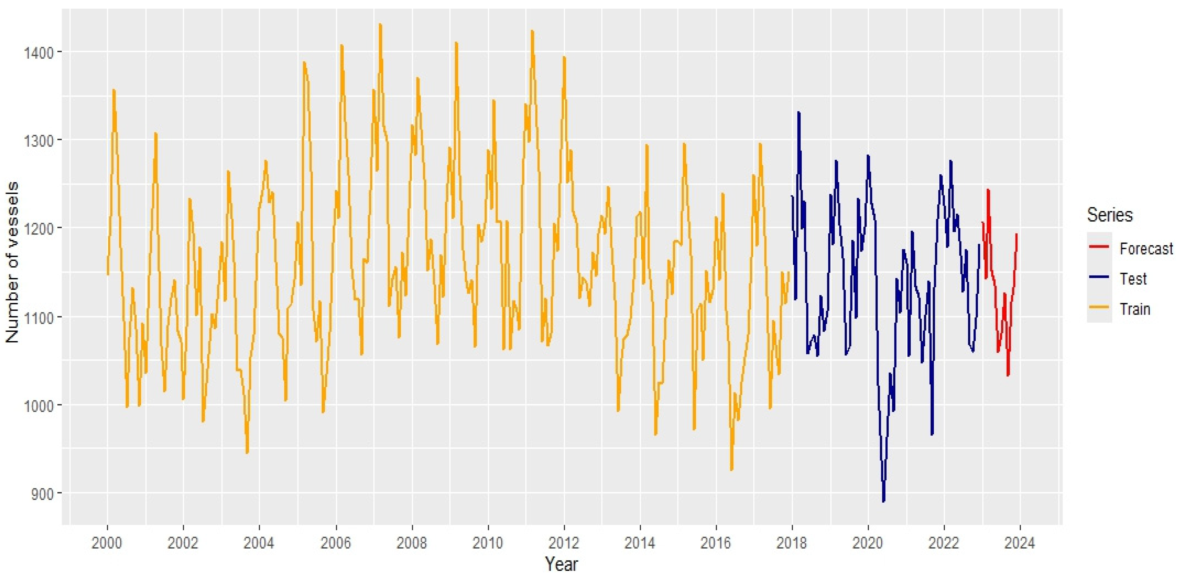
As shown in Figure 12, during the training period, represented in yellow, a consistent upward trend in maritime traffic was observed, accompanied by cyclical variations that suggest the presence of seasonality or recurring patterns in vessel flow. This evolution provides a robust foundation for modeling historical behavior. In the testing phase, marked in blue, the dynamic pattern is maintained, although with slight stabilization toward the later years. This behavior allowed for assessing the model’s generalization capability, indicating that it accurately replicates real conditions without signs of overfitting. Finally, the forecast segment, shown in red, projects a moderate continuation of the observed pattern. The model anticipates traffic levels similar to those previously recorded, reflecting an expectation of persistent behavior in the maritime system under similar conditions.
As shown in Figure 13, during the model training phase, highlighted in yellow, a sustained upward trend in the number of vessels is evident, accompanied by cyclical fluctuations that suggest a strong seasonal component in maritime traffic. In the testing phase, marked in blue, a gradual stabilization in vessel flow was observed. This stage allowed for validating the model’s ability to accurately replicate real conditions outside the training set, without loss of precision or signs of overfitting. Finally, the forecast segment, highlighted in red, projects a moderate continuation of maritime traffic levels. The model’s consistency with previous patterns suggests that similar operational conditions are expected in the future, reinforcing the model’s usefulness for short-term planning.
Figure 14 shows the time series of the number of vessels, segmented into training (yellow), testing (blue), and forecasting (red) phases. An initial increasing trend was observed, followed by stabilization and then a sustained projection, suggesting consistency in the dynamics of maritime traffic.
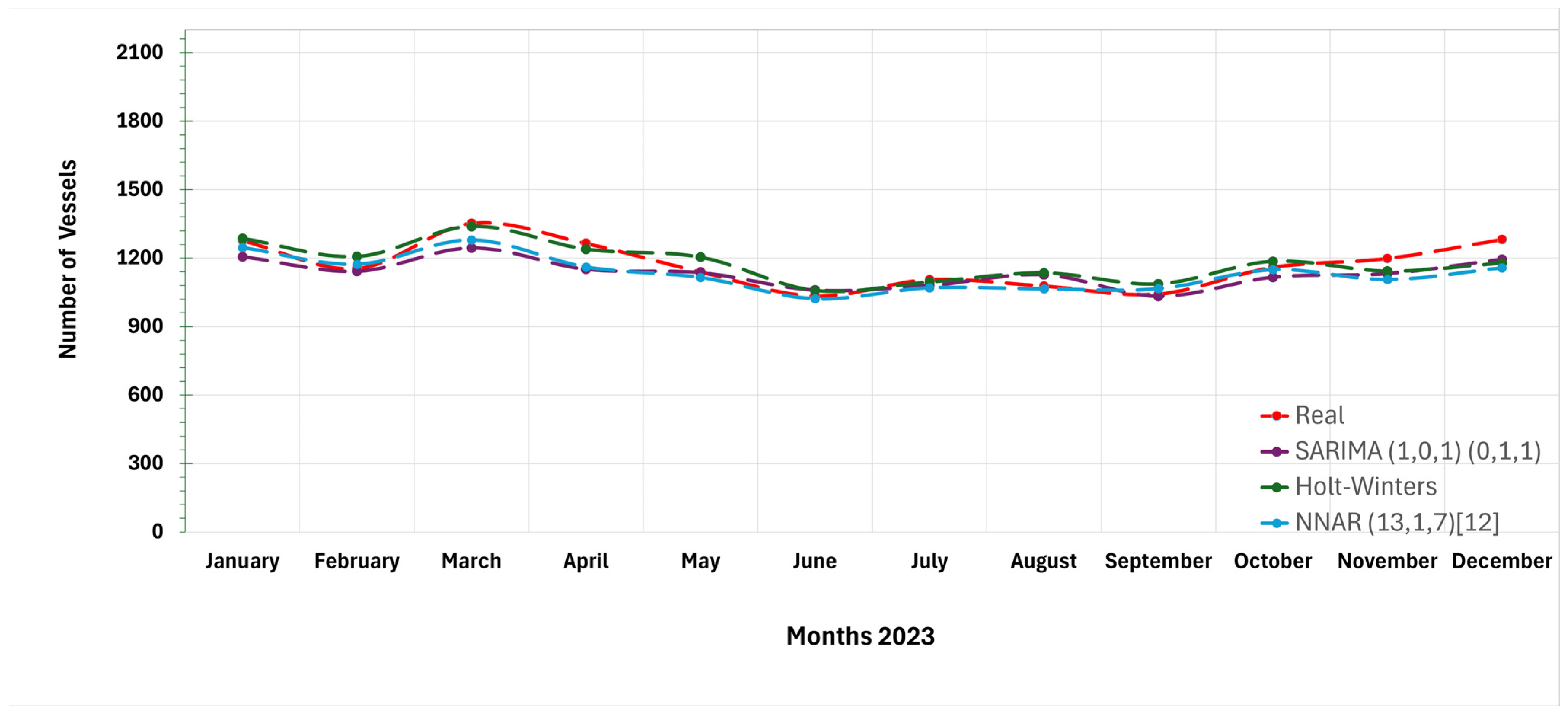
As a complement to the analysis conducted, a comparative representation is presented below between the empirical observations and the forecasts generated by the various evaluated models (Figure 15). This integrated visualization enabled a direct examination of discrepancies in the predictive performance of each model and facilitated the visual identification of the one that exhibited the greatest degree of fit to the historical series of vessel traffic through the Panama Canal.

4. Discussion and Conclusions

This study proposed forecasting methods based on both classical statistical models, such as ARIMA and Holt–Winters, and modern machine learning techniques using neural networks, with the objective of estimating the vessel traffic through the Panama Canal and comparing their performance. As noted by Wang et al. [51], reliable prediction of daily vessel traffic volume can support informed decision-making in operational management. Accordingly, various performance metrics were used to evaluate the robustness and accuracy of the forecasts [12,44].
In this study, three forecasting models were applied and compared as the following: the Seasonal Autoregressive Integrated Moving Average model (SARIMA), Holt–Winters exponential smoothing method, and Neural Network Autoregressive model (NNAR). The objective was to evaluate their performance in forecasting monthly vessel traffic through the Panama Canal, using standard evaluation metrics: Root Mean Squared Error (RMSE), Mean Absolute Error (MAE), and Mean Absolute Percentage Error (MAPE).
The results show that the NNAR model (RMSE = 83.96, MAE = 68.21, MAPE = 6.33%) and SARIMA model (RMSE = 87.58, MAE = 67.49, MAPE = 6.31%) achieved similar performance, whereas the Holt–Winters model exhibited considerably higher error values (RMSE = 106.17, MAE = 82.36, MAPE = 7.71%). Although SARIMA had slightly lower MAE and MAPE values, the NNAR model achieved the lowest RMSE, suggesting a better ability to capture the complexity of nonlinear patterns, as well as the seasonality present in the series. To determine whether these differences were statistically significant, the Diebold–Mariano test was applied. The results indicated statistically significant differences between the SARIMA and Holt–Winters models (DM = 2.61, p = 0.012), as well as between the Holt–Winters and NNAR models (DM = 5.31, p = 0.0001). In contrast, no significant differences were found between the NNAR and SARIMA models (DM = −0.07, p = 0.944), confirming that both offer comparable predictive accuracy.
These findings demonstrate that the neural network model achieved superior predictive performance compared to the SARIMA model in terms of error, thereby extending the empirical evidence reported by Gargari et al. [16] in predicting container ship traffic at Rajaee Port; by Ref. [52], who utilized neural networks to estimate marine traffic flow; and by Zhou et al. [53], who applied deep learning approaches for vessel flow forecasting. Additionally, a recent study combined an autoregressive time series model with a data assimilation method to predict the number of vessels transiting the Panama Canal, using data collected between 1 March and 31 March 2021 [26]. Although this analysis did not consider a long-term historical series, it represents the study most similar to ours identified in the literature.
Recent studies have employed machine learning techniques for forecasting in the maritime sector. Rao et al. [54] applied a variety of statistical, machine learning, and deep learning approaches for predictive analysis of port operations, with a specific focus on modeling vessel Total Stay Time and Delay Time. Similarly, Saber et al. [55] developed a hybrid machine learning-based approach for the accurate estimation of vessels’ estimated time of arrival at seaports. The combination of traditional statistical techniques with advanced deep learning approaches has led to significant advances in maritime traffic forecasting. These models provide valuable tools to support decision-making in port management and maritime transport planning.
The findings of this study on the temporal dynamics of vessel traffic through the Panama Canal are particularly relevant for the various stakeholders involved in maritime transport operations. Moreover, they represent a valuable tool for planning future investments in the port system, as the development of infrastructure expansion plans requires accurate and forward-looking forecasts of maritime traffic trends. Furthermore, these results could be generalized and applied to other maritime regions worldwide.
Future research may extend this work by comparing port traffic forecasts using alternative modeling approaches, such as GARCH models in cases where stochastic nonlinear behavior is detected, or other nonlinear methods such as Support Vector Machines, as well as enhancements to the neural network model applied in this study. Additionally, the inclusion of high-impact exogenous variables—such as extreme weather events (e.g., hurricanes, storms) and global climate patterns like El Niño and La Niña—could be considered, as these phenomena may significantly alter the dynamics of maritime transport. This complexity demands the use of robust predictive models capable of integrating multiple sources of variability to improve forecast accuracy.

Author Contributions

Conceptualization, M.C.-M.; methodology, W.E.; software, M.C.-M.; validation, A.R. and C.C.; formal analysis, C.C.; investigation, M.C.-M.; resources, M.C.-M.; data curation, W.E.; writing—original draft preparation, C.C.; writing—review and editing, A.R.; visualization, W.E. and A.R.; supervision, M.C.-M.; project administration, A.R. and C.C.; funding acquisition, M.C.-M. All authors have read and agreed to the published version of the manuscript.

Funding

This study was made possible thanks to the support of the Sistema Nacional de Investigación (SNI) of the Secretaría Nacional de Ciencia, Tecnología e Innovación (Panamá). Convocatoria Pública para el Ingreso de Nuevos Miembros al SIN de Panamá 2020 (Grant Number: SIN-NM2020). Contrato de Estímulo Económico del SIN No. 29-2021.

Institutional Review Board Statement

Not applicable.

Informed Consent Statement

Not applicable.

Data Availability Statement

Publicly accessible data were used, disclosed by Panamanian institutions such as the Panama Canal Commission, Panama Canal Authority, and National Institute of Statistics and Census of the Comptroller General of the Republic of Panama; additionally, data were obtained from the Presidente Roberto Chiari Library (Panama).

Conflicts of Interest

The authors declare no conflicts of interest.

References

  1. Bustamante Chong, M.; Bustamante Chong, C.; Caamaño Bustamante, V. Un Hub Logístico de Panamá y Su Impacto En Las Américas: Panama’s Logistics Hub and Its Impact on the Americas. J. Bus. Sci. 2020, 1, 23–36. [Google Scholar]
  2. Rodríguez Delgado, I. Estudio Inicial de Identificación de Invasiones de Peces Marinos En El Canal de Panamá: Un Enfoque de Metabarcoding. Master’s Thesis, Universidade da Coruña, Coruña, Spain, 2022. [Google Scholar]
  3. Sabonge, R. La Ampliación Del Canal de Panamá: Impulsor de Cambios En El Comercio Internacional. Available online: https://repositorio.cepal.org/entities/publication/50fbfaf5-228f-4abb-9541-e2eaf44a4551 (accessed on 1 February 2025).
  4. Huebner, G. Economic Aspects of the Panama Canal. Am. Econ. Rev. 1915, 5, 816. [Google Scholar]
  5. Carral, L.; Tarrío-Saavedra, J.; Naya, S.; Bogle, J.; Sabonge, R. Effect of Inaugurating the Third Set of Locks in the Panama Canal on Vessel Size, Manoeuvring and Lockage Time. J. Navig. 2017, 70, 1205–1223. [Google Scholar] [CrossRef]
  6. Carral, L.; Tarrio-Saavedra, J.; Castro-Santos, L.; Lamas-Galdo, I.; Sabonge, R. Effects of the Expanded Panama Canal on Vessel Size and Seaborne Transport. Promet-Traffic Transp. 2018, 30, 241–251. [Google Scholar] [CrossRef]
  7. Jakobsson, E.; Karlsson, L. The Consequences of Low Water Level in the Panama Canal and Possible Route Alternatives Comparing Four Routes Through and Around Panama from China to the US East Coast Regarding Emissions and Time Efficiency. Bachelor’s Thesis, Chalmers University of Technology, Gothenburg, Sweden, 2024. [Google Scholar]
  8. Canal de Panamá. Available online: https://pancanal.com/informes-anuales/ (accessed on 12 April 2025).
  9. Portal Logístico de Panamá. Available online: https://logistics.gatech.pa (accessed on 16 February 2025).
  10. Nie, Y.; Liu, K.; Xin, X.; Yu, Q. A Novel Through Capacity Model for One-Way Channel Based on Characteristics of the Vessel Traffic Flow. Int. J. Mar. Navig. Saf. Sea Transp. 2017, 11, 495–502. [Google Scholar] [CrossRef]
  11. Hasan, P.; Khan, T.D.; Alam, I.; Haque, M.E. Dengue in Tomorrow: Predictive Insights from ARIMA and SARIMA Models in Bangladesh: A Time Series Analysis. Health Sci. Rep. 2024, 7, e70276. [Google Scholar] [CrossRef]
  12. Serrano, A.L.M.; Rodrigues, G.A.P.; dos Martins, P.H.S.; Saiki, G.M.; Filho, G.P.R.; Gonçalves, V.P.; de Albuquerque, R.O. Statistical Comparison of Time Series Models for Forecasting Brazilian Monthly Energy Demand Using Economic, Industrial, and Climatic Exogenous Variables. Appl. Sci. 2024, 14, 5846. [Google Scholar] [CrossRef]
  13. Chudo, S.B.; Terdik, G. Modeling and Forecasting Time-Series Data with Multiple Seasonal Periods Using Periodograms. Econometrics 2025, 13, 14. [Google Scholar] [CrossRef]
  14. Sapundzhi, F.; Chikalov, A.; Georgiev, S.; Georgiev, I. Predictive Modeling of Photovoltaic Energy Yield Using an ARIMA Approach. Appl. Sci. 2024, 14, 11192. [Google Scholar] [CrossRef]
  15. Yadav, B.K.; Srivastava, S.K.; Arasu, P.T.; Singh, P. Time Series Modeling of Tuberculosis Cases in India from 2017 to 2022 Based on the SARIMA-NNAR Hybrid Model. Can. J. Infect. Dis. Med. Microbiol. 2023, 2023, 5934552. [Google Scholar] [CrossRef]
  16. Gargari, N.S.; Panahi, R.; Akbari, H.; Ng, A.K.Y. Long-Term Traffic Forecast Using Neural Network and Seasonal Autoregressive Integrated Moving Average: Case of a Container Port. Transp. Res. Rec. 2022, 2676, 236–252. [Google Scholar] [CrossRef]
  17. Yoo, S.-R.; Park, Y.-S.; Jeong, J.-S.; Kim, C.-S.; Jeong, J.-Y. A Forecast Method of Marine Traffic Volume through Time Series Analysis. J. Korean Soc. Mar. Environ. Saf. Res. Pap. 2013, 19, 612–620. [Google Scholar] [CrossRef]
  18. Xiaolei, L.; Jinli, X.; Mingjun, L. Research on Ship Traffic Flow Forecast Based on SARIMA Model. J. Wuhan Univ. Technol. 2017, 2, 329–332. [Google Scholar]
  19. Boudghene Stambouli, A.; Guizani, L. Neural Network-Based Prediction of Amplification Factors for Nonlinear Soil Behaviour: Insights into Site Proxies. Appl. Sci. 2025, 15, 3618. [Google Scholar] [CrossRef]
  20. Yoo, S.-L.; Kim, J.-S.; Jeong, J.-S.; Jeong, J.-Y. A Prediction of Marine Traffic Volume using Artificial Neural Network and Time Series Analysis. J. Korean Soc. Mar. Environ. Saf. 2014, 20, 33–041. [Google Scholar] [CrossRef]
  21. Millán, P.; Pérez, L.; Hontañón, P.; de Sabando, I. Modelización y Predicción Del Tráfico Marítimo En Los Puertos Españoles. An. De ASEPUMA 2019, 27, 1–17. [Google Scholar]
  22. Li, Y.; Liu, R.W.; Liu, Z.; Liu, J. Similarity Grouping-Guided Neural Network Modeling for Maritime Time Series Prediction. IEEE Access 2019, 7, 72647–72659. [Google Scholar] [CrossRef]
  23. Mostafa, M.M. Forecasting the Suez Canal Traffic: A Neural Network Analysis. Marit. Policy Manag. 2004, 31, 139–156. [Google Scholar] [CrossRef]
  24. Daranda, A. A Neural Network Approach to Predict Marine Traffic. Trans. Balt. J. Mod. Comput 2016, 3, 483–495. [Google Scholar]
  25. Ma, J.; Zhou, Y.; Chang, Y.; Zhu, Z.; Liu, G.; Chen, Z. TG-PGAT: An AIS Data-Driven Dynamic Spatiotemporal Prediction Model for Ship Traffic Flow in the Port. J. Mar. Sci. Eng. 2024, 12, 1875. [Google Scholar] [CrossRef]
  26. Tимoшeнкoвa, Ю.C.; Kyжбaнoвa, E.A.; Пopшнeв, C.B. Oпыт Пpoгнoзиpoвaния Интeнcивнocти Mopcкoгo Tpaфикa Ha Ocнoвe Koмпьютepнoгo Aнaлизa Online-Mopcких Kapт Пaнaмcкoгo Kaнaлa. Int. J. Open Inf. Technol. 2025, 13, 9–14. [Google Scholar]
  27. Panama Canal Commission 10 Year Report, FY 1980 to FY 1989: A Decade of Progress in Canal Operations and Treaty Implementation; The Panama Canal Commission: Washington, DC, USA, 1989.
  28. Instituto Nacional de Estadística y Censo. Available online: https://www.inec.gob.pa/buscador/Default.aspx? (accessed on 13 April 2025).
  29. Mgale, Y.J.; Yan, Y.; Timothy, S. A Comparative Study of ARIMA and Holt-Winters Exponential Smoothing Models for Rice Price Forecasting in Tanzania. Open Access Libr. J. 2021, 8, 1–9. [Google Scholar] [CrossRef]
  30. R Core Team. A Language and Environment for Statistical Computing; R Foundation for Statistical Computing: Vienna, Austria, 2020. [Google Scholar]
  31. RStudio. Integrated Development for R; RStudio PBC: Boston, MA, USA, 2020. [Google Scholar]
  32. Aguirre, J. Introduccioón al Tratamiento de Series Temporales: Aplicacioón a Las Ciencias de La Salud; Dióaz de Santos: Madrid, Spain, 1994; ISBN 84-7978-153-X. [Google Scholar]
  33. Wang, J.; Du, Y.H.; Zhang, X.T. Theory and Application with Seasonal Time Series; Nankai University Press: Tianjin, China, 2008. [Google Scholar]
  34. Aladag, C.; Egrioglu, E.; Letters, C.K. Forecasting Nonlinear Time Series with a Hybrid Methodology. Appl. Math. Lett. 2009, 22, 1467–1470. [Google Scholar] [CrossRef]
  35. Jenkins, G. Time Series Analysis: Forecasting and Control; Holden Day: San Francisco, CA, USA, 1976. [Google Scholar]
  36. Makridakis, S.; Hibon, M. ARMA Models and the Box–Jenkins Methodology. J. Forecast. 1997, 16, 147–163. [Google Scholar] [CrossRef]
  37. Bakar, N.A.; Rosbi, S. Autoregressive Integrated Moving Average (ARIMA) Model for Forecasting Cryptocurrency Exchange Rate in High Volatility Environment: A New Insight of Bitcoin. Int. J. Adv. Eng. Res. Sci. 2017, 4, 130–137. [Google Scholar] [CrossRef]
  38. Hanke, J.; Wichern, D. Business Forecasting, 5th ed.; Pearson Education: London, UK, 1995. [Google Scholar]
  39. Winters, P.R. Forecasting Sales by Exponentially Weighted Moving Averages. Manag. Sci 1960, 6, 324–342. [Google Scholar] [CrossRef]
  40. Uriel, E.; Muñiz, M. Estadística Económica y Empresarial: Teoría y Ejercicios; Editorial AC: Madrid, Spain, 1993. [Google Scholar]
  41. Sudheer, G.; Suseelatha, A. Short Term Load Forecasting Using Wavelet Transform Combined with Holt–Winters and Weighted Nearest Neighbor Models. J. Electr. Power Energy Syst. 2015, 64, 340–346. [Google Scholar] [CrossRef]
  42. Negnevitsky, M. A Guide to Intelligence Systems; Pearson Education: London, UK, 2005. [Google Scholar]
  43. Elseidi, M. MSTL-NNAR: A New Hybrid Model of Machine Learning and Time Series Decomposition for Wind Speed Forecasting. Stoch. Environ. Res. Risk Assess. 2024, 38, 2613–2632. [Google Scholar] [CrossRef]
  44. Jierula, A.; Wang, S.; Oh, T.M.; Wang, P. Study on Accuracy Metrics for Evaluating the Predictions of Damage Locations in Deep Piles Using Artificial Neural Networks with Acoustic Emission Data. Appl. Sci. 2021, 11, 2314. [Google Scholar] [CrossRef]
  45. Hrehova, S.; Antosz, K.; Husár, J.; Vagaska, A. From Simulation to Validation in Ensuring Quality and Reliability in Model-Based Predictive Analysis. Appl. Sci. 2025, 15, 3107. [Google Scholar] [CrossRef]
  46. St-Aubin, P.; Agard, B. Precision and Reliability of Forecasts Performance Metrics. Forecasting 2022, 4, 882–903. [Google Scholar] [CrossRef]
  47. Hyndman, R.J.; Athanasopoulos, G. Forecasting: Principles and Practice. 2018. Available online: https://otexts.org/fpp2/ (accessed on 12 April 2025).
  48. Diebold, F.; Mariano, R.S. Comparing Predictive Accuracy. J. Bus. Econ. Stat. 2002, 20, 134–144. [Google Scholar] [CrossRef]
  49. Cappello, C.; Congedi, A.; De Iaco, S.; Mariella, L. Traditional Prediction Techniques and Machine Learning Approaches for Financial Time Series Analysis. Mathematics 2025, 13, 537. [Google Scholar] [CrossRef]
  50. Chen, H.; Wan, Q.; Wang, Y. Refined Diebold-Mariano Test Methods for the Evaluation of Wind Power Forecasting Models. Energies 2014, 7, 4185–4198. [Google Scholar] [CrossRef]
  51. Wang, S.; Wang, S.; Gao, S.; Yang, W. Daily Ship Traffic Volume Statistics and Prediction Based on Automatic Identification System Data. In Proceedings of the 2017 9th International Conference on Intelligent Human-Machine Systems and Cybernetics (IHMSC), Hangzhou, China, 26–27 August 2017; Volume 2, pp. 149–154. [Google Scholar]
  52. Wang, H.; Wang, Y. Vessel Traffic Flow Forecasting with the Combined Model Based on Support Vector Machine. In Proceedings of the 2015 International Conference on Transportation Information and Safety (ICTIS), Wuhan, China, 25–28 June 2015; Volume 3, pp. 695–698. [Google Scholar] [CrossRef]
  53. Zhou, X.; Liu, Z.; Wang, F.; Xie, Y. Using Deep Learning to Forecast Maritime Vessel Flows. Sensors 2020, 20, 1761. [Google Scholar] [CrossRef]
  54. Rao, A.R.; Wang, H.; Gupta, C. Predictive Analysis for Optimizing Port Operations. Appl. Sci. 2025, 15, 2877. [Google Scholar] [CrossRef]
  55. Saber, S.M.; Thowai, K.Z.; Rahman, M.A.; Hassan, M.M.; Thowai, Z.; Hassan, M.; Mainul Bari, A.B.M.; Raihan, A. High-Accuracy Prediction of Vessels’ Estimated Time of Arrival in Seaports: A Hybrid Machine Learning Approach Optimizing the Estimated Time of Arrival (ETA) For. Marit. Transp. Res. 2025, 8, 100133. [Google Scholar] [CrossRef]
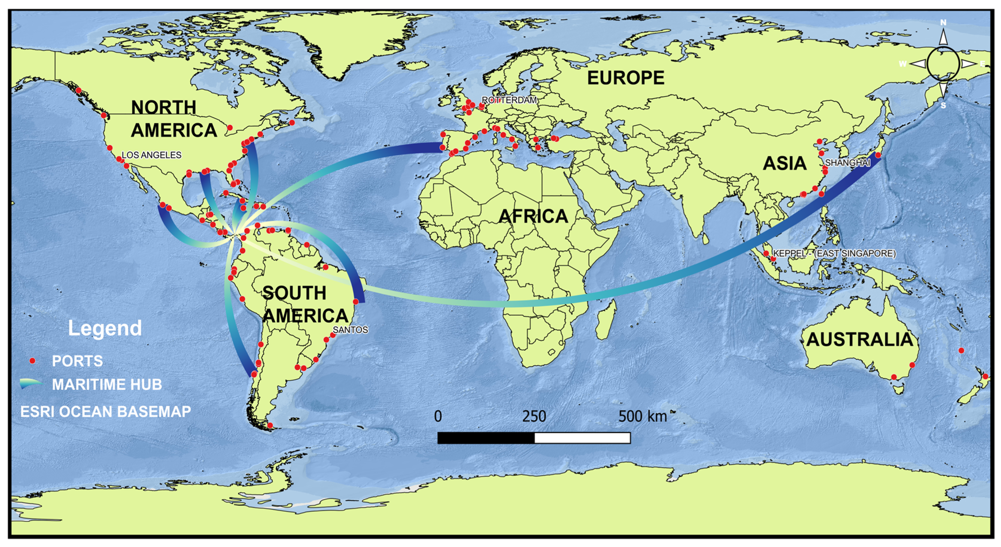
Figure 1. Vessel Transit Routes through the Panama Canal.
Applsci 15 08389 g001
Figure 2. ARIMA Modeling Process Flowchart.
Applsci 15 08389 g002
Figure 3. Holt–Winters Modeling Process Flowchart.
Applsci 15 08389 g003
Figure 4. Architecture of the Neural Network Model.
Applsci 15 08389 g004
Figure 5. Flowchart of the NNAR Model Architecture.
Applsci 15 08389 g005
Figure 6. Maritime transit through the Panama Canal, from 2000 to 2022.
Applsci 15 08389 g006
Figure 7. Decomposition of the time series into the trend, seasonal, and residual components.
Applsci 15 08389 g007
Figure 8. Autocorrelation Function (ACF) and Partial Autocorrelation Function (PACF).
Applsci 15 08389 g008
Figure 9. Forecast Using the SARIMA (1,0,1) (0,1,1) Model.
Applsci 15 08389 g009
Figure 10. Forecast Using the Holt–Winters Model.
Applsci 15 08389 g010
Figure 11. Forecast Using the NNAR (13,1 7)12 Model.
Applsci 15 08389 g011
Figure 12. Forecast Using the SARIMA   1,0 , 1   0 , 1 , 1 12 Model.
Applsci 15 08389 g012
Figure 13. Forecast Using the Holt–Winters Model.
Applsci 15 08389 g013
Figure 14. Forecast Using the NNAR (13,1,7)12 Model.
Applsci 15 08389 g014
Figure 15. Comparison between Actual Observations and Forecasts of Vessel Traffic through the Panama Canal Using the Evaluated Models.
Applsci 15 08389 g015
Table 1. Descriptive Statistics of Vessel Transit.
MeasureValues
Mean1154
Standard Deviation99
Minimum890
Maximum1431
First Quartile1082
Median1145
Third Quartile1216
Table 2. Model Effectiveness, Diagnostic Tests, and Fitting Results.
ModelEffectivenessBox–Ljung Test
RMSEMAEMAPE χ 2 p
SARIMA (1,0,1)(0,1,1) [12]87.5867.496.3115.900.72
Holt–Winters106.1782.367.7179.770.00
NNAR (13,1,7) [12]83.9668.216.3317.460.83
Table 3. The Diebold–Mariano Test.
ModelDM Testp-Value DMIs There a Significant Difference?
SARIMA and Holt–Winters2.61390.01204Yes
Holt–Winters and NNAR5.30640.000125Yes
NNAR and SARIMA−0.07160.9442No
Table 4. Comparison of Model Forecasts from January 2023 to December 2023.
Month/YearPrediction
S A R I M A   ( 1 , 0 , 1 )   ( 0 , 1 , 1 ) 12 H o l t W i n t e r s N N A R   ( 13 , 1 , 7 ) 12
Estimate95% CIEstimate95% CIEstimate95% CI
January 202312061105–130612861107–146512461201–1342
February 202311421028–125612071034–137911731134–1295
March 202312441124–136413391154–152512791215–1322
April 202311511028–127412391062–141611611073–1249
May 202311361011–126112041029–137911151025–1146
June 20231060935–11851058895–12211022972–1204
July 20231080955–12061095928–126510701016–1118
August 202311271002–12531135964–130710651013–1124
September 20231033907–11581087918–125510661016–1130
October 20231116990–124111861007–136511491082–1195
November 202311321006–12581143967–131811061075–1258
December 202311941068–13191178858–149811571120–1266
Disclaimer/Publisher’s Note: The statements, opinions and data contained in all publications are solely those of the individual author(s) and contributor(s) and not of MDPI and/or the editor(s). MDPI and/or the editor(s) disclaim responsibility for any injury to people or property resulting from any ideas, methods, instructions or products referred to in the content.