Emergency Resource Dispatch Scheme for Ice Disasters Based on Pre-Disaster Prediction and Dynamic Scheduling

Abstract

To address the challenge of dispatching emergency resources for community residents under extreme ice disaster, this paper proposes an emergency resource dispatch strategy based on pre-disaster prediction and dynamic scheduling. First, the fast Newman algorithm is employed to cluster communities, optimizing the preprocessing of resource scheduling and reducing scheduling costs. Subsequently, mobile energy storage vehicles and mobile water storage vehicles are introduced based on the ice disaster trajectory prediction to enhance the efficiency and accuracy of post-disaster resource supply. A grouped scheduling strategy is adopted to reduce cross-regional resource flow, and the dispatch routes of mobile energy storage and water vehicles are dynamically adjusted based on real-time traffic network conditions. Simulations on the IEEE-33 node system validate the feasibility and advantages of the proposed strategies. The results demonstrate that the grouped dispatch and scheduling strategies increase user satisfaction by 24.73%, average state of charge (SOC) by 30.23%, and water storage by 31.88% compared to global scheduling. These improvements significantly reduce the cost of community energy self-sustainability, enhance the satisfaction of community residents, and ensure system stability across various disaster scenarios.

1. Introduction

With global climate change, the frequency and intensity of extreme weather events has increased significantly. Ice disasters are a typical extreme weather phenomenon that represent one of the major hazards affecting the normal operation of cities and communities, Not only can paralysis of the power and water supply systems result in drastic deterioration of living conditions, it may also poses life-threatening risks under extreme circumstances [1,2]. Furthermore, ice disasters can cause long-term damage to infrastructure, worsen energy supply shortages, and lead to uneven water resource distribution [3,4]. Thus, how to efficiently dispatch emergency resources under ice disasters while ensuring the rapid restoration of normal supply post-disaster has become a critical issue in the emergency resource management.

Currently, traditional emergency resource dispatch strategies primarily rely on post-disaster response and static resource allocation information. Mobile energy storage vehicles and other necessary devices are allocated into different locations after the disaster occurs. However, because ice disasters often strike with sudden onset and prolonged impacts, traditional static resource scheduling methods exhibit significant limitations [5,6]. Studies have shown that the unpredictability and persistence of ice disasters render conventional static dispatch schemes inefficient in the recovery process, often failing to respond promptly to the urgent needs of affected areas [7]. Therefore, emergency management strategies based on pre-disaster prediction and dynamic scheduling have gained increasing attention. By leveraging pre-disaster information forecasting and resource preparedness, these strategies enable proactive resource allocation, thereby reducing the complexity of post-disaster scheduling and improving resource utilization efficiency [8]. Existing research primarily focuses on post-disaster resource allocation and recovery strategies, while the integration of pre-disaster predictive information to optimize resource dispatch under ice disaster conditions remains an area that has yet to be fully explored [9,10,11].

Existing studies have explored the introduction of dynamic scheduling methods [12,13] and path selection [14,15]. However, the application of these methods in ice disasters remains relatively limited, lacking both field verification and targeted strategies. Research has shown that mobile power sources, repair personnel, and network configurations can be coordinated to accelerate load restoration in power distribution systems [16,17,18,19]. Nevertheless, studies focusing specifically on mobile power dispatch are relatively scarce, and they rarely explore the feasibility and advantages of other mobile resources in enhancing the resilience of energy systems.

To address these issues, in this paper we propose an emergency resource dispatch strategy for ice disasters based on pre-disaster prediction and dynamic scheduling to improve resource allocation efficiency. Post-disaster scheduling costs are reduced by rationally grouping communities prior to the disaster and optimizing resource deployment and dispatch routes based on ice disaster trajectory predictions. Specifically, the fast Newman algorithm [20] is employed to cluster communities, thereby reducing the complexity of resource scheduling and optimizing resource allocation pathways. Furthermore, by integrating ice disaster trajectory predictions, we introduce both mobile energy storage vehicles and mobile water storage vehicles to enhance the efficiency and accuracy of post-disaster resource supply while ensuring stable energy and resource availability [21]. The implementation of this strategy not only significantly reduces the cost of community energy self-sustainability but also improves user satisfaction [22] while maintaining system stability under various disaster scenarios.

The main contributions of this paper are summarized as follows.

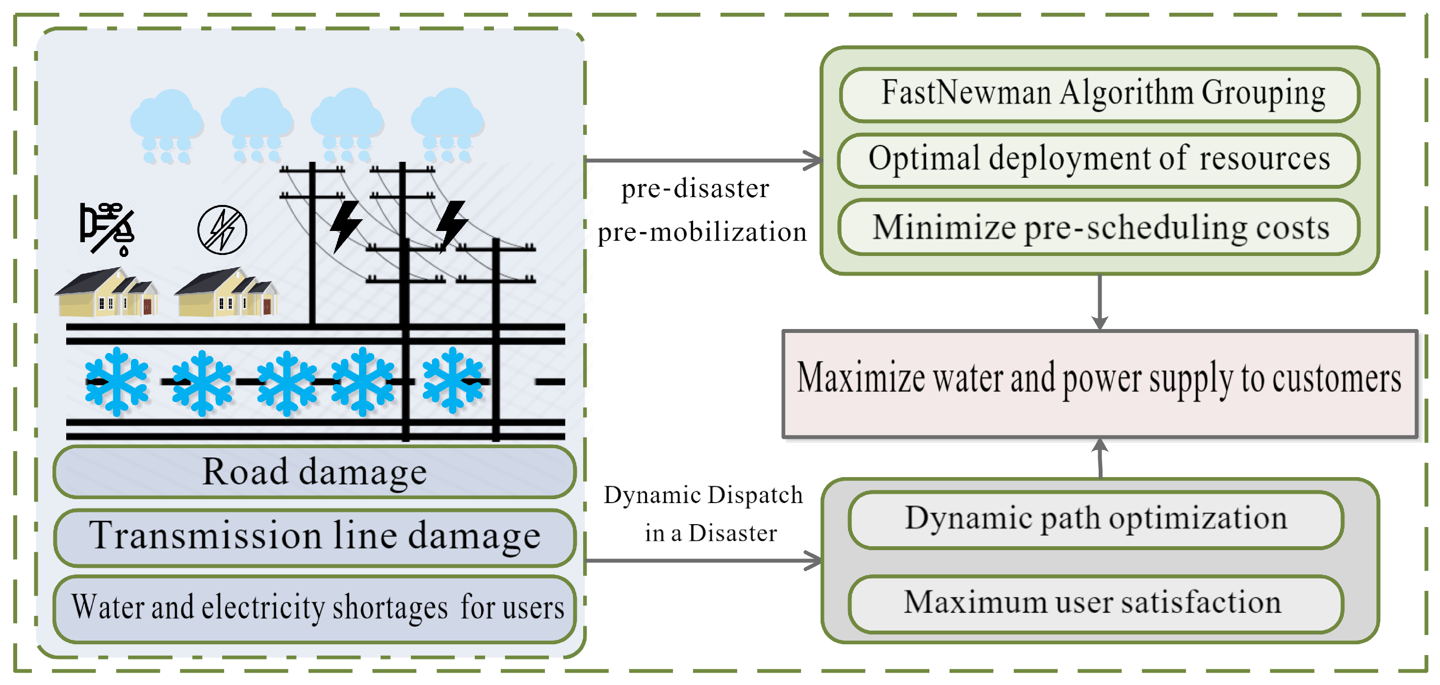
• Model Development: We propose a user satisfaction model based on response time, which comprehensively considers the timeliness of resource supply and scheduling efficiency.
• Optimization of Dispatch Scheme: By integrating ice disaster trajectory predictions, the fast Newman algorithm is employed for regional partitioning. In addition, mobile energy and water storage vehicles are pre-deployed before the disaster to improve emergency response speed.
• Resource Dispatch Optimization: A grouped scheduling strategy is adopted to reduce cross-regional resource flow and enhance resource utilization efficiency, while dispatch routes are dynamically adjusted based on real-time traffic network conditions to improve system stability and resilience.

The effectiveness of the proposed resilience-assessment method and enhancement strategy is validated through case studies of different scales. To facilitate a comprehensive understanding of the proposed approach, Figure 1 depicts the scheduling framework.

As illustrated in Figure 1, the scheduling framework highlights three key elements: the pre-disaster community grouping and resource pre-deployment process, the dynamic real-time dispatch stage, and the overarching objective of maximizing resource supply and user satisfaction. The remainder of this paper is organized as follows: Section 2 introduces the ice disaster scenario, develops the failure-rate model, and explains the community partitioning scheme based on the fast Newman algorithm; Section 3 formulates the integrated pre-disaster facility planning and spatiotemporal dispatch optimization; Section 4 presents comparative case studies on the IEEE-33-node system; finally, Section 5 concludes the paper, outlines current limitations, and discusses avenues for future research.

2. Failure Rate Modeling in Ice Disaster Scenarios

2.1. Ice Disaster Trajectory Prediction

To facilitate pre-disaster prevention and control planning, this study predicts the potential trajectory and impact areas of ice disasters based on data from the 2008 severe ice event in Hunan Province [23] and relevant meteorological data, as illustrated in Figure 2. In this figure, the green nodes denote community locations, the black nodes denote general system nodes, and the blue ellipses represent the predicted trajectory and affected regions of the ice disaster. This spatial prediction not only highlights the vulnerable areas within the network but also provides a critical basis for subsequent failure rate modeling and emergency-resource dispatch planning.

As an empirical model, it offers only a first-order approximation, and does not ingest real-time atmospheric updates or provide probability bounds. Future studies will refine this layer by coupling high-resolution numerical weather prediction output with machine learning ensembles so that forecast uncertainty can be quantified and incorporated into dispatch decisions.

2.2. Failure Rate Modeling

The highly dynamic spatial and temporal characteristics of ice disasters have profound impacts on power systems. Specifically, transmission line failures are mainly attributed to the combined effects of ice loads and wind loads. Ice loads exert vertical pressure due to ice and snow accumulation on conductors. To accurately assess failure rates, we employ differential equations to compute the rate of ice accretion based on the Kathleen F. Jones model [24,25] and establish an ice thickness model. In addition, the failure probabilities of both conductors and transmission towers are derived. The failure rate modeling consists of two main components: conductor failures and tower collapse. The specific calculation process is described below.

The failure rate of conductors is determined by considering the combined effects of wind and ice loads, as follows:

$$\begin{array}{c}\hfill P_{\mathrm{tension}}=\left\{\begin{array}{cc}0,\hfill & L_{\mathrm{total}}\le a_i\hfill \\ exp\left(\psi f\left({\displaystyle \frac{L_{\mathrm{total}}-a_i}{b_i-a_i}}\right)\right)-1,\hfill & a_i<L_{\mathrm{total}}<b_i\hfill \\ 1,\hfill & L_{\mathrm{total}}\ge b_i\hfill \end{array}\right.\end{array}$$

(1)

where $a_i$ and $b_i$ represent the lower and upper limits of the wind–ice gravity load, $L_{\mathrm{total}}$ is the combined load, and ${\psi }_f$ is the probability coefficient of line disconnection. The failure rate of the tower considers the total load borne by the tower, as follows:

$$\begin{array}{c}\hfill P_f=\left\{\begin{array}{cc}0,\hfill & T_{IW}\le a_W\hfill \\ exp\left({\psi }_w\left({\displaystyle \frac{T_{IW}-a_W}{b_W-a_W}}\right)\right)-1,\hfill & a_W<T_{IW}<b_W\hfill \\ 1,\hfill & T_{IW}\ge b_W\hfill \end{array}\right.\end{array}$$

(2)

where $a_W$ and $b_W$ represent the upper and lower limits of the total load, respectively, $T_{IW}$ is the total load, and ${\psi }_W$ is the collapse probability coefficient. Thus, the unified failure probability $P_{ij}$ of the line segment $ij$ is obtained as

$$\begin{array}{c}\hfill P_{ij}=1-\prod _{i=1}^z\left(1-P_{\mathrm{tension}}\right)\prod _{j=1}^z\left(1-P_f\right).\end{array}$$

(3)

2.3. Fast Newman Algorithm-Based Grouping Model

In disaster emergency resource dispatch, rational regional partitioning is crucial for improving resource allocation efficiency and reducing post-disaster dispatch costs. To achieve this, we adopt the fast Newman algorithm, a community detection algorithm based on Newman’s modularity optimization approach. It is an accelerated community aggregation algorithm proposed by Newman et al. [26], which builds upon the GN algorithm [27] to efficiently partition network structures. Compared with traditional community detection methods, the fast Newman algorithm offers significant computational efficiency advantages, making it well suited for complex and dynamic emergency resource dispatch tasks.

The fundamental principle of the fast Newman algorithm is to initially treat each network node as an independent community and then iteratively merge nodes. Each merging operation is determined by the principle of maximizing the modularity increment $\Delta Q$, prioritizing the combination of nodes that strengthen intra-community connections while minimizing inter-community links. The algorithm iterates by selecting merges that maximize the modularity increment until all nodes are merged into a single community or the modularity Q reaches its peak, after which it terminates and outputs the optimal community partitioning result. The detailed algorithmic steps can be found in [28].

Figure 3 illustrates the community partitions generated by the modified fast Newman algorithm, which divides the network into four distinct zones, each delineated with a different colored boundary (Zone 1 to Zone 4). These partitions correspond to groups of nodes with strong internal connectivity and limited external links, facilitating efficient and localized resource scheduling while minimizing cross-regional complexity and costs. The key steps of the modified fast Newman algorithm are summarized in Algorithm 1, which provides the computational basis for the network partitioning adopted in this study.

Algorithm 1 Modified fast Newman algorithm for finding max Q

Input: Network data, DERs allocation Output: Partitioned result   1: Calculate the entire PFS matrix;   2: Separate nodes into clusters and calculate $Q_0$;   3: while Number of clusters $\ne 1$ do   4:     if $\exists (c_i,c_j)=1$ then   5:         Group two clusters randomly;   6:     end if   7:     Calculate the increment of $\Delta Q$;   8:     Select the partitioning with maximum $\Delta Q$;   9:     Update Q according to the result of partitioning; 10:     Conserve the number of communities; 11: end while

3. Integrated Disaster Resource Scheduling Modeling

In extreme ice disaster environments, ensuring the stability of community energy supply presents significant challenges. Rational resource deployment prior to a disaster and efficient dynamic scheduling during the disaster are crucial for maintaining continuous power and water supplies. Therefore, we propose a multi-objective optimization model to optimize pre-disaster resource allocation and the deployment of charging stations and reservoirs as a way of improving post-disaster resource dispatch efficiency and system responsiveness.

3.1. Pre-Disaster Resource and Facility Optimization

During the pre-disaster defense planning phase, the core objectives of resource allocation optimization are to achieve efficient resource distribution, minimize dispatch costs, and enhance system stability and emergency response capability. Thus, the proposed objectives include the following targets:

• Minimization of Freshwater and Electricity Procurement Costs: By implementing rational community partitioning, resource demands in each region are optimally matched before the disaster to reduce procurement redundancy and waste while enhancing the accuracy of resource distribution.
• Minimization of Cross-Regional Resource Dispatch Costs: We apply the fast Newman algorithm for community partitioning to optimize scheduling efficiency within each region and reduce economic costs and transportation losses associated with inter-regional resource transfers while simultaneously enhancing the timeliness and accuracy of resource dispatch.
• Minimization of Deployment Costs for Mobile Energy Storage and Water Supply Vehicles: By optimizing regional partitioning, mobile energy storage vehicles and water supply vehicles can be strategically deployed to minimize dispatch distances, thereby improving resource allocation accuracy and reducing overall dispatch costs.
• Enhancement of Disaster Response Capability and System Reliability: Optimizing the layout of charging stations and reservoirs ensures efficient energy and water supplies during disasters while minimizing supply–demand gaps in high-priority load areas to improve system reliability and resilience [29].

To achieve the above four objectives, we propose a multi-objective optimization framework and formulate the corresponding objective functions: procurement costs, cross-regional dispatch costs, deployment costs of energy storage equipment and water supply vehicles, and pre-deployment of charging stations and reservoirs. The goal is to maximize pre-disaster resource allocation efficiency to ensure rapid post-disaster response.

3.1.1. Pre-Disaster Resource Optimization

Based on the optimization framework, we define the cost-minimization objective function as follows:

$$\begin{array}{c}\hfill \underset{x,d,r}{min}\left(c_w\left(x_w\right)+c_e\left(x_e\right)+c_d(d_w,d_e)+c_v(r_w,r_e)\right)\end{array}$$

(4)

where $x_w$ represents the total amount of freshwater resources, $c_w\left(x_w\right)$ is the total cost of purchasing freshwater resources, $x_e$ is the total amount of electricity resources, $c_e\left(x_e\right)$ represents the total cost of purchasing electricity resources $d_w$ and $d_e$ respectively denote the allocated amounts of freshwater and electricity resources, $c_d(d_w,d_e)$ denotes the allocation cost associated with the unit allocation price multiplied by the corresponding allocated quantity, $r_w$ and $r_e$ represent the number of deployed freshwater and energy storage vehicles, and $c_v(r_w,r_e)$ denotes the deployment cost, including fixed costs such as vehicle purchase, operation, and maintenance.

3.1.2. Pre-Deployment of Charging Stations and Reservoirs

In this section, an optimal pre-disaster deployment strategy for charging stations and reservoirs is proposed with the aim of enhancing the timeliness of post-disaster resource dispatch and improving overall system resilience. While regional partitioning plays a crucial role in optimizing resource allocation and ensuring resource balance within communities, the placement of charging stations and reservoirs should be further refined for effective emergency dispatch after a disaster. Specifically, charging station locations should be selected to minimize travel time from high-priority nodes to lower-priority nodes, ensuring that energy storage vehicles can supply power efficiently and promptly to critical load areas during a disaster. The corresponding objective function is

$$\begin{array}{c}\hfill min{G}_i=\sum _{i\in N}{b}_i\left(1-u_i^s\right){\gamma }_i{T}_i^D,\end{array}$$

(5)

where N denotes the set of all faulty load nodes. Here, $b_i\in \{0,1\}$, $u_i^s\in \{0,1\}$; if a charging station is deployed at load node i, then $b_i=1$, otherwise $b_i=0$. If a mobile energy storage vehicle can restore power supply to node i, then $u_i^s=1$; otherwise, $u_i^s=0$. In addition, ${\gamma }_i$ represents the weight coefficient of load node i, reflecting the importance of the node, while $T_i^D$ denotes the shortest travel time from charging station m to node i.

To ensure that mobile water supply vehicles can rapidly replenish water sources and prioritize restoring water supply to critical load nodes, the pre-disaster placement of reservoirs must also be strategically planned. The reservoir locations should be selected to minimize the total travel time from high-priority nodes to lower-priority ones. The corresponding objective function is

$$\begin{array}{c}\hfill min{G}_w=\sum _{i\in N}{b}_i\left(1-u_i^s\right){\gamma }_i{T}_i^{D,n},\end{array}$$

(6)

where $b_i\in \{0,1\}$, $u_i^s\in \{0,1\}$, $T_i^{D,n}$ denotes the shortest travel time from reservoir n to node i. These two models address the positioning problems of charging stations and reservoirs, respectively, in order to minimize the time cost of resource scheduling paths through optimal location selection while prioritizing the needs of high-weight nodes.

3.1.3. Constraints

To facilitate the effective dispatch of mobile energy storage vehicles and water supply vehicles across different regions under ice disaster while satisfying the electricity and water resource demands of all regions, the associated constraint conditions are as follows:

$$\begin{array}{cc}\hfill & \sum _{r=1}^R{x}_{r,a}\le X_{\mathrm{sum}},\sum _{r=1}^R{y}_{r,b}\le Y_{\mathrm{sum}}\forall r\in R,\hfill \end{array}$$

(7)

$$\begin{array}{cc}\hfill & D_{\mathrm{avail}}^r\le x_{r,a}{H}_a+y_{r,b}{F}_b\forall r\in R,\hfill \end{array}$$

(8)

$$\begin{array}{cc}\hfill & \sum _{r=1}^R{Q}_{\mathrm{elec},u,r}\le 1,\forall u\in U_e,\hfill \end{array}$$

(9)

$$\begin{array}{cc}\hfill & \sum _{r=1}^R{Q}_{\mathrm{water},w,r}\le 1,\forall w\in U_w,\hfill \end{array}$$

(10)

$$\begin{array}{cc}\hfill & \sum _{u\in U_e}{Q}_{\mathrm{elec},u,r}·W\ge D_{\mathrm{elec},r}\forall r\in R,\hfill \end{array}$$

(11)

$$\begin{array}{cc}\hfill & \sum _{w\in U_w}{Q}_{\mathrm{water},w,r}·W\ge D_{\mathrm{water},r}\forall r\in R,\hfill \end{array}$$

(12)

$$\begin{array}{cc}\hfill & T_{\mathrm{travel},r}\le T_{\max }\forall r\in R,\hfill \end{array}$$

(13)

$$\begin{array}{cc}\hfill & \sum _{r=1}^R{p}_r{D}_{\mathrm{avail}}^r\ge p_{\min }\forall r\in R,\hfill \end{array}$$

(14)

$$\begin{array}{cc}\hfill & y_{r,b}·F_b\le C_{\mathrm{vehicle}}\forall r\in R,b\in U_b,\hfill \end{array}$$

(15)

$$\begin{array}{cc}\hfill & I_{\mathrm{access},r}=1\forall r\in R,\hfill \end{array}$$

(16)

$$\begin{array}{cc}\hfill & E_{\mathrm{remain},r}\le E_{\min }\forall r\in R,\hfill \end{array}$$

(17)

where Equation (7) represents the overall constraint on the number of resources, while $X_{\mathrm{sum}}$ and $Y_{\mathrm{sum}}$ are the total numbers of water and energy storage vehicles, respectively. Equation (8) describes the resource demands in each region that should be satisfied, where $H_a$ is the capacity of a single water storage vehicle and $F_b$ is the power supply capacity of a single energy storage vehicle. Equations (9) and (10) define the unique allocation and capacity constraints for vehicles in each time period, ensuring that each vehicle can provide only one type of resource service at any given time. Equations (11) and (12) describe the conditions for meeting the electricity and water demands in each region, where $D_r^{\mathrm{elec}\mathrm{shortage}}$ and $D_r^{\mathrm{water}\mathrm{shortage}}$ respectively denote the shortage of electricity and water resources in region r and W represents the fixed resource capacity that each vehicle can carry. Equation (13) establishes the constraints on transportation distance and time, ensuring that the travel time $T_{\mathrm{travel},r}$ does not exceed $T_{\max }$. Equation (14) represents the resource priority constraints, taking into account the prioritization of resource demand across different regions. Here, $p_r$ denotes the priority weight of region r and $D_{\mathrm{avail}}^r$ represents the allocated resource amount to meet regional demand, which must not be lower than $p_{\min }$. Equation (15) imposes vehicle capacity constraints, ensuring that the power supply capability $F_b$ of energy storage vehicles does not exceed $C_{\mathrm{vehicle}}$, which guarantees safety and rationality in resource dispatching. Equation (16) specifies the path accessibility constraint, requiring that the path accessibility $L_{\mathrm{access},r}$ for each target region r must be equal to 1, which ensures that all planned routes remain feasible under the impact of the ice disaster. Equation (17) defines the energy consumption constraint, which requires that the remaining energy $E_{\mathrm{remain},r}$ of each vehicle after completing its assigned task must not be lower than the minimum energy requirement $E_{\min }$.

Building upon the aforementioned model formulation and constraint conditions, the resource deployment and infrastructure siting problem is formulated as a mixed-integer linear programming (MILP) model. To balance computational efficiency and solution accuracy, the model is implemented in MATLAB using the YALMIP toolbox and solved with the Gurobi optimizer [30]. By appropriately setting the time limit and optimality gap, the proposed approach efficiently yields the optimal pre-disaster resource allocation and infrastructure layout informed by predictive information.

3.2. User Satisfaction-Oriented Dynamic Scheduling Model

3.2.1. Spatiotemporal Scheduling Scheme

In the integrated power grid and transportation network system, the scheduling of mobile energy storage devices is determined by both their charge/discharge states and transportation states, exhibiting strong spatiotemporal coupling characteristics. Under disaster scenarios, power grid failures and road blockages significantly hinder traditional static resource scheduling, making it difficult to respond effectively to sudden disruptions. To address this challenge, this paper proposes a spatiotemporal dynamic scheduling model that comprehensively considers the transportation time $T_{\mathrm{new},i,m,n}\left(t\right)$ between node m and node n, the real-time traffic conditions, and the installation and configuration time of the equipment $T_{\mathrm{place},i}$. By incorporating these factors, the model enables the optimization of route selection and dispatch strategies, ensuring efficient and timely delivery of resources to affected areas during disasters. This enhances the efficiency of transportation path selection and energy supply responsiveness, ensuring that resources are deployed rapidly and accurately to the disaster-stricken regions.

The results of the proposed spatiotemporal scheduling model are visualized in Figure 4, which demonstrates the optimal spatial deployment and coordinated routing of mobile water/energy storage vehicles, charging stations, and reservoirs throughout the community network under ice disaster conditions. Each community zone is equipped with strategically sited charging stations (black icons) and reservoirs (blue icons), while mobile resource vehicles (green icons) are flexibly dispatched across nodes based on real-time network conditions and demand. This dynamic zone-aware scheduling approach enables balanced and efficient distribution of electricity and water resources even in the presence of extensive transmission line damage, thereby greatly enhancing the self-sufficiency and resilience of community energy systems during disasters.

To achieve this, our study incorporates two different optimization strategies, described below.

Path Planning and Dynamic Dispatch Optimization: Because ice disasters may cause road closures or traffic restrictions, route selection for mobile energy storage devices must be dynamically adjusted in real time based on changing traffic conditions to ensure that vehicles can select the optimal path and quickly deliver resources to the target communities.

Multi-Energy Coordination and Priority-Based Supply: During disasters, different communities exhibit varying demands for electricity, thermal energy, and water resources; therefore, we introduce a multi-energy coordination strategy to ensure that critical nodes receive priority in resource dispatch. Special emphasis is placed on essential facilities such as hospitals and fire stations to ensure their operational continuity. This prioritization improves the overall fairness and effectiveness of resource allocation.

3.2.2. Path Optimization for Mobile Energy Storage and Water Vehicles

Because transportation networks are highly susceptible to disaster impacts [31], unexpected events during an ice disaster can cause significant variations in the actual travel time of mobile energy storage vehicles along the same road at different time intervals and environmental conditions. To ensure reliability, this study incorporates factors such as road congestion and snow accumulation into traffic condition assessments [32]. A traffic congestion parameter is introduced to model the spatial relationship between the actual speed of mobile energy storage vehicles and the equivalent travel time.

The driving speeds of mobile energy storage and water vehicles are affected under disaster conditions; therefore, it is necessary to estimate their speed based on the congestion level A of the transportation network under disaster scenarios and the actual traffic conditions. The relationship between the travel time $T_{\mathrm{new},m,n}$ and the equivalent travel distance $L_{m,n}\left(t\right)$ between node m and node n with the actual vehicle speed $v_{\mathrm{new}}\left(t\right)$ can be expressed as

$$\begin{array}{c}\hfill v_{\mathrm{new}}\left(t\right)=v_0{e}^{-1.7\alpha },\end{array}$$

(18)

where $v_0$ represents the ideal vehicle speed and $\alpha$ denotes the congestion level of the transportation network under disaster conditions, which is related to the severity of the disaster and traffic flow. In practical applications, $\alpha$ can be estimated by assessing the impact of the disaster. Under disaster scenarios, the actual travel distance is influenced not only by geographical distance but also by road condition deterioration. To account for this, we introduce the equivalent travel distance $L_{m,n}\left(t\right)$ to represent the travel distance under disaster conditions:

$$\begin{array}{c}\hfill L_{m,n}\left(t\right)=L_{m,n,0}\left(1+{\displaystyle \frac{1}{v_{\mathrm{new}}\left(t\right)}}\right)\end{array}$$

(19)

where $L_{m,n,0}$ represents the geographical distance between node m and node n under normal conditions. Considering the impact of the disaster on road conditions, the travel time can then be expressed as

$$\begin{array}{c}\hfill T_{\mathrm{new},i,m,n}\left(t\right)={\displaystyle \frac{L_{m,n}\left(t\right)}{v_{\mathrm{new}}\left(t\right)}}.\end{array}$$

(20)

For each possible route, the travel times of all possible paths are calculated and the optimal path is selected to minimize travel time, as follows:

$$\begin{array}{c}\hfill T_{\mathrm{travel},\min }=\underset{r\in R_i}{min}{T}_{\mathrm{travel},r}.\end{array}$$

(21)

Therefore, the transportation network between communities j and k can be simplified into a single optimal mobility route, as illustrated in Figure 5.

Specifically, Figure 5a depicts the original transportation network, where each mobile energy storage vehicle may traverse multiple potential paths connecting various community nodes and resource depots (charging stations/reservoirs). After path optimization, as shown in Figure 5b, redundant and suboptimal routes are eliminated, resulting in a streamlined network in which each vehicle follows the most efficient route between resource depots and community nodes. This approach not only reduces overall travel distance and time but also improves scheduling efficiency and system resilience during disaster response.

3.2.3. User Satisfaction Maximization Objective Function

Under extreme conditions, the user satisfaction model is primarily determined by the timeliness of electricity and freshwater supplies as well as the extent to which supply meets demand. To analyze the impact of response time on user satisfaction, this study proposes an upper-level comprehensive satisfaction model based on response time, formulated as follows:

$$\begin{array}{c}\hfill S_i=\left\{\begin{array}{cc}1-\alpha ·{\displaystyle \frac{T_s^{\mathrm{response}}}{T_{\max }}},\hfill & \mathrm{if}{T}_s^{\mathrm{response}}\le T_{\max }\hfill \\ 0,\hfill & \mathrm{if}{T}_s^{\mathrm{response}}>T_{\max }\hfill \end{array}\right.\end{array}$$

(22)

$$\begin{array}{c}\hfill T_s^{\mathrm{response}}=T_{\mathrm{travel},\min }+T_s^{\mathrm{setup}}\end{array}$$

(23)

where $T_s^{\mathrm{response}}$ represents the response time of community s, which refers to the duration from the moment a community experiences a water and power outage to when it receives resources, while $T_{\max }$ denotes the maximum allowable response time of the system; if this time is exceeded, user satisfaction drops to zero. In this study, $T_{max}$ is a preset value mainly governed by the expected economic loss of prolonged power and water outages and the daily electricity and freshwater demand of the affected population; $T_{s,c}^{\mathrm{travel}}$ represents the time required for vehicle c to travel from its current location to community s, while $T_s^{\mathrm{setup}}$ refers to the loading and unloading time required for resupply operations in community s. In addition, $S_i$ represents the user satisfaction level of community i, indicating the degree of satisfaction of community residents with the timeliness of service in disaster emergency response, while $\alpha$ is the adjustment coefficient.

To optimize overall community user satisfaction, this study defines a maximization function for comprehensive user satisfaction $S_{\mathrm{total}}$, achieved by minimizing the response time for each community, as follows:

$$\begin{array}{c}\hfill max{S}_{\mathrm{total}}={\displaystyle \frac{1}{n}}\sum _{i=1}^n{w}_i·S_i,\end{array}$$

(24)

where n is the number of communities and $w_i$ denotes the weight of community i.

3.2.4. Constraints

We impose the following constraints:

$$\begin{array}{cc}\hfill & T_c^{\mathrm{resp}}\le T_{\max }\forall c,\hfill \end{array}$$

(25)

$$\begin{array}{cc}\hfill & T_{c1}^{\mathrm{resp}}\le T_{c2}^{\mathrm{resp}},\mathrm{where}{P}_{c1}>P_{c2},\hfill \end{array}$$

(26)

$$\begin{array}{cc}\hfill & SO{C}_c^{\mathrm{new},\min }\le SO{C}_c^{\mathrm{new}}\left(t\right)\le SO{C}_c^{\mathrm{new},\max }\forall c,t,\hfill \end{array}$$

(27)

$$\begin{array}{cc}\hfill & SO{C}_c^{\mathrm{new}}(t+1)=SO{C}_c^{\mathrm{new}}\left(t\right)+P_{\mathrm{charge}}-P_{\mathrm{use}}\forall c,t,\hfill \end{array}$$

(28)

$$\begin{array}{cc}\hfill & R_{m,n}\left(t\right)\le A_{m,n}\left(t\right),\forall m,n,t,\hfill \end{array}$$

(29)

$$\begin{array}{cc}\hfill & R_c^{\min }\le R_c^{\mathrm{alloc}},\forall c,\hfill \end{array}$$

(30)

$$\begin{array}{cc}\hfill & V_{\mathrm{available}}\left(t\right)\ge V_{\mathrm{required}},\forall t,\hfill \end{array}$$

(31)

where Equation (25) ensures that the response time $T_c^{\mathrm{resp}}$ of each mobile energy storage vehicle c does not exceed the maximum allowable time, guaranteeing that resources can reach each node within the specified time to meet emergency needs; Equation (26) ensures that the response time of high-priority vehicles is less than or equal to that of low-priority ones ($P_{c1}>P_{c2}$); Equation (27) ensures that the battery state of each mobile energy storage vehicle c at time t remains between the minimum allowable value $SO{C}_c^{\mathrm{new},\min }$ and that the maximum allowable value $SO{C}_c^{\mathrm{new},\max }$; Equation (28) represents the battery state variation of energy storage vehicle c between time t and $t+1$, considering both charging power $P_{\mathrm{charge}}$ and consumption power $P_{\mathrm{use}}$; and Equation (29) determines whether the path from node m to node n is feasible at time t. When the path feasibility parameter $A_{m,n}\left(t\right)=1$, the path is accessible; otherwise, the path is inaccessible. This ensures that the selected route remains viable under disaster conditions. Equation (30) ensures that the resource amount $R_c^{\mathrm{alloc}}$ obtained by each energy storage vehicle c meets the minimum resource guarantee requirement $R_c^{\min }$. This prevents excessive resource concentration in a subset of vehicles during emergencies, ensuring that the basic needs of all task nodes are met. Finally, Equation (31) ensures that the number of available vehicles $V_{\mathrm{available}}\left(t\right)$ at time t is not less than the minimum number $V_{\mathrm{required}}$.

Constraints of Mobile Energy Storage Vehicles

When a mobile energy storage vehicle needs to move from node m to n, it must first select the optimal route under disaster conditions in order to minimize the travel time $T_{\mathrm{ME},m,n}$. Prior to reaching node n, the mobile energy storage vehicle maintains a valid connection status. The spatial state scheduling constraints are as follows:

$$\begin{array}{cc}\hfill & \sum _{c=1}^C{\zeta }_{t,c}^{\mathrm{new}}+{\zeta }_{t,c}^{\mathrm{new}}=1,\forall t,\hfill \end{array}$$

(32)

$$\begin{array}{cc}\hfill & \sum _{t=t_0}^{t_0+h-1}{\zeta }_{t,c}^{\mathrm{new}}\ge h\left({\zeta }_{t_0-1,c}^{\mathrm{new}}-{\zeta }_{t_0-1,c}^{\mathrm{new}}\right),\forall t,c,\hfill \end{array}$$

(33)

$$\begin{array}{cc}\hfill & \sum _{t=t_0+1}^{t_0+h+1}\left({\zeta }_{t,c}^{\mathrm{new}}+{\zeta }_{t,c}^{\mathrm{new}}\right)\le 1,\forall t,c,\hfill \end{array}$$

(34)

where Equation (32) ensures the uniqueness of its location of mobile energy storage vehicle c, Equation (33) stipulates that the transmission time must not be less than h to ensure that the switching process meets the minimum required time, and Equation (34) ensures that the vehicle does not appear at multiple nodes simultaneously during the transmission time, which prevents state overlap and scheduling conflicts.

During charge–discharge scheduling between nodes, mobile energy storage vehicles must adjust their output power based on their energy state to support the power supply system, for which the following constraints must be satisfied:

$$\begin{array}{cc}\hfill & 0\le u_t^{\mathrm{new}}\le p_t^{\max \mathrm{esc}},\forall t,c,\hfill \end{array}$$

(35)

$$\begin{array}{cc}\hfill & u_t^{\mathrm{new}}+s_t^{\mathrm{new}}=p_t^{\mathrm{new}},\forall t,c,\hfill \end{array}$$

(36)

$$\begin{array}{cc}\hfill & SO{C}_t^{\mathrm{new}}=SO{C}_{t-1}^{\mathrm{new}}+\sum _t\left({\displaystyle \frac{p_t^{\mathrm{esc}}-p_t^{\mathrm{des}}}{e_{\max \mathrm{esc}}}}\right),\forall t,c,\hfill \end{array}$$

(37)

$$\begin{array}{cc}\hfill & SO{C}_t^{\mathrm{new},\min }\le SO{C}_t^{\mathrm{new}}\le SO{C}_t^{\mathrm{new},\max },\forall t,c,\hfill \end{array}$$

(38)

$$\begin{array}{cc}\hfill & p_t^{\mathrm{new}}=p_0^{\mathrm{new}},\forall t,\hfill \end{array}$$

(39)

where Equation (35) limits the charge–discharge power of mobile energy storage vehicle c, ensuring that its charge–discharge power does not exceed the maximum power $p_{\mathrm{esc}}^{\max }$ at any given time; Equation (36) states that vehicle c can only perform either charging or discharging at any moment; Equation (37) describes the relationship between the SoC of vehicle c and its charge–discharge power, ensuring that the battery state at time T is reasonably adjusted based on the previous time step and the input–output power; Equation (38) ensures that the SoCs of mobile energy storage vehicles remain within the allowable limits; and Equation (39) defines the transmission energy consumption.

Constraints of Mobile Water Storage Vehicles

Compared to the charge–discharge process of mobile energy storage vehicles, the loading and unloading of water can be completed relatively quickly. Without loss of generality, it is assumed that the total time required for water loading and unloading is 1 h.

Figure 6 illustrates two typical scheduling modes for mobile water storage vehicles in a post-disaster emergency scenario. The horizontal axis represents discrete time steps $(t,t+1,t+2,\cdots ,t+h,t+h+1,t+h+2)$, with the rows labeled “Mode 1” and “Mode 2” corresponding to different routing strategies. In the diagram, rectangular blocks filled in gray represent the transiting state (vehicles traveling between nodes), while those filled in orange represent the parking state (vehicles stopping for water loading/unloading). Mode 1 depicts continuous transit followed by a single parking interval, whereas Mode 2 features segmented transit interspersed with multiple parking events. The flexible scheduling framework enables mobile water storage vehicles to meet diverse water supply demands under dynamic emergency conditions.

The complete mode of transportation (represented by the gray sections in Figure 6) reflects the long-duration operation of mobile water storage vehicles, primarily designed for rapid response to water resource demands in the target areas. In contrast, the segmented transportation and operation mode depicts scenarios where mobile water storage vehicles need to make multiple stops for water loading or unloading during transit. This mode enhances scheduling flexibility and improves the capability to meet multi-site water supply demands. To better characterize the scheduling process, the specific spatiotemporal transition constraints are as provided as follows:

$$\begin{array}{cc}\hfill & T_{m,n}\left(t\right)+T_c^{\mathrm{load}/\mathrm{unload}}\le T_{\max },\forall m,n,c,t,\hfill \end{array}$$

(40)

$$\begin{array}{cc}\hfill & T_c^{\mathrm{load}}\le T_c^{\mathrm{transit}}(t+1)\le T_c^{\mathrm{unload}}(t+2),\forall t,c,\hfill \end{array}$$

(41)

$$\begin{array}{cc}\hfill & \sum _m{p}_{i,t}^{\mathrm{priority}}·T_{i,t}^{\mathrm{priority}}\ge p_{j,t}^{\mathrm{priority}},\forall i,j,t,\mathrm{where}{p}_{i,t}^{\mathrm{priority}}>p_{j,t}^{\mathrm{priority}},\hfill \end{array}$$

(42)

$$\begin{array}{cc}\hfill & T_c^{\mathrm{load}/\mathrm{unload}}\le h,\forall t,c,\hfill \end{array}$$

(43)

$$\begin{array}{cc}\hfill & T_{m,n}\left(t\right)={\displaystyle \frac{D_{m,n}}{v_{ij}\left(t\right)}},\forall t,m,n,\hfill \end{array}$$

(44)

where Equation (40) limits the total operation time of the water storage vehicle c within a given time period t; Equation (41) ensures that task execution follows a logical sequence, guaranteeing that loading, transportation, and unloading are carried out in the correct order; Equation (42) enforces a scheduling strategy that prioritizes high-priority tasks, i.e., or a given set of tasks i and j within the same time period t, if task i has a higher priority than task j, then the system must execute task i first; Equation (43) limits the total duration of loading and unloading tasks to not exceed the threshold h; finally, Equation (44) ensures that the transportation time is dynamically adjusted based on the distance $D_{m,n}$ and road conditions along the selected path.

At the water storage stations, mobile water storage vehicles can transport water between reservoirs. The constraints are as follows:

$$\begin{array}{cc}\hfill & -{\zeta }_{t,c}^{\mathrm{ws}}{p}_{t,c}^{\mathrm{ws}}\le p_{t,c}^{\mathrm{ws}}\le {\zeta }_{t,c}^{\mathrm{ws}}{p}_{t,c}^{\mathrm{ws},\max },\forall t,c,\hfill \end{array}$$

(45)

$$\begin{array}{cc}\hfill & SO{C}_{t,c}^{\mathrm{ws}}=SO{C}_{t-1,c}^{\mathrm{ws}}+{\eta }^{\mathrm{ws}}{\displaystyle \frac{p_{t,c}^{\mathrm{ws}}}{E_{\max }^{\mathrm{ws}}}},\forall t,c,\hfill \end{array}$$

(46)

$$\begin{array}{cc}\hfill & SO{C}_{t,c}^{\mathrm{ws}}\le SO{C}_{t,c}^{\mathrm{ws}}\le SO{C}_{t,c}^{\mathrm{ws},\max },\forall t,c,\hfill \end{array}$$

(47)

$$\begin{array}{cc}\hfill & \sum _{m,n}{\zeta }_{t,c}^{\mathrm{ws}}\le 1,\forall t,c,\hfill \end{array}$$

(48)

where Equation (45) ensures that the water loading/unloading power is subject to physical limitations, Equation (46) ensure that the water resource volume adapts to actual demand, Equation (47) restricts the water capacity of the storage vehicle within its limits, and Equation (48) ensures that the storage vehicle can travel along only one route or stop at a specific community during each time period.

Following the establishment of the user satisfaction objective and associated constraints, this problem is similarly formulated as a mixed-integer linear programming (MILP) model. The model is constructed in MATLAB 2021b using the YALMIP toolbox and efficiently solved with Gurobi to address the complex spatiotemporal and resource constraints, obtaining the optimal dispatch strategy for maximizing community user satisfaction under an extreme ice disaster scenario.

4. Case Study Analysis

4.1. Simulation Setup

To quantitatively evaluate the effectiveness of the proposed scheduling strategies, a simulation model is established. As illustrated in Figure 7, the upper panel depicts the coordinated recovery and dispatching center of the power grid, highlighting core functions such as restoring electricity and water supply and coordinating traffic route scheduling through information exchange. The lower panel visualizes the IEEE-33 node system, indicating transmission line damage and community zone layouts. Two distinct resource scheduling schemes are compared: a grouped scheduling approach based on the fast Newman algorithm, which reduces cross-regional dispatch complexity, and a non-grouped (global) scheduling scheme that allocates resources on a system-wide basis. This comparative analysis enables a comprehensive assessment of the impact of regional division on disaster response effectiveness and system resilience.

Through experimental calculations, the following emergency resources of two cases are included in the system model.

Case 1: Four diesel generators; four small charging stations; four small reservoirs; the number of mobile energy storage vehicles in the four regions is 10, 4, 11, and 8, respectively; the number of mobile water storage vehicles in the four regions is 8, 3, 9, and 7, respectively; the deployment locations of the charging stations are nodes 3, 10, 22, and 28; and the deployment locations of the reservoirs are nodes 1, 5, 13, and 27. Case 2: Four diesel generators; one large charging station; one large reservoir; 24 mobile energy storage vehicles; 21 mobile water storage vehicles.

We set the power capacity of one large charging station to be approximately equivalent to that of four small charging stations and the water loading/unloading capacity of one large reservoir to be approximately equivalent to that of four small reservoirs. The charging station and reservoir are deployed at nodes 5 and node 7, respectively. For ease of scheduling, the initial positions of mobile energy storage vehicles and mobile water storage vehicles are set at the charging station and reservoir locations.

The main simulation parameters are shown in

Table 1. Simulationparameters (indicative exchange rate: USD 1 ≈ CNY 7.2).

Parameter	Value	Parameter	Value
$E_e^{\max }$	1 MWh	$E_w^{\max }$	5 tons
$SO{C}_e^{\max }$	1	$SO{C}_w^{\max }$	1
$SO{C}_e^{\min }$	0.3	$SO{C}_w^{\min }$	0
$C_e$	50 yuan/kwh	$C_w$	30 yuan/ton
$C_e^{\mathrm{car}}$	200 yuan	$C_w^{\mathrm{car}}$	200 yuan
$C_e^{\mathrm{stat}}$	1000 yuan	$C_w^{\mathrm{res}}$	1000 yuan
${\eta }_{\mathrm{cha}}$	0.95	${\eta }_w^{\mathrm{fill}}$	0.99
${\eta }_e^{\mathrm{dis}}$	0.90	${\eta }_w^{\mathrm{dra}}$	0.98
$T_e^{\mathrm{power}}$	0.3 MW	$T_w^{\mathrm{total}}$	1 h

.

In the table, $E_e^{\max }$ and $E_w^{\max }$ represent the maximum carrying capacities of mobile energy storage vehicles and mobile water storage vehicles, respectively; $SO{C}_e^{\max }$ and $SO{C}_e^{\min }$ denote the respective maximum and minimum energy capacities of mobile energy storage vehicles; $SO{C}_w^{\max }$ and $SO{C}_w^{\min }$ represent the respective maximum and minimum water capacities of mobile water storage vehicles; $C_e^{\mathrm{sd}}$ and $C_w^{\mathrm{sd}}$ indicate the cost of power generation by diesel generators and the cost of purchasing water resources from reservoirs, respectively; $C_e^{\mathrm{car}}$ and $C_w^{\mathrm{car}}$ denote the dispatching costs of a single mobile energy storage vehicle and a single mobile water storage vehicle, respectively; $C_e^{\mathrm{stat}}$ and $C_w^{\mathrm{res}}$ represent the respective costs of constructing a charging station and a reservoir; ${\eta }_e^{\mathrm{cha}}$ and ${\eta }_e^{\mathrm{dis}}$ respectively refer to the charging and discharging efficiency of mobile energy storage vehicles; ${\eta }_w^{\mathrm{fill}}$ and ${\eta }_w^{\mathrm{dra}}$ respectively denote the water loading/unloading efficiency of mobile water storage vehicles; and $T_e^{\mathrm{power}}$ and $T_w^{\mathrm{total}}$ represent the charging rate of mobile energy storage vehicles and the time required for water loading and unloading, respectively.

Throughout the simulation, each time step corresponds to one hour and the assessment horizon spans 48 h after the onset of the ice disaster. All mobile energy and water storage vehicles have a nominal speed of 60 km/h on clear roads; their actual speed is reduced according to the traffic-impedance factor ${\gamma }_{m,n}$ (see Equation (18)), which captures the effects of road icing and congestion. Community freshwater demand is obtained by evenly distributing the annual total reported in [33] across 365 days, thereby assuming a uniform seasonal distribution. Outage penalty costs are $6000\mathrm{CNY}/\mathrm{MWh}$ for electricity and $30\mathrm{CNY}/(\mathrm{t}·\mathrm{h})$ for water, consistent with the cost items in

Table 2. Cost comparison of different cases.

	Electric Load Loss (yuan)	Food Load Loss (yuan)	Freshwater Load Loss (yuan)	Mobile Multi-Energy Storage Cost (yuan)	Diesel Generation Cost (yuan)	Total Cost (yuan)
Case 1	141,300	25,980	12,000	1178	8000	220,458
Case 2	225,300	40,920	9000	1878	8000	321,098

. Diesel generators are assumed to have sufficient fuel during the 48-h window. Each water loading/unloading operation is completed within one time step (1 h), whereas the charging duration depends on the vehicle’s residual state of charge and the rated charging power $T_e^{\mathrm{power}}=0.3$ MW; in both cases, queuing delays at stations or reservoirs are neglected.

4.2. Analysis of Simulation Results

Figure 8 and Figure 9 illustrate the SOC variations of mobile energy storage and water storage vehicles under the two scheduling schemes. In Case 1, the grouped scheduling strategy based on the fast Newman algorithm ensures that the resource demands of each region are prioritized, thereby avoiding resource wastage and scheduling delays caused by cross-regional dispatching. Through efficient allocation of resources within each region, the SOC decline curve of energy storage vehicles in Case 1 is relatively smooth, demonstrating high resource utilization efficiency. In contrast, Case 2 adopts a global scheduling strategy that disregards resource balancing across regions. As a result, regions with high demand experience resource shortages during peak periods, while resources in low-demand regions remain underutilized, leading to a decline in overall resource scheduling efficiency. Regarding SOC variations, some energy storage vehicles in Case 2 deplete their energy rapidly within 24 h, whereas others remain underutilized, further diminishing the overall resource utilization efficiency. The average SOC was calculated over the entire simulation period for both scheduling strategies. As shown in the results, the grouped scheduling strategy achieves a 30.23% higher average SOC compared to global scheduling, confirming its effectiveness in improving overall resource utilization.

Figure 10 and Figure 11 illustrate the variations in water storage levels. In Case 1, the scheduling paths of water storage vehicles are flexibly adjusted in real time based on demand, ensuring a stable water supply. During idle periods, water storage vehicles can promptly return to reservoirs for replenishment, ensuring that the water supply needs of each region are met in a timely manner. As a result, Case 1 is more effective in responding to fluctuations in water demand during disasters. In Case 2, the absence of regional division leads to water shortages in certain areas during peak demand periods, reducing water supply efficiency during disasters. This indicates that regional division can effectively enhance the flexibility and precision of water resource scheduling, ensuring a stable water supply during disaster scenarios. The average water storage was calculated over the entire simulation period for both scheduling strategies. As indicated by the results, the grouped scheduling strategy achieves a 31.88% higher average water storage compared to global scheduling, further demonstrating its superiority in enhancing water resource allocation and ensuring supply stability during disaster scenarios.

Figure 12 and Figure 13 illustrate the variations in user satisfaction under the two scheduling schemes. In Case 1, user satisfaction is calculated based on the resource scheduling conditions of each region and weighted according to the population proportion of each region to derive the overall satisfaction level. The simulation results indicate that user satisfaction in Case 1 remains relatively stable, with minor fluctuations, staying at a consistently high level within 48 h. Grouped scheduling improves user satisfaction in certain regions, demonstrating that the grouped scheduling strategy can accurately match resource demands across different regions to effectively reduce community dissatisfaction caused by insufficient resource supplies.

In contrast, due to the absence of regional division and the adoption of a global scheduling approach in Case 2, resource allocation becomes unbalanced during certain periods. This issue becomes particularly evident after 24 h, where user satisfaction declines significantly and exhibits greater fluctuations. In certain regions, resource shortages lead to a noticeable deterioration in user experience, ultimately resulting in a lower user satisfaction level compared to the weighted average. This outcome further validates the advantages of grouped scheduling in enhancing user satisfaction, indicating that a well-structured regional division and resource allocation strategy can significantly improve user experience and optimize the balance of resource supplies in disaster emergency resource scheduling. The average user satisfaction was calculated over the entire simulation period for both scheduling strategies. The results show that the grouped scheduling strategy achieves 24.73% higher average user satisfaction compared to global scheduling.

The cost comparison of different cases is shown in Table 2. In the experiment, the penalty price for power load interruption is set at 6000 CNY/MWh. The interruption cost for freshwater load is set at 30 CNY/ton per hour, which is based on the transfer cost during the Daimon Island drought event [33]. Additionally, the total construction cost of charging stations and reservoirs for both Case 1 and Case 2 is assumed to be CNY 8000. All optimization models were solved using Gurobi.

As shown in Table 2, the total cost in Case 1 is significantly lower than that in Case 2, with an optimization margin of approximately 31.4%. This substantial cost reduction is primarily attributed to the adoption of the fast Newman algorithm for regional division, which optimizes resource scheduling. By segmenting regions, resource scheduling becomes more efficient, thereby avoiding additional costs and transportation losses associated with cross-regional resource transfers. Through precise resource deployment and a more efficient scheduling strategy, Case 1 ensures energy and water supply while minimizing unnecessary procurement and transportation expenses.

In contrast, Case 2 follows a global scheduling strategy without regional division. Although overall resource allocation is optimized, the lack of consideration of inter-regional resource balance leads to shortages in high-demand areas, subsequently increasing transportation costs and reducing resource utilization efficiency. This comparison demonstrates that the grouped scheduling strategy has significant economic advantages over the global scheduling strategy; it effectively enhances the timeliness and accuracy of resource scheduling, thereby significantly reducing overall costs.

4.3. Sensitivity Analysis

To further quantify the impact of key system parameters on user satisfaction, in this study we conducted sensitivity analyses of the maximum battery capacity limit (SOCmax) and maximum water storage limit (Water max). The corresponding simulation results are presented in Figure 14.

As shown in the figure, user satisfaction increases with the enhancement of either SOCmax or Water max; however, the rate of increase gradually slows as the parameters grow, exhibiting a clear trend of diminishing marginal returns. Specifically, when SOCmax and Water max are in the lower range, user satisfaction is highly sensitive to parameter changes; as the parameters approach their upper bounds, the satisfaction levels off and further increases have a limited effect.

In summary, it is recommended that in practical applications the upper limits of these parameters should be set reasonably by balancing system demand and economic considerations. This approach can enable optimal resource allocation and user satisfaction within the constraints of resource investment.

5. Conclusions

This paper proposes an emergency resource scheduling strategy for ice disasters by integrating the optimized deployment of mobile energy storage and water storage vehicles to enhance resource allocation efficiency and emergency response capability in disaster scenarios. Our simulation results show that the proposed grouped strategy increases user satisfaction by 24.73%, average state of charge (SOC) by 30.23%, and water storage by 31.88% in comparison to global scheduling while effectively reducing the self-sustaining cost of community energy and maintaining both high economic efficiency and system stability under extreme ice disaster scenarios. These findings further validate the advantages of the grouped scheduling strategy in optimizing resource allocation and enhancing system resilience, providing strong decision support for improving ice disaster emergency scheduling strategies. Future work will focus on integrating advanced disaster trajectory prediction models and conducting comprehensive sensitivity analyses on key system parameters to further enhance the robustness and adaptability of the proposed strategy.

References

1. Armenakis, C.; Nirupama, N. Urban impacts of ice storms: Toronto December 2013. Nat. Hazards 2014, 74, 1291–1298. [Google Scholar] [CrossRef]
2. Zhang, P.-F.; Tan, Y.-X.; Ai, J.-M.; Chen, R.; Gao, B.; Zhang, H.-X.; Jia, C.-J. Lessons learned from the ice storm in 2008 in Jiangxi China. In Proceedings of the 2009 Asia-Pacific Power and Energy Engineering Conference (APPEEC), Wuhan, China, 27–31 March 2009; pp. 1–4. [Google Scholar]
3. Duffey, R.B. Emergency systems and power outage restoration due to infrastructure damage from major floods and disasters. Insight 2020, 23, 43–55. [Google Scholar] [CrossRef]
4. Melaku, N.D.; Fares, A.; Awal, R. Exploring the impact of winter storm Uri on power outage, air quality, and water systems in Texas, USA. Sustainability 2023, 15, 4173. [Google Scholar] [CrossRef]
5. Li, L.; Tan, E.; Gao, P.; Jin, Y. Enhancing concurrent emergency response: Joint scheduling of emergency vehicles on freeways with tailored heuristic. Appl. Sci. 2024, 14, 7433. [Google Scholar] [CrossRef]
6. Mukhopadhyay, A.; Pettet, G.; Vazirizade, S.M.; Lu, D.; Jaimes, A.; Said, S.E.; Baroud, H.; Vorobeychik, Y.; Kochenderfer, M.; Dubey, A. A review of incident prediction, resource allocation, and dispatch models for emergency management. Accid. Anal. Prev. 2022, 165, 106501. [Google Scholar] [CrossRef]
7. Call, D.A. Changes in ice storm impacts over time: 1886–2000. Weather. Clim. Soc. 2010, 2, 23–35. [Google Scholar] [CrossRef]
8. Su, Z.; Zhang, G.; Liu, Y.; Yue, F.; Jiang, J. Multiple emergency resource allocation for concurrent incidents in natural disasters. Int. J. Disaster Risk Reduct. 2016, 17, 199–212. [Google Scholar] [CrossRef]
9. Yao, S.; Wang, P.; Liu, X.; Zhang, H.; Zhao, T. Rolling optimization of mobile energy storage fleets for resilient service restoration. IEEE Trans. Smart Grid 2019, 11, 1030–1043. [Google Scholar] [CrossRef]
10. Yao, S.; Wang, P.; Zhao, T. Transportable energy storage for more resilient distribution systems with multiple microgrids. IEEE Trans. Smart Grid 2018, 10, 3331–3341. [Google Scholar] [CrossRef]
11. Lin, Y.; He, C.; Zheng, L.; Ning, Y. Data driven urban power grid disaster prediction under extreme weather conditions. In Proceedings of the 2024 7th International Conference on Electronics Technology (ICET), Chengdu, China, 17–20 May 2024; pp. 1184–1190. [Google Scholar]
12. Ding, T.; Wang, Z.; Jia, W.; Chen, B.; Chen, C.; Shahidehpour, M. Multiperiod distribution system restoration with routing repair crews, mobile electric vehicles, and soft-open-point networked microgrids. IEEE Trans. Smart Grid 2020, 11, 4795–4808. [Google Scholar] [CrossRef]
13. Zhao, R.; Lu, J.; Chen, Y.; Gao, Y.; Li, M.; Wei, C.; Li, J. Active support strategies for power supply in extreme scenarios with synergies between idle and emergency resources in the city. Energies 2025, 18, 1940. [Google Scholar] [CrossRef]
14. Huang, K.; Jiang, Y.; Yuan, Y.; Zhao, L. Modeling multiple humanitarian objectives in emergency response to large-scale disasters. Transp. Res. Part E Logist. Transp. Rev. 2015, 75, 1–17. [Google Scholar] [CrossRef]
15. Huang, M.; Smilowitz, K.; Balcik, B. Models for relief routing: Equity, efficiency and efficacy. Transp. Res. Part E: Logist. Transp. Rev. 2012, 48, 2–18. [Google Scholar] [CrossRef]
16. Lei, S.; Chen, C.; Li, Y.; Hou, Y. Resilient disaster recovery logistics of distribution systems: Co-optimize service restoration with repair crew and mobile power source dispatch. IEEE Trans. Smart Grid 2019, 10, 6187–6202. [Google Scholar] [CrossRef]
17. Abdeltawab, H.H.; Mohamed, Y.A.-R.I. Mobile energy storage scheduling and operation in active distribution systems. IEEE Trans. Ind. Electron. 2017, 64, 6828–6840. [Google Scholar] [CrossRef]
18. Abdulrazzaq Oraibi, W.; Mohammadi-Ivatloo, B.; Hosseini, S.H.; Abapour, M. Multi-microgrid framework for resilience enhancement considering mobile energy storage systems and parking lots. Appl. Sci. 2023, 13, 1285. [Google Scholar] [CrossRef]
19. Chen, J.; Chen, C.; Duan, S. Cooperative optimization of electric vehicles and renewable energy resources in a regional multi-microgrid system. Appl. Sci. 2019, 9, 2267. [Google Scholar] [CrossRef]
20. Newman, M.E.J. Fast algorithm for detecting community structure in networks. Phys. Rev. E 2004, 69, 066133. [Google Scholar] [CrossRef]
21. Sui, Q.; Wei, F.; Wu, C.; Lin, X.; Li, Z. Self-sustaining of post-disaster pelagic island energy systems with mobile multi-energy storages. IEEE Trans. Smart Grid 2022, 14, 2645–2655. [Google Scholar] [CrossRef]
22. Yang, D.; Wu, Y.; Pandzic, H.; Tomin, N. Fault recovery of active distribution network considering translatable load and soft open point. J. Electr. Power Sci. Technol. 2024, 39, 183–192. [Google Scholar]
23. Zhou, B.; Gu, L.; Ding, Y.; Shao, L.; Wu, Z.; Yang, X.; Li, C.; Li, Z.; Wang, X.; Cao, Y.; et al. The great 2008 Chinese ice storm: Its socioeconomic–ecological impact and sustainability lessons learned. Bull. Am. Meteorol. Soc. 2011, 92, 47–60. [Google Scholar] [CrossRef]
24. Jones, K.F. A simple model for freezing rain ice loads. Atmos. Res. 1998, 46, 87–97. [Google Scholar] [CrossRef]
25. Yu, S.; Wei, C.; Fang, F.; Liu, M.; Chen, Y. Resilience assessment of electric-thermal energy networks considering cascading failure under ice disasters. Appl. Energy 2024, 369, 123533. [Google Scholar] [CrossRef]
26. Newman, M.E.J.; Girvan, M. Finding and evaluating community structure in networks. Phys. Rev. E 2004, 69, 026113. [Google Scholar] [CrossRef]
27. Girvan, M.; Newman, M.E.J. Community structure in social and biological networks. Proc. Natl. Acad. Sci. USA 2002, 99, 7821–7826. [Google Scholar] [CrossRef]
28. Wu, Q.; Su, X.E.; Jiang, L.; Huang, T.; Wang, X.; Sang, Y. Integrated network partitioning and DER allocation for planning of virtual microgrids. Electr. Power Syst. Res. 2023, 216, 109024. [Google Scholar] [CrossRef]
29. Borodinecs, A.; Zajecs, D.; Lebedeva, K.; Bogdanovics, R. Mobile off-grid energy generation unit for temporary energy supply. Appl. Sci. 2022, 12, 673. [Google Scholar] [CrossRef]
30. Gurobi Optimization, LLC. Gurobi Optimizer Reference Manual, Version 11.0. 2024. Available online: https://www.gurobi.com/documentation/ (accessed on 10 July 2025).
31. Xie, S.; Yang, Z.; Wang, M.; Xu, G.; Bai, S. Evaluating the resilience of mountainous sparse road networks in high-risk geological disaster areas: A case study in Tibet, China. Appl. Sci. 2025, 15, 2688. [Google Scholar] [CrossRef]
32. Lei, S.; Chen, C.; Zhou, H.; Hou, Y. Routing and scheduling of mobile power sources for distribution system resilience enhancement. IEEE Trans. Smart Grid 2018, 10, 5650–5662. [Google Scholar] [CrossRef]
33. Ren, C.; Dong, Y.; Xue, P.; Xu, W. Analysis of water supply and demand based on logistic model. IOP Conf. Ser. Earth Environ. Sci. 2019, 300, 022013. [Google Scholar] [CrossRef]
Figure 1. Ice disaster resource scheduling optimization.
Applsci 15 08352 g001
Figure 2. Community network based on ice disaster trajectory prediction.
Applsci 15 08352 g002
Figure 3. Ice disaster community network clustering based on fast Newman algorithm.
Applsci 15 08352 g003
Figure 4. Locations of mobile resource vehicles, charging stations, and reservoirs based on disaster scheduling.
Applsci 15 08352 g004
Figure 5. Path selection and optimization in resource scheduling.
Applsci 15 08352 g005
Figure 6. Mobile water storage routing based on classic scheduling.
Applsci 15 08352 g006
Figure 7. Transmission line damage and power grid coordination to restore dispatch.
Applsci 15 08352 g007
Figure 8. Comparative analysis of SOC variation between Case 1 (four regions) and Case 2 (one region).
Applsci 15 08352 g008
Figure 9. Comparative analysis of the average SOC of the four regions in Case 1 with the global SOC variation in Case 2.
Applsci 15 08352 g009
Figure 10. Comparative analysis of freshwater variation in of Case 1 (four regions) and Case 2 (one region).
Applsci 15 08352 g010
Figure 11. Comparative analysis of average freshwater in the four regions of Case 1 with the global freshwater scenario in Case 2.
Applsci 15 08352 g011
Figure 12. Comparative analysis of user satisfaction in Case 1 (four regions) and Case 2 (one region).
Applsci 15 08352 g012
Figure 13. Comparative analysis of average user satisfaction in the four regions of Case 1 with the global user satisfaction scenario in Case 2.
Applsci 15 08352 g013
Figure 14. Sensitivity analysis of user satisfaction with respect to SOCmax and Water max.
Applsci 15 08352 g014