1. Introduction
Binary classification (BC) is a very common machine learning (ML) task where each case is assigned to one of two possible outcome groups, called classes: the event class, e.g., “yes”, “disease”, and “high risk”, or non-event class, e.g., “no”, “no disease”, and “low risk” (
Table S1 provides a glossary of technical terms) [
1,
2,
3,
4,
5,
6,
7,
8,
9,
10,
11,
12,
13]. BC is widely used in various domains, such as fraud detection, spam filtering, finance, medical screening, clinical medicine, public health (PH), epidemiology, and social and technological sciences, where predictive models support risk prediction and stratification, early disease detection, targeted prevention strategies, and operational decision-making. Examples include identifying patients at high risk of hospital readmission, death, or other adverse outcomes; targeting preventive interventions toward high-risk subgroups; detecting fraudulent transactions or spam messages.
Performance of the predictive model depends critically on the appropriate selection of variables, making variable selection (VS) a key step in developing prediction models [
14]. It aims to identify a subset of variables that ensures high prediction accuracy and model simplicity, while avoiding overfitting, noise, and redundancy. This step can become particularly challenging in real-world tasks with high-dimensional datasets, collinearity between variables or weakly informative variables, and where class imbalances can additionally influence both model performance and evaluation. As imbalanced datasets are prevalent in real-world applications, VS is particularly important in these scenarios. Although various approaches have been proposed to address this issue, an imbalanced setting still poses a significant challenge in both model fitting and evaluation [
15,
16,
17,
18,
19,
20,
21,
22,
23,
24]. The predictive accuracy for the minority (usually event) class is typically of greater clinical or practical relevance, such as in rare diseases research, medical screening, and spam detection. Therefore, a model’s bias towards the majority (usually non-event) class can lead to serious consequences of false-negative results. In PH and clinical settings, where prediction tools inform resource allocation or treatment decisions, understanding prediction behaviors in both outcome classes is essential.
A common VS strategy is adding a candidate variable to an existing prediction model [
1,
25,
26]. Traditional evaluation metrics, such as the difference in the area under the receiver operating characteristic (ROC) curve (ΔAUC), the likelihood-ratio test (LRT), the difference in the Brier score (ΔBS), the Brier skill score (BSS), the net reclassification index (NRI), the difference in the F1-score (ΔF1-score), or the difference in a Matthews correlation coefficient (ΔMCC), are often used to assess the added predictive value of a candidate variable [
25,
26,
27,
28,
29,
30]. These methods provide global assessments of model performance and do not indicate whether a variable improves predictions for events, non-events, or both classes. Also, the visualization of results is often limited. These limitations become even more pronounced in imbalanced BC, where traditional methods often underperform and may fail to detect significant effects [
30,
31,
32,
33,
34,
35,
36,
37,
38,
39,
40]. This underscores the need for tools that not only evaluate model performance globally but also provide granular insights into class-specific behavior, especially when clinical outcomes depend on minority-class accuracy.
To address these limitations, we developed the U-smile method for evaluating the usefulness of a new variable in a BC model [
6,
7]. The U-smile method quantifies prediction changes with three families of interpretable coefficients and provides a standardized graphical summary in the form of the U-smile plot. This approach enables a detailed assessment of prediction improvement and worsening, separately in each outcome class. In two methodological studies, we validated and applied the U-smile method to both balanced and imbalanced BC settings and compared its results with established evaluation methods. Across tested scenarios, the U-smile method consistently outperformed traditional methods and proved highly effective in VS for BC.
This review outlines the U-smile method, summarizes main findings from its development and validation, presents its translational potential and future applications, and situates it within the broader context of explainable machine learning (XML) and explainable artificial intelligence (XAI).
2. Motivation Behind the U-Smile Method
Numerous methods and evaluation metrics have been developed for VS in BC. They differ in their underlying assumptions, sensitivity to subtle prediction changes, robustness to class imbalances, interpretability, and suitability for clinical applications.
Table S2 provides an overview of selected methods and metrics, summarizing their brief definitions, main strengths, and limitations, as well as relevance to imbalanced data contexts [
1,
3,
4,
6,
7,
12,
13,
14,
23,
25,
26,
28,
31,
33,
34,
36,
41,
42,
43,
44,
45].
Despite the breadth of available techniques, several limitations remain common across many approaches. Many traditional and ML-based methods yield a global assessment of variable importance and do not differentiate effects across outcome classes or operate as black box algorithms [
46]. As a result, they may fail to detect class-specific prediction improvements, particularly in imbalanced data scenarios, and their interpretability may be limited (
Table S2). The U-smile method overcomes these limitations by providing a class-stratified, transparent, and interpretable approach to variable selection.
A universal method for VS that would perform optimally in all settings does not exist. Every VS method and every ML algorithm has its inherent strengths and limitations that affect the final model performance. Therefore, model development and VS should be approached with methodological awareness to ensure that the chosen strategies are appropriate for the specific context and intended application [
14].
3. Overview of the U-Smile Method
The U-smile method [
6,
7] is a novel approach to evaluate whether a new variable added to a baseline model for binary classification improves its prediction separately for both outcome classes (
Figure 1). It was designed to address the limitations of traditional evaluation metrics, which often produce a single global measure of model performance and do not provide a separate assessment for both outcome classes, as well as lack an interpretable graphical summary of results. Additionally, the U-smile method combines a quantitative and visual evaluation of the usefulness of a new predictor. The U-smile method analyzes prediction errors and does not influence model training.
The U-smile method compares two nested models: a reference model, built using a baseline set of variables, and a new model that includes an additional candidate variable. For each individual, a prediction is made under both models, and the difference between the predicted probability and the true outcome, called the residual, is calculated. These residuals reflect prediction errors and form the basis for assessing whether the new variable led to better or worse predictions. An improved prediction is defined as a smaller prediction error (residual) under the new model compared to the reference model; a worsened prediction is defined as a larger prediction error.
The effect of the new variable at the individual level is visualized through a prediction improvement–worsening (PIW) plot with reference probabilities on the x-axis and new probabilities on the y-axis.
Then, through cross-tabulating the outcome class (non-event or event) with the direction of prediction change (better or worse), each individual falls into one of the four subclasses of the PIW matrix:
Non-events with improved prediction,
Non-events with worsened prediction,
Events with worsened prediction,
Events with improved prediction.
To quantify prediction changes, the U-smile method uses three families of coefficients:
BA coefficients express average absolute changes in prediction between new and reference models,
RB coefficients express relative changes in prediction between new and reference models relative to the prediction error of the reference model,
I coefficients express the proportions of individuals with prediction changes.
These coefficients are calculated at three levels of generality:
Level 1 (subclass-specific): Four values per coefficient family express prediction improvement and worsening in each subclass,
Level 2 (class-specific): Two values per coefficient family express net effects for non-events and events, calculated as the difference between improvement and worsening in each class,
Level 3 (overall weighted): One value per coefficient family expresses weighted averages of class-level net coefficients, accounting for class imbalance with weights proportional to class sizes.
For mathematical details and formulas of the BA-RB-I coefficients, please refer to our previous work.
The U-smile plot (
Figure 1, Step 3) provides a visual summary of the results. The four subclasses are shown in a fixed order on the x-axis, and the y-axis shows BA or RB coefficient values. The vertical distance between points in each class represents the values of class-specific net BA or RB coefficients. In the extended version of the U-smile plot, point sizes are scaled according to the corresponding I coefficient values, linking the magnitude of prediction changes with the proportion of affected individuals.
The shape of the U-smile plot (
Figure 2) provides an intuitive and immediate interpretation: a smile means prediction improvement, a frown—prediction worsening, a flatline—means no significant change in prediction, and a zigzag means prediction improvement in one class and worsening in the other.
4. Validation of the U-Smile Method
We proposed and validated the U-smile method in two methodological studies [
6,
7]. The first study established the method under a balanced scenario, while the second extended it to imbalanced scenarios and introduced additional enhancements. Together, these studies showed the U-smile method’s robustness and interpretability in a wide range of practical contexts.
4.1. Balanced Binary Classification
In the first study, we introduced the U-smile method as a novel method for evaluating the added predictive value of a candidate predictor [
6]. We built logistic regression models using real-world data from the Heart Disease dataset, available from the UCI Machine Learning Repository [
47,
48,
49], as well as synthetic data generated from theoretical probability distributions under informative and non-informative scenarios, as well as under dependent and independent scenarios.
A key finding was that the U-smile method consistently and reliably distinguished informative variables from non-informative ones. When informative variables were added to the reference model, the prediction improvement was reflected in double smile shapes of their U-smile plots. In contrast, non-informative variables generated flat or irregular shapes of their U-smile plots, indicating no meaningful improvement. Additionally, the U-smile method was robust to multicollinearity between variables included in the models. Compared to traditional evaluation metrics, such as the LRT and ΔAUC, the U-smile method provided more granular insights by assessing the effect of a new variable on prediction improvement and worsening separately for events and non-events. Moreover, the U-smile method did not produce any false-positive or false-negative results for synthetic data.
Also, we showed that the U-smile method’s numerical coefficients are closely related to established measures. Namely, using specific weights, ΔBS can be expressed in terms of the BA coefficients, the BSS in terms of the RB coefficients, and the I coefficient is derived from the NRI. The measures, combined with the graphical summary of the U-smile plot, enabled a comprehensive and intuitive evaluation of candidate variable usefulness under a balanced scenario.
4.2. Imbalanced Binary Classification
In the second study, we introduced and validated the three-level approach of the U-smile method for imbalanced binary classification [
7]. In addition to subclass-specific (Level 1) and class-specific net (Level 2) coefficients, a weighted overall level (Level 3) was defined. Level 3 aggregates net coefficients of Level 2 with weights proportional to class sizes, ensuring fair representation of both outcome classes in the overall assessment. Also, we scaled the point size in the U-smile plots of the BA and RB coefficients according to the I coefficient. This adjustment integrated the magnitude of prediction changes (BA and RB coefficients) and the number of prediction changes (I coefficient) in a single visual summary.
The U-smile method was tested on the same dataset as in the first study under seven predefined levels of class imbalance (1%, 10%, 30%, 50%, 70%, 90%, and 99% of the event class). Informative and non-informative variables, both real and generated, were evaluated at each imbalance level in logistic regression models.
Across the entire imbalance range, the U-smile method consistently distinguished informative variables from non-informative ones and remained robust and stable. Additionally, at high and extreme imbalance levels, the U-smile method detected both improvement in prediction in the minority class and reduction in overfitting to the majority class.
Compared to traditional metrics such as ΔAUC, ΔF1-score, ΔMCC, ΔBS, and BSS, the U-smile method was more sensitive to subtle but meaningful effects of informative predictors, especially at higher levels of class imbalance, where it outperformed these measures. Similar to the first study, the U-smile method did not produce any false-positive or false-negative results for generated data.
Table S3 shows a comparison of quantitative results of selected variable selection strategies for an informative variable (ST depression) and a non-informative variable (glucose) for models derived from the training dataset across imbalances ranging from 1% to 99% in the event class (adapted from Ref. [
7]).
5. Advantages of the U-Smile Method
The U-smile method has several methodological advantages over traditional approaches for evaluating variable usefulness in BC. They result from the U-smile method’s underlying design, i.e., combined residual-based assessment, stratification by outcome class, and joint numerical and graphical evaluations. These features work synergistically to provide a more granular, robust and interpretable evaluation framework that outperforms many traditional VS methods.
5.1. Stratified Assessment of Events and Non-Events
A separate assessment in each outcome class enables one to examine if a variable improves prediction selectively in one outcome class, which may indicate model bias or overfitting. This is particularly valuable in imbalanced data contexts and other applied tasks, such as PH and healthcare, where the clinical relevance may differ across outcome classes.
5.2. Robustness to Class Imbalance and Collinearity
U-smile method’s robustness to both class imbalance and collinearity between variables is particularly valuable in real-world applications where imbalanced datasets and correlations between variables are prevalent. VS methods providing global evaluation measures are often biased towards the majority class under imbalanced scenarios, and therefore may fail to detect improvements in the minority class. U-smile method’s weighted overall coefficients of Level 3 reflect class-size proportions of the dataset and enable a balanced global evaluation of a variable’s usefulness.
Table 1 summarizes U-smile method’s effectiveness across different levels of class imbalance and collinearity.
5.3. Visual Interpretability
The U-smile plot is a standardized graphical summary of prediction improvement and worsening in each outcome subclass. Its shape enables a swift and intuitive interpretation of results with smiles for prediction improvement, frowns for prediction worsening, flatlines for no changes, and zigzags for improvement in one class and worsening in the other. The U-smile plot’s design, where shape (smile/frown/flatlines/zigzags), color (class), and point size (proportion of individuals with changes in prognosis) encode key information, reduces the cognitive load for users, enabling faster and more accurate interpretations than tabular metrics. In applied contexts, such as model auditing, clinical decision-making, and PH policy decision-making, high visual interpretability of the U-smile plot supports more transparent and efficient communication with interdisciplinary audiences and non-technical stakeholders.
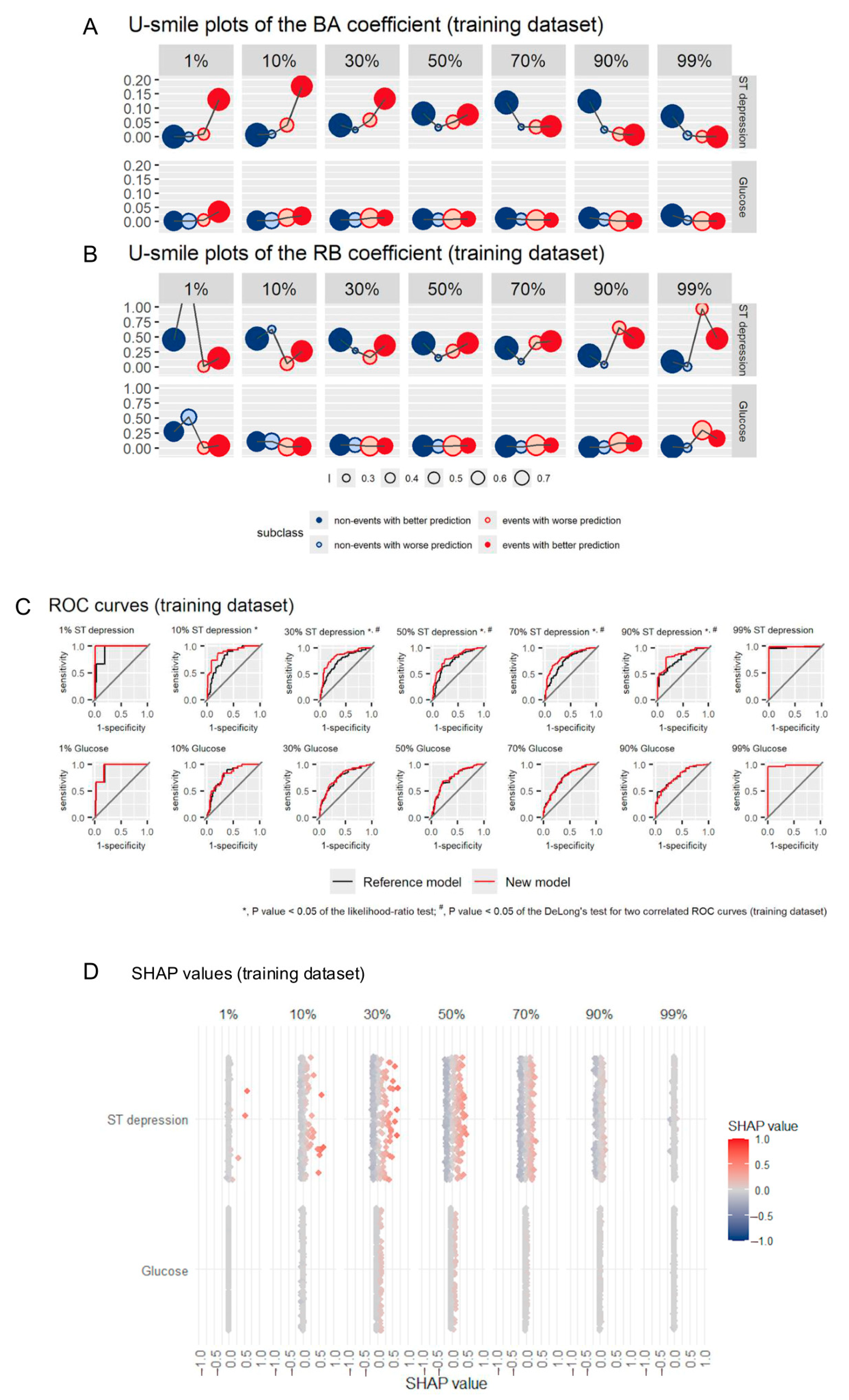
Figure 3 shows the U-smile plots of BA and RB coefficients (panels A and B, respectively), ROC curves (panel C) and SHAP values (panel D) for an informative (ST depression) and a non-informative (glucose) variable across imbalances ranging from 1% to 99% of the event class for the training dataset, presented side-by-side (adapted from ref. [
7]). The U-smile plots clearly reveal class-stratified prediction changes across the whole imbalance range, while ROC curves and SHAP values do not distinguish class-specific effects.
5.4. Sensitivity to Subtle Effects Through Stratified Evaluation
The residual-based BA and RB coefficients capture small but meaningful prediction changes separately in both subclasses. Such changes may not be reflected in global summary metrics. For example, a variable that improves predictions in the clinically important minority class may produce insignificant ΔAUC but will produce detectable BA and RB coefficient values, enabling a more nuanced and informed decision-making in VS (this was the case for 10% ST depression).
6. Limitations of the U-Smile Method
While the U-smile method offers significant advantages over traditional VS methods, several limitations remain and indicate directions for further methodological development toward more scalable and versatile applications.
Table 2 summarizes the main limitations of the U-smile method and corresponding areas for future research.
7. Future Translational Applications of the U-Smile Method
The U-smile method provides a comprehensive and interpretable approach for evaluating BC models, which makes it particularly valuable in contexts where transparency of model development and a separate evaluation for events and non-events are required.
7.1. Clinical Research and Public Health
The U-smile method can be directly applied to the development and evaluation of risk prediction models, screening tools, and biomarker assessments. A separate assessment for events and non-events can be particularly useful for planning and performing targeted PH interventions. Examples include tobacco control and identifying high-risk nicotine-product users for preventive measures, or stratifying patient populations to optimize financial and human resource allocation and reduce future healthcare costs. The U-smile method can also be used for electronic health records, digital health solutions, and PH surveillance systems, where predictive performance must be balanced with interpretability and implementation feasibility.
7.2. Integration with ML Pipelines
In applied ML workflows, the U-smile method can be a post hoc tool for evaluating variable usefulness and guiding model refinement. Embedded in decision-support systems or automated VS pipelines, it can provide complementary insights to techniques of explainable ML, such as SHapley Additive exPlanations (SHAP) or local interpretable model-agnostic explanations (LIME) [
50,
51,
52]. As it is conceptually compatible with any ML model that returns probability estimates, the U-smile method can be integrated in numerous algorithms, such as decision trees, random forests, or neural networks.
7.3. Real-Time Data
The availability of real-time health data, such as from wearable sensors, remote monitoring devices, or longitudinal tracking systems, is growing, and the U-smile method can be used to continuously update and recalibrate models. Potential applications include early detection of arrhythmias or atrial fibrillation from ECG data, analyzing fluctuations in sleep patterns, glucose levels, and body temperature. Another application can be in computer vision and autonomous vehicles, combined with parallel computation or dedicated hardware implementations [
53,
54,
55,
56]. In these settings, the U-smile method can support responsiveness and more informed decision-making.
7.4. Software Implementation
To increase the U-smile method’s accessibility and support its wider adoption among researchers and practitioners, an open-access software package and graphical user interface with interactive displays (e.g., R Shiny app) can be developed.
8. The U-Smile Method as XML and XAI Tool
Although the U-smile method was not designed to explain ML or AI predictions, but to evaluate the usefulness of a new variable in a model post hoc, it has the potential to contribute to the emerging fields of explainable machine learning (XML) and explainable artificial intelligence (XAI) [
10,
11,
52,
57]. The U-smile method is a VS method that evaluates how the prediction shifts due to a new variable, separately for both outcome classes. This feature is highly relevant in real-world tasks, including clinical, PH, and healthcare settings, where class imbalance is common, and explainability and interpretability of VS are critical.
The U-smile method provides both local and global evaluations of prediction changes due to an added variable in a model. By local evaluation, we refer to the assessments at the individual level through PIW matrices and PIW plots, and at the subclass level through the subclass-specific coefficients. Global evaluation is performed through the net coefficients at the class level and through the overall weighted coefficients at the model level. For more granular definitions, we can term the evaluation with the subclass-specific coefficients as semi-local evaluation (as it involves four subgroups of individuals, and the evaluation with the net coefficients as semi-global evaluation (as it involves whole classes).
The U-smile method produces intuitive and human-oriented visual output in the form of U-smile plots that support interpretability and communication across interdisciplinary settings. The U-smile plot can be swiftly and easily interpreted by various stakeholders thanks to its smiling, frowning, and flat plot shapes. This feature can help build trust in ML and AI systems, which is a key XAI goal.
By evaluating prediction changes in a class-stratified way, the U-smile method complements existing XML and XAI tools, such as SHAP and LIME, without overlapping their function [
50,
52]. SHAP and LIME explain model predictions, and the U-smile method explains the selection of model variables. SHAP values have been successfully used in the medical context for predicting acute kidney injury as well as procedure-related mortality and unplanned readmission [
58,
59]. Therefore, the U-smile method can contribute to transparency in model auditing and indicate potential bias in class-level performance. Also, Shapley values were proposed to be used to explain the ROC and precision–recall curves (PRC) as a measure of contribution of features toward the overall algorithm performance for feature selection tasks [
60]. Integrating Shapley values with the U-smile method remains an area for further methodological research.
9. Discussion
The U-smile method is a novel approach for graphical and quantitative evaluation of the added predictive value of candidate variables in binary classification tasks. It incorporates stratification by outcome class and a standardized graphical representation of results. Thus, it overcomes the main limitations of traditional evaluation methods, especially under class imbalance. The three-level structure of the U-smile method, comprising subclass-specific, class-level net, and overall weighted BA-RB-I coefficients, can be used for different analytic goals, and the U-smile plot offers a swift and intuitive visual summary to support interpretation of results.
In the two methodological studies, the U-smile method performed consistently and robustly in both balanced and imbalanced scenarios. As datasets with class imbalance are common in real-world applications, e.g., in rare diseases research reaching severe imbalance levels, a separate assessment of prediction improvement for events and non-events makes the U-smile method particularly effective in reducing bias towards the majority class during VS.
Conceptually, the U-smile method’s comprehensive and multi-level evaluation of a new variable in a model goes well beyond single global summary metrics: from individual PIW matrices and plots, through subclass- and class-specific coefficients, to global weighted coefficients. Although the method was not designed to explain why the model made a given prediction, it explains how predictions change with added variables in both classes. This aligns with the needs of XML and XAI to support transparent VS. The method’s alignment with FAIR principles (Findability, Accessibility, Interoperability, and Reusability) is another strength, as its outputs can be easily shared and compared across studies using the BA-RB-I coefficients and U-smile plots. Practically, the U-smile method is a user-oriented tool that ensures methodological transparency and translational potential to support informed decision-making in VS, especially in situations where understanding prediction behavior in both classes is critical.
10. Conclusions
Predictive modeling has become indispensable in clinical, precision, and personalized medicine, healthcare, PH, and other interdisciplinary fields that rely on informed decision-making. Therefore, explainable, transparent, and interpretable VS methods like the U-smile method are critical to making ML and AI more responsible, more ethical, and more trustworthy for patients, medical practitioners, and policy makers. Based on prediction changes comparison and class stratification, the U-smile method provides a framework for local and global VS evaluation, thus contributing to both XML and XAI. The U-smile method’s current shape already fills an important gap in the statistical and ML toolboxes, while the identified directions for future translational applications and methodological developments prove that the U-smile method is a growing framework.
Supplementary Materials
The following supporting information can be downloaded at
https://www.mdpi.com/article/10.3390/app15158303/s1, Table S1: Glossary of technical terms and their use in the U-smile method’s context; Table S2: Overview of selected methods and metrics for VS and model evaluation. Table S3: Comparison of quantitative results of selected variable selection strategies for an informative variable (ST depression) and a non-informative variable (glucose) for models derived from the training dataset across imbalance ranging from 1% to 99% of the event class. Shown are values of the class-specific BA-RB-I coefficients of Level 2, of the overall BA-RB-I coefficients of Level 3, as well as of selected global performance measures.
Author Contributions
Conceptualization, K.B.K., A.K., A.T.-F. and B.W.; methodology, K.B.K. and B.W.; software, K.B.K.; validation, K.B.K., A.K., A.T.-F. and B.W.; formal analysis, K.B.K. and B.W.; investigation, K.B.K., A.K., A.T.-F. and B.W.; resources, K.B.K., A.K., A.T.-F. and B.W.; data curation, K.B.K.; writing—original draft preparation, K.B.K.; writing—review and editing, K.B.K., A.K., A.T.-F. and B.W.; visualization, K.B.K. and B.W.; supervision, B.W.; project administration, K.B.K. and B.W.; funding acquisition, K.B.K., A.K. and A.T.-F. All authors have read and agreed to the published version of the manuscript.
Funding
This research received no external funding.
Institutional Review Board Statement
Ethical review and approval were waived for this study due to its nature as a review, which did not involve the collection or analysis of any human or animal data.
Informed Consent Statement
Not applicable.
Data Availability Statement
Conflicts of Interest
The authors declare no conflicts of interest.
Abbreviations
The following abbreviations are used in this manuscript:
| AI | artificial intelligence; |
| AUC | area under the curve; |
| BC | binary classification; |
| BS | Brier score; |
| BSS | Brier skill score; |
| LASSO | least absolute shrinkage and selection operator; |
| LIME | local interpretable model-agnostic explanations; |
| LRT | likelihood-ratio test; |
| MCC | Matthews correlation coefficient; |
| ML | machine learning; |
| NRI | net reclassification improvement; |
| PH | public health; |
| PIW | prediction improvement–worsening; |
| PRC | Precision–recall curve; |
| ROC | receiver operating characteristic; |
| SHAP | SHapley Additive exPlanations; |
| VS | variable selection; |
| XAI | explainable artificial intelligence; |
| XML | explainable machine learning. |
References
- Steyerberg, E.W. Clinical Prediction Models: A Practical Approach to Development, Validation, and Updating. In Statistics for Biology and Health, 2nd ed.; Springer: Cham, Switzerland, 2019; ISBN 978-3-030-16398-3. [Google Scholar]
- Flach, P. Machine Learning: The Art and Science of Algorithms That Make Sense of Data, 1st ed.; Cambridge University Press: Cambridge, UK, 2012; ISBN 978-1-107-09639-4. [Google Scholar]
- Clarke, B.; Clarke, J.L. Predictive Statistics: Analysis and Inference beyond Models. In Cambridge Series in Statistical and Probabilistic Mathematics; Cambridge University Press: Cambridge, UK, 2018; ISBN 978-1-107-02828-9. [Google Scholar]
- Brownlee, J. Imbalanced Classification with Python: Better Metrics, Balance Skewed Classes, Cost-Sensitive Learning; Machine Learning Mastery: Vermont, VIC, Australia, 2020. [Google Scholar]
- Kumari, R.; Srivastava, S.K. Machine Learning: A Review on Binary Classification. Int. J. Comput. Appl. 2017, 160, 11–15. [Google Scholar] [CrossRef]
- Kubiak, K.B.; Więckowska, B.; Jodłowska-Siewert, E.; Guzik, P. Visualising and Quantifying the Usefulness of New Predictors Stratified by Outcome Class: The U-Smile Method. PLoS ONE 2024, 19, e0303276. [Google Scholar] [CrossRef]
- Więckowska, B.; Kubiak, K.B.; Guzik, P. Evaluating the Three-Level Approach of the U-Smile Method for Imbalanced Binary Classification. PLoS ONE 2025, 20, e0321661. [Google Scholar] [CrossRef]
- Confalonieri, R.; Coba, L.; Wagner, B.; Besold, T.R. A Historical Perspective of Explainable Artificial Intelligence. WIREs Data Min. Knowl. Discov. 2021, 11, e1391. [Google Scholar] [CrossRef]
- Lipton, Z.C. The Mythos of Model Interpretability: In Machine Learning, the Concept of Interpretability Is Both Important and Slippery. Queue 2018, 16, 31–57. [Google Scholar] [CrossRef]
- Ribeiro, M.T.; Singh, S.; Guestrin, C. Model-Agnostic Interpretability of Machine Learning. arXiv 2016, arXiv:1606.05386. [Google Scholar] [CrossRef]
- Doshi-Velez, F.; Kim, B. Towards A Rigorous Science of Interpretable Machine Learning. arXiv 2017, arXiv:1702.08608. [Google Scholar] [CrossRef]
- Wallace, B.C.; Dahabreh, I.J. Class Probability Estimates Are Unreliable for Imbalanced Data (and How to Fix Them). In Proceedings of the 2012 IEEE 12th International Conference on Data Mining, Brussels, Belgium, 10–13 December 2012; pp. 695–704. [Google Scholar]
- Rainio, O.; Teuho, J.; Klén, R. Evaluation Metrics and Statistical Tests for Machine Learning. Sci. Rep. 2024, 14, 1–14. [Google Scholar] [CrossRef]
- Heinze, G.; Wallisch, C.; Dunkler, D. Variable Selection—A Review and Recommendations for the Practicing Statistician. Biom. J. Biom. Z. 2018, 60, 431–449. [Google Scholar] [CrossRef] [PubMed]
- Chawla, N.V.; Japkowicz, N.; Kotcz, A. Editorial: Special Issue on Learning from Imbalanced Data Sets. ACM SIGKDD Explor. Newsl. 2004, 6, 1–6. [Google Scholar] [CrossRef]
- Ahmed, Z.; Das, S. A Comparative Analysis on Recent Methods for Addressing Imbalance Classification. SN Comput. Sci. 2023, 5, 30. [Google Scholar] [CrossRef]
- Sun, Y.; Wong, A.K.C.; Kamel, M.S. Classification of imbalanced data: A review. Int. J. Pattern Recognit. Artif. Intell. 2009, 23, 687–719. [Google Scholar] [CrossRef]
- He, H.; Garcia, E.A. Learning from Imbalanced Data. IEEE Trans. Knowl. Data Eng. 2009, 21, 1263–1284. [Google Scholar] [CrossRef]
- Guo, H.; Li, Y.; Jennifer, S.; Gu, M.; Huang, Y.; Gong, B. Learning from Class-Imbalanced Data: Review of Methods and Applications. Expert Syst. Appl. 2017, 73, 220–239. [Google Scholar] [CrossRef]
- Mohammed, A.J. Improving Classification Performance for a Novel Imbalanced Medical Dataset Using SMOTE Method. Int. J. Adv. Trends Comput. Sci. Eng. 2020, 9, 3161–3172. [Google Scholar] [CrossRef]
- Huang, L.; Zhao, J.; Zhu, B.; Chen, H.; Broucke, S.V. An Experimental Investigation of Calibration Techniques for Imbalanced Data. IEEE Access 2020, 8, 127343–127352. [Google Scholar] [CrossRef]
- Bellinger, C.; Corizzo, R.; Japkowicz, N. ReMix: Calibrated Resampling for Class Imbalance in Deep Learning. arXiv 2020, arXiv:2012.02312. [Google Scholar] [CrossRef]
- Bellinger, C.; Corizzo, R.; Japkowicz, N. Calibrated Resampling for Imbalanced and Long-Tails in Deep Learning. In Discovery Science; Lecture Notes in Computer Science; Soares, C., Torgo, L., Eds.; Springer International Publishing: Cham, Switzerland, 2021; Volume 12986, pp. 242–252. ISBN 978-3-030-88941-8. [Google Scholar]
- Wang, L.; Han, M.; Li, X.; Zhang, N.; Cheng, H. Review of Classification Methods on Unbalanced Data Sets. IEEE Access 2021, 9, 64606–64628. [Google Scholar] [CrossRef]
- Steyerberg, E.W.; Vickers, A.J.; Cook, N.R.; Gerds, T.; Gonen, M.; Obuchowski, N.; Pencina, M.J.; Kattan, M.W. Assessing the Performance of Prediction Models: A Framework for Some Traditional and Novel Measures. Epidemiol. Camb. Mass 2010, 21, 128–138. [Google Scholar] [CrossRef]
- Greenland, P.; O’Malley, P.G. When Is a New Prediction Marker Useful?: A Consideration of Lipoprotein-Associated Phospholipase A2 and C-Reactive Protein for Stroke Risk. Arch. Intern. Med. 2005, 165, 2454. [Google Scholar] [CrossRef]
- Brier, G.W. Verification of forecasts expressed in terms of probability. Mon. Weather Rev. 1950, 78, 1–3. [Google Scholar] [CrossRef]
- Pencina, M.J.; D’Agostino, R.B.; D’Agostino, R.B.; Vasan, R.S. Evaluating the Added Predictive Ability of a New Marker: From Area under the ROC Curve to Reclassification and Beyond. Stat. Med. 2008, 27, 157–172. [Google Scholar] [CrossRef]
- Hand, D.J.; Christen, P.; Kirielle, N. F*: An Interpretable Transformation of the F-Measure. Mach. Learn. 2021, 110, 451–456. [Google Scholar] [CrossRef]
- Chicco, D.; Jurman, G. The Advantages of the Matthews Correlation Coefficient (MCC) over F1 Score and Accuracy in Binary Classification Evaluation. BMC Genom. 2020, 21, 6. [Google Scholar] [CrossRef]
- Chicco, D.; Jurman, G. The Matthews Correlation Coefficient (MCC) Should Replace the ROC AUC as the Standard Metric for Assessing Binary Classification. BioData Min. 2023, 16, 4. [Google Scholar] [CrossRef]
- Bradley, A.P. The Use of the Area under the ROC Curve in the Evaluation of Machine Learning Algorithms. Pattern Recognit. 1997, 30, 1145–1159. [Google Scholar] [CrossRef]
- Wald, N.J.; Bestwick, J.P. Is the Area under an ROC Curve a Valid Measure of the Performance of a Screening or Diagnostic Test? J. Med. Screen. 2014, 21, 51–56. [Google Scholar] [CrossRef]
- Cook, N.R. Use and Misuse of the Receiver Operating Characteristic Curve in Risk Prediction. Circulation 2007, 115, 928–935. [Google Scholar] [CrossRef]
- Austin, P.C.; Steyerberg, E.W. Predictive Accuracy of Risk Factors and Markers: A Simulation Study of the Effect of Novel Markers on Different Performance Measures for Logistic Regression Models. Stat. Med. 2013, 32, 661–672. [Google Scholar] [CrossRef]
- Kerr, K.F.; Wang, Z.; Janes, H.; McClelland, R.L.; Psaty, B.M.; Pepe, M.S. Net Reclassification Indices for Evaluating Risk Prediction Instruments: A Critical Review. Epidemiology 2014, 25, 114–121. [Google Scholar] [CrossRef]
- Hilden, J.; Gerds, T.A. A Note on the Evaluation of Novel Biomarkers: Do Not Rely on Integrated Discrimination Improvement and Net Reclassification Index. Stat. Med. 2014, 33, 3405–3414. [Google Scholar] [CrossRef]
- Pepe, M.S.; Janes, H.; Li, C.I. Net Risk Reclassification P Values: Valid or Misleading? JNCI J. Natl. Cancer Inst. 2014, 106, dju041. [Google Scholar] [CrossRef]
- Pepe, M.S.; Fan, J.; Feng, Z.; Gerds, T.; Hilden, J. The Net Reclassification Index (NRI): A Misleading Measure of Prediction Improvement Even with Independent Test Data Sets. Stat. Biosci. 2015, 7, 282–295. [Google Scholar] [CrossRef]
- Assel, M.; Sjoberg, D.D.; Vickers, A.J. The Brier Score Does Not Evaluate the Clinical Utility of Diagnostic Tests or Prediction Models. Diagn. Progn. Res. 2017, 1, 19. [Google Scholar] [CrossRef]
- Zou, Q.; Xie, S.; Lin, Z.; Wu, M.; Ju, Y. Finding the Best Classification Threshold in Imbalanced Classification. Big Data Res. 2016, 5, 2–8. [Google Scholar] [CrossRef]
- Diniz, M.A. Statistical Methods for Validation of Predictive Models. J. Nucl. Cardiol. 2022, 29, 3248–3255. [Google Scholar] [CrossRef]
- Roulston, M.S. Performance Targets and the Brier Score. Meteorol. Appl. 2007, 14, 185–194. [Google Scholar] [CrossRef]
- Gneiting, T.; Raftery, A.E. Strictly Proper Scoring Rules, Prediction, and Estimation. J. Am. Stat. Assoc. 2007, 102, 359–378. [Google Scholar] [CrossRef]
- Modhugu, V.R.; Ponnusamy, S. Comparative Analysis of Machine Learning Algorithms for Liver Disease Prediction: SVM, Logistic Regression, and Decision Tree. Asian J. Res. Comput. Sci. 2024, 17, 188–201. [Google Scholar] [CrossRef]
- Rudin, C. Stop Explaining Black Box Machine Learning Models for High Stakes Decisions and Use Interpretable Models Instead. Nat. Mach. Intell. 2019, 1, 206–215. [Google Scholar] [CrossRef]
- Janosi, A.; Steinbrunn, W.; Pfisterer, M.; Detrano, R. Heart Disease. 1988. Available online: https://archive.ics.uci.edu/dataset/45/heart+disease (accessed on 13 December 2022).
- Detrano, R.; Janosi, A.; Steinbrunn, W.; Pfisterer, M.; Schmid, J.-J.; Sandhu, S.; Guppy, K.H.; Lee, S.; Froelicher, V. International Application of a New Probability Algorithm for the Diagnosis of Coronary Artery Disease. Am. J. Cardiol. 1989, 64, 304–310. [Google Scholar] [CrossRef] [PubMed]
- Kelly, M.; Longjohn, R.; Nottingham, K. The UCI Machine Learning Repository. Available online: https://archive.ics.uci.edu (accessed on 13 December 2022).
- Lundberg, S.M.; Lee, S.-I. A Unified Approach to Interpreting Model Predictions. Adv. Neural Inf. Process. Syst. 2017, 30. [Google Scholar]
- Antwarg, L.; Miller, R.M.; Shapira, B.; Rokach, L. Explaining Anomalies Detected by Autoencoders Using SHAP. arXiv 2019, arXiv:1903.02407. [Google Scholar] [CrossRef]
- Ribeiro, M.T.; Singh, S.; Guestrin, C. Why Should I Trust You?: Explaining the Predictions of Any Classifier. arXiv 2016, arXiv:1602.04938. [Google Scholar] [CrossRef]
- Kearns, M.J. The Computational Complexity of Machine Learning; ACM distinguished dissertations; MIT Press: Cambridge, MA, USA, 1990; ISBN 978-0-262-11152-2. [Google Scholar]
- Długosz, R.; Banach, M.; Kubiak, K. Positioning Improving of RSU Devices Used in V2I Communication in Intelligent Transportation System. In Proceedings of the Annals of Computer Science and Information Systems, Leipzig, Germany, 1–4 September 2019; Volume 20, pp. 73–79. [Google Scholar]
- Kubiak, K.; Banach, M.; Długosz, R. Calculation of Descriptive Statistics by Devices with Low Computational Resources for Use in Calibration of V2I System. In Proceedings of the 2019 24th International Conference on Methods and Models in Automation and Robotics (MMAR), Międzyzdroje, Poland, 26–29 August 2019; pp. 302–307. [Google Scholar]
- Kubiak, K.; Długosz, R. Trade-Offs and Other Challenges in CMOS Implementation of Parallel FIR Filters. In Proceedings of the 2019 MIXDES—26th International Conference Mixed Design of Integrated Circuits and Systems, Rzeszow, Poland, 27–29 June 2019; pp. 265–270. [Google Scholar]
- Marcinkevičs, R.; Vogt, J.E. Interpretable and Explainable Machine Learning: A Methods-centric Overview with Concrete Examples. WIREs Data Min. Knowl. Discov. 2023, 13, e1493. [Google Scholar] [CrossRef]
- Sakuragi, M.; Uchino, E.; Sato, N.; Matsubara, T.; Ueda, A.; Mineharu, Y.; Kojima, R.; Yanagita, M.; Okuno, Y. Interpretable Machine Learning-Based Individual Analysis of Acute Kidney Injury in Immune Checkpoint Inhibitor Therapy. PLoS ONE 2024, 19, e0298673. [Google Scholar] [CrossRef]
- Cox, M.; Panagides, J.C.; Tabari, A.; Kalva, S.; Kalpathy-Cramer, J.; Daye, D. Risk Stratification with Explainable Machine Learning for 30-Day Procedure-Related Mortality and 30-Day Unplanned Readmission in Patients with Peripheral Arterial Disease. PLoS ONE 2022, 17, e0277507. [Google Scholar] [CrossRef]
- Pelegrina, G.D.; Siraj, S. Shapley Value-Based Approaches to Explain the Quality of Predictions by Classifiers. IEEE Trans. Artif. Intell. 2024, 5, 4217–4231. [Google Scholar] [CrossRef]
Figure 1.
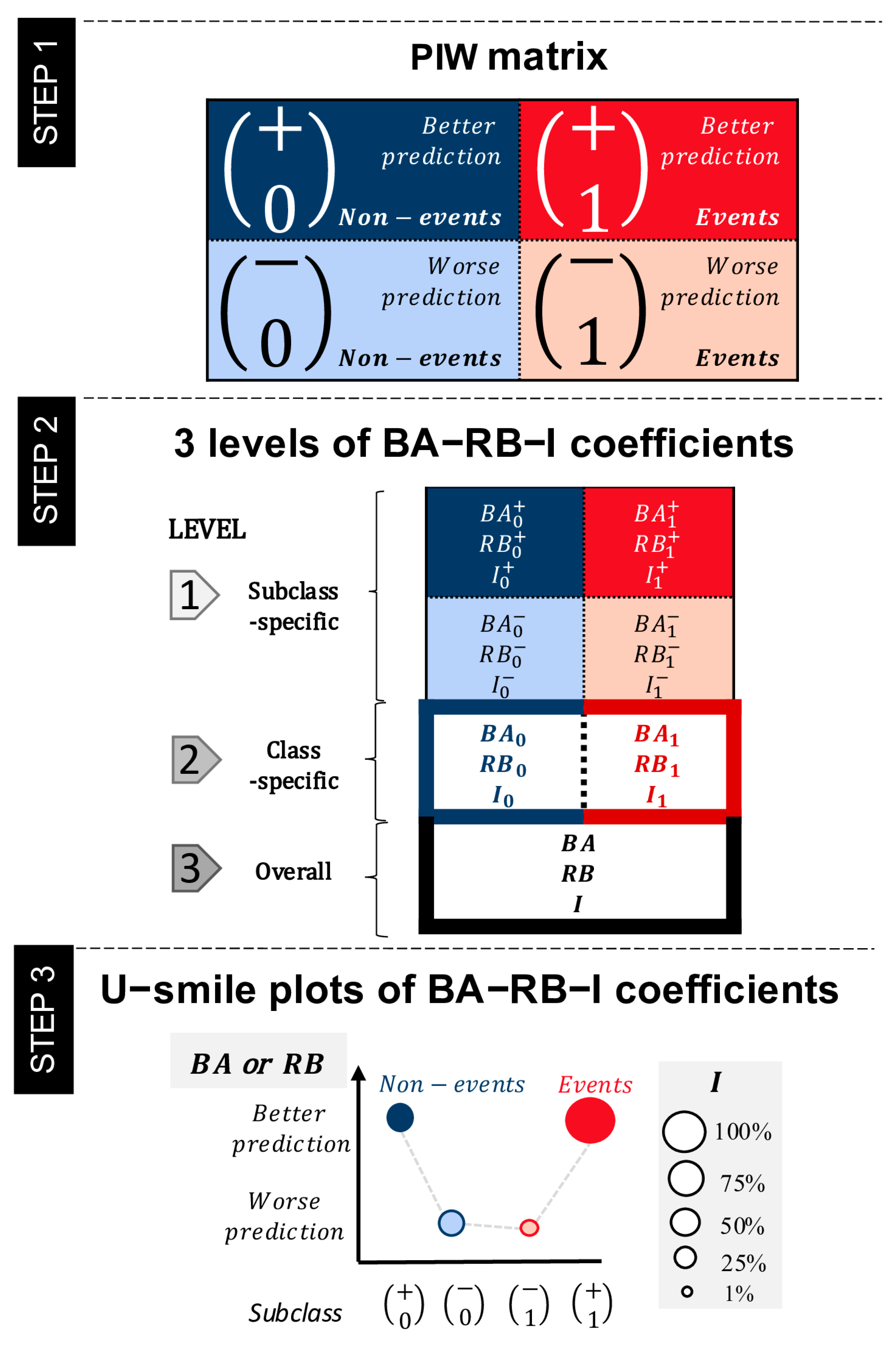
A step-by-step guide to the U-smile method. Superscripts + and − indicate better or worse prediction in the new model compared to the reference model, respectively. Subscripts 0 and 1 refer to the non-event and event outcome classes, respectively. BA coefficients: average absolute changes in prediction between new and reference models; RB coefficients: relative changes in prediction between new and reference models (relative to the prediction error of the reference model); I coefficients: proportions of the prediction changes in each class. The U-smile method evaluates the added predictive value of a candidate variable by comparing residuals (prediction errors) from two nested models: a reference model and a new model that includes the candidate variable. In Step 1, these changes are cross-tabulated with the outcome class (non-event or event) to create a prediction improvement–worsening (PIW) matrix, dividing individuals into four subclasses: non-events with improved prediction (0+), non-events with worsened prediction (0−), events with worsened prediction (1−), and events with improved prediction (1+). Step 2 represents the three-level approach of the U-smile method, i.e., subclass-specific, class-specific, and overall. At level 1, for each subclass, the magnitude of prediction change is quantified as BA and RB coefficients, and the number of individuals in quantified as I coefficients. At level 2, for each class, the net coefficients are defined as differences of the subclass-specific coefficients of level 1, i.e., improvement coefficient less worsening coefficient. At level 3, the weighted overall BA-RB-I coefficients are calculated as weighted means of their respective net coefficients. In Step 3, the U-smile plot of the BA-RB-I coefficients displays the four subclasses along the x-axis and the corresponding BA or RB values on the y-axis. Point color indicates class (blue for non-events, red for events), fill indicates prediction direction (solid for improved, light for worsened), and point size reflects the I coefficient, showing the proportion of affected individuals.
Figure 1.
A step-by-step guide to the U-smile method. Superscripts + and − indicate better or worse prediction in the new model compared to the reference model, respectively. Subscripts 0 and 1 refer to the non-event and event outcome classes, respectively. BA coefficients: average absolute changes in prediction between new and reference models; RB coefficients: relative changes in prediction between new and reference models (relative to the prediction error of the reference model); I coefficients: proportions of the prediction changes in each class. The U-smile method evaluates the added predictive value of a candidate variable by comparing residuals (prediction errors) from two nested models: a reference model and a new model that includes the candidate variable. In Step 1, these changes are cross-tabulated with the outcome class (non-event or event) to create a prediction improvement–worsening (PIW) matrix, dividing individuals into four subclasses: non-events with improved prediction (0+), non-events with worsened prediction (0−), events with worsened prediction (1−), and events with improved prediction (1+). Step 2 represents the three-level approach of the U-smile method, i.e., subclass-specific, class-specific, and overall. At level 1, for each subclass, the magnitude of prediction change is quantified as BA and RB coefficients, and the number of individuals in quantified as I coefficients. At level 2, for each class, the net coefficients are defined as differences of the subclass-specific coefficients of level 1, i.e., improvement coefficient less worsening coefficient. At level 3, the weighted overall BA-RB-I coefficients are calculated as weighted means of their respective net coefficients. In Step 3, the U-smile plot of the BA-RB-I coefficients displays the four subclasses along the x-axis and the corresponding BA or RB values on the y-axis. Point color indicates class (blue for non-events, red for events), fill indicates prediction direction (solid for improved, light for worsened), and point size reflects the I coefficient, showing the proportion of affected individuals.
![Applsci 15 08303 g001]()
Figure 2.
The U-smile plot is a graphical summary of Levels 1 and 2 of the U-smile method. (A) The U-smile plot of the BA or RB coefficients visualizes the effect of adding a new variable to a reference model. The points represent the subclass-specific coefficients of Level 1 of the U-smile method. A smile, a frown, a flat line and a zigzag are the main shapes of the U-smile plot. We observe a double smile (panel a) when the new variable improved prediction in both classes, and a smile + flat line or flat line + smile shape (panels b and c) when the prediction was improved in one class with no changes in the other. Worsened prediction in both classes is indicated by a double frown shape (panel d), and frown + flat line or flat line + frown shapes (panels e and f) show prediction worsening in one class with no changes in the other. A double flat line in the U-smile plot indicates no change in prediction in both classes (panel g), while a zigzag pattern is produced when prediction was improved in one class and worsened in the other (panels h and i). (B) The vertical distances between blue and red points represent class-specific net BA and RB coefficients of Level 2 of the U-smile method and quantify the net effect size of prediction improvement offered by a new marker for non-events and events, respectively.
![Applsci 15 08303 g002]()
Figure 3.
(A) comparative visualization of predictor performance for an informative (ST depression) and a non-informative (glucose) variable added to a reference model, across imbalance range from 1% to 99% of the event class, for the training dataset. The U-smile method enables a swift class-stratified insights, and an immediate identification of an informative variable, overcoming limitations of both ROC curves and SHAP approaches. (A,B) The U-smile plots of the BA and RB coefficients, respectively, show class-stratified usefulness of a candidate predictor added to the reference model. (C) ROC curves for the same models, which do not distinguish class-specific changes. (D) SHAP values for the same models, which indicate feature importance but lack clear class separation.
Table 1.
Effectiveness of the U-smile method across different levels of class imbalance and collinearity between variables.
Table 1.
Effectiveness of the U-smile method across different levels of class imbalance and collinearity between variables.
| Problem Characteristic | Example Use Cases | How Is the U-Smile Method Effective? |
|---|
| Imbalanced scenario |
| Extreme (severe) class imbalance with event (minority) class prevalence ≤ 1% | Rare diseases research, financial fraud detection, IT systems anomalies detection | U-smile method detects prediction improvement in the minority class and reduction in the reference model’s overfitting to the majority class |
| High to moderate class imbalance with event (minority) class prevalence of 10–30% | Predicting post-surgery complications, early detection of machine failures, credit risk assessment | Traditional VS methods are often biased towards the majority class, while the U-smile method can identify variables that are useful for both outcome classes |
| Low class imbalance and class balance with event (minority) class prevalence of 30–50% | Diagnosing prevalent diseases, sentiment analysis (positive vs. negative opinions) | U-smile method’s advantage over traditional methods is less pronounced than under more imbalanced scenarios, but the U-smile method offers more granular insight into prediction changes in each class |
| Collinearity |
| Collinearity between informative variables | Genomic or imaging data where multiple predictors represent overlapping biological processes | U-smile method’s results aligned with LRT. At low-to-moderate correlations (Pearson ≤ 0.3), it identified added value from new informative variables. At moderate-to-high correlations (Pearson 0.4–0.7), plots flatlined, indicating no added value and preventing false-positives. At extreme correlations (Pearson ≥ 0.8), U-smile method reflected the lack of robustness to multicollinearity of both the LRT and the logistic regression model |
| Collinearity between informative and non- informative variables | Administrative health records where proxy variables or redundant features in high-dimensional datasets may correlate with true risk factors | U-smile method, consistently with LRT, avoided falsely labeling correlated but non-informative variables as useful, showing no prediction gain in either class |
Table 2.
Limitations of the U-smile method and directions for further methodological development.
Table 2.
Limitations of the U-smile method and directions for further methodological development.
| Limitations of the U-Smile Method | Direction for Further Methodological Development |
|---|
| The U-smile method has been developed and validated on logistic regression models | Apply the U-smile method to non-linear or non-parametric models, such as decision trees, random forests, or neural networks as the U-smile method is conceptually compatible to any model that produces probability estimates and does not require any model assumptions or affect model training |
| The U-smile method has been developed and validated in the context of nested models that differ by a single variable as this setup reflects many applied use cases (particularly in biomarker, clinical and epidemiological research) | Apply the U-smile method to compare models differing by multiple variables and non-nested models, including models with partially overlapping sets of predictors |
| The U-smile method is currently applied post hoc after model training | Integrate the U-smile method with regularized frameworks like LASSO, ridge or elastic net, automated VS algorithms and stepwise regression |
| The U-smile method has been developed and validated for BC tasks only | Adapt and validate the U-smile method for multiclass classification and time-to-event (survival) outcomes |
| Application of the U-smile method to real-time data may be computationally intensive in very large datasets or high-throughput environments | Optimize algorithmic efficiency through parallel computing approaches or approximate methods |
| The U-smile method has been evaluated on training and test datasets comprising 300 and 100 observations, respectively | Investigate the effect of dataset size on the variability of the BA-RB-I coefficients |
| Disclaimer/Publisher’s Note: The statements, opinions and data contained in all publications are solely those of the individual author(s) and contributor(s) and not of MDPI and/or the editor(s). MDPI and/or the editor(s) disclaim responsibility for any injury to people or property resulting from any ideas, methods, instructions or products referred to in the content. |
© 2025 by the authors. Licensee MDPI, Basel, Switzerland. This article is an open access article distributed under the terms and conditions of the Creative Commons Attribution (CC BY) license (https://creativecommons.org/licenses/by/4.0/).


