A Resilience Quantitative Assessment Framework for Cyber–Physical Systems: Mathematical Modeling and Simulation

Abstract

As cyber threats continue to grow in complexity and persistence, resilience has become a critical requirement for cyber–physical systems (CPSs). Resilience quantitative assessment is essential for supporting secure system design and ensuring reliable operation. Although various methods have been proposed for evaluating CPS resilience, major challenges remain in accurately modeling the interaction between cyber and physical domains and in providing structured guidance for resilience-oriented design. This study proposes an integrated CPS resilience assessment framework that combines cyber-layer anomaly modeling based on Markov chains with mathematical modeling of performance degradation and recovery in the physical domain. The framework establishes a structured evaluation process through parameter normalization and cyber–physical coupling, enabling the generation of resilience curves that clearly represent system performance changes under adverse conditions. A case study involving an industrial controller equipped with a diversity-redundancy architecture is conducted to demonstrate the applicability of the proposed method. Modeling and simulation results indicate that the framework effectively reveals key resilience characteristics and supports performance-informed design optimization.

1. Introduction

Resilience has long been a foundational concept in fields such as urban planning, ecology, and socio-technical systems. It broadly refers to a system’s ability to absorb disturbances, adapt to change, and recover functionality [1]. In recent years, this concept has been extended to the field of cybersecurity, resulting in the notion of cyber resilience. Unlike natural or social disruptions, cyber threats are often stealthy, adaptive, and recurrent, making cyber resilience distinct in both scope and focus from traditional resilience paradigms. Cyber resilience refers to a system’s ability to anticipate, withstand, recover from, and adapt to adverse conditions—including cyber attacks and system compromises—while continuing to perform essential functions. Unlike traditional security approaches that focus primarily on attack prevention, resilience emphasizes operational continuity during compromised states and the ability to recover within acceptable timeframes. The concept of cyber resilience has attracted growing attention across multiple disciplines, particularly in the context of cyber–physical systems (CPSs) that support critical infrastructures such as power grids, industrial control systems (ICSs), and transportation networks [2]. As CPSs become increasingly interconnected and vulnerable to sophisticated threats, resilience has shifted from being a desirable property to a fundamental requirement for ensuring system dependability and mission assurance [3].

In CPSs, resilience must be considered holistically across both the physical and cyber domains. Physical components, such as sensors and actuators, interact closely with cyber elements, including communication protocols, data links, and control algorithms. These interactions create tightly coupled dependencies, so cyber disruptions—whether caused by malicious attacks or accidental faults—can propagate into the physical domain, affecting system performance and safety [4]. To support robust system design and operational planning, it is essential to develop rigorous methods for quantifying CPS resilience in the face of such disruptions.

Despite the growing consensus on the critical importance of cyber resilience in CPSs, significant challenges remain in quantitatively evaluating resilience and designing CPSs that are resilient by construction. These challenges arise from several core issues. From an evaluation perspective, resilience is a system-level property that lacks a unified definition and is often described too broadly, making it difficult to measure consistently [5]. From a design perspective, strategies to achieve resilience—such as redundancy, fault tolerance, adaptive control, and cyber defense—are diverse and hard to integrate within a single framework [6]. In CPSs specifically, the added complexity of cyber–physical coupling introduces a third challenge: the lack of an integrated modeling strategy for representing resilience processes across both the cyber and physical domains [7].

A variety of methods have been proposed to assess the cyber resilience of systems, as illustrated in Figure 1. These methods can be broadly categorized into four types: (1) static assessment metrics, such as availability, risk indexes, and reliability indicators, which provide high-level summaries but fail to capture dynamic system behavior; (2) red-teaming and adversarial simulation, which enable exploratory analysis and scenario testing, but often lack analytical generality and repeatability; (3) dynamic performance modeling, which focuses on time-dependent degradation and recovery in the physical domain, but frequently overlooks cyber-layer processes; and (4) cyber-layer security models, including attack graphs, stochastic processes, and game-theoretic approaches, which describe adversarial behaviors and defense mechanisms, typically in isolation from physical impacts. A detailed review of these approaches and their representative studies is provided in Section 2.

While each of these methods contributes valuable insights, most either concentrate on a single domain or lack integration across the CPS architecture. A key missing element is a unified, mathematically grounded framework that accounts for both the dynamics of performance degradation and the stochastic nature of cyber faults or attacks. Such a framework should not only model temporal system behavior under adverse conditions but also support the design and validation of resilient system architectures. Addressing this gap forms the motivation of this paper.

This study presents an integrated framework for evaluating cyber resilience in cyber–physical systems by combining dynamic performance modeling in the physical domain with probabilistic security modeling in the cyber layer. The approach bridges the gap between physical performance degradation and cyber-layer disruptions, enabling a unified and quantitative analysis of system-level resilience under adversarial conditions. The key contributions are as follows:

• We develop a diversity-redundancy security architecture tailored to CPSs, incorporating heterogeneous execution units, voting mechanisms, fault isolation, and dynamic recovery. A Markov process model captures probabilistic transitions among cyber states—operational, degraded, detectable failure, and undetectable failure—under persistent threats.
• We formulate a dynamic model that describes the system’s functional evolution in response to cyber disturbances. This model quantifies resilience metrics such as degradation rate, recovery capacity, and long-term steady-state behavior.
• We introduce a segmentation-weighted coupling method that aligns cyber-state sequences with corresponding physical performance phases. By weighting these segments according to their duration and stationary probabilities, the framework supports consistent and interpretable resilience evaluation.
• A case study involving an ICS demonstrates the framework’s effectiveness in comparing design alternatives and identifying critical resilience parameters.

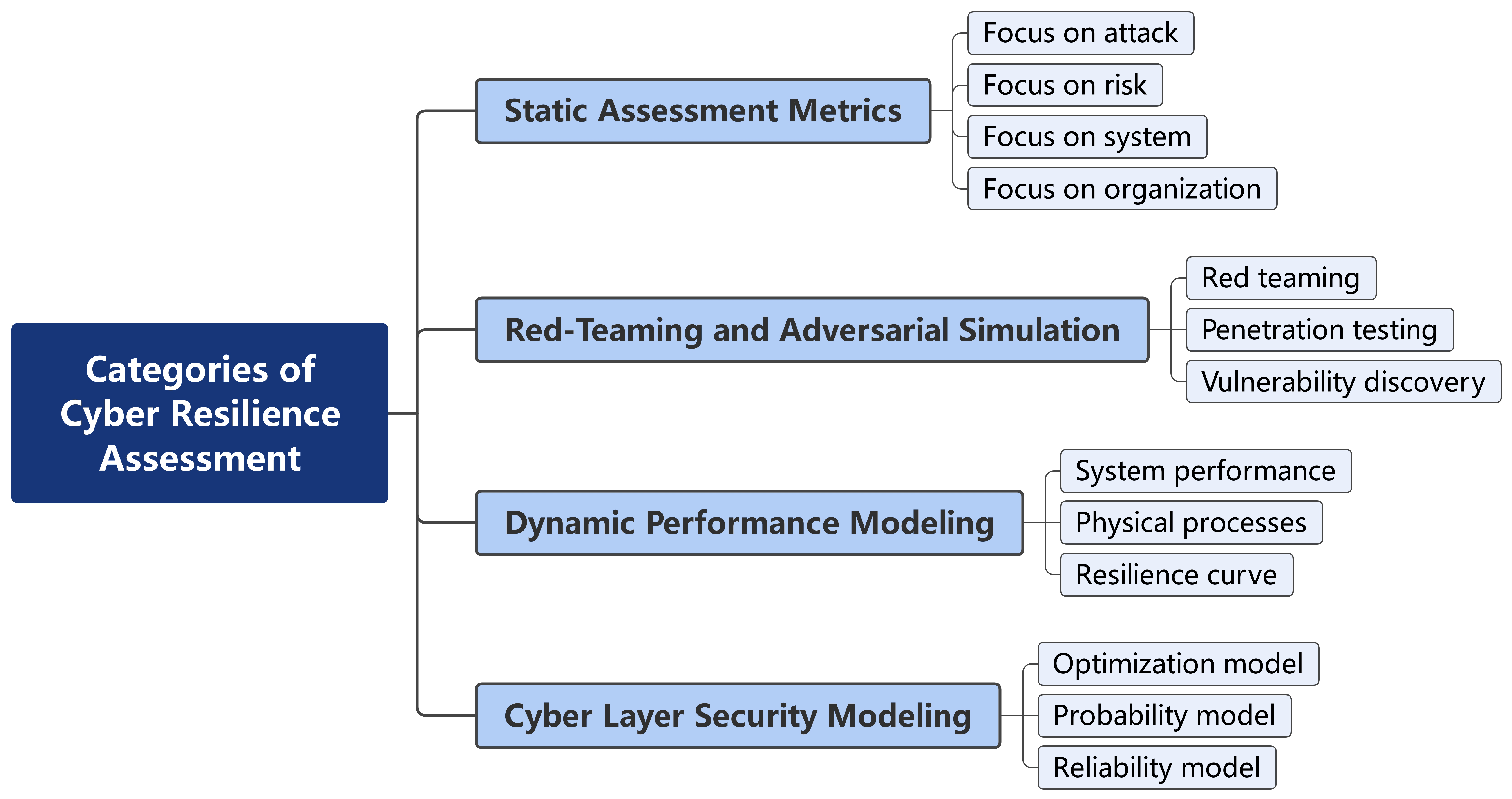
The remainder of this paper is organized as follows. Section 2 reviews related work on cyber resilience evaluation methods. Section 3 presents the proposed evaluation framework, including the security architecture, stochastic modeling, performance dynamics, and the cyber–physical coupling strategy. Section 4 provides a case study to validate the framework and demonstrate its practical value. Finally, Section 5 concludes this paper and discusses directions for future research.

2. Related Work

Cyber resilience has become a central concern in CPS research, especially under persistent adversarial threats. Numerous approaches have been developed to evaluate and enhance resilience, drawing from both the cyber and physical domains. Building on the classification introduced in the Introduction, this section reviews representative studies across four categories of cyber resilience assessment, highlighting their methodological foundations and practical applicability.

2.1. Static Assessment Metrics

Static resilience metrics quantify a system’s resilience based on predefined structural, organizational, or procedural characteristics. These metrics are often derived from standards, expert consensus, or structured frameworks, and are typically expressed through indicators such as availability, reliability, risk indexes, or system-level resilience scores [8,9]. They offer an accessible way to compare systems or assess baseline resilience levels without requiring complex modeling or simulation.

A prominent example is the guidance provided by the U.S. National Institute of Standards and Technology (NIST). In Special Publication 800-160 [10], NIST outlines a systems engineering approach to developing cyber resilient systems, emphasizing resilience objectives, design principles, and traceable metrics across system layers. This methodology builds on earlier work by MITRE [11,12], which formalized structured goals and trade-space analysis in resilience engineering. Building upon these foundations, NIST also released SP 800-82 [13], a guide focused on operational technology security in ICSs. It incorporates static metrics aligned with the widely adopted Cybersecurity Framework [14], covering categories such as governance, detection, and recovery.

Similar initiatives have been introduced globally. The United Kingdom’s National Cyber Security Centre proposed a Cyber Resilience Assessment Framework for critical infrastructure [15]. The European Union incorporated cyber resilience objectives in the NIS2 Directive [16], while China issued cyber resilience evaluation criteria targeting national information infrastructure [17].

While these metrics provide a clear structure and facilitate benchmarking, they are limited in capturing dynamic system behavior or adapting to evolving threats. They often represent high-level abstractions that may overlook internal system complexity or cross-domain interactions. As a result, static metrics are best suited as foundational tools or for compliance purposes, rather than as standalone resilience evaluation strategies.

2.2. Red-Teaming and Adversarial Simulation

Red-teaming and adversarial simulation have become increasingly common approaches to evaluating cyber resilience through emulated attacks and exploratory defense testing. Originating in military practice, these methods are now widely used to assess the resilience of mission-critical systems and national infrastructure. The core concept involves deploying a red team acting as a simulated attacker to probe system vulnerabilities in a controlled environment [18]. This process helps identify hidden weaknesses, evaluate operational robustness, and test defense mechanisms under near-realistic conditions [19]. Organizations such as the RAND Corporation have published practical guidelines for conducting red-team exercises in defense and critical infrastructure contexts [20].

Recent efforts have enhanced the rigor of red-teaming by integrating structured adversarial taxonomies, such as the MITRE ATT&CK framework [21]. This integration supports more systematic and repeatable simulations by linking specific threat techniques to known system vulnerabilities [22,23]. As a result, red-teaming can better inform threat-aware defense strategies and connect theoretical resilience concepts with practical system exposures.

Despite their realism, red-teaming exercises have notable limitations. Results often depend heavily on the specific attack vectors, tools, and tactics used, limiting generalizability and repeatability. Furthermore, the effectiveness of such evaluations may vary across systems and environments, making it difficult to establish standardized benchmarks for resilience.

2.3. Dynamic Performance Modeling

This class of approaches assesses cyber resilience by examining how system functionality changes over time in response to adverse conditions. Rather than focusing on component-level faults or security-specific metrics, these methods adopt a system-level, mission-oriented view of resilience [24,25]. As elaborated in [26], this has been referred to as the “System Performance Perspective,” where resilience is measured by tracking performance trajectories across key stages.

This perspective is especially relevant to CPSs, where physical processes respond dynamically to cyber-layer disturbances. For instance, a study developed resilience assessment frameworks for fast-response CPS scenarios, modeling the thermal runaway behaviors of industrial systems under cyber attacks [27]. Several studies have proposed evaluation workflows using this perspective in the context of power grids or smart energy systems, demonstrating resilience curves in simulation environments [28,29]. Additional research has focused on IT infrastructure, proposing quantitative methods to evaluate resilience via scenario-based attack-response simulations [30]. More recent efforts also introduced more structured resilience metrics for CPSs, capturing dynamic system responses to cyber intrusions over time [31,32,33].

While these methods offer interpretable and mission-relevant insights, they often rely on domain-specific performance indicators and physical failure models. As a result, their applicability may vary across different systems. Additionally, most models emphasize the physical domain while omitting explicit representations of cyber-layer processes or stochastic attack progression. Capturing cyber–physical interactions in an integrated and scalable manner remains a challenge in this line of research.

2.4. Cyber-Layer Security Modeling

Cyber-layer security modeling focuses on representing adversarial behavior, system vulnerabilities, and defense strategies through formal analytical methods. Common tools include attack graphs [34], stochastic Petri nets [35], Markov models [36,37], game-theoretic frameworks [38], and Bayesian networks [39], etc. These methods support probabilistic analysis of cyber risks, identification of critical nodes, and evaluation of system security under varying threat scenarios. Their primary strength lies in capturing uncertainty, intent, and interaction within cyber processes.

Despite their analytical rigor, these models often operate in isolation from the physical layer. They typically do not account for how cyber incidents propagate to affect physical performance or safety. As a result, their applicability to CPSs is limited. Simplifying assumptions—such as static network topologies or security controls for specific types of attacks [40,41]—can further reduce realism and applicability. Without explicit integration of cyber and physical domains, such models cannot offer a complete representation of system resilience.

Overall, each of the four categories reviewed provides valuable insight into specific aspects of cyber resilience. However, they also exhibit inherent limitations, particularly in addressing the interdependence of cyber and physical processes. To address this gap, the following sections present an integrated modeling framework that jointly considers security dynamics in the cyber layer and performance degradation in the physical domain.

3. CPS Resilience Quantitative Assessment Framework

3.1. Quantitative Assessment Framework for Cyber–Physical Coupling

The proposed framework integrates modeling approaches from both the physical and cyber domains to capture the dynamic evolution of CPS performance under cyber attacks. It comprises two primary components:

• Physical domain modeling: This component mathematically represents system performance degradation and recovery, reflecting real-time resilience behavior in response to disruptions.
• Cyber-layer modeling: This component uses a Markov-based stochastic process to capture the impact of cyber attacks and evaluate the effectiveness of heterogeneous redundancy strategies.

By combining these two domains, the framework enables a comprehensive and quantifiable assessment of CPS resilience. Beyond evaluation, it also provides insights to guide the design and optimization of resilient architectures. An overview of the framework is illustrated in Figure 2.

3.2. Physical Domain: System Performance Modeling

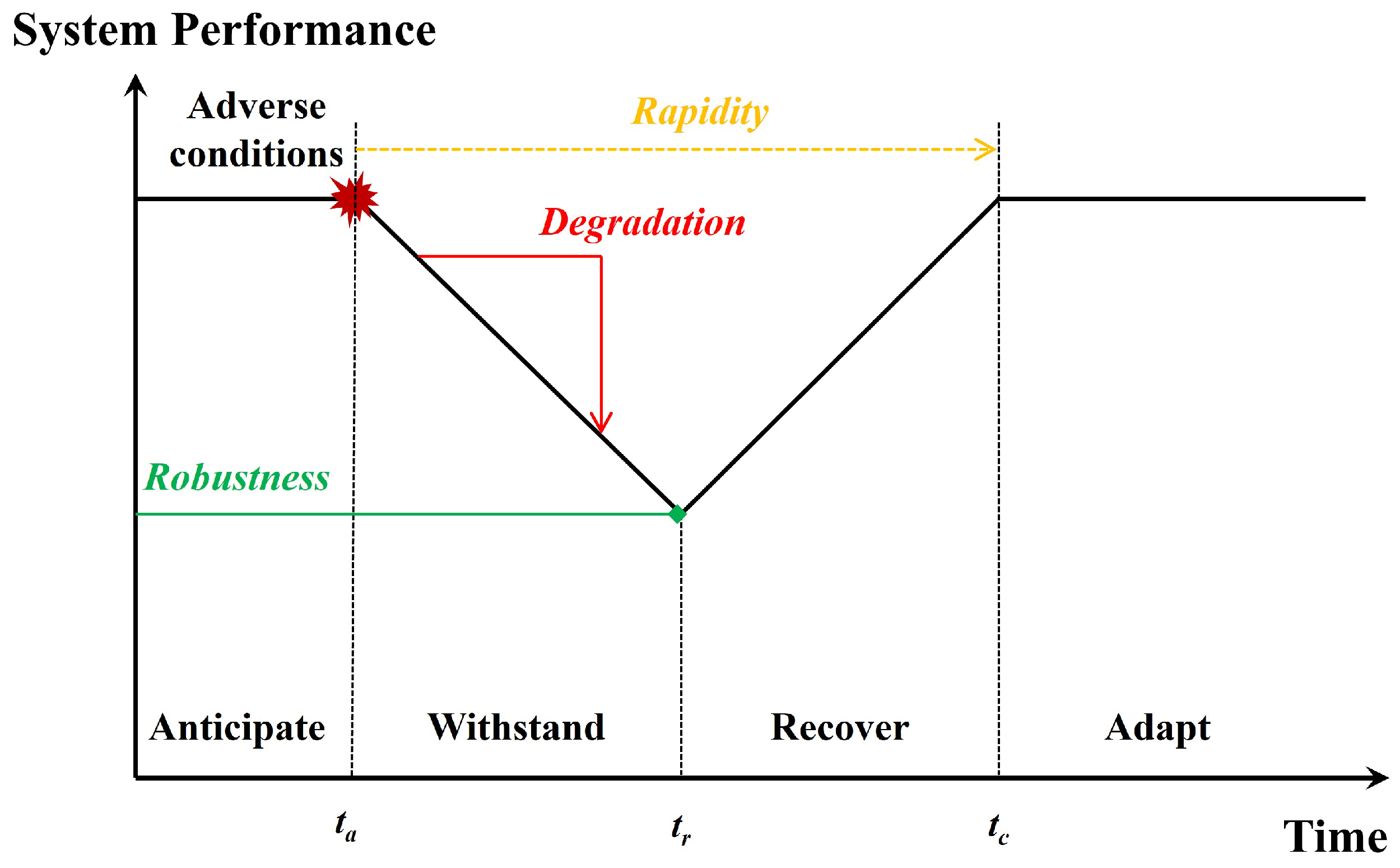
3.2.1. Performance Curve and Resilience Stages

This section discusses the stages and quantitative assessment methods of CPS resilience from the perspective of system performance. In the context of cyber resilience, a system’s ability to recover to an acceptable performance level following degradation is a key indicator of its overall resilience. Such degradation may result from random natural failures—as studied in traditional reliability engineering—or from deliberate cyber attacks.

System performance over time is commonly represented by a performance curve, which depicts how key performance indicators evolve in response to disruptions and recovery efforts. This curve provides a temporal profile of system behavior, capturing both the immediate impact of adverse events and the subsequent restoration trajectory. A typical performance curve for a disrupted system is illustrated in Figure 3, showing the temporal response of a disrupted system. Based on this curve, the resilience process can be divided into four key stages:

• Prevention Stage: The system operates under normal conditions, employing measures such as intrusion detection, anomaly monitoring, and system hardening to maintain stable performance and minimize exposure to threats.
• Withstanding Stage: Under adverse conditions, performance begins to degrade. The system’s ability to maintain partial functionality during this phase reflects its robustness and fault tolerance.
• Recovery Stage: Following the disruption, the system engages recovery mechanisms—such as redundancy activation, reconfiguration, or manual intervention—to restore performance. The speed and efficiency of this process are key resilience indicators.
• Adaptation Stage: The system adjusts to the new environment by updating configurations, learning from the incident, or strengthening defenses. This adaptive capacity supports long-term resilience enhancement.

These stages form the basis for understanding resilience as a time-dependent, performance-driven process. Common metrics include the area under the performance curve, recovery time, and minimum performance during disruption. Such indicators provide an intuitive means of comparing resilience across systems and scenarios.

However, most existing approaches generate performance curves through experiments or simulations based on physical control models. While effective in specific contexts, these methods are often system-specific and highly dependent on the chosen performance indicators. They typically lack a unified modeling framework and struggle to account for the complex interdependence between cyber and physical domains in CPSs.

To overcome these limitations, the next subsection presents a mathematical modeling approach for generating generic performance curves. This model also lays the groundwork for integrating physical dynamics with cyber-layer disruptions.

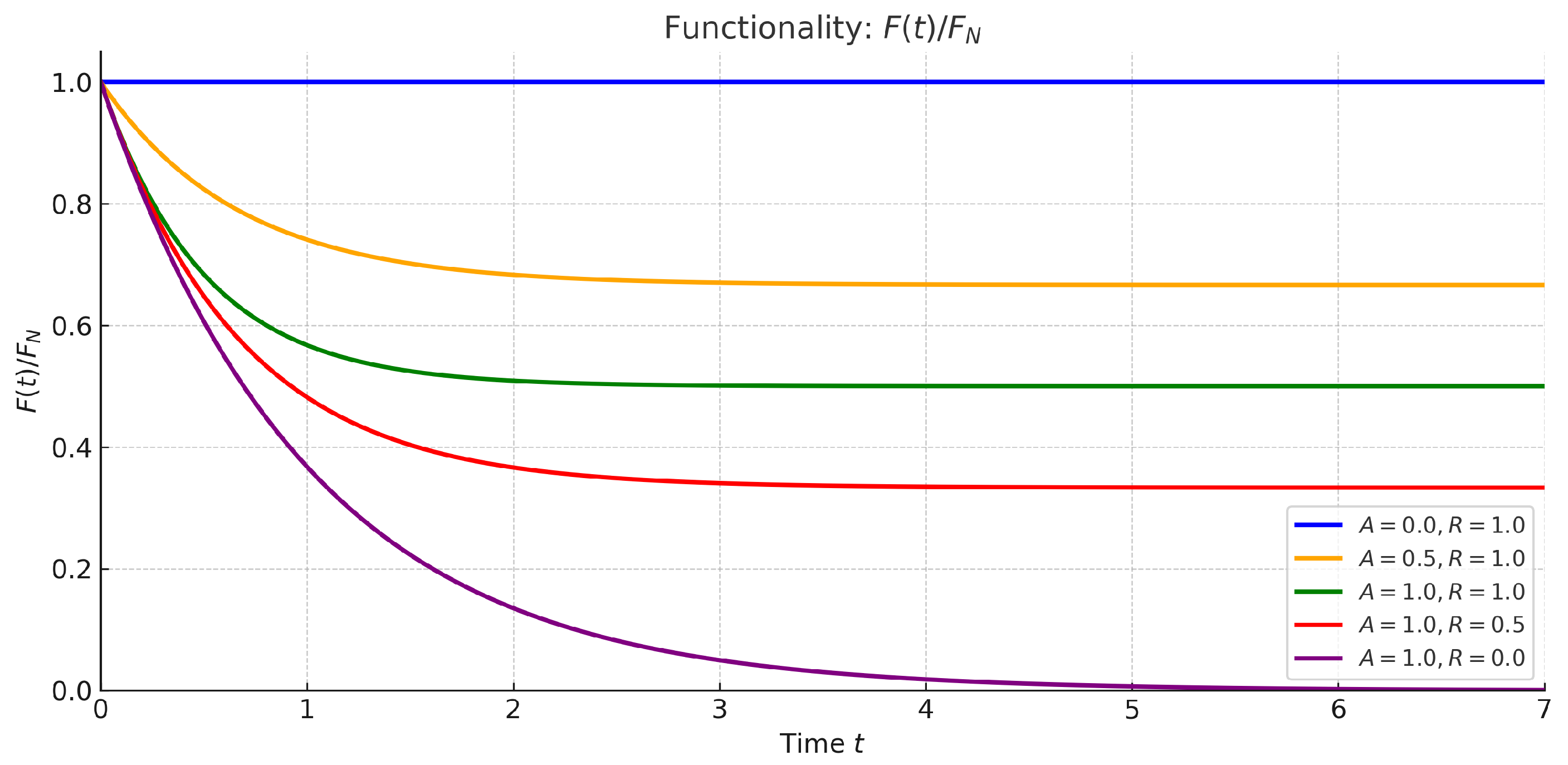
3.2.2. CPS Resilience Mathematical Modeling

In this section, a mathematical model is proposed to simulate the dynamic behavior of system performance under adverse events. CPSs are designed to fulfill one or more functional objectives. We postulate that for a given task or mission, there exists a function $M\left(t\right)$ that represents the accomplishment of that mission, cumulative from the mission start time $t_0$ up to the current time t. The derivative of $M\left(t\right)$ with respect to time, denoted as $F\left(t\right)$, reflects the system’s instantaneous performance level and thus serves as the basis for the performance curve. The relationship between $M\left(t\right)$ and $F\left(t\right)$ can be expressed as follows:

$$\begin{array}{c}F\left(t\right)={\displaystyle \frac{dM}{dt}}\hfill \\ M\left(t\right)={\int }_{t_0}^{t}F\left(\tau \right)d\tau \hfill \end{array}$$

(1)

Under normal conditions, and in the absence of any disruptive events, system performance may vary slightly over time due to operational dynamics. However, for simplicity of analysis, we assume that the nominal performance remains constant and express it as $F_N\left(t\right)=F_N$. This assumption allows us to focus on how adverse events affect performance deviation and recovery behavior, forming the basis for resilience modeling.

Next, we define a control equation that governs the evolution of the performance curve by capturing both degradation and recovery dynamics. As a first-order approximation, we assume that the adverse event reduces performance at a constant rate, while the recovery process is linearly proportional to the performance loss relative to the nominal level.

Under these assumptions, the rate of change in performance $F\left(t\right)$ can be described as follows [42]:

$${\displaystyle \frac{dF}{dt}}=-A\left(t\right)F\left(t\right)+R\left(t\right)\left[F_N-F\left(t\right)\right]$$

(2)

where $A\left(t\right)$ represents the impact caused by adverse events and $R\left(t\right)$ represents the impact on system recovery capability.

Let $Q\left(t\right)=A\left(t\right)+R\left(t\right)$; then the equation can be simplified as follows:

$${\displaystyle \frac{dF}{dt}}+Q\left(t\right)F\left(t\right)=+F_{N}R\left(t\right)$$

(3)

This differential equation has a general solution as follows:

$$F\left(t\right)=exp\left[-{\int }_0^{t}Q\left(p\right)dp\right]\left[F\left(0\right)+F_N{\int }_0^{t}R\left(\tau \right)e^{{\int }_0^{\tau }Q\left(p\right)dp}d\tau \right]$$

(4)

To better understand the model, we analyze three representative cases based on the system parameters A and R.

A.

Constant-coefficient model

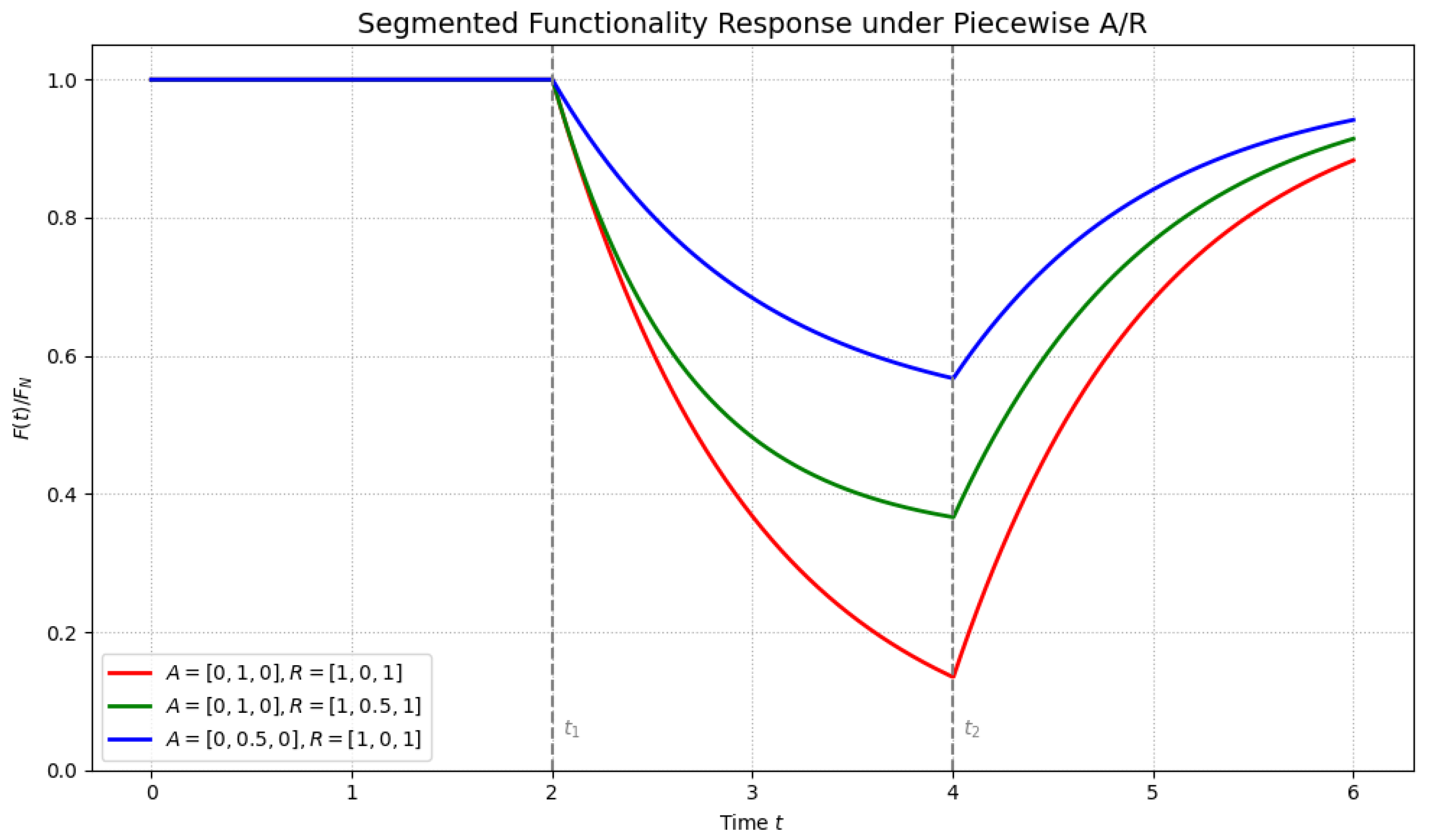
Both A and R are assumed as time-invariant constants. This simplified assumption reflects a scenario in which the disturbance intensity and the system’s recovery capability remain constant over time. Under this assumption, the solution is

$$F\left(t\right)=\left[F\left(0\right)-{\displaystyle \frac{F_{N}R}{Q}}\right]e^{-Qt}+{\displaystyle \frac{F_{N}R}{Q}}$$

(5)

where $F\left(0\right)$ represents the initial condition of F.

As $t\to \infty$, the performance $F\left(t\right)$ approaches a steady-state value:

$$F_{\infty }=\underset{t\to \infty }{lim}F\left(t\right)=F_N{\displaystyle \frac{R}{A+R}}$$

(6)

Figure 4 illustrates the evolution of system performance over time under the constant-coefficient model. In general, the trajectory of the performance curve is determined by the relative strength of the adverse impact and recovery capacity, as well as the system’s initial condition. When the system starts at nominal performance and the adverse effect dominates recovery, the performance exhibits exponential decay. Conversely, if the initial performance is low and the recovery effect outweighs the adverse impact, the system will gradually recover.

This basic form captures the fundamental resilience dynamics where the system degrades at a steady rate and recovers proportionally to the performance gap. Although simplistic, this model provides clear insights into baseline resilience behavior and serves as a reference point for analyzing more complex dynamics in later sections.

B.

Piecewise constant-coefficient model

Building upon the constant-coefficient model, we now consider the case where the effects of adverse events and recovery capabilities change at certain points in time. In this scenario, the system transitions between different phases, each defined by a distinct pair of constant values for the adverse factor A and the recovery factor R. This results in a piecewise-constant model.

At each phase, $\mathbf{A}$ and $\mathbf{R}$ are defined as $\mathbf{A}=\left(A_1,A_2,\dots A_n\right)$, $\mathbf{R}=\left(R_1,R_2,\dots R_n\right)$. The model can be expressed mathematically as follows:

$${\displaystyle \frac{d{F}_i}{dt}}=\left[F_N-F\left(t\right)\right]R_i-F\left(t\right)A_i$$

(7)

Accordingly, the solution to the model takes the form of a piecewise function, where in each time interval $t_n$, the solution corresponds to a particular form derived from Equation (5). Figure 5 shows a representative performance curve generated by the piecewise-constant model, illustrating changes in the system trajectory as A and R shift between discrete intervals.

This approach allows for modeling scenarios such as escalating attacks or staged recovery strategies, where control mechanisms or external conditions shift over time—for example, transitioning from manual to automated recovery. It adds realism to the simulation while keeping analytical complexity at a tractable level.

C.

Linear (or piecewise linear) coefficient model

Extending the model further, we assume that the adverse factor A(t) and the recovery factor R(t) are linear or piecewise linear functions of time, such as $A\left(t\right)=\alpha +\beta t$, $R\left(t\right)=\mu +\nu t$. Under this assumption, the system’s performance equation becomes

$${\displaystyle \frac{dF}{dt}}+\left[\left(\alpha +\mu \right)+\left(\beta +\nu \right)t\right]F\left(t\right)=+F_N\left(\mu +\nu t\right)$$

(8)

The solution to the model can be expressed in terms of the error function. As the general solution has already been provided in Equation (4), it will not be repeated here. The piecewise linear model introduces time-varying coefficients, resulting in a smoother and more flexible performance curve.

3.2.3. Extension to Time-Varying Dynamics and Physical Interpretations

The proposed mathematical model for performance evolution offers an abstract and flexible framework. In the previous subsection, we examined system behavior under constant, piecewise-constant, and time-linear forms of degradation and recovery rates. This subsection explores potential extensions to time-varying formulations and their corresponding physical interpretations.

Given the realities of evolving threats, environmental fluctuations, and system aging, real-world CPSs often exhibit failure and recovery rates that are time-dependent or context-sensitive. Accordingly, A and R can be naturally extended to time-varying functions $A\left(t\right)$ and $R\left(t\right)$, allowing the model to capture more complex and realistic dynamics under varying operational conditions.

In practical applications, the temporal evolution of these parameters can reflect the control laws and physical characteristics inherent to specific CPS domains. For instance, in a water-level control system, degradation and recovery rates may remain constant under nominal conditions but may gradually vary linearly with time due to valve wear or sensor drift. In contrast, in energy storage systems such as supercapacitors or batteries, performance degradation may follow a quadratic trend over time, capturing the nonlinear accumulation of charge or discharge dynamics. Furthermore, in temperature regulation within chemical reactors, degradation and recovery rates may evolve exponentially, reflecting nonlinear heat transfer behavior and delayed actuator response under thermal stress. This modeling flexibility allows the abstract formulation to approximate the underlying differential equations that govern the physical processes of diverse CPSs.

The piecewise-constant form adopted in this work provides a tractable and intuitive approximation. From a modeling perspective, both time-invariant and time-varying representations ultimately require parameter estimation for $A\left(t\right)$ and $R\left(t\right)$; therefore, this assumption does not compromise the generality of the approach. By isolating stages such as degradation, stability, and recovery, this approach effectively reveals key system behaviors while preserving analytical simplicity.

In Section 3.3, we will incorporate this physical domain model with a Markov-based cyber-layer model to construct a unified resilience assessment framework. Note that extending the framework to support continuously time-varying functions is a promising direction for future work. In particular, integrating such extensions with richer cyber-layer models, such as Bayesian networks or game-theoretic approaches—can further enhance the fidelity and applicability of resilience assessment in complex CPS environments.

3.3. Cyber Layer: Security Architecture and Modeling

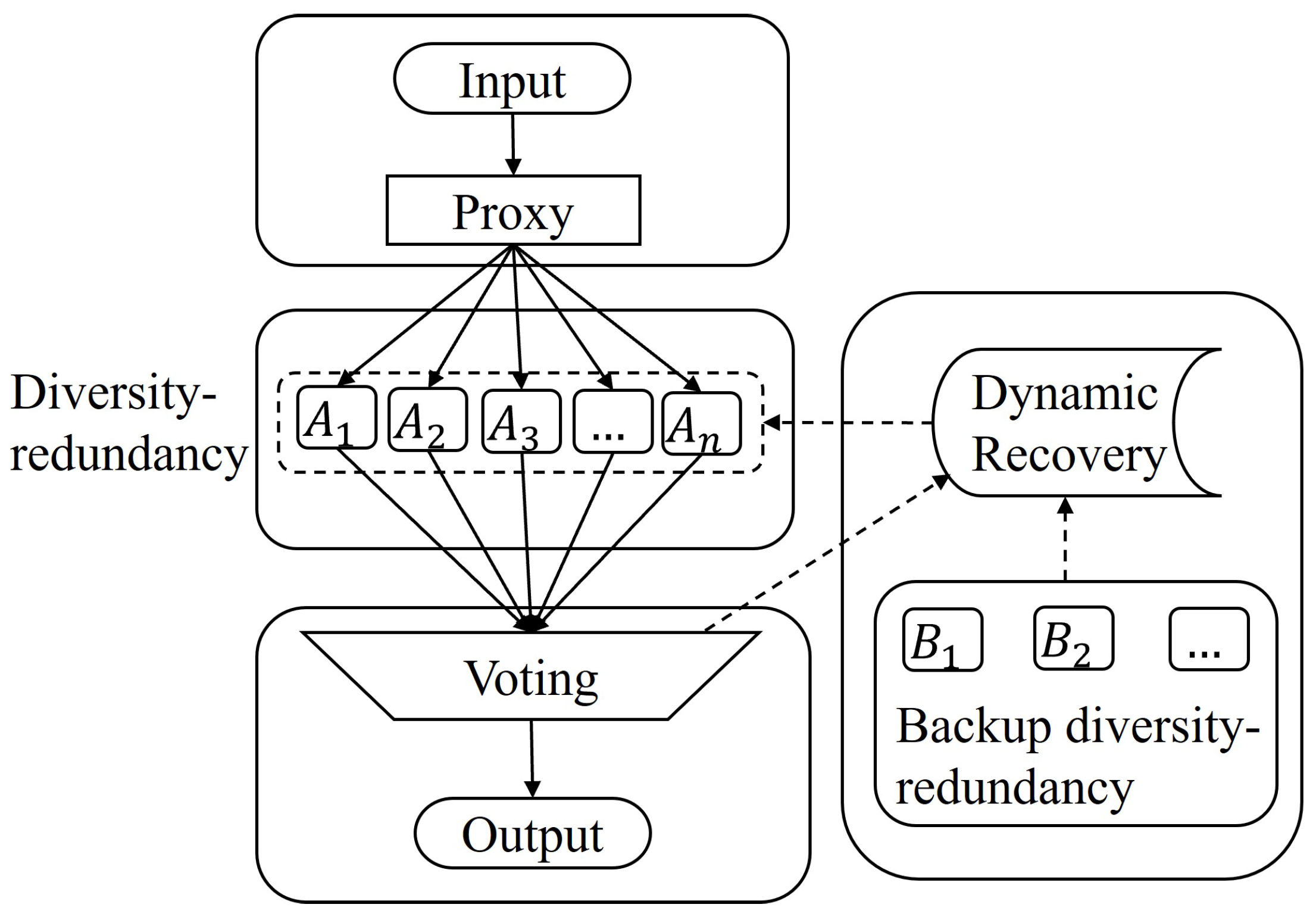
3.3.1. Diversity-Redundancy Security Architecture

Redundancy is a widely adopted strategy in CPSs to improve fault tolerance and enhance system dependability. Traditional architectures typically employ homogeneous redundancy, relying on identical components, such as controllers or software instances, to provide backup functionality during failures.

However, against increasingly sophisticated and stealthy cyber threats, a single exploit targeting a shared weakness can simultaneously compromise all homogeneous redundant units, undermining the intended fault tolerance and severely weakening system resilience.

To address the limitations of homogeneous redundancy in the face of advanced cyber threats, we propose a diversity-redundancy security architecture that incorporates voting and recovery mechanisms. This design targets critical components such as industrial controllers, information transmission units, and supervisory control elements, which often serve as attack surfaces in CPS environments.

As shown in Figure 6, the architecture integrates four core functional modules: diverse redundancy, voting awareness, fault isolation and failover, and dynamic recovery. These modules work together to improve the system’s ability to detect, contain, and recover from cyber-induced faults or intrusions in a timely and autonomous manner. The key features of the proposed architecture are summarized as follows:

• Diverse Redundancy: Multiple redundant units are deployed using heterogeneous implementations (e.g., different hardware platforms, operating systems, or control logic), minimizing the risk of simultaneous compromise due to shared vulnerabilities.
• Voting Awareness: A runtime majority voting mechanism monitors the output consistency of redundant units. Discrepancies are used as indicators of possible compromise or malfunction, serving as an early warning mechanism.
• Fault Isolation and Failover: Upon detection of abnormal behavior, the compromised node is automatically isolated. Control responsibilities are seamlessly handed over to a healthy redundant unit, ensuring uninterrupted operation.
• Dynamic Recovery: The isolated node enters a secure recovery mode, where it is re-initialized using trusted baseline images or reconfigured through remote attestation and software refresh, before being reintegrated into the redundant pool.

This architecture not only enhances fault tolerance but also embeds adaptability and self-healing capabilities—hallmarks of cyber resilience. It is particularly suited for high-assurance CPS environments where sustained functionality under adversarial conditions is critical.

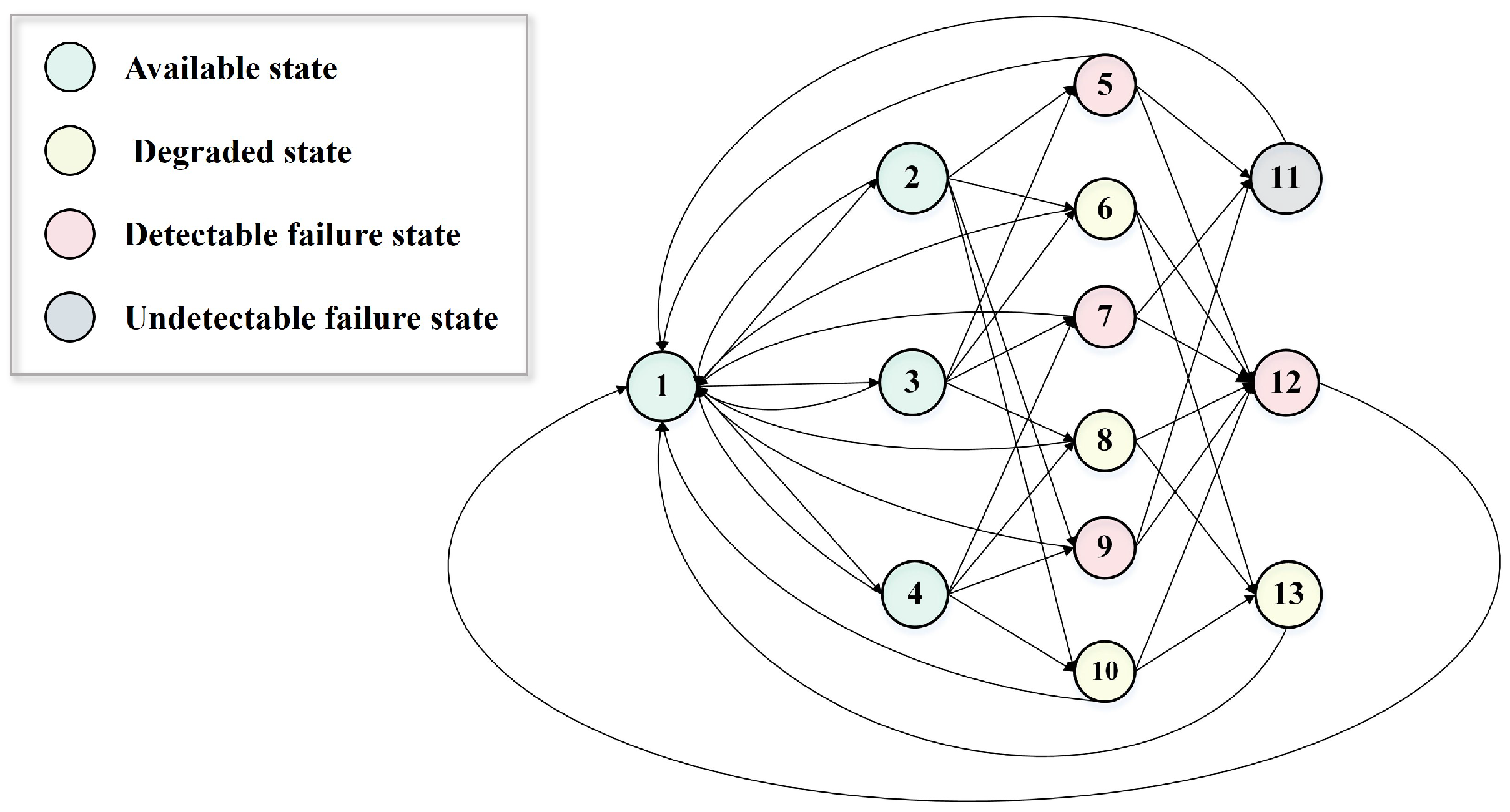
3.3.2. Markov Process Modeling

Based on the diversity-redundancy security architecture introduced in the previous section, we construct a Markov model to describe the probabilistic behavior of the system under sustained cyber threats.

We consider a setting in which three redundant execution units (e.g., controllers, processing modules, or computing nodes) operate in parallel within the CPS. The system output is determined through majority voting. If an inconsistency is detected among the execution results, the system initiates fault isolation and failover and engages in dynamic recovery procedures targeting the abnormal units.

Under this architecture, the state space of the system can be defined based on the functional status of the individual execution units after experiencing cyber attacks. Specifically, when the majority of execution units remain operational, the system is considered available. Conversely, unfavorable states include degraded and failed modes, which can be further divided into detectable (aware) and undetectable (unaware) categories, depending on whether inconsistencies in outputs are observable. The system states are defined as follows:

• Available state: The majority of execution units are functioning correctly.
• Degraded state: The majority of execution units have failed, and their outputs are inconsistent.
• Detectable failure state: The majority of units have failed, but their outputs are consistent, allowing detection.
• Undetectable failure state: All execution units have failed and generate identical (erroneous) outputs, leading to a silent failure.

Based on the above classification, we construct a continuous-time Markov chain (CTMC) model for the proposed diversity-redundancy security architecture. As shown in Figure 7, the model consists of 13 distinct steady states. Among them are the following:

• States 1–4 represent system availability.
• States 5, 7, 9, 12, and 13 represent detectable failures.
• States 6, 8, and 10 correspond to degraded but observable states.
• State 11 denotes the undetectable failure (stealthy failure) state.

The model’s transitions are governed by several parameters, including the following:

• ${\lambda }_i$: Failure rate of the i-th execution unit due to cyber attack-induced disruption.
• ${\mu }_1$: Mean time to recovery when one unit fails with abnormal output.
• ${\mu }_2$: Recovery rate when two units fail with consistent abnormal output vectors (which may include functional outputs, alerts, performance metrics, etc.).
• ${\mu }_3$: Recovery rate when all three units fail and produce identical abnormal outputs—indicating an undetectable, stealthy failure.
• ${\mu }_4$: Recovery rate when all three units fail but their outputs are mutually inconsistent—resulting in an observable degraded state.
• $\sigma$: The uncertainty coefficient that quantifies the likelihood of abnormal output consistency among failed execution units. It reflects how often two faulty nodes produce the same incorrect output vector under adverse conditions.

To evaluate the resilience of the proposed architecture under persistent cyber threats, we solve the steady-state probabilities of the CTMC model introduced above. Assuming that the transition times between states follow exponential distributions, we define the steady-state probability vector as $\mathbf{P}=\left[p_1,p_2,\dots ,p_{13}\right]$, where $p_i$ denotes the long-run probability of the system being in state i. Based on the state transition diagram (Figure 7) and transition matrix ${\mathbf{T}}_{\mathbf{ij}}$ (

Table 1. The transition matrix of the CTMC model.

State	$S_1$	$S_2$	$S_3$	$S_4$	$S_5$	$S_6$
$S_1$	$-{\lambda }_1-{\lambda }_2-{\lambda }_3$	${\lambda }_1$	${\lambda }_2$	${\lambda }_3$	0	0
$S_2$	${\mu }_1$	$-{\mu }_1-{\lambda }_2-{\lambda }_3$	0	0	${\lambda }_2\sigma$	${\lambda }_2(1-\sigma )$
$S_3$	${\mu }_1$	0	$-{\mu }_1-{\lambda }_3-{\lambda }_1$	0	${\lambda }_1\sigma$	${\lambda }_1(1-\sigma )$
$S_4$	${\mu }_1$	0	0	$-{\mu }_1-{\lambda }_2-{\lambda }_1$	0	0
$S_5$	${\mu }_2$	0	0	0	$-{\lambda }_3-{\mu }_2$	0
$S_6$	${\mu }_4$	0	0	0	0	$-{\lambda }_3-{\mu }_4$
$S_7$	${\mu }_2$	0	0	0	0	0
$S_8$	${\mu }_4$	0	0	0	0	0
$S_9$	${\mu }_2$	0	0	0	0	0
$S_{10}$	${\mu }_4$	0	0	0	0	0
$S_{11}$	${\mu }_3$	0	0	0	0	0
$S_{12}$	${\mu }_2$	0	0	0	0	0
$S_{13}$	${\mu }_4$	0	0	0	0	0
State	$S_7$	$S_8$	$S_9$	$S_{10}$	$S_{11}$	$S_{12}$	$S_{13}$
$S_1$	0	0	0	0	0	0	0
$S_2$	0	0	${\lambda }_3\sigma$	${\lambda }_3(1-\sigma )$	0	0	0
$S_3$	${\lambda }_3\sigma$	${\lambda }_3(1-\sigma )$	0	0	0	0	0
$S_4$	${\lambda }_2\sigma$	${\lambda }_2(1-\sigma )$	${\lambda }_1\sigma$	${\lambda }_1(1-\sigma )$	0	0	0
$S_5$	0	0	0	0	${\lambda }_3\sigma$	${\lambda }_3(1-\sigma )$	0
$S_6$	0	0	0	0	0	$2{\lambda }_3\sigma$	${\lambda }_3(1-2\sigma )$
$S_7$	$-{\lambda }_1-{\mu }_2$	0	0	0	${\lambda }_1\sigma$	${\lambda }_1(1-\sigma )$	0
$S_8$	0	$-{\lambda }_1-{\mu }_4$	0	0	0	$2{\lambda }_1\sigma$	${\lambda }_1(1-2\sigma )$
$S_9$	0	0	$-{\lambda }_2-{\mu }_2$	0	${\lambda }_2\sigma$	${\lambda }_2(1-\sigma )$	0
$S_{10}$	0	0	0	$-{\lambda }_2-{\mu }_4$	0	$2{\lambda }_2\sigma$	${\lambda }_2(1-2\sigma )$
$S_{11}$	0	0	0	0	$-{\mu }_3$	0	0
$S_{12}$	0	0	0	0	0	$-{\mu }_2$	0
$S_{13}$	0	0	0	0	0	0	$-{\mu }_4$

), the steady-state distribution $\mathbf{P}$ can be derived by solving the global balance equations subject to the normalization constraint $\sum p_i=1$.

In typical CPS environments, it is reasonable to assume that the failure rates of individual execution units are approximately equal. Under this assumption ${\lambda }_i=\lambda$, the model can be simplified and the steady-state probabilities solved analytically as follows:

$$\begin{array}{c}{p}_1={\displaystyle \frac{G_1}{G}}\hfill \\ p_2=p_3=p_4={\displaystyle \frac{G_2}{G}}\hfill \\ p_5=p_7=p_9={\displaystyle \frac{G_3}{G}}\hfill \\ p_6=p_8=p_{10}={\displaystyle \frac{G_4}{G}}\hfill \\ p_{11}={\displaystyle \frac{G_5}{G}},p_{12}={\displaystyle \frac{G_6}{G}},p_{13}={\displaystyle \frac{G_7}{G}}\hfill \end{array}$$

(9)

where

$$\begin{array}{c}{G}_1=(2\lambda {\mu }_3{{\mu }_2}^2{{\mu }_4}^2+{\mu }_3{\mu }_4{{\mu }_2}^2{\lambda }^2+2{\mu }_3{\mu }_4{{\mu }_2}^2{\lambda }^2+{\mu }_1{\mu }_3{\mu }_4{{\mu }_2}^2\lambda +2{\mu }_3{\lambda }^2{\mu }_2{{\mu }_4}^2\hfill \\ +{\mu }_1{\mu }_3{\mu }_2{\mu }_4\lambda +2{\mu }_2{\mu }_3{\mu }_4{\lambda }^3+{\mu }_1{\mu }_2{\mu }_3{\mu }_4{\lambda }^2)\hfill \\ G_2=(\lambda {\mu }_3{{\mu }_2}^2{{\mu }_4}^2+{\mu }_3{\mu }_4{{\mu }_2}^2{\lambda }^2+{\mu }_3{\lambda }^2{\mu }_2{{\mu }_4}^2+{\mu }_2{\mu }_3{\mu }_4{\lambda }^3)\hfill \\ G_3=2(\sigma {\mu }_3{\lambda }^2{\mu }_2{{\mu }_4}^2+\sigma {\mu }_2{\mu }_3{\mu }_4{\lambda }^3)\hfill \\ G_4=2({\mu }_2{\mu }_3{\mu }_4{\lambda }^3+{\mu }_3{\mu }_4{{\mu }_2}^2{\lambda }^2-\sigma {\mu }_3{\mu }_4{{\mu }_2}^2{\lambda }^2-\sigma {\mu }_2{\mu }_3{\mu }_4{\lambda }^3)\hfill \\ G_5=6({\sigma }^2{{\mu }_4}^2{\mu }_2{\lambda }^3+{\sigma }^2{\mu }_4{\mu }_2{\lambda }^4)\hfill \\ G_6=6(\sigma {\mu }_3{{\mu }_4}^2{\lambda }^3+3\sigma {\mu }_3{\mu }_4{\lambda }^4+2\sigma {\mu }_2{\mu }_3{\mu }_4{\lambda }^3-{\sigma }^2{\mu }_3{{\mu }_4}^2{\lambda }^3\hfill \\ -3{\sigma }^2{\mu }_3{\mu }_4{\lambda }^4-2{\sigma }^2{\mu }_2{\mu }_3{\mu }_4{\lambda }^3)\hfill \\ G_7=6(2{\sigma }^2{\mu }_3{{\mu }_2}^2{\lambda }^3+2{\sigma }^2{\mu }_3{\mu }_2{\lambda }^4-3\sigma {\mu }_3{{\mu }_2}^2{\lambda }^3-3\sigma {\mu }_3{\mu }_2{\lambda }^4\hfill \\ +{\mu }_3{{\mu }_2}^2{\lambda }^3+{\mu }_3{\mu }_2{\lambda }^4)\hfill \\ G=G_1+3G_2+3G_3+3G_4+G_5+G_6+G_7\hfill \end{array}$$

(10)

From the resulting steady-state probabilities, several resilience-related evaluation metrics can be defined:

(1) Steady-State Availability Probability ($AP$): This metric reflects the long-term stability of the system’s operational capacity under cyber attacks and other adverse conditions. It is defined as the total probability of the system being in any of the available states:

$$AP=\sum _{i\in S_{\mathrm{avail}}}{p}_i$$

(11)

A higher availability probability indicates stronger system continuity and operational robustness.

(2) Steady-State Degradation Probability (DP) and Steady-State Escape (Failure) Probability (EP): These two metrics measure the system’s ability to mitigate threat accumulation and limit the extent of damage. Specifically, DP represents the probability of entering a degraded but observable state, while EP corresponds to stealthy or undetected failure states. Since the system can only be in one of three mutually exclusive states—available, degraded, or failed—the following holds: $AP+EP+DP=1$. Lower values of EP and DP indicate better resilience in terms of failure prevention and threat containment.

(3) Steady-State Abnormal Behavior Perception Probability (ABP): This metric captures the system’s ability to detect anomalies during abnormal or failed conditions. It is defined as the proportion of detectable failure and degradation states among all non-available states:

$$ABP={\displaystyle \frac{{\displaystyle \sum _{i\in S_{\mathrm{aware}}}}{p}_i}{1-AP}}$$

(12)

A higher ABP reflects stronger perception and detection capabilities, which are crucial for timely response and recovery in adversarial environments.

3.4. Integrated CPS Modeling Strategy and Comparative Advantages

To comprehensively assess the resilience of CPSs, it is necessary to integrate models from both the physical and cyber domains. The physical domain describes how system performance evolves under external disruptions, while the cyber layer captures the dynamics of system security states using the CTMC model. However, the two models operate in distinct spaces—one continuous and deterministic, the other discrete and probabilistic—which poses challenges for unified analysis.

3.4.1. Normalization and Parameterization

This section introduces a coupling strategy that connects these two domains by aligning cyber states with phases in the performance evolution process. The key idea is to treat the evolution of physical performance as a piecewise dynamic process, where each segment corresponds to a specific cyber state or class of cyber states. When the system transitions between states in the cyber layer—such as from normal operation to degraded or failed modes—the physical performance curve correspondingly switches to a new segment governed by different parameters that reflect the severity of impact and the system’s recovery capacity.

To simplify the coupling logic and enable interpretability, we adopt a fixed canonical sequence of cyber states to guide the composition of the piecewise performance curve. This sequence—Normal → Silent Failure → Observable Failure → Degraded → Recovered—represents a typical trajectory of attack propagation and system response. While the actual CTMC may allow arbitrary transitions, using a fixed sequence enables clear mapping and comparative analysis across systems. This coupling strategy provides a structured foundation for the subsequent mathematical formulation, normalization, and simulation of the integrated cyber–physical resilience dynamics.

To enable quantitative integration between the physical performance model and the cyber-layer CTMC model, a consistent parameterization and normalization process is essential. The physical performance function $F\left(t\right)$ describes the evolution of system functionality over time. To generalize comparisons and simplify interpretation, we normalize the performance curve by dividing it by the nominal performance $F_N$. The normalized performance function $\tilde{F}\left(t\right)=F\left(t\right)/F_N$ thus always lies in the range [0, 1], where 1 corresponds to full functionality and 0 indicates complete failure.

While the CTMC model defines transitions between discrete cyber states, the performance model evolves continuously. To integrate the Markov-based security dynamics with the performance evolution model, the total modeling duration T is partitioned into time segments, each corresponding to a distinct Markov state.

The duration of each segment, denoted as $\Delta t_i$, is determined by a joint weighting mechanism that considers both the steady-state probability $p_i$ and the mean sojourn time $\Delta {\tilde{t}}_i$ of state i. This reflects not only how frequently the system enters a state, but also how long it tends to remain there once entered. Formally, the segment duration $\Delta t_i$ is calculated as follows:

$$\Delta t_i={\displaystyle \frac{p_i·\Delta {\tilde{t}}_i}{{\sum }_j{p}_j·\Delta {\tilde{t}}_j}}·T$$

(13)

where $\Delta {\tilde{t}}_i={\displaystyle \frac{1}{{\sum }_{j\ne i}{q}_{ij}}}$ and $q_{ij}$ is the transition rate from state i to state j in the Markov process.

The total duration T represents the entire simulation or evaluation window for performance evolution. This value can be determined based on practical constraints such as mission time, operational period, or analysis horizon, depending on the specific CPS context. In scenarios where no absolute time reference is required, T can be normalized to 1, simplifying the analysis while preserving relative temporal dynamics across states.

For each interval $t_i$, a differential performance function is defined using a simplified model with two parameters: $A_i$, representing the intensity of adverse effects, and $R_i$, capturing the system’s recovery capability. These parameters are selected or estimated according to the characteristics of the corresponding cyber state:

• Available states: $A_i\ll R_i$, representing effective control and recovery.
• Degraded states: These states reflect abnormal but recognizable behavior. Accordingly, $A_i$ and $R_i$ are assigned comparable moderate values, reflecting a balance between degradation and the system’s ability to respond.
• Failure states: $R_i\ll A_i$; when the system is in undetectable failure state, take $R_i=0$, as the system is unaware of the anomaly and thus cannot initiate recovery.

3.4.2. Integrated Benchmarking Process

To evaluate the effectiveness and generality of the proposed CPS resilience modeling framework, we introduce an integrated benchmarking process that unifies the cyber-layer failure modeling with the physical-layer performance evolution. This process follows a structured four-step procedure, enabling quantitative analysis and comparison of CPS resilience under varying design strategies and operational environments. Each step builds upon the previous one to gradually construct a complete resilience profile for the system under study.

• Step 1: CTMC parameter settings

Based on the CTMC model described in Section 3.3.2, we define the key parameters that govern transitions between discrete cyber-layer states. These parameters include the failure rate ($\lambda$), recovery rate ($\mu$), and abnormal consistency ($\sigma$). Among them, $\lambda$ characterizes the threat environment, while $\mu$ and $\sigma$ reflect design attributes related to restoration mechanisms and the internal consistency of redundant components, respectively.

In the benchmark setup, values for $\mu$ and $\sigma$ are typically determined based on their theoretical definitions, expert judgment, or controlled testing. For example, $\mu$ can be derived through white-box fault injection [17], where faults are deliberately introduced into redundant execution units, and the average time required for successful recovery is measured. The abnormal consistency parameter $\sigma$ is estimated by evaluating the probability that heterogeneous units are simultaneously compromised, which depends largely on the overlap of hardware and software vulnerabilities.

Study [43] systematically examined the overlap of vulnerabilities in different operating systems developed by separate vendors. Their findings suggest that when systems are developed by independent teams with distinct codebases and architectures, the probability of shared exploitable vulnerabilities is significantly reduced. There are also many applications of diverse intrusion tolerance systems that prove this viewpoint [44,45]. Note that anomaly consistency refers to the probability that two redundant execution units simultaneously exhibit consistent faulty behavior, which would lead to an incorrect consensus in majority voting. Achieving this would require an adversary to exploit identical vulnerabilities, construct a highly similar attack chain, and trigger the attacks within a closely aligned time window. Moreover, any inconsistency resulting from partial or unsynchronized attacks could activate the system’s recovery mechanisms, preventing the full execution of the attack chain. Therefore, under well-engineered heterogeneous conditions, the value determined is typically very low.

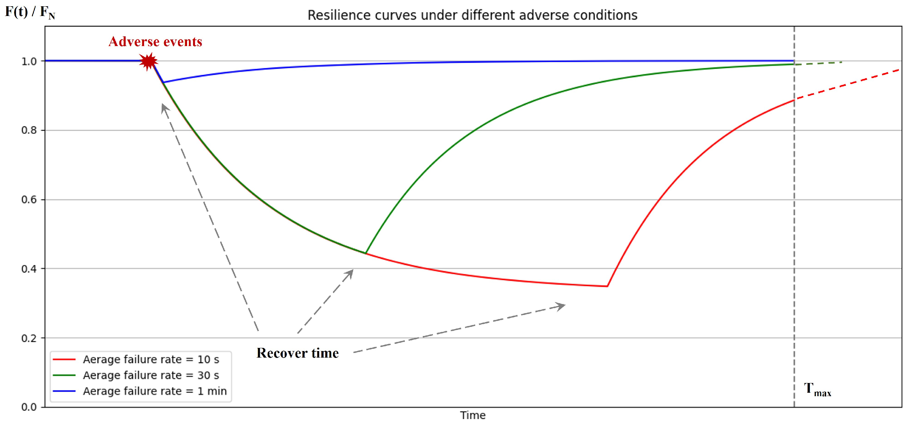
• Step 2: CTMC simulation under different conditions

Given the inherent complexity of real-world conditions, obtaining precise values for the aforementioned parameters remains a challenging task. To address this, CTMC simulations are performed under multiple threat environments and parameter configurations. For each setting, the steady-state probabilities of all system states are computed, capturing the likelihood of the system being in normal, failed, degraded, or recovering conditions when subjected to various cyber-induced disruptions. These probabilities offer a probabilistic characterization of long-term system behavior for downstream analysis.

The CTMC modeling process relies on input parameters estimated through fault injection testing or expert judgment; we conducted a sensitivity analysis to support informed design decisions. In this analysis, each key parameter—failure rate ($\lambda$), recovery rate ($\mu$), and anomaly consistency ($\sigma$)—was systematically varied within a reasonable range around its baseline value, while other parameters were held constant. This allowed us to assess how variations in these inputs affect the steady-state probabilities of CTMC states, thereby influencing resilience performance. As illustrated in Figure 8, the X-axis represents the intensity of adverse conditions, and the Y-axis denotes CTMC-based evaluation metrics such as AP and ABP. Different curves correspond to different parameter values used in the sensitivity test.

The results show that the model is particularly sensitive to changes in $\mu$, as the recovery rate directly affects both the duration and severity of performance degradation. An increase in $\mu$ leads to a marked improvement in system availability under identical threat conditions. By contrast, $\sigma$ has a relatively minor impact on AP in highly heterogeneous systems but significantly influences ABP. This reflects that anomaly consistency in such systems primarily affects the voting logic of redundant modules.

Overall, these findings highlight the practical importance of robust parameter estimation techniques and suggest that simulations should be conducted under diverse threat scenarios and parameter configurations whenever possible during this step.

• Step 3: Standardization of model coupling parameters

In this step, the normalized coupling parameters $A_i$ and $R_i$ are derived for different CTMC states based on the transition probabilities and system semantics defined in the previous stage. These parameters are rescaled to lie within interpretable ranges, allowing for seamless integration into the continuous-time performance model introduced earlier. This facilitates the transition from an abstract stochastic model to dynamic performance simulation, thereby bridging the gap between cyber-layer behavior and physical-layer impact.

The parameter values $A_i$ and $R_i$ may be either empirically derived or set via domain-specific assumptions. When needed, these values can be normalized with respect to their expected nominal values to maintain consistency across systems. Once the full set of parameters is assigned, the integrated performance function $F\left(t\right)$ can be constructed as a piecewise solution over each time segment $\Delta t_i$, governed by the corresponding degradation/recovery dynamics.

• Step 4: Resilience curve display

Finally, using the normalized parameters derived in Step 3, this step simulates the time-domain performance evolution of the CPS under adverse conditions. The output is a set of resilience curves that provide an intuitive basis for comparing the system’s robustness, rapidity, and adaptability.

Such a framework enables simulation and quantitative comparison of different defense strategies, recovery mechanisms, or architectural designs by adjusting the Markov model parameters and observing their influence on the physical domain dynamics. The shape of the curve captures both the stealthiness of certain threats and the effectiveness of recovery mechanisms. This provides a view of how cyber events in the control plane translate to physical performance impact over time. In Section 4, a case study in an ICS is presented to further illustrate the core workflow of the proposed quantitative framework.

3.4.3. Comparison with Existing Frameworks

To contextualize the advantages of the proposed framework, it is important to compare it with existing cyber resilience assessment approaches. While numerous frameworks have been developed in recent years, most fall into one of the four categories discussed in Section 2: static assessment metrics, dynamic performance modeling, cyber domain security modeling, and red-teaming or adversarial simulations. Each offers valuable perspectives but also presents limitations when applied to complex, multi-domain CPS environments. This section provides a comparative analysis between our framework and representative methods from each category, focusing on key features.

As summarized in

Table 2. Comparison between the proposed resilience assessment framework and representative existing methods across key evaluation dimensions, where ✓ indicates full support, △ indicates partial support, and × indicates limited support.

Evaluation Dimension	Static Assessment Metrics	Red-Teaming and Adversarial Simulation	Dynamic Performance Modeling	Cyber-Layer Security Modeling	Proposed Framework
Integrity	✓	△	×	△	✓
Availability	×	✓	△	✓	✓
Performance Curve	×	×	✓	×	✓
Cyber–Physical Coupling	△	△	△	×	✓
Feedback for Design	△	×	×	△	✓
Modeling Scalability	×	×	△	✓	✓

, the comparison covers six key evaluation dimensions: integrity, availability, performance curve generation, cyber–physical coupling, feedback support for design, and modeling scalability. Each method is assessed based on whether it fully supports (✓), partially supports (△), or does not support (×) the corresponding dimension. These dimensions are chosen to reflect the core capabilities required for CPS resilience assessment frameworks, encompassing both cyber and physical layers, dynamic performance representation, and the framework’s ability to support iterative design improvement and generalizability across use cases.

The results indicate that while static assessment metrics and red-teaming simulations are effective for evaluating cyber-layer attributes such as integrity and availability, they lack dynamic performance modeling and cyber–physical integration capabilities. Similarly, existing dynamic modeling approaches often capture time-dependent behavior but remain limited to specific domains or lack feedback mechanisms for system-level design optimization. The proposed framework addresses these limitations by integrating stochastic modeling of cyber-layer disruptions with physical-layer performance dynamics, thereby enabling end-to-end resilience evaluation. In addition, the framework supports design feedback and allows for flexible parameterization to improve modeling scalability across diverse application scenarios. This comparative analysis demonstrates the comprehensive nature and practical utility of the proposed approach in advancing CPS resilience engineering.

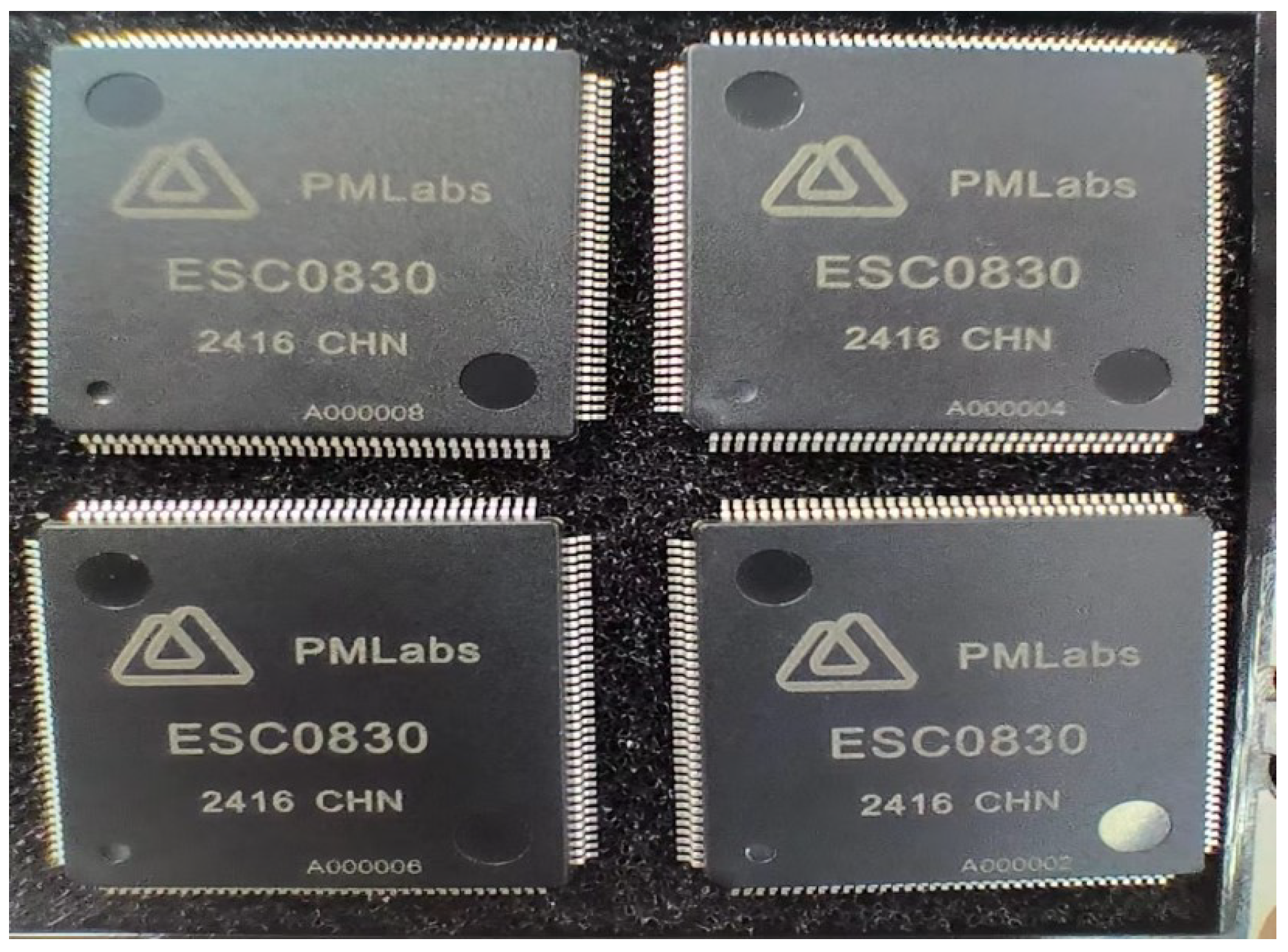
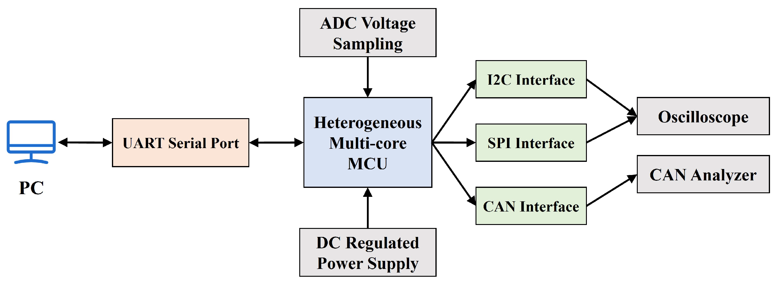
4. Case Study of Industrial Control Systems

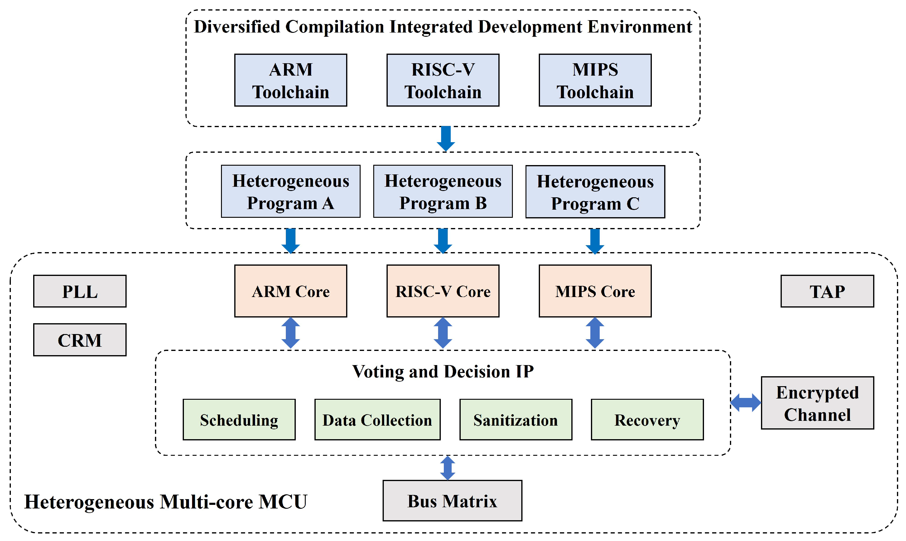
4.1. Application Scenarios and Security Design Implementation

Programmable Logic Controllers (PLCs) are critical components of ICSs, widely deployed in sectors such as manufacturing, energy, and critical infrastructure. In the context of CPSs, PLCs serve as essential nodes that bridge the cyber layer and the physical process layer. They receive input signals from field sensors, execute control logic in real time, and issue output commands to actuators, enabling continuous closed-loop interaction between computation and physical dynamics. Following the design principles outlined in Section 3.3 on the diversity-redundancy security architecture, this study develops a prototype PLC system referred to as the diversity-redundancy security PLC. Technically, the system is implemented using a heterogeneous multi-core microcontroller unit (MCU), which integrates both architectural and operational redundancy.

The custom-designed MCU includes three heterogeneous CPU cores, a lightweight polymorphic scheduler, a bus matrix, and various peripheral components. Unlike conventional single-core or homogeneous multi-core MCUs, this design introduces substantial differences among the three CPU cores. These differences span communication interfaces and memory architectures, interrupt handling mechanisms, and address mapping schemes. These cores are also supported by dedicated software toolchains to enable co-design between hardware and software. The heterogeneous CPU cores are based on three distinct instruction set architectures: ARM Cortex-M3, RISC-V Open-E906, and MIPS MicroAptiv UC. The MCU system architecture is illustrated in Figure 9, and a photograph of the physical device is shown in Figure 10. Under this heterogeneous architecture, the PLC system can perform security defense, malicious code cleansing, and resilient recovery, which are orchestrated through coordinated scheduling and runtime verification.

The primary design goal of this system is to enhance cyber resilience for PLCs as core components of industrial CPS infrastructure scenarios. However, designing for resilience presents several practical challenges:

• Trade-offs between performance overhead and security effectiveness in real-time control environments;
• The complexity of coordinating heterogeneous components to achieve fault tolerance and attack resistance;
• Lack of quantitative methods to evaluate how architectural diversity and redundancy translate into resilience benefits under dynamic cyber–physical conditions.

These challenges underscore the necessity of a theoretically grounded evaluation framework. Without a rigorous modeling and assessment mechanism, it is difficult to validate whether design interventions (e.g., heterogeneity and dynamic scheduling) truly improve the system’s ability to withstand and recover from cyber disturbances.

In this context, the modeling approach proposed in Section 3 provides an essential theoretical foundation. By capturing multi-state degradation, dynamic recovery, and cyber–physical interactions, this framework enables structured evaluation of PLC resilience under various threat scenarios. The following subsection illustrates how this approach is applied to the proposed PLC system to guide and verify design effectiveness.

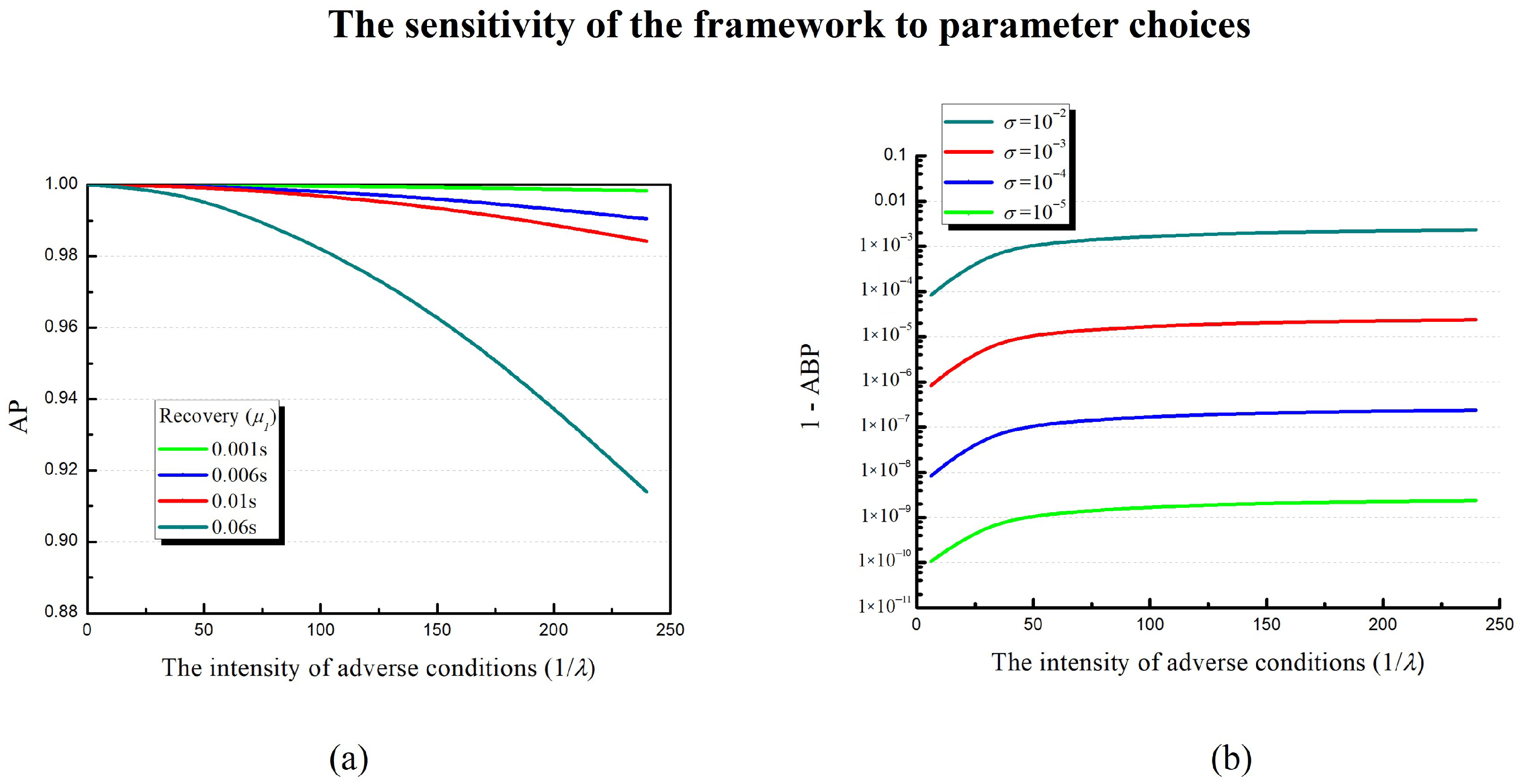
4.2. Modeling and Simulation Results

This subsection applies the CPS resilience quantitative assessment framework proposed in Section 3 to the case of the diversity-redundancy security PLC. The framework follows the four-step modeling and simulation procedure described in Section 3.4.2.

In Step 1, the key parameters to be assigned include the failure rate ($\lambda$), recovery rate ($\mu$), and malfunction consistency ($\sigma$). As shown in

Table 3. The assignment method and values of the CTMC model.

Parameters	Assignment Methods	Values
${\mu }_1$	White-box fault injection test	0.1 s
${\mu }_2$	White-box fault injection test	3 min
${\mu }_3$	White-box fault injection test	60 min
${\mu }_4$	White-box fault injection test	1 min
$\sigma$	Historical information evaluation	${10}^{-3}$

, we define these parameters based on their theoretical meanings, empirical knowledge, and penetration test results specific to the PLC under study. The parameter $\sigma$ is determined by analyzing the historical software and hardware version data as well as known shared vulnerabilities across heterogeneous components. The recovery rate $\mu$ is estimated using white-box fault injection tests, where artificial faults are introduced into redundant execution units to assess their average recovery speed. The testing methodology generally follows the process proposed in [17], and the test environment topology is shown in Figure 11. For brevity, detailed procedures are not repeated here.

According to Step 2, we define three levels of the failure rate $\lambda$ to represent high-risk, medium-risk, and low-risk operational environments. With fixed design parameters $\mu$ and $\sigma$, we perform simulations of the CTMC model under each threat scenario. The state transition probabilities and steady-state distributions are computed accordingly. The results of the simulations are summarized in

Table 4. Simulation results of CTMC model under different adverse conditions.

Adverse Conditions	Metrics	Values
λ = 10 s	AP	0.7436
	EP	0.0021
	DP	0.2543
λ = 30 s	AP	0.9189
	EP	6.09 × 10−4
	DP	0.0805
λ = 1 min	AP	0.9901
	EP	5.93 × 10−5
	DP	0.0098

, providing insight into how the PLC behaves across different environmental conditions. These results also serve as the foundation for subsequent parameter normalization and performance curve construction.

In Step 3, we standardize the key performance-influencing parameters derived from the CTMC model. This enables their integration into the coupled cyber–physical resilience model. The normalized values of critical parameters (e.g., duration of each segment and maximum response capacity) are calculated based on the outputs from Step 2 and are shown in

Table 5. The values of A and R in different resilience stages.

Resilience States	Parameters	Values
Undetectable failure	A	1
	R	0
Detectable failure	A	0.8
	R	0.1
Degraded	A	0.6
	R	0.3
Available	A	0
	R	1

. This step facilitates the transition from abstract stochastic models to dynamic performance simulations, bridging the gap between cyber-layer behavior and physical-layer impact.

Finally, leveraging the mathematical modeling framework in Section 3.2 and the parameter set established in the previous steps, we simulate and visualize the PLC’s resilience response under cyber disturbances. The resulting resilience curves are shown in Figure 12, demonstrating the time-varying performance trajectory of the system in different adverse conditions.

The resulting resilience curves reveal that, due to the relatively low failure probabilities in all three simulated conditions, the primary differences lie in the time proportions spent in degraded and available states. Typically, system resilience can be evaluated through multiple aspects, including the area under the degradation phase of the curve, recovery time, and robustness. Through the four steps outlined in this section, a comprehensive view is established, illustrating how the diversity-redundancy security architecture contributes to both resistance and recovery under adverse conditions such as cyber attacks. Note that, in certain simulation scenarios, varying parameter settings for degradation amplitude (A) and recovery rate (R) can also lead to observable differences in the resilience curves, reflecting the influence of distinct resistance and recovery strategies.

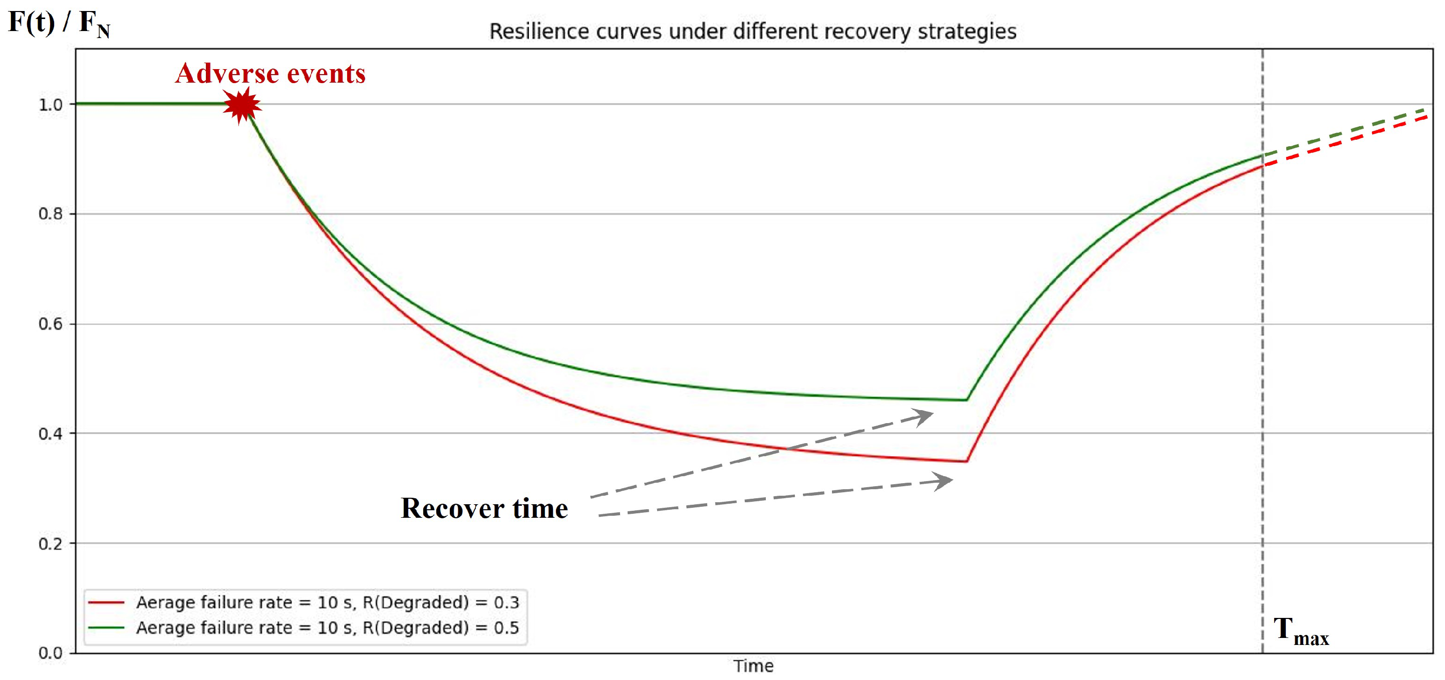
4.3. Design Optimization and Discussion

Based on the simulation results from the previous section, this part presents a targeted optimization of the PLC design, guided by the resilience assessment framework.

Given the evaluation results and practical design constraints such as latency, hardware cost, and system complexity, we prioritize enhancing the recovery rate to improve overall resilience. Thus, we propose an architectural optimization focused on context backup and rollback strategies during runtime. Specifically, the software execution process is modified to periodically save key runtime contexts and define rollback points. At these points, the state of the CPU is recorded to enable recovery in case of execution anomalies. Upon detection of a fault by the lightweight mimetic scheduler, the faulty CPU core is interrupted, and a targeted software cleansing is performed according to a predefined exception handling logic. The CPU then rolls back to its most recent saved context and re-synchronizes with the other cores before rejoining the mimetic voting process.

Figure 13 illustrates the operation of this mechanism. In the MCU, each heterogeneous core may request to update the application’s global state after computation. The scheduler collects modification requests from all three cores within a preset time window, conducts majority voting to determine the correct state, and updates the global application state accordingly. After this, a synchronization signal is broadcast to all cores, prompting them to perform a unified state reload, completing the state recovery process. This mechanism effectively shortens the downtime associated with individual core failures, improving the overall system recovery responsiveness.

To evaluate the impact of the design optimization, recovery tests were conducted on both the original and the improved PLC implementations. The results indicate that the average recovery rate increased by approximately 60%, reflecting a substantial enhancement in the system’s responsiveness to internal disruptions. Based on this updated recovery capability, the degradation-phase recovery parameter R is reset and the full resilience assessment process from Section 4.2 is repeated.

As illustrated in Figure 14, the revised resilience curves show a notable reduction in the area under the degradation phase, alongside improved system robustness and faster recovery. These improvements are particularly evident in scenarios with persistent disruptions, where the system maintained a higher performance baseline and returned to nominal operation more quickly.

It is worth noting that beyond the differences in recovery time and strategies demonstrated through the resilience curve comparisons in this section, the proposed evaluation framework and process offer considerable flexibility for customization. Key components of the framework—including the definition of resilience phases, the modeling of adverse conditions, the parameter normalization strategies, and the model formulation of the cyber layer—can be adapted to suit different system contexts and application domains. This flexibility enables the framework to be extended or tailored for a wide range of CPS configurations and resilience design needs.

In summary, the design optimization guided by the proposed resilience evaluation framework led to significant performance gains. The degradation zone was markedly reduced, system robustness improved, and overall resilience enhanced. These results validate the effectiveness of our modeling-guided feedback design approach for cyber–physical systems.

5. Conclusions

This study proposes a novel resilience evaluation framework tailored for CPSs, which establishes a quantitative method to assess system resilience under adverse disruptions. By integrating a cyber–physical Markov chain model with parameterized degradation and recovery dynamics, the framework innovatively bridges the gap between the cyber and physical layers in resilience evaluation, providing a feasible and systematic pathway for resilience-aware CPS design and analysis. To demonstrate the practical value of the proposed approach, a case study was conducted on an ICS scenario. The results confirmed that the method can support informed security design decisions, improving both the robustness and recovery capabilities of CPSs.

Future work will extend the proposed framework in two directions. First, we plan to incorporate richer threat models and probabilistic reasoning methods, such as Bayesian networks and game theory, to capture more complex cyber–physical interactions. Second, we aim to improve usability by developing supporting tools for automated parameter estimation, simulation, and resilience evaluation, enhancing the framework’s accessibility in practical CPS applications.

References

1. Almulhim, A.I. Building Urban Resilience Through Smart City Planning: A Systematic Literature Review. Smart Cities (2624-6511) 2025, 8, 22. [Google Scholar] [CrossRef]
2. Alhidaifi, S.M.; Asghar, M.R.; Ansari, I.S. A survey on cyber resilience: Key strategies, research challenges, and future directions. ACM Comput. Surv. 2024, 56, 1–48. [Google Scholar] [CrossRef]
3. Lee, H.; Kim, S.; Kim, H.K. SoK: Demystifying cyber resilience quantification in cyber-physical systems. In Proceedings of the 2022 IEEE International Conference on Cyber Security and Resilience (CSR), Rhodes, Greece, 27–29 July 2022; pp. 178–183. [Google Scholar]
4. Dibaji, S.M.; Pirani, M.; Flamholz, D.B.; Annaswamy, A.M.; Johansson, K.H.; Chakrabortty, A. A systems and control perspective of CPS security. Annu. Rev. Control 2019, 47, 394–411. [Google Scholar] [CrossRef]
5. Rus, K.; Kilar, V.; Koren, D. Resilience assessment of complex urban systems to natural disasters: A new literature review. Int. J. Disaster Risk Reduct. 2018, 31, 311–330. [Google Scholar] [CrossRef]
6. Gasser, P.; Lustenberger, P.; Cinelli, M.; Kim, W.; Spada, M.; Burgherr, P.; Hirschberg, S.; Stojadinovic, B.; Sun, T.Y. A review on resilience assessment of energy systems. Sustain. Resilient Infrastruct. 2021, 6, 273–299. [Google Scholar] [CrossRef]
7. Segovia-Ferreira, M.; Rubio-Hernan, J.; Cavalli, A.; Garcia-Alfaro, J. A survey on cyber-resilience approaches for cyber-physical systems. ACM Comput. Surv. 2024, 56, 1–37. [Google Scholar] [CrossRef]
8. Linkov, I.; Fox-Lent, C.; Read, L.; Allen, C.R.; Arnott, J.C.; Bellini, E.; Coaffee, J.; Florin, M.V.; Hatfield, K.; Hyde, I.; et al. Tiered approach to resilience assessment. Risk Anal. 2018, 38, 1772–1780. [Google Scholar] [CrossRef]
9. Koh, S.L.; Suresh, K.; Ralph, P.; Saccone, M. Quantifying organisational resilience: An integrated resource efficiency view. Int. J. Prod. Res. 2024, 62, 5737–5756. [Google Scholar] [CrossRef]
10. Ross, R.; Pillitteri, V.; Graubart, R.; Bodeau, D.; McQuaid, R. Developing Cyber-Resilient Systems: A Systems Security Engineering Approach; Technical report; National Institute of Standards and Technology: Gaithersburg, MD, USA, 2021. [Google Scholar] [CrossRef]
11. Bodeau, D.J.; Graubart, R.D.; McQuaid, R.M.; Woodill, J. Cyber Resiliency Metrics Catalog; The MITRE Corporation: Bedford, MA, USA, 2018. [Google Scholar]
12. Bodeau, D.J.; Graubart, R.D.; McQuaid, R.M.; Woodill, J. Cyber Resiliency Metrics, Measures of Effectiveness, and Scoring; The MITRE Corporation: Bedford, MA, USA, 2018. [Google Scholar]
13. Stouffer, K.; Stouffer, K.; Pease, M.; Tang, C.; Zimmerman, T.; Pillitteri, V.; Lightman, S.; Hahn, A.; Saravia, S.; Sherule, A.; et al. Guide to Operational Technology (OT) Security; Technical report; US Department of Commerce, National Institute of Standards and Technology: Gaithersburg, MD, USA, 2023. [Google Scholar]
14. White, G.B.; Sjelin, N. The NIST Cybersecurity Framework (CSF) 2.0; Technical report; National Institute of Standards and Technology: Gaithersburg, MD, USA, 2024. [Google Scholar]
15. Juma, A.H.; Arman, A.A.; Hidayat, F. Cybersecurity assessment framework: A systematic review. In Proceedings of the 2023 10th International Conference on ICT for Smart Society (ICISS), Bandung, Indonesia, 6–7 September 2023; pp. 1–6. [Google Scholar]
16. Vandezande, N. Cybersecurity in the EU: How the NIS2-directive stacks up against its predecessor. Comput. Law Secur. Rev. 2024, 52, 105890. [Google Scholar] [CrossRef]
17. Wu, J. Cyber Resilience System Engineering Empowered by Endogenous Security and Safety; Springer: Berlin/Heidelberg, Germany, 2024. [Google Scholar]
18. Abbass, H.; Bender, A.; Gaidow, S.; Whitbread, P. Computational red teaming: Past, present and future. IEEE Comput. Intell. Mag. 2011, 6, 30–42. [Google Scholar] [CrossRef]
19. Yulianto, S.; Soewito, B.; Gaol, F.L.; Kurniawan, A. Metrics and Red Teaming in Cyber Resilience and Effectiveness: A Systematic Literature Review. In Proceedings of the 2023 29th International Conference on Telecommunications (ICT), Toba, Indonesia, 8–9 November 2023; pp. 1–7. [Google Scholar]
20. Snyder, D.; Heitzenrater, C. Enhancing Cybersecurity and Cyber Resiliency of Weapon Systems: Expanded Roles Across a System’s Life Cycle; Technical report; RAND Corporation: Santa Monica, CA, USA, 2024. [Google Scholar]
21. Strom, B.E.; Applebaum, A.; Miller, D.P.; Nickels, K.C.; Pennington, A.G.; Thomas, C.B. Mitre ATT&CK: Design and Philosophy; Technical Report; The MITRE Corporation: McLean, VA, USA, 2018. [Google Scholar]
22. Xiong, T.; Lina, G.; Guifen, Z.; Donghong, Q. A intrusion detection algorithm based on improved slime mould algorithm and weighted extreme learning machine. In Proceedings of the 2021 4th International Conference on Artificial Intelligence and Big Data (ICAIBD), Chengdu, China, 28–31 May 2021; pp. 157–161. [Google Scholar]
23. Yulianto, S.; Soewito, B.; Gaol, F.L.; Kurniawan, A. Enhancing cybersecurity resilience through advanced red-teaming exercises and MITRE ATT&CK framework integration: A paradigm shift in cybersecurity assessment. Cyber Secur. Appl. 2025, 3, 100077. [Google Scholar]
24. Fink, G.A.; Griswold, R.L.; Beech, Z.W. Quantifying cyber-resilience against resource-exhaustion attacks. In Proceedings of the 2014 7th International Symposium on Resilient Control Systems (ISRCS), Denver, CO, USA, 19–21 August 2014; pp. 1–8. [Google Scholar]
25. Shin, S.; Lee, S.; Burian, S.J.; Judi, D.R.; McPherson, T. Evaluating resilience of water distribution networks to operational failures from cyber-physical attacks. J. Environ. Eng. 2020, 146, 04020003. [Google Scholar] [CrossRef]
26. Kott, A.; Linkov, I. Cyber Resilience of Systems and Networks; Springer: Berlin/Heidelberg, Germany, 2019; Volume 1. [Google Scholar]
27. Pawar, B.; Huffman, M.; Khan, F.; Wang, Q. Resilience assessment framework for fast response process systems. Process Saf. Environ. Prot. 2022, 163, 82–93. [Google Scholar] [CrossRef]
28. Clark, A.; Zonouz, S. Cyber-physical resilience: Definition and assessment metric. IEEE Trans. Smart Grid 2017, 10, 1671–1684. [Google Scholar] [CrossRef]
29. Cassottana, B.; Roomi, M.M.; Mashima, D.; Sansavini, G. Resilience analysis of cyber-physical systems: A review of models and methods. Risk Anal. 2023, 43, 2359–2379. [Google Scholar] [CrossRef]
30. AlHidaifi, S.M.; Asghar, M.R.; Ansari, I.S. Towards a cyber resilience quantification framework (CRQF) for IT infrastructure. Comput. Netw. 2024, 247, 110446. [Google Scholar] [CrossRef]
31. Cheng, Y.; Elsayed, E.A.; Huang, Z. Systems resilience assessments: A review, framework and metrics. Int. J. Prod. Res. 2022, 60, 595–622. [Google Scholar] [CrossRef]
32. Almaleh, A. Measuring resilience in smart infrastructures: A comprehensive review of metrics and methods. Appl. Sci. 2023, 13, 6452. [Google Scholar] [CrossRef]
33. Weisman, M.J.; Kott, A.; Ellis, J.E.; Murphy, B.J.; Parker, T.W.; Smith, S.; Vandekerckhove, J. Quantitative measurement of cyber resilience: Modeling and experimentation. ACM Trans. Cyber-Phys. Syst. 2025, 9, 1–25. [Google Scholar] [CrossRef]
34. Soikkeli, J.; Casale, G.; Muñoz-González, L.; Lupu, E.C. Redundancy planning for cost efficient resilience to cyber attacks. IEEE Trans. Dependable Secur. Comput. 2022, 20, 1154–1168. [Google Scholar] [CrossRef]
35. Orojloo, H.; Abdollahi Azgomi, M. Modelling and evaluation of the security of cyber-physical systems using stochastic Petri nets. IET Cyber-Phys. Syst. Theory Appl. 2019, 4, 50–57. [Google Scholar] [CrossRef]
36. Chen, C.; Wu, W.; Zhou, H.; Shen, G. A Semi-Markov Survivability Evaluation Model for Intrusion Tolerant Real-Time Database Systems. In Proceedings of the 2011 7th International Conference on Wireless Communications, Networking and Mobile Computing, Wuhan, China, 23–25 September 2011; pp. 1–4. [Google Scholar]
37. Kotenko, I.; Saenko, I.; Lauta, O. Analytical modeling and assessment of cyber resilience on the base of stochastic networks conversion. In Proceedings of the 2018 10th International Workshop on Resilient Networks Design and Modeling (RNDM), Longyearbyen, Norway, 27–29 August 2018; pp. 1–8. [Google Scholar]
38. Hausken, K.; Welburn, J.W.; Zhuang, J. A Review of Attacker–Defender Games and Cyber Security. Games 2024, 15, 28. [Google Scholar] [CrossRef]
39. Caetano, H.O.; Desuó, L.; Fogliatto, M.S.; Maciel, C.D. Resilience assessment of critical infrastructures using dynamic Bayesian networks and evidence propagation. Reliab. Eng. Syst. Saf. 2024, 241, 109691. [Google Scholar] [CrossRef]
40. Jiang, Y.; Wu, S.; Ma, R.; Liu, M.; Luo, H.; Kaynak, O. Monitoring and defense of industrial cyber-physical systems under typical attacks: From a systems and control perspective. IEEE Trans. Ind. Cyber-Phys. Syst. 2023, 1, 192–207. [Google Scholar] [CrossRef]
41. Xing, W.; Shen, J. Security Control of Cyber–Physical Systems under Cyber Attacks: A Survey. Sensors 2024, 24, 3815. [Google Scholar] [CrossRef] [PubMed]
42. Weisman, M.J.; Kott, A.; Vandekerckhove, J. Piecewise linear and stochastic models for the analysis of cyber resilience. In Proceedings of the 2023 57th Annual Conference on Information Sciences and Systems (CISS), Baltimore, MD, USA, 22–24 March 2023; pp. 1–6. [Google Scholar]
43. Garcia, M.; Bessani, A.; Gashi, I.; Neves, N.; Obelheiro, R. Analysis of operating system diversity for intrusion tolerance. Softw. Pract. Exp. 2014, 44, 735–770. [Google Scholar] [CrossRef]
44. Khan, M.; Babay, A. Making intrusion tolerance accessible: A cloud-based hybrid management approach to deploying resilient systems. In Proceedings of the 2023 42nd International Symposium on Reliable Distributed Systems (SRDS), Marrakesh, Morocco, 25–29 September 2023; pp. 254–267. [Google Scholar]
45. Shoker, A.; Rahli, V.; Decouchant, J.; Esteves-Verissimo, P. Intrusion resilience systems for modern vehicles. In Proceedings of the 2023 IEEE 97th Vehicular Technology Conference (VTC2023-Spring), Florence, Italy, 20–23 June 2023; pp. 1–7. [Google Scholar]
Figure 1. Categories of cyber resilience assessment.
Applsci 15 08285 g001
Figure 2. Proposed CPS resilience assessment framework.
Applsci 15 08285 g002
Figure 3. A typical performance resilience curve for a disrupted system. t a denotes the time at which the adverse condition occurs, t r represents the initiation of the recovery process, and t c marks the point at which the system restores to its previous condition. The time intervals between these points, along with the corresponding changes in system performance, can be used to characterize key resilience indicators such as rapidity and robustness.
Applsci 15 08285 g003
Figure 4. The curve variation of F ( t ) ) / F N under different values of A and R when the initial condition F ( t ) = F N . As t , the value of F ( t ) ) / F N will approach R / ( A + R ) .
Applsci 15 08285 g004
Figure 5. The curve variation of F ( t ) ) / F N for piecewise constant-coefficient model under different values of A and R when the initial condition F ( t ) = F N . When F ( t ) ) / F N > R i / ( A i + R i ) , system performance decreases; conversely, it increases.
Applsci 15 08285 g005
Figure 6. Schematic diagram of diversity-redundancy security architecture for enhancing the system’s ability to autonomously detect, withstand, and recover from failures or intrusions.
Applsci 15 08285 g006
Figure 7. A continuous-time Markov chain model for the proposed diversity-redundancy security architecture, consists of 13 distinct steady states.
Applsci 15 08285 g007
Figure 8. Sensitivity analysis with respect to μ and σ . (a) Sensitivity analysis of the parameter μ with respect to A P ; (b) Sensitivity analysis of the parameter σ with respect to A B P . The X-axis represents the intensity of adverse conditions ( 1 / λ , in h−1), and the Y-axis shows CTMC-based evaluation metrics (AP and ABP). Each curve corresponds to a different parameter setting used in the sensitivity analysis.
Applsci 15 08285 g008
Figure 9. Heterogeneous multi-core MCU architecture. The MCU architecture comprises 4 key subsystems: (1) heterogeneous multi-core CPU subsystem, (2) lightweight voting and decision subsystem, (3) bus and peripheral subsystem, and (4) application software and integrated development environment (IDE) subsystem.
Applsci 15 08285 g009
Figure 10. Photograph of the MCU physical device. Manufacturer: Purple Mountain Laboratories, Nanjing, China.
Applsci 15 08285 g010
Figure 11. The MCU test environment topology.
Applsci 15 08285 g011
Figure 12. PLC performance curves at λ = 10 s, 30 s, and 1 min.
Applsci 15 08285 g012
Figure 13. Context backup and cleaning recovery diagram of diverse-redundant MCU.
Applsci 15 08285 g013
Figure 14. Comparison of system resilience curves before and after improving recovery strategies.
Applsci 15 08285 g014