A Unified Machine Learning Framework for Li-Ion Battery State Estimation and Prediction ^†

Abstract

The accurate estimation and prediction of internal states in lithium-ion (Li-Ion) batteries, such as State of Charge (SoC) and Remaining Useful Life (RUL), are vital for optimizing battery performance, safety, and longevity in electric vehicles and other applications. This paper presents a unified, modular, and extensible machine learning (ML) framework designed to address the heterogeneity and complexity of battery state prediction tasks. The proposed framework supports flexible configurations across multiple dimensions, including feature engineering, model selection, and training/testing strategies. It integrates standardized data processing pipelines with a diverse set of ML models, such as a long short-term memory neural network (LSTM), a convolutional neural network (CNN), a feedforward neural network (FFNN), automated machine learning (AutoML), and classical regressors, while accommodating heterogeneous datasets. The framework’s applicability is demonstrated through five distinct use cases involving SoC estimation and RUL prediction using real-world and benchmark datasets. Experimental results highlight the framework’s adaptability, methodological transparency, and robust predictive performance across various battery chemistries, usage profiles, and degradation conditions. This work contributes to a standardized approach that facilitates the reproducibility, comparability, and practical deployment of ML-based battery analytics.

1. Introduction

As electric vehicles (EVs) become increasingly prominent in the transportation sector, the accurate prediction of lithium-ion (Li-ion) battery states has emerged as a critical component of effective and reliable energy management. Despite advances in battery technologies, the prediction of internal battery states remains a complex and unresolved challenge. This difficulty stems from the non-linear degradation behavior of Li-ion batteries and the variability introduced by diverse operational and environmental conditions [1].

The wide array of available methodologies for battery state estimation—ranging from model-based techniques to data-driven approaches—further underscores the need for a unified framework capable of managing this methodological diversity. Such a framework would support the consistent and robust estimation of various battery states, including the State of Charge (SoC), State of Health (SoH), and State of Power (SoP). It would also accommodate different preprocessing workflows and handle heterogeneous datasets, thus promoting reproducibility, scalability, and interoperability in predictive battery analytics.

Although several efforts in the literature attempt to address portions of this challenge, they are generally focused on specific aspects of battery management. For instance, the framework introduced in [2] is centered on battery reliability, emphasizing failure probability estimation and the development of early warning and fault detection strategies. In another example, Ref. [3] proposes a battery digital twin—a virtual representation of the physical battery—integrated with machine learning techniques to predict the SoC, SoH, and SoP. While both efforts contribute valuable insights, they address only selected facets of the broader state estimation problem.

In response to this gap, this paper proposes a unified framework that integrates three essential components aimed at performing battery state prediction. Battery state refers to a set of quantifiable indicators that describe the internal condition and performance characteristics of a battery at a given time. First, it introduces a battery data model that can flexibly accommodate multiple data types and sources. Second, it defines standardized data processing pipelines that ensure the consistent transformation and preparation of data for analysis. Third, it incorporates a diverse set of predictive modeling techniques, which can be selectively applied to different battery states based on data characteristics and application needs. This framework is designed for methodological flexibility and sustainability, enabling users to tailor combinations of models and processing steps to the unique demands of each predictive task. Overall, this paper presents a unified framework that emphasizes flexibility, adaptability, and sustainability, enabling users to tailor both modeling techniques and data workflows to the unique requirements of each prediction task. Its novelty relies on its capability of handling different datasets from different data sources in a structured way, different processes, and several ML models with configurable parameters aimed at predicting different battery states. All of these dimensions can be handled and monitored through this framework, providing a flexible tool to the analyst for predictive processes involving different battery states. Therefore, its technical architecture and development make it capable of being applied to diverse use cases with different requirements. So, it can be used by battery domain experts, who do not have knowledge of ML, in order to support them during battery testing procedures and cycling tests.

This article is a revised and extended version of our previous paper entitled “State of Charge Prediction of EV Li-ion Batteries with Machine Learning: A Comparative Analysis” [4], which was presented at the 13th Hellenic Artificial Intelligence Society (EETN) Conference on Artificial Intelligence (SETN 2024), held in Piraeus, Greece, between 11 and 13 September 2024. Our paper presented at the SETN conference proposed a specific pipeline for SoC estimation on one dataset. The current paper has been extended in the following directions: (i) It provides a generalized and unified framework that is capable of supporting various ML pipelines and analyses for different states of batteries. (ii) The instantiation of the proposed framework is demonstrated not only in SoC estimation but also in RUL prediction. (iii) In order to support the flexible and adaptable configuration of various ML pipelines and data processing methods, it proposes a detailed data model; and (iv) it is evaluated in various use cases, with different datasets and data requirements, thus verifying and validating its applicability and effectiveness in dealing with diverse battery testing environments.

The rest of the paper is organized as follows: Section 2 reviews the related literature. Section 3 presents the proposed unified framework for battery health state estimation and prediction with ML. Section 4 describes the instantiation of the proposed framework for SoC estimation and RUL prediction. Section 5 presents the implementation of the proposed framework and the experimental results for five different use cases. Section 6 provides a discussion on the framework and the results. Section 7 concludes the paper and outlines our plans for future work.

2. Literature Review

The automotive industry plays a vital role in the global economy and remains a central focus of technological research. With the dramatic rise in the number of vehicles, many developed countries are promoting the adoption of electric vehicles (EVs), which offer significant advantages in terms of reduced air pollution, enhanced reliability, and improved energy efficiency. Lithium-ion (Li-ion) batteries are the predominant choice for EVs due to their high energy density, lightweight components, and excellent charge/discharge cycling performance [5]. These batteries also offer a favorable balance between power and energy density, decreasing costs due to increased demand, extended lifespan, and low self-discharge rates [6,7].

Li-ion batteries come in various chemistries and configurations, each with distinct properties and performance characteristics [5]. In this context, monitoring the battery condition and accurately estimating its internal states are crucial for ensuring safe and efficient operation. The performance of a Li-ion battery directly influences an EV’s driving range, safety, and overall battery lifespan [7].

These tasks are managed by the Battery Management System (BMS), which is responsible for monitoring and estimating the battery’s states to prevent potential failures or misuse [6]. Due to the non-linear behavior of Li-ion batteries, the BMS must be highly effective to maintain safe operating conditions [8]. The core functionalities of a BMS include cell balancing, state monitoring, data acquisition, thermal regulation, and energy management [1,8]. Cell balancing mitigates voltage discrepancies among battery cells during charge/discharge cycles, while thermal management ensures that the battery operates within an optimal temperature range. Energy management guarantees the correct energy supply for each operation phase.

BMSs collect key data—such as voltage, current, and temperature—via embedded sensors [6,8]. These data are crucial not only for monitoring but also for estimating internal battery states [8]. Battery state refers to a set of quantifiable indicators that describe the internal condition and performance characteristics of a battery at a given time. In this sense, battery state estimation provides insights into the battery’s current condition through parameters like State of Charge (SoC), State of Power (SoP), State of Energy (SoE), State of Function (SoF), State of Balance (SoB), State of Temperature (SoT), State of Health (SoH), and Remaining Useful Life (RUL) [1,7]. These indicators collectively inform battery performance, remaining capacity, and degradation levels [7].

Each of these states serves a specific function:

• State of Charge (SoC) reflects the battery’s remaining capacity (Ah) and is vital for controlling charging and discharging cycles. Due to its dependence on internal chemistry, a battery’s SoC cannot be directly measured, necessitating estimation through indirect methods [8].
• State of Energy (SoE) indicates the battery’s available energy (Wh) and supports the energy management functions of the BMS. Accurate SoE estimation is essential for reliable energy delivery [8].
• State of Power (SoP) represents the battery’s capacity to deliver power (W) under specific constraints related to voltage, temperature, and SoC. SoP is crucial for safe energy transfer to the EV’s components [8].
• State of Function (SoF) evaluates the battery’s ability to deliver power under defined SoC and SoH conditions, providing insight into performance capabilities [9].
• State of Temperature (SoT) pertains to the thermal condition of the battery. Proper thermal control is imperative as excessive heat can cause degradation or even hazardous events like fire or an explosion [1].
• State of Balance (SoB) measures the uniformity of parameters such as voltage and temperature across battery cells, which is essential for optimal battery pack performance [1].
• State of Health (SoH) is defined as the ratio between the current and initial capacities of the battery. A battery reaches its End of Life (EOL) when capacity falls to 80% of its initial value, beyond which it is unsuitable for EV applications [8].
• Remaining Useful Life (RUL) estimates the remaining charge/discharge cycles before the battery reaches its EOL. This indicator is key for long-term battery usage planning and safety [8].

The aging of Li-ion batteries is driven by various mechanisms, including capacity fade, increased internal resistance, and safety deterioration caused by chemical decomposition, structural damage, and electrolyte breakdown. Factors like environmental temperature and frequent cycling accelerate these aging processes [9]. Moreover, rapid the charging and discharging of the battery and extreme environmental temperatures drastically affect the lifespan of the battery. For this reason, there is a great effort in temperature controlling and monitoring through Battery Temperature Management Systems (BTMSs) alongside ML techniques [10]. A deep understanding of these mechanisms, combined with accurate state estimation, is critical to enhancing battery longevity, improving performance, and ensuring operational safety [8,11].

Data informs decisions throughout a battery’s entire lifecycle—from speeding up material discovery and manufacturing optimization during design to predicting and classifying battery longevity for sales and deployment under varying stresses (e.g., charge/discharge rates, temperatures, and depths of discharge) [12]. Thus, the collection of adequate and appropriate variables is crucial to the analysis. As illustrated in [12], there is a large variety of public datasets regarding Li-ion batteries that demonstrate a wide range of test data and parameters. Furthermore, most of these datasets illustrate the lifetime or a certain part of the lifetime of batteries at the cell level, since they refer to experimental processes on a cell level in a laboratory environment. They depict a variety of cell chemistries, testing conditions, and procedures that evolved, reflecting the wide range of characteristics in Li-ion batteries [12]. However, at the same time, datasets describing the behavior of Li-ion batteries in real-world conditions, i.e., in the BMS of EVs, are not available due to confidentiality and ownership issues, thus making them inaccessible to the research community [13].

Although voltage, current, and temperature can be directly measured, most internal states cannot. This limitation complicates the accurate prediction of battery behavior, particularly under dynamic operating conditions and aging influences [14]. Consequently, various estimation approaches have been developed, including experimental techniques, observer- and filter-based methods, model-based methods, and data-driven approaches leveraging machine learning algorithms [8].

Figure 1 depicts a classification of the methods used in the reviewed related works per function. The first category of these methods describes the common ones for state estimation; it refers to the experimental methods that have been developed for each one of these states. The second category refers to the model-based methods, including the filter-based ones, which rely on mathematical formulas or models that describe the underlying system’s behavior. These approaches often incorporate domain knowledge and system dynamics since they contain information about the physical characteristics of the system. An example of these methods is the extended Kalman filter (EKF) method which linearizes the non-linear system of the battery. Nevertheless, the battery’s parameters are changing easily and quickly due to non-linear behavior, and hence it is necessary for this method to be combined with other model-based or data-driven methods [1]. The third category refers to the data-driven approaches, which are based on a large amount of historical data to uncover patterns and make predictions without requiring explicit knowledge of the underlying system’s dynamics. These methods, often powered by machine learning or deep learning techniques, adapt well to complex and non-linear relationships in data. An example of this category is a Transformer-based network, which only uses time-resolved battery data to predict the SoC, indicating its capability of predicting the behavior of complex multiphysics and multiscale battery systems [14]. Furthermore, a graph convolutional network (GCN) is proposed for SoH estimation, and more specifically it is applied to capture the overall degradation of the battery, while the cycles and their interconnections are depicted as a graph [15].

3. The Proposed Framework for Li-Ion Battery State Prediction

The proposed framework is designed to address the challenges of adaptability, modularity, and precision in battery health and performance prediction. The framework integrates multiple configurable components that can be tailored to different prediction problems, such as the SoC and RUL.

Figure 2 provides an overview of the framework, illustrating the data flow through its components. Its architecture is modular, enabling users to plug in different models, algorithms, and preprocessing techniques according to the datasets or applications at hand. The framework’s versatility is also underscored by its ability to accommodate diverse use cases, particularly through the integration of different datasets. Each dataset reflects distinct characteristics, such as variations in operational conditions, battery chemistry, and degradation profiles. Furthermore, this framework supports the application of datasets that describe the whole lifetime of the battery as well as datasets that describe only one cycle of the battery’s lifetime.

The proposed framework is structured around three core components that are described in the subsequent sub-sections: (i) The “Configuration for Battery State Prediction” component, where the foundational parameters, steps, and processes that govern each experimental setup are meticulously defined (Section 3.1). The “Process for Battery State Prediction” component, which encompasses the methodologies employed for data ingestion, preprocessing, and feature engineering, along with the integration of different predictive models tailored to the complexities of battery behavior (Section 3.2). The “Battery State Prediction” component, which applies and validates predictive models for battery state objectives, such as the SoC or RUL (Section 3.3).

3.1. Configuration for Battery State Prediction

The “Configuration for Battery State Prediction” component illustrates the definition of essential variables for each pipeline applied. Notably, this component facilitates the generation and application of multiple unique pipelines through diverse combinations of configurable dimensions. Thus, the configuration is achieved through a set of parameters that establish the specific characteristics of the applied pipeline. These parameters are designed to be versatile and adaptable, making them applicable across various battery states. It is also important to highlight that the configuration process enables the selection of the most suitable procedures for each pipeline in the following step, allowing flexibility in their application without necessitating the use of all available procedures. This generic approach ensures the framework’s flexibility and enables its seamless customization to address diverse analytical objectives related to different battery state predictions.

The framework includes four configurable dimensions: reference value estimation, definitions of the training and testing sets, feature selection, and ML model selection. The “Reference value estimation” dimension enables the identification of the specific state to be predicted, as well as the definition of the reference values for that state. This step is critical for ensuring a robust and accurate evaluation process. The “Definition of the training and testing set” dimension focuses on partitioning the dataset to facilitate effective model training and unbiased evaluations through the testing procedure of the ML model. The “Features selection” dimension defines a set of features to be applied to the pipeline, which are relevant to the specific battery state. Finally, the “ML model selection” dimension defines the appropriate ML model to be applied for the battery state selected.

3.2. Process for Battery State Prediction

The “Process for Battery State Estimation” component is composed of a set of seven procedures with different functionalities, meticulously designed to be executed in alignment with the predefined dimensions of the “Configuration for Battery State Prediction” component.

The procedures that constitute this component can be categorized into two broader groups: Data Management and Model Management. Data Management consists of the data ingestion, data preprocessing, and data harmonization procedures. Model Management consists of the model building, model training, model testing, and model evaluation procedures.

In Data Management, the data ingestion procedure refers to the data acquired from different sources, ensuring the integration of heterogeneous data to the pipelines. The data harmonization procedure provides the organization and unification of the data in a suitable way for subsequent analysis. The data preprocessing procedure refers to data cleaning, handling, structuring, and validating, needs that prepare the data and facilitate the upcoming analysis. It also includes feature engineering techniques for further selecting, manipulating, and transforming the raw data.

In Model Management, the model building procedure forms the basis for instrumenting and fine-tuning the algorithms that are developed. According to the former dimensions’ definition, the appropriate algorithms along with their configuration parameters are retrieved and prepared for further processing. After selecting and building the analytics model, the model training procedure performs parameter learning on the selected algorithm using the training dataset. The model testing procedure generates predictions about the battery state by employing the testing dataset. Finally, the data evaluation procedure enables the comparison of the predicted battery state with the reference value that has been defined in the configuration step. Additionally, this process enables the extraction of various evaluation metrics that reflect the performance of both the model and the overall pipeline.

3.3. Battery State Prediction

The “Battery State Prediction” component refers to the evaluation of the implemented pipeline as well as the collection and comparison of the evaluation metrics of pipelines that have been accomplished. All the above procedures are correlated with the selected battery state through the initial configuration, considering all the outlined dimensions. As mentioned before, each pipeline is characterized by a combination of dimensions, enabling the comparison of different pipelines. This comparison can be achieved either through the observation of the evaluation metrics that are assembled from each pipeline or the visualization of the predicted and reference values of the battery state regarding the implemented pipeline.

4. Instantiation of the Proposed Framework to SoC Estimation and RUL Prediction

In this Section, we describe how the components of the proposed framework, which are presented in Section 3, can be instantiated to specific use cases. In the instantiation presented herein, we consider SoC estimation and RUL prediction, since they are the most common objectives in the context of Li-Ion batteries.

4.1. Configuration of Battery State Prediction Instantiated for SoC and RUL

Figure 3 depicts the instantiation for the dimensions of the “Configuration of Battery State Prediction” component for SoC estimation and RUL prediction. This instantiation is presented in detail in the following sub-sections.

4.1.1. Reference Value Estimation

In the “Reference value estimation dimension”, the objective is either SoC or RUL. The battery state of the SoC, by definition, refers to the usable capacity of the battery in its current state in relation to the capacity in its fully charged state [16]. In general, the SoC is a non-linear feature, and its progress depends on temperature and current [17]. There are no direct ways to measure the SoC but there are many ways to obtain SoC estimations. Two well-known methods are Coulomb counting and OCV techniques; however, these methods are known for their limitations, which affect their accuracy and reliability [17]. For this reason, more robust and sophisticated methods are preferred to handle sensor errors and uncertain model knowledge [18].

We implemented three different methods to determine or estimate the reference values of the SoC:

• The “Residual to nominal capacity” method defines the SoC as the percentage of the battery’s current residual capacity compared to the nominal capacity according to the manufacturer’s specifications (see Equation (1)) [19].

$$SoC={\displaystyle \frac{C_{res}}{C_{nom}}}\times 100\%$$

(1)

• The “Current to maximum capacity” method defines the SoC as the percentage of the battery’s current capacity compared to the maximum battery’s capacity in each cycle, representing the fully charged state of the battery in each cycle (see Equation (2)) [16].

$$SoC={\displaystyle \frac{C_{curr}}{C_{max}}}\times 100\%$$

(2)

• The “Coulomb counting” method refers to the estimation of the SoC by applying the Coulomb counting algorithm, which is connected to the SoC’s previous state, the measurement of the current, the integration of that current over time, and the battery’s capacity (see Equation (3)).

$$SoC=SoC\left(t-1\right)+{\displaystyle \frac{I\left(t\right)}{Q_n}}\times \Delta t$$

(3)

We also implemented two different methods for RUL in order to predict the required amount of charge and discharge cycles from the point of the active profile to the end of the battery’s life, given the fact that the end of the battery’s life is considered to be the point that the battery’s capacity reaches 70% or 80% of its initial nominal value:

• In the “Remaining life” method, reference value of RUL is determined as the remaining battery cycles from the current cycle to the battery’s end of life.
• In the “Total life” method, the reference value is considered to be the battery’s life, and consequently the predictions of the pipeline refer to the battery’s lifetime. Thus, RUL is predicted through the subtraction of the current cycle from the predicted lifetime of the battery.

4.1.2. Definitions of the Training and Testing Sets

In this dimension, the following methods were implemented:

• The “set of datasets” assigns to the training and testing set, respectively, a different set of datasets. By leveraging separate datasets, the model’s exposure to diverse data patterns is enhanced, thus promoting a comprehensive learning process while ensuring robust testing on unseen data.
• The “set of a part of the datasets” creates the training and testing sets based on portions of multiple datasets. This method is particularly well-suited for applications where only a subset of the dataset is required, such as in the presence of pipelines with particular needs of data preprocessing or architectures. The “set of consecutives cycles” assigns to the training set a number of randomly selected consecutive cycles of the battery’s lifetime. This method is motivated by the fact that datasets associated with Li-ion batteries usually comprise charging and discharging cycles, which may either represent the entire life of the battery up to its end of life or focus on a single cycle. The testing set is defined as the subsequent cycle immediately following those used for training.
• The “set of non-consecutive cycles” creates the training set out of randomly selected non-consecutive cycles from the battery’s lifetime, and the testing set is made out of cycles that are independent.
• The “partial dataset” allocates a specified but also configurable percentage of a dataset to the training and testing sets. By allowing adjustable percentages for the training and testing sets, this method provides the flexibility to tailor the dataset split according to the specific requirements of the predictive model and the available data.

4.1.3. Features Selection

Features selection is a crucial component as it directly affects the performance, efficiency, and interpretability of the model. By identifying and utilizing the most relevant features, this process reduces the dimensionality of the dataset, thereby minimizing computational complexity and the risk of overfitting [20]. It ensures that the model focuses on the variables that have the most significant influence on the prediction task, improving both accuracy and generalizability. Moreover, feature selection enhances the interpretability of the model by simplifying its structure, making it easier to understand the relationships between input variables and predictions.

Within this framework, the following features selection procedures have been implemented, offering enhanced adjustability and flexibility to the applied pipelines:

• The “raw data” procedure considers the features as several variables that describe the behavior of the battery during cycling and can be captured as timeseries measurements from sensors connected to the batteries.
• The “statistics” procedure extracts various statistical metrics from the raw data to be used as features, such as the mean, variance, skewness, standard deviation, etc.
• The “features by resampling” procedure resamples the raw data according to a specific frequency.
• The “features by interpolation” procedure determines a mathematical function that passes through a given set of data points, which then allows for the estimation of values at points not originally included in the dataset.
• The “cycle-based features” procedure derives features from various attributes associated with either specific, configurable cycles or every cycle within the dataset, thus capturing cycle-centric characteristics.

4.1.4. ML Model Selection

Different ML algorithms are designed to handle specific types of data structures, patterns, and relationships, making the choice of the model pivotal to aligning with the unique characteristics of the dataset and the objectives of the analysis. Moreover, the complexity and interpretability of the model must also be considered, as overly complex models may lead to overfitting, while simpler models might fail to capture intricate patterns in the data.

In this implementation, we developed ML models using the following algorithms:

• Long Short-Term Memory (LSTM): LSTM is a deep learning extension of a recurrent neural network (RNN). The main advantage of RNNs is that they do not have a finite, discrete set of states to represent the system, but they are able to capture complex non-linear relationships [21]. However, RNNs usually underperform when learning long-term dependencies of time series due to the vanishing and exploding gradient problems. On the other hand, LSTM can represent non-linear dynamic systems by mapping the input to output sequences [17], and it can deal with complex conditions and degradation behaviors [22].
• Feedforward Neural Network (FFNN): An FFNN is one of the simplest types of artificial neural networks where the information moves in only one direction. Specifically, the information goes from the input layer, through the hidden layer, to the output layer, a process that corresponds to the model’s architecture. Therefore, this model has no cycles or loops in the network. Despite its simplicity, an FFNN is capable of modeling complex relations in the data and forms the basis for other more complicated neural networks [23].
• Convolutional Neural Network (CNN): CNNs belong to deep learning models and are particularly good at mapping a set of measured quantities to a desired output. These networks use filters between the layers, and as a result they benefit from the shared weights. Furthermore, they are capable of exploiting a number of historical data points in combination with the current one. Moreover, they can provide high computational speed [24].
• Automated Machine Learning (AutoML): AutoML automates the entire ML pipeline and uptakes many stages of data analysis and model development, generating a ML model ready for deployment. One of the main benefits of AutoML is that it reduces the demand for time-consuming and extensive data analyses; instead, it enables the automated building of ML applications [25]. Moreover, this method provides methods and processes to make ML available to non-ML experts, improving the efficiency of ML and accelerating research on ML. This advantage is an important reason for adding the AutoML method to the available models in this framework in order to increase the accessibility and usability of the framework even though this method is not the optimal one for several applications.
• Linear Regression (LR): It can deliver insights into the underlying physics by handling either one dimension or multiple dimensions as the input. Linear models also have a low computational cost since they can be trained offline, and online prediction requires only a single dot product after data preprocessing [26].
• Elastic Net (EN): It is a commonly used regularized LR model that combines both L1-norm and L2-norm penalties of the lasso and ridge methods, respectively [23].
• Support Vector Machine (SVM): An SVM is a supervised and nonparametric ML algorithm based on kernels. Although mainly used in classification problems, the SVM is capable of solving regression problems, which are also known as support vector regression (SVR). It addresses non-linear prediction problems that belong to a low-dimensional space by transforming them into linear ones in a high-dimensional space. The purpose of SVR is to produce an error function in which the maximum deviation of target values during training would be under a threshold and simultaneously maintain the largest possible smoothness of the function [23].

4.2. Process for Battery State Prediction Instantiated for SoC and RUL

In this section, we describe how the “Process for Battery State Prediction” component of the proposed framework was instantiated.

4.2.1. Data Ingestion

This implementation facilitates data acquisition from two primary sources: (i) the battery management system (BMS) connected with the battery of an EV and (ii) cyclers used in laboratory settings for battery testing procedures.

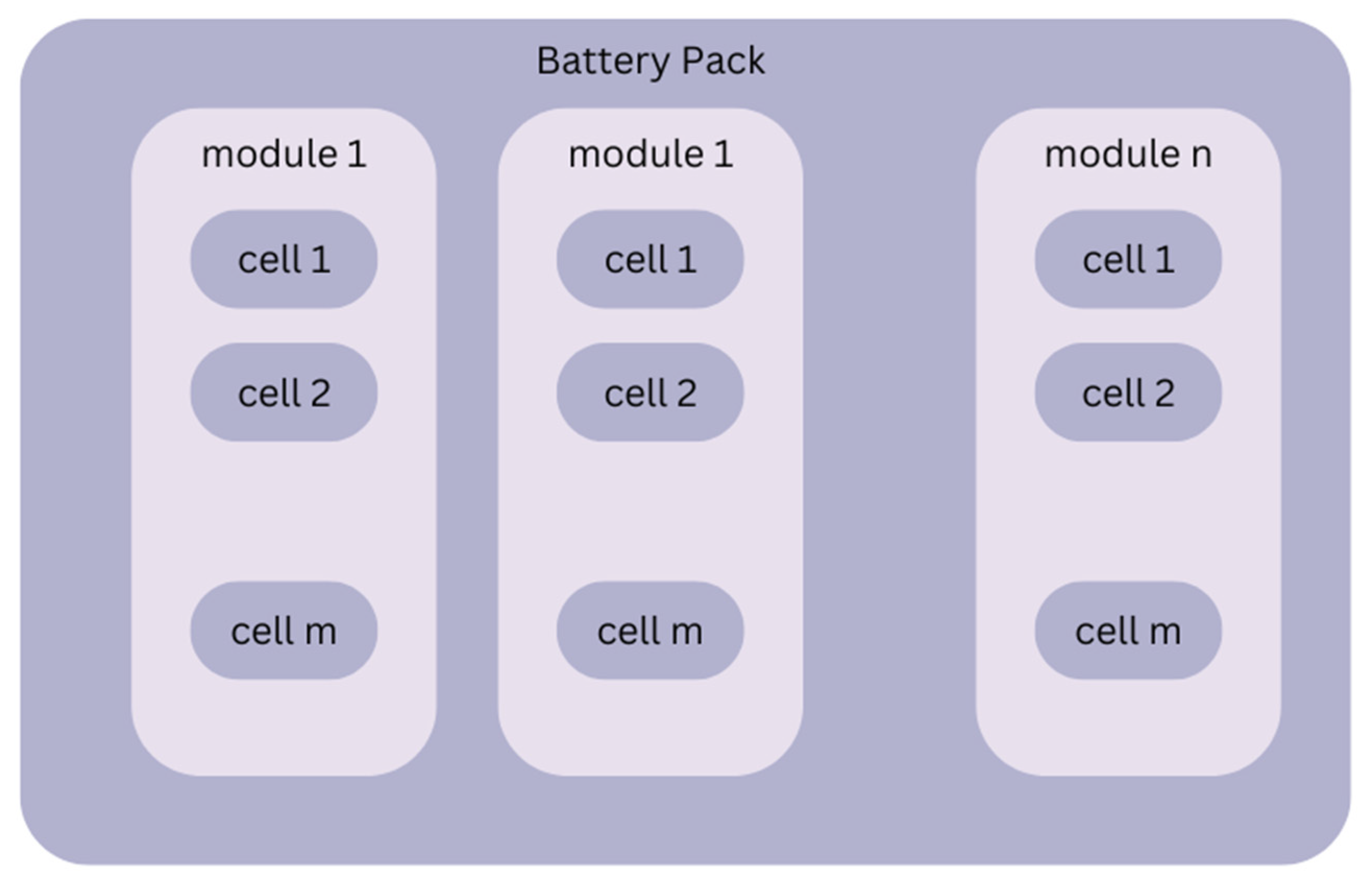
The BMS is a system located in the EV and is designed to monitor and optimize battery behavior. It is also capable of handling different cell types and chemical compositions and managing from a single module up to hundreds of them. The BMS software is designed to be accessed and updated remotely in order to provide remote maintenance functionality and to anticipate faulty situations beyond the testing phase. The BMS is a highly customized solution for monitoring, protecting, and controlling all types of batteries. It is designed to receive measurements not only from the battery pack (BP) but also from the constituent components, including the modules and cells, through sensors. Specifically, one of the main functionalities of the BMS is to measure voltage, current, and temperature, as it has restricted the capacity of the sensors that are used for measurements. EVs have a high-voltage battery pack that consists of individual modules and Li-Ion cells organized in series and parallel, as illustrating in Figure 4. A cell is the smallest, packaged form a battery can take, and a module consists of several cells connected in either series or parallel. A single cell can store and release energy. A BP is then assembled by connecting modules together in a similar way.

Multi-channel cyclers are used for cycling aging tests in labs. In each channel one cell is attached, and the cycler controls the way of charging and discharging. The cycler is wrapped from an environmental chamber in order to perform the tests in a stable environmental temperature. It can also provide measurements for voltage, current, temperature, charge and discharge capacity, energy, and power at the cell level during cycling. Some additional features that arise from these conditions are the internal resistance and inclination of the voltage curve dV/dt. Furthermore, it is able to collect metadata, including the temperature of the chamber, the charging protocol applied to the test, the cycle life of the cell, the overall operational time, the start and end times of the test, and the sampling frequency. Finally, the cell’s barcode and the number of cells that are used in the test can be considered as additional features that describe the experiment. In aging lab tests, the cells are charged and discharged periodically following a capacity threshold. The cyclers provide a controlled environment for testing by applying different C-rates (defining the charging protocol), as well as values of current and temperature [27].

4.2.2. Data Harmonization

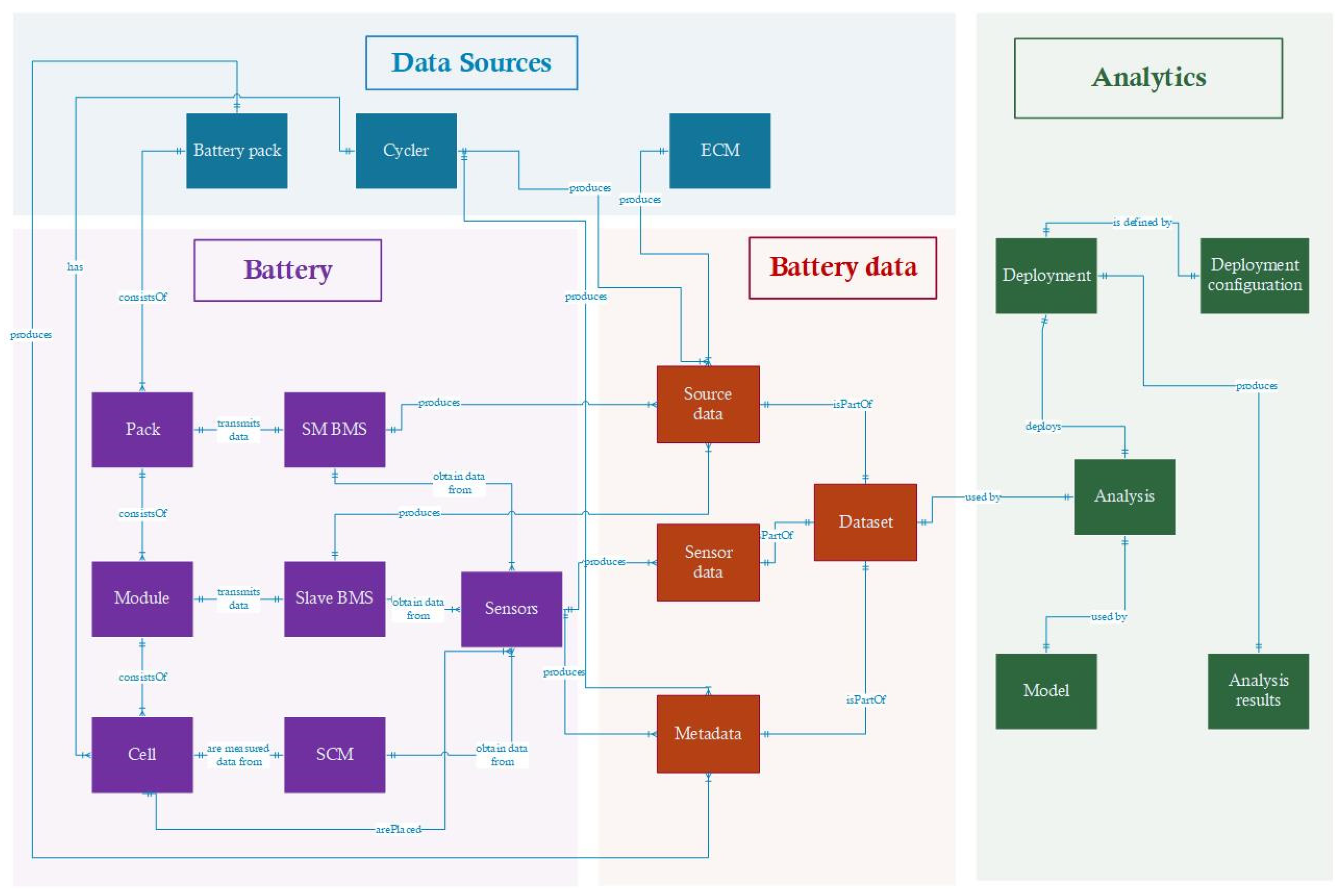
In order to enable data harmonization and data preprocessing procedures to handle the data derived from the diverse data sources, we designed and developed a related data model. A high-level view of the data model is depicted in Figure 5, while the detailed view is depicted in Figure 6. The data model demonstrates the connections as well as the relationships among the different entities. The main components of this model are the data sources, the battery, the battery data, and the analytics. Each component consists of several entities, and each entity is described by several attributes. Every entity has a unique attribute about its identity (Id) and several others that describe it.

As analyzed in the physical architecture of the battery in an EV, a BMS consists of several battery packs; a battery pack consists of several modules, and each module consists of several cells. Each of these components transmits data by a superMaster BMS, a slave BMS, and SCM, respectively. A superMaster BMS produces source data, but it also obtains data from sensors. A slave BMS produces both source and sensor data. On the contrary, only sensor data can be obtained from SCM. A cycler generates data from its sensors, source data, and metadata. All the types of data are part of a dataset that is connected to the analytics component and are used to perform data analytics with appropriate ML algorithms. Finally, a cycler has a cycler model that describes its specifications and the circumstances under which the cycling test has been performed.

4.2.3. Data Preprocessing

Data preprocessing refers to all the required data cleaning, handling, structuring, and validating needs that prepare the data and facilitate the upcoming analysis [28]. Feature construction is a procedure that focuses on the creation of new features utilizing basic, already extracted features or raw data. In this process, human intervention is necessary in order to indicate the appropriate features according to the specific domain and problem. Some common methods of feature construction is the standardization and normalization of data [19]. The input datasets are usually high-dimensional and contain many features that may be irrelevant or misleading for the selected approach of analysis. Therefore, a low-dimensional space of input data affects the model’s effectiveness and accuracy. Feature extraction helps in selecting the most relevant features properly. Among others, feature extraction can be implemented by mapping functions that distinguish the relevant features through certain metrics [25].

4.2.4. Model Building

Model building forms the basis for instrumenting and fine-tuning the selected algorithms. Based on the previously defined dimensions, the aforementioned trained algorithms and their configuration parameters are prepared for further processing. This step ensures that the chosen models are well-aligned with the problem context and data characteristics, enabling effective learning from historical patterns. It also involves initializing key settings such as learning rates, optimization strategies, and model-specific parameters to optimize performance.

Table 1. Tuning parameters and characteristics for ML models.

ML Model	Tuning Parameters	Advantages and Disadvantages
LSTM	4 layers (1st: selected neurons; 4th: activation layer ReLu) Loss: MAE Optimizer: Adam Validation split: 0.2 Epochs Batch size	+ Temporal dependencies + Handles historical data + Captures non-linear relationships − Training cost − Needs large amount of data
FFNN	4 layers with selected neurons in the 2nd and 3rd layer Activation function: ReLu Optimizer: Adam Loss: MSE Validation split: 0.2 Epochs Batch size	+ Captures non-linear relationships + Flexibility in applications + Simple architecture − No temporal dependencies − Overfitting risk
CNN	7 convolutional and max pooling layers for detailed features and scalar features, respectively 3 more layers with selected neurons in the 1st one Activation function: ReLu Optimizer: Adam	+ Local patterns detection + Less parameters than fully connected networks − Cannot handle temporal dependencies − Complex architecture
AutoML	Structured data regressor() Loss: MSE Epochs Batch size Max trials	+ Automated model selection + Automated hyperparameter tuning + High efficiency − Hard debugging − High computational cost
LR	Linear regressor()	+ Simplicity + Low data requirement − Cannot handle non-linear relationships − Cannot handle outliers
EN	Elastic Net() Grid search	+ Handles correlated features + Balances sparsity − Requires tuning of two regularization weights − Cannot handle non-linear relationships
SVR	SVR() C feature Kernel feature	+ Ignores small errors + Handles complex relationships − High training cost on large datasets − Sensitive to hyperparameter tuning

presents the architecture of each ML model applied in this framework as well as the necessary tuning parameters. There are some parameters that are demonstrated without their values since they are configurable and are defined in the configuration process of this framework. In this way the framework provides flexibility and applicability to a range of different pipelines. Moreover, in Table 1, several advantages and disadvantages that contributed to ML model selection for this application are presented for each ML model.

4.2.5. Model Training and Model Testing

Model training refers to learning the parameters of the selected algorithm by employing a subset of the selected data, i.e., the training dataset, while model testing refers to predicting either the SoC or the RUL on a different subset of the selected data, i.e., the testing dataset. The model training component involves feeding the prepared data into the selected algorithm to learn patterns, relationships, and behaviors relevant to the prediction task.

4.2.6. Model Evaluation

The metrics used for evaluation include the following: mean square error (MSE), root mean square error (RMSE), mean absolute error (MAE), mean absolute percentage error (MAPE), and R².

4.3. Battery State Prediction Instantiated for SoC and RUL

All the above procedures are correlated with the selected battery state through the initial configuration, considering all the outlined dimensions. This component enables either the observation of the performance of the applied pipelines by several evaluation metrics or the visualization of the actual and predicted values of the predicted state.

5. Implementation and Experimental Results

In this section, we present the pipelines applied with the implementation of the proposed framework. As mentioned, the framework deals with SoC estimation and RUL prediction with different attributes and configurable dimensions. We separated the experiments into five different use cases, each one addressing a different objective (i.e., either SoC estimation or RUL prediction) and being applied to different cycle aging datasets derived from tests in a controlled environment, i.e., a battery test lab (i.e., either representing the battery’s condition until its end of life or involving one cycle from its lifetime, specifically the discharge phase of a battery’s cycle) with different characteristics such as the charging protocol or the battery’s chemistry. The characteristics of each dataset applied are described in each use case below.

5.1. Technical Implementation

The implementation of these pipelines was based on the technical architecture of the proposed framework, which is depicted in Figure 7. This approach has been implemented as a standalone application that is containerized with Docker and Docker Compose to include the required services and facilitate the component’s deployment. To further decouple development and deployment from production deployment, we have considered two Docker deployment configurations. In order to make it possible for the Flask application to be deployed in production, the production deployment configuration relies on the Gunicorn “Green Unicorn”, a Python (version 3.12) Web Server Gateway Interface (WSGI) HTTP server, which allows for a quick, lightweight, and simple implementation that supports numerous workers. Additionally, data storage for the proposed implementation is based on MongoDB, the Mongoengine library, and pymongo. The core component service and the mongoDB service are both configurable (i.e., database credentials and connection details) via environmental variables in the Docker Compose setup.

As mentioned in a previous section, the “Data Management” component of the framework contains several processes regarding the “Data Ingestion”, “Data Harmonization”, and “Data Preprocessing” components. The first one can be applied through the broker accommodated to this framework or through the proposed data storage method based on the MongoDB library. Regarding the remaining components, several python libraries were employed to this application such as pandas and numpy for data preparation, manipulation, and processing as well as for the definition of huge, multi-dimensional arrays and matrices and high-level mathematical functions to work on these arrays. For the “Model Management” component of the proposed framework, several models and algorithms were implemented to achieve the prediction of the selected battery state through the process discussed in the previous section. They have been implemented as Python classes through Python packages such as Scikit-learn (or sklearn), tensorflow, and keras.

Moreover, the deployment’s results are communicated to the client applications, which are connected to the “Battery State Prediction” component, through the main interface. The suggested implementation’s main interface is a GraphQL API, which is responsible for communicating analytics data and outcomes to client applications. GraphQL is an open-source API query and manipulation language. It includes a type system, a query language and execution semantics, static validation, and type introspection, as well as the ability to read, write (mutate), and subscribe to data changes. It supports a variety of languages, including Python. API development was performed utilizing the Graphene library and the Flask-GraphQL flask-related library.

Finally, it is important to mention that this application does not examine the edge devices of the BMS such as the sensors that are connected to the battery cells, but it does examine the deployment of the proposed framework; thus all the required processes for this task took place in a virtual machine accommodated in the cloud. More specifically, this machine had the power of four CPUs with an architecture of x84_64, and the available memory was about 16 GB, while the storage capacity was about 120 GB. Furthermore, the network’s performance was up to 5 Gbit/s. Using the capabilities of this machine, the training time of the ML models for battery state prediction was in the range of 1 min to 15 h depending on the ML model applied. Specifically, the 1 min training time refers to the LR and SVR models since the 15 h training time refers to the AutoML method; this method searches for the best model for this specific application and needs multiple iterations.

5.2. Descriptions of the Features and ML Models for the Applied Use Cases

For the implemented pipelines, several features have been selected as more appropriate for these battery states according to the literature. In [16], raw data such as voltage, current, and temperature have been referred to as more suitable features as input to a neural network for SoC prediction, while voltage, current, and capacity are preferred for a model based on a support vector machine algorithm. In [26], cycle-based features are provided as input to a linear model for RUL selection, since they are domain-specific features that maintain high interpretability. Moreover, Ref. [29] presented a pipeline for SoC prediction with a deep learning model that has raw data and statistical features as the input. In summary, this pipeline has been used as the input for raw data such as voltage and temperature and statistics features such as the mean voltage and the mean current, since the latter are better values to feed the network compared to a large number of consecutive values for voltage and current.

Table 2. Features description for each group of features for the applied use cases.

Group of Features	Features
Raw data	voltage (V) current (I) temperature (T) capacity (C)
Statistics	mean voltage (Vmean) mean current (Imean)
Features by resampling	resampled voltage in 5 mHz (V5mHz) resampled voltage in 0.5 mHz (V0.5mHz) resampled current in 5 mHz (I5mHz) resampled current in 0.5 mHz (I0.5mHz)
Features by interpolation	linearly interpolated discharge capacity (QDLin) linearly interpolated temperature (TDLin)
Cycle-based features	variance ΔQ100–10 minimum ΔQ100–10 skewness ΔQ100–10 kurtosis ΔQ100–10 difference between max discharge capacity and cycle 2 slope of the linear fit to the capacity fade curve, cycles 2 to 100 intercept of the linear fit to the capacity fade curve, cycles 2 to 100 discharge capacity, cycle 2 average charge time, first 5 cycles integral of temperature over time, cycles 2 to 100 minimum internal resistance, difference between cycle 100 and cycle 2 current cycle number total discharge time internal resistance (IR)

presents the selected features for each group, as described in Section 4.1.3 regarding “Feature Selection”, which were the most suitable for SoC and RUL prediction, chosen based on the specific pipelines applied according to the literature. Correspondingly,

Table 3. Tuning parameters for ML models applied for the implementation of these use cases.

ML Model	Tuning Parameters
LSTM	4 layers (1st: 300 neurons; 4th: activation layer ReLu) Loss: MAE Optimizer: Adam Validation split: 0.2 Epochs: 100 Batch size: 150
FFNN	4 layers with 21 and 19 neurons in the 2nd and 3rd layer Activation function: ReLu Optimizer: Adam Loss: MSE Validation split: 0.2 Epochs: 100 Batch size: 150
CNN	7 convolutional and max pooling layers for detailed features and scalar features, respectively, and 3 more layers with 128 neurons in the 1st one Activation function: ReLu Optimizer: Adam
AutoML	Structured data regressor() Loss: MSE Epochs: 100 Batch size: 150 Max trials: 10
LR	Linear regressor()
EN	Elastic Net() Grid search with L1 ratio: [0.01, 0.25, 0.5, 0.75, 1]
SVR	SVR() C feature: 1 Kernel feature: ‘rbf’

demonstrates the specific parameters of each ML model applied in all use cases in this implementation, selected based on their suitability for SoC and RUL prediction.

5.3. Use Case 1: SoC Estimation on the One-Cycle Dataset

This use case deals with SoC estimation by processing the Madison dataset of McMaster University [19], which describes only one cycle of the battery’s lifetime by simulating a drive cycle of an EV. It was derived from Panasonic 18650 PF cells with NCA chemistry and a nominal capacity of 2.9 Ah. This dataset consists of 50 datasets by applying 10 different drive cycles at five different temperatures. These drive cycles were created from different charging profiles and different features such as the mean, RMS, and peak power values for each temperature that can effectively simulate different vehicle driving behaviors. Therefore, there is no knowledge of the battery’s previous condition.

For this implementation, raw data and features obtained by resampling have been selected as features. The raw data are recorded through sensors during the cycling process, while features obtained by resampling include data that are resampled at a specific and configurable frequency.

Table 4. Features applied in use case 1.

Features Selection for Use Case 1
Raw Data	Features by Resampling
voltage (V)	resampled voltage in 5 mHz (V5mHz)
current (I)	resampled voltage in 0.5 mHz (V0.5mHz)
temperature (T)	resampled current in 5 mHz (I5mHz)
	resampled current in 0.5 mHz (I0.5mHz)

presents the features that have been applied to this use case. The most suitable evaluation metric for this use case is the RMSE, which indicates the deviation of the predicted SoC from the reference value of the SoC. This metric is measured in percentage (%) since it is expressed in the same unit as the target variable, in this case the SoC.

In this use case, four different pipelines have been implemented. The details about the configuration and evaluation of these pipelines are presented in

Table 5. The configuration and evaluation of the pipelines applied in use case 1.

Pipeline	Reference Value Estimation	Definition of Training and Testing Set	Features Selection	ML Model Selection	RMSE (%)
1	residual to nominal capacity method	set of datasets ⮚ training: 8 ⮚ testing: 2	raw data ⮚ V, I, T	LSTM	1.29
2	Coulomb counting method	partial dataset ⮚ training: 70% ⮚ testing: 30%	raw data ⮚ T features by resampling: ⮚ V5mHz, V0.5mHz, I5mHz, I0.5mHz	FFNN	7.57
3	residual to nominal capacity method	partial dataset ⮚ training: 80% ⮚ testing: 20%	raw data ⮚ V, I, T	LR	5.92
4	residual to nominal capacity method	partial dataset ⮚ training: 80% ⮚ testing: 20%	raw data ⮚ V, I, T	SVR	10.39

. Figure 8 depicts the RMSE for each pipeline, and Figure 9 illustrates the actual and predicted values of the SoC for pipeline 2. In this pipeline, the model does not perform with high accuracy since the input dataset illustrates only one cycle of the battery’s lifetime, and hence a percentage of this is not adequate information for the model’s training.

5.4. Use Case 2: SoC Estimation on the Lifetime Dataset

This use case deals with SoC estimation by processing the Toyota dataset of the Toyota Research Institute (TRI) in partnership with MIT [30], which describes the whole lifetime of the battery. It consists of 124 datasets describing the whole lifetime of each cell until its capacity reaches 80% of its nominal capacity, thus representing the degradation of the battery’s maximum capacity until its end of life. In this dataset, the cycle lives range from 150 to 2300 cycles and includes 72 different fast-charging protocols. The ambient temperature was controlled by the experimental chamber to be stable at 30 °C. It was generated by Panasonic 18650 PF cells with Lithium Iron Phosphate (LPF) chemistry and a nominal capacity of 1.1 Ah.

For this implementation, raw data and statistics were selected as features. As was already mentioned, the raw data refer to variables that are registered through sensors placed on the battery cells. On the other hand, statistics are features referring to extracted statistical measurements from the raw data.

Table 6. Features applied in use case 2.

Features Selection for Use Case 2
Raw Data	Statistics
voltage (V)	mean voltage (Vmean)
current (I)	mean current (Imean)
temperature (T)
capacity (C)

presents the features that have been applied for this use case. In this use case, the most suitable evaluation metric is the RMSE, which indicates the deviation of the predicted SoC from the reference value of the SoC. This metric is measured in percentage (%) since it is expressed in the same unit as the target variable, in this case the SoC.

In this use case, seven different pipelines have been implemented. The details about their configuration and their evaluation are presented in

Table 7. The configuration and evaluation of the pipelines applied in use case 2.

Pipeline	Reference Value Estimation	Definition of Training and Testing Set	Features Selection	ML Model Selection	RMSE (%)
5	residual to nominal capacity method	set of datasets ⮚ training: 5 ⮚ testing: 2	raw data ⮚ V, T statistics ⮚ Vmean, Imean	LSTM	0.6
6	current to maximum capacity method	set of consecutive cycles ⮚ training: 5 ⮚ testing: 1	raw data ⮚ V, I, C, T	LSTM	0.25
7	current to maximum capacity method	set of consecutive cycles ⮚ training: 5 ⮚ testing: 1	raw data ⮚ V, I, C, T	LR	0.3
8	current to maximum capacity method	set of consecutive cycles ⮚ training: 5 ⮚ testing: 1	raw data ⮚ V, I, C, T	SVR	6.27
9	current to maximum capacity method	set of consecutive cycles ⮚ training: 5 ⮚ testing: 1	raw data ⮚ V, T statistics ⮚ Vmean, Imean	FFNN	2.85
10	current to maximum capacity method	set of consecutive cycles ⮚ training: 5 ⮚ testing: 1	raw data ⮚ V, T statistics ⮚ Vmean, Imean	autoML	2.14
11	residual to nominal capacity method	set of non-consecutive cycles ⮚ training: 9 ⮚ testing: 9	raw data ⮚ V, T, IR statistics ⮚ Vmean, Imean	autoML	2.7

. It is important to notice that the number of each pipeline is unique due to its specific configuration of the parameters. For this reason, the enumeration of each pipeline is differentiated, as illustrated in tables that describe the details of each pipeline applied. Figure 10 depicts the RMSE for each pipeline applied for SoC prediction in this use case, and Figure 11 illustrates the actual and predicted values of the SoC for pipeline 6. In this pipeline the LSTM performs with high accuracy since it can capture the battery’s behavior with the selected features and the proper amount of data through its lifetime. In summary, five randomly selected consecutive cycles through the battery’s lifetime are provided as the input dataset, increasing the flexibility and robustness of the pipeline. Moreover,

Table 8. The evaluation of pipeline 11 for RUL prediction in several cycles.

Cycle Number	RMSE (%)
75	3.24
175	2.70
275	3.09
375	3.56
475	2.82
575	3.63
675	3.71
775	4.65
875	6.33

and Figure 12 present in detail the RMSE metric as well as the specific cycle number for each one of the nine non-consecutive cycles used during the test in pipeline 11.

5.5. Use Case 3: RUL Prediction on the Lifetime Dataset

This use case deals with RUL prediction by processing the Toyota dataset, which describes the whole lifetime of the battery until its capacity reaches 80% of its nominal capacity. It should be noted that in order to perform RUL prediction, it is necessary to use a dataset that contains the whole lifetime of the battery to train the ML models, and it is to be used as the reference value of the prediction.

For this implementation, cycle-based features (i.e., features that are based on the cycle number) and features extracted by interpolation have been selected as features, which have been extracted from the first 100 cycles of each dataset.

Table 9. Features applied in use case 3 (ΔQ_100–10: the change in discharge voltage curves between cycles 100 and 10; QDLin and TDLin: linearly interpolated discharge capacity and temperature, respectively).

Features Selection for Use Case 3
Cycle-Based Features		Features by Interpolation
variance group	⮚ Variance ΔQ100–10	QDLin
discharge group	Variance ΔQ100–10 Minimum ΔQ100–10 Skewness ΔQ100–10 Kurtosis ΔQ100–10 Discharge capacity, cycle 2 Difference between max discharge capacity and cycle 2	TDLin
full group	Variance ΔQ100–10 Minimum ΔQ100–10 Slope of the linear fit to the capacity fade curve, cycles 2 to 100 Intercept of the linear fit to the capacity fade curve, cycles 2 to 100 Discharge capacity, cycle 2 Average charge time, first 5 cycles Integral of temperature over time, cycles 2 to 100 Minimum internal resistance, difference between cycle 100 and cycle 2
current cycle number
total discharge time
internal resistance (IR)

presents the features that have been applied to this use case. In this use case, the most suitable metric is accuracy, which indicates the deviation of the predicted RUL from the reference value of the RUL, and it is measured in percentage (%), while the RUL is expressed in cycles.

For this use case, seven different pipelines have been implemented. The details about the configuration and evaluation of these pipelines are presented in

Table 10. The configuration and evaluation of the pipelines applied in use case 3.

Pipeline	Reference Value Estimation	Definition of Training and Testing Set	Features Selection	ML Model Selection	Accuracy (%)
12	total life method	set of a part of the datasets ⮚ training: 100 cycles of 85 datasets ⮚ testing: 100 cycles of 25 datasets	cycle-based features ⮚ variance group	LR	80.21
13	total life method	set of a part of the datasets ⮚ training: 100 cycles of 85 datasets ⮚ testing: 100 cycles of 25 datasets	cycle-based features ⮚ discharge group	LR	84.45
14	total life method	set of a part of the datasets ⮚ training: 100 cycles of 85 datasets ⮚ testing: 100 cycles of 25 datasets	cycle-based features ⮚ full group	LR	89.09
15	total life method	set of a part of the datasets ⮚ training: 100 cycles of 85 datasets ⮚ testing: 100 cycles of 25 datasets	cycle-based features ⮚ variance group	EN	80.21
16	total life method	set of a part of the datasets ⮚ training: 100 cycles of 85 datasets ⮚ testing: 100 cycles of 25 datasets	cycle-based features ⮚ discharge group	EN	82.79
17	total life method	set of a part of the datasets ⮚ training: 100 cycles of 85 datasets ⮚ testing: 100 cycles of 25 datasets	cycle-based features ⮚ full group	EN	89.09
18	remaining life method	set of datasets ⮚ training: 85 ⮚ testing: 25	features by interpolating ⮚ QDLin, TDLin cycle-based features ⮚ current cycle, total	CNN	85.08

. Figure 13 presents the accuracy for each pipeline, and Figure 14 illustrates the actual and predicted values of the RUL for pipeline 18. This figure is a scatterplot since RUL is a number referring to the remaining cycles of each battery and thus of each dataset applied in the testing process.

5.6. Use Case 4: SoC Estimation on the Lifetime Dataset

This use case deals with SoC estimation by processing a dataset created in the context of the European Union’s Horizon 2020 project MARBEL “Manufacturing and assembly of modular and reusable EV battery for environment-friendly and lightweight mobility” that describes the whole lifetime of the battery [31]. It consists of 12 datasets describing the complete lifetime until the capacity reaches a certain percentage of its nominal capacity. This parameter has a range of values, from 91% to 99%, and thus, in some of these datasets, we can observe the degradation of the battery’s maximum capacity. They have been created from different charging profiles, enabling the investigation of how each charging protocol affects the battery’s cycle life. The cycle lives range from 400 to 500 cycles, and the datasets include four different charging protocols. The ambient temperature was controlled by the experimental chamber to be stable either at 10 °C or at 23 °C. It has been generated by CALB Prismatic Lithium-ion cells with NMC chemistry and a nominal capacity of 58 Ah.

For this implementation, raw data and statistics have been selected as features.

Table 11. Features applied in use case 4.

Features Selection for Use Case 4
Raw Data	Statistics
voltage (V)	mean voltage (Vmean)
current (I)	mean current (Imean)
temperature (T)
capacity (C)

presents the features that have been applied to this use case.

In this use case, the most suitable evaluation metric is the RMSE, and it is measured in percentage (%) since it is expressed in the same unit as the target variable, in this case the SoC. In this case, four different pipelines have been implemented. The details about their configuration and their evaluation are presented in

Table 12. The configuration and evaluation of the pipelines applied in use case 4.

Pipeline	Reference Value Estimation	Definition of Training and Testing Set	Features Selection	ML Model Selection	RMSE (%)
19	residual to nominal capacity method	partial dataset ⮚ training: 80% ⮚ testing: 20%	raw data ⮚ V, I, C, T	LR	0.09
20	residual to nominal capacity method	partial dataset ⮚ training: 80% ⮚ testing: 20%	raw data ⮚ V, I, C, T	SVR	6.41
21	residual to nominal capacity method	partial dataset ⮚ training: 80% ⮚ testing: 20%	raw data ⮚ V, T statistics ⮚ Vmean, Imean	FFNN	2.29
22	residual to nominal capacity method	partial dataset ⮚ training: 80% ⮚ testing: 20%	raw data ⮚ V, T Statistics ⮚ Vmean, Imean	autoML	5.37

. Figure 15 depicts the RMSE for each pipeline, enabling the visualization of each pipeline’s performance, and Figure 16 illustrates the actual and predicted values of the SoC for pipeline 21. In this use case, the number of datasets is limited, as described before, as well as the range of degradation of each battery. Nevertheless, pipeline 21 presents high accuracy since the features selected and the amount of training data are adequate and appropriate for this approach. Therefore, the pipelines that can be handled by this framework present diversity on data quality and quantity, enhancing the framework’s flexibility and efficiency. Finally, in this pipeline, the input dataset presents a few spikes on the battery’s behavior due to capacity imbalance in a few cycles. The model is not incapable of capturing this abnormality, since the training dataset is not adequate.

5.7. Use Case 5: SoC Estimation on the Lifetime Dataset

This use case deals with SoC estimation by processing a dataset created in the context of the aforementioned MARBEL project that describes the whole lifetime of the battery [31]. This dataset is different from the one used in Section 5.4. It consists of two datasets that describe the complete lifetime until the capacity reaches a certain percentage of its nominal capacity. This parameter for the first dataset was 95% and 98% for the second one. Thus, in the first one we can observe the degradation of the battery’s maximum capacity, while in the second one, we can observe a smaller degree of fading in this feature. These datasets have been created from different charging profiles. The cycle lives range from 700 to 883 cycles, and the datasets include two different charging protocols. The ambient temperature was controlled by the experimental chamber to be stable at 35 °C. This dataset has been generated by CALB Prismatic Lithium-ion cells with NMC chemistry and a nominal capacity of 58 Ah.

For this implementation, raw data and statistics have been selected as features.

Table 13. Features applied in use case 5.

Features Selection for Use Case 5
Raw Data	Statistics
voltage (V)	mean voltage (Vmean)
current (I)	mean current (Imean)
temperature (T)
capacity (C)

presents the features that have been applied to this use case. In this use case, the most suitable evaluation metric is the RMSE, and it is measured in percentage (%) since it is expressed in the same unit as the target variable, in this case the SoC.

In this case, four different pipelines have been implemented. The details about the configuration and evaluation of these pipelines are presented in

Table 14. The configuration and evaluation of the pipelines applied in use case 5.

Pipeline	Reference Value Estimation	Definition of Training and Testing Set	Features Selection	ML Model Selection	RMSE (%)
23	residual to nominal capacity method	partial dataset ⮚ training: 80% ⮚ testing: 20%	raw data ⮚ V, I, C, T	LR	0.07
24	residual to nominal capacity method	partial dataset ⮚ training: 80% ⮚ testing: 20%	raw data ⮚ V, I, C, T	SVR	3.32
25	residual to nominal capacity method	partial dataset ⮚ training: 80% ⮚ testing: 20%	raw data ⮚ V, T statistics ⮚ Vmean, Imean	FFNN	3.41
26	residual to nominal capacity method	partial dataset ⮚ training: 80% ⮚ testing: 20%	raw data ⮚ V, T statistics ⮚ Vmean, Imean	autoML	14.7

. Moreover, Figure 17 depicts the RMSE for each pipeline, and Figure 18 illustrates the actual and predicted values of the SoC for pipeline 25. This figure is dense since the testing dataset contains several cycles from the battery’s lifetime. In this implementation, as in use case 4, the number of datasets is restricted as well as the range of the batteries’ degradation. Nevertheless, pipeline 25 presents satisfactory accuracy in SoC prediction since the model, the features selected, and the training dataset are adequate and efficient for this application.

6. Discussion

The experimental evaluation of the proposed unified framework across diverse datasets and use cases provides significant insights into its flexibility, performance, and broader applicability. The design philosophy behind the framework—centered on configurability and modularity—has proven effective in adapting to both single-cycle and lifetime battery data, supporting a wide range of predictive objectives including State of Charge (SoC) estimation and Remaining Useful Life (RUL) prediction.

The variety of implemented pipelines underscores the impact of design choices—such as feature selection strategies, training/testing splits, and machine learning model selection—on the final predictive accuracy. For instance, LSTMs consistently performed well in timeseries-based SoC estimation, particularly when combined with raw or resampled features, reflecting their strength in capturing temporal dependencies in battery behavior. Conversely, simpler models such as linear regression and Elastic Net demonstrated competitive performance for RUL prediction tasks when applied with carefully engineered cycle-based features, indicating that model complexity does not always equate to higher accuracy, particularly when data are well-structured and features are meaningful.

For further evaluations of the proposed framework’s efficiency, the results of approaches based on the literature have been compared with the ones of pipelines applied through this framework. More specifically, we performed a comparative analysis between pipelines 1 and 14 and pipelines implemented based on the literature regarding the SoC. Pipeline 1 was compared with the pipeline that was implemented with an LSTM model for SoC prediction and analyzed in [17], in terms of methodology and performance. In

Table 15. Comparative analysis between pipeline 1 for SoC prediction through this framework and a pipeline based on the literature.

Madison Dataset
Parameters	Approach Based on Literature	Approach Based on Use Case 1, Pipeline 1
Reference value estimation	residual to nominal capacity method	residual to nominal capacity method
Training dataset	8 datasets	8 datasets
Testing dataset	2 datasets	2 datasets
Model	LSTM	LSTM
Epochs on training	250	100
Nodes on model	500	300
Features	raw data: V, I, T	raw data: V, I, T
RMSE (%)	1.67	1.29

, the configuration parameters are presented for each pipeline for a clearer and more constructive comparison. In both pipelines, SoC prediction has been used the Madison dataset [19], which has been described in use case 1.

In the case of SoC prediction, it is obvious that the differences between these two pipelines include the architecture of the model and the computational cost for the training process. Τhe RMSE metric in each pipeline shows that there is a slightly better performance of pipeline 1 in use case 1, indicating the importance of the model’s configuration. From this comparison, we can observe that the implemented framework is capable of handling different approaches for battery state prediction with the same or better performance, illustrating its flexibility and robustness in terms of pipeline configuration and behavior.

For further evaluations we performed paired t-tests between different applied pipelines with the purpose of examining whether the difference in the pipelines’ performance is statistically important or not. In the first place, we compared pipelines 8 and 9, and by the value of the p-value, we can conclude that the difference in mean squared errors is highly statistically significant. In other words, the FFNN pipeline significantly outperforms the SVR pipeline in terms of RMSE (p << 0.05). In a similar way, from the second comparison that we performed, we can observe that the autoML pipeline outperforms the FFNN model, and this difference is statistically important since a p-value of effectively zero indicates that the difference in mean squared errors is highly significant. In

Table 16. Statistical analysis between applied pipelines.

Paired t-Test
Pipelines Compared	t-Statistic	p-Value
pipeline 8: SVR model pipeline 9: FFNN model	−19.0473	4.91 × 10−60
pipeline 21: FFNN model pipeline 22: autoML model	−521.7533	<<0.0001

, the values of the parameters of paired t-tests are presented for each comparison conducted.

Moreover, the framework’s ability to accommodate data from various sources—ranging from EV battery management systems to laboratory cyclers—highlights its practical utility in both research and industrial environments. This versatility is further enhanced by its support for different levels of data granularity and preprocessing workflows, making it suitable for both real-time applications and long-term degradation analysis.

Importantly, the framework contributes to the battery analytics field by offering a standardized methodology for comparative model evaluations. This is particularly relevant given the heterogeneous and fragmented nature of current research efforts, where diverse datasets and ad hoc pipelines often hinder reproducibility and comparability. By decoupling the configuration, processing, and prediction components, the framework enables systematic experimentation and benchmarking, promoting methodological transparency and scalability.

Finally, while some ML models like AutoML introduced automation benefits, their performance varied depending on dataset characteristics, reinforcing the need for careful pipeline designs. These observations not only validate the framework’s configurability but also offer practical guidelines for tailoring pipelines to specific use cases.

7. Conclusions and Future Work

This work presented a unified, modular, and extensible framework for Li-ion battery health state estimation and prediction, leveraging machine learning methodologies. The proposed framework integrates flexible configuration parameters, standardized data processing pipelines, and a wide selection of predictive modeling techniques to address the diverse and complex requirements of battery state prediction tasks. By instantiating this framework for both SoC estimation and RUL prediction, we demonstrated its versatility and practical applicability across a variety of datasets and experimental conditions.

Through a series of comprehensive use cases—including single-cycle and lifetime battery datasets—we validated the framework’s adaptability across different configurations. The results confirmed that the choice of pipeline components, including feature engineering techniques and ML algorithms, significantly influences predictive performance. In particular, methods such as the LSTM and linear regression showed strong results in appropriate contexts, while AutoML proved to be a viable option for automating model selection and tuning, albeit with variable outcomes depending on dataset characteristics.

The main contribution of this work lies in offering a systematic approach that promotes the reusability, transparency, and comparability of battery state estimation models. This unified methodology addresses many of the current challenges in battery analytics, such as heterogeneous data integration, state-dependent model selection, and the need for standardized evaluation protocols.

Our future work will move towards the following directions: First, we will investigate the instantiation of the proposed framework to additional battery state objectives, such as SoH, SoP, and SoE. Second, we will integrate hybrid approaches that combine ML with physics-based modeling to enhance interpretability and robustness. In this way, we can evaluate various degradation mechanisms and battery chemistries regarding their influence in the pipeline’s effectiveness and adjustability. Third, we will use datasets with information and variables from a BMS that depicts real-world driving conditions with the purpose of demonstrating the framework’s robustness and flexibility under dynamic operating conditions. Moreover, we will study the influence of the battery’s chemistry and temperature in the effectiveness of the pipelines regarding several battery states. This would be achieved by applying extensive pipelines on datasets with different battery chemistries and in different ambient temperatures and by applying the method of transfer learning between pipelines that use datasets referring to batteries with different cell chemistries and temperatures. Finally, we will apply the framework to real-time applications, and we will deploy it on edge computing platforms in order to facilitate its use in commercial BMSs.