Article

Modeling of Dry Clutch Wear for a Wide Range of Operating Parameters

1
Faculty of Mechanical Engineering and Naval Architecture, University of Zagreb, Ivana Lučića 5, 10002 Zagreb, Croatia
2
Ford-Werke GmbH, 50769 Cologne, Germany
*
Author to whom correspondence should be addressed.
Appl. Sci. 2025, 15(15), 8150; https://doi.org/10.3390/app15158150
Submission received: 17 June 2025 / Revised: 15 July 2025 / Accepted: 17 July 2025 / Published: 22 July 2025
(This article belongs to the Section Mechanical Engineering)

Abstract

The paper presents an experimentally validated regression model for dry clutch friction lining wear, accounting for the influence of clutch temperature, initial slip speed, torque, and closing time. The experimental data have been collected by using a custom-designed disk-on-disk computer-controlled tribometer and conducting repetitive real operation-like clutch closing cycles for different levels of the above operating parameters. The model is designed to be cycle-wise, predicting cumulative worn volume expectation and standard deviation after each closing cycle. It is organized around three distinctive submodels, which provide predictions of: (i) wear rate expectation, (ii) wear rate variance, and (iii) elevated wear rate during run-in operation. Finally, the wear rate expectation and variance submodels and the overall, cumulative worn volume model are validated on independent experimental datasets. The main novelty of the presented research lies in the development of stochastic multi-input cycle-wise dry cutch wear model for clutch design and monitoring applications.

1. Introduction

Owing to their low cost and high operational efficiency, dry friction clutch systems have been widely used in automotive manual transmissions, but also in Automated Manual Transmissions (AMT) [1], Dual Clutch Transmissions (DCT) [1,2], continuously variable transmission (CVT) [3] and electric systems [4]. On the other hand, in the absence of active cooling of friction surfaces in dry clutches, they experience intense temperature variations, affecting the clutch friction lining wear [5] and clutch torque controllability [6].
The literature mostly deals with experimental analyses of wet clutch wear. Several wear mechanisms are identified in [7] for copper-based friction material in wet conditions, which are micro-plowing, plastic deformation, abrasive wear and delamination wear. In the first stage of clutch life for paper-based friction materials, the friction contact temperature is found to have dominant influence on clutch wear, while later in the clutch life mechanical parameters also become influential [8]. As different friction contact areas can experience different temperatures, the temperature distribution along the friction surface is analyzed in [9], both numerically and experimentally using a pin-on-disk tribometer. On the other hand, investigations made for organic friction materials for dry clutches are often focused on influence of individual component in composite material like silicon carbide and graphite fillers [10], different resin types [11] or possibility of replacing unsustainable fibers with rattan fibers [12]. Several wear mechanisms are also analyzed for dry friction clutches, including adhesive wear [13], oxidative wear and abrasive wear [14]. Influence of normal force and slip speed is investigated and described using a wear mechanism map in [15]. During regimes of low and mild slip speeds and pressures the tribofilm on the friction surface is naturally formed which helps to stabilize coefficient of friction and control wear [16]. During aggressive usage patterns in real-world operation rapid wear was observed in [17]. Influence of different groove patterns on clutch life is investigated in [18]. Distribution of contact pressure and wear over the friction lining surface is described in [19]. A physical model of steel-on-steel adhesive wear mechanism is developed in [13], where the processes of line sliding, accumulation and transfer of material are analyzed. A data-driven model is proposed in [20] to describe the wet clutch wear behavior depending on the number of clutch engagements. The investigation of wear processes in automotive industry is often focused on braking system. Recent research has demonstrated the potential of pyroelectric materials for detection and prediction of brake pads wear [21]. These materials also possess the ability to generate electric energy for low-power sensor supply [22]. Similar materials to those used in clutch linings are used for braking system, and it has been shown that the wear rate is strongly dependent on temperature, pressure and sliding speed [23].
This paper deals with experimental characterization and data-driven modeling of organic friction material abrasive wear for dry clutches. The core of the proposed wear model corresponds to a wear rate regression submodel with four inputs corresponding to single clutch closing cycle features: average clutch interface temperature, initial slip speed, average clutch torque, and closing time. The experimental data used for wear rate model parameterization have been collected by using a custom-designed disk-on-disk tribometer and real clutch friction materials to make the wear conditions realistic [24]. The predicted wear rate is multiplied with the dissipated friction energy to calculate the incremental worn volume, which is then integrated to predict the cumulative worn volume. As a wear process is a subject of variability, the wear expectation model is accompanied with a variability model aimed to provide worn volume variance and related 95% confidence interval (CI). The increased wear rate during the clutch run-in (RI) phase, i.e., at the beginning of clutch life, is accounted for by scaling the wear rate by a run-in weighting function derived from the experimental data and fed by the cumulative dissipated energy. The overall wear model is experimentally validated on separate experimental datasets collected for steady-state and transient conditions.
The main contributions of the paper include: (i) experimental characterization of dry clutch wear rate for a wide set and range of operating parameters, (ii) developing a multi-input wear rate regression model, and (iii) proposing a cumulative wear model accounting for run-in effect and wear variability.
The remaining part of the paper is organized as follows. Section 2 describes the disk-on-disk tribometer including its control system. Section 3 deals with design of wear characterization and validation experiments. The characterization results themselves are presented and analyzed in Section 4. Section 5 outlines the structure of overall wear model and presents its run-in submodel. Section 6 and Section 7 deal with wear rate expectation and variability submodels, respectively. Validation and analysis of the overall wear rate model are presented in Section 8. Concluding remarks are drawn in Section 9.

2. Materials and Methods

2.1. Mechanical Subsystem

The active part of disk-on-disk tribometer (Figure 1; [24,25]) consists of rotational and vertical servo-axes. The rotational axis carries the original dry clutch friction plate (Figure 1d), and it is placed on a rotating table powered directly by an electric servomotor and cooled by water supplied via a dynamic seal-based coupling. The vertical axis consists of the following elements given in bottom-up order: (i) pressure plate cut from the clutch flywheel and equipped with a temperature sensor positioned at 4 mm axial distance from the friction contact surface, (ii) water-cooled disk, (iii) custom-designed leaf spring suspension that mitigates the non-parallelism between the friction and pressure plate and related occurrence of hot spots, (iv) a set of three three-axial piezoelectric force sensors providing measurement of clutch normal force and torque, and (v) an electric servomotor and a spindle acting as a source of normal force.
A set of linear guides is used to provide stiff mechanical support for the entire vertical axis. They are positioned between the force sensors and the source of normal force (green bell in Figure 1a) to avoid any parasitic transfer of forces from the pressure plate to the surrounding, thus facilitating high precision of normal force/torque measurement system. It should be noted that only one side of friction plate is in sliding contact with the pressure plate, so that the measured torque is a half of that occurring in the real clutch for the same normal force.

2.2. Control Subsystem

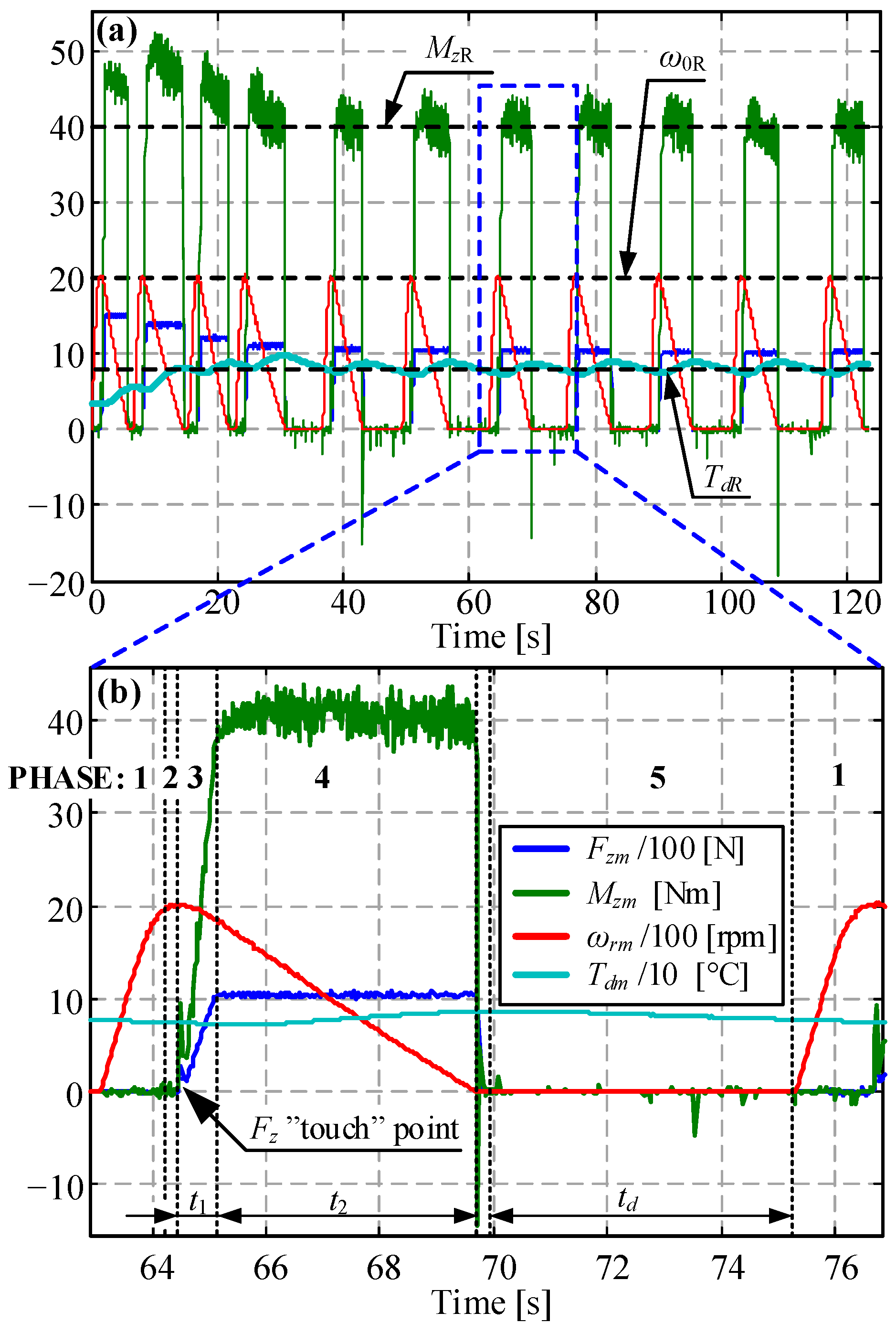
The wear tests are organized as a series of clutch closing cycles to mimic the operation of real manual transmission clutch. Each closing cycle consists of five phases (see Figure 2, [25]): (1) ramping up the slip speed to the target initial value ω0R under idling conditions, (2) lowering the vertical axis through closed-loop position control until the friction contact is established, (3) ramping up the normal force through closed-loop force control (interval t1), (4) maintaining the normal force at the target level FzR until the clutch stops (interval t2), and (5) lifting up the vertical axis followed by a cooling delay (interval td).
The torque, slip speed, temperature, and closing time are accurately controlled via feedback controllers acting through rotational- and vertical-axis servo drives and the water-cooling system (see time responses in Figure 2 and [25] for more details). The heat needed to increase the friction interface temperature is generated by friction itself and, thus, a certain number of closing cycles are needed to reach the target temperature TdR. The temperature is controlled by means of time delay td imposed between two consecutive clutch closing cycles, as well as by varying the cooling pump speed and manipulating an on/off valve that bypasses the coolant flow around the pressure plate. The torque is controlled at the target level MzR by using an integral (I) controller that commands the normal force reference (FzR) to a cascade closed-loop force controller. So-called electric inertia is added through the rotational axis motor to control the clutch closing time. For this purpose, an I-type closing time controller is employed to command an electric inertia ratio, which is used to calculate the rotational axis servomotor torque reference from the measured friction interface torque. Several closing cycles are generally needed to settle the torque and closing time at their target values (Figure 2).

3. Design of Wear Characterization Experiments

3.1. Static Experiments

Wear characterization experiments are conducted as a series of clutch closing cycles characterized by the target values of the following four closed-loop controlled operating parameters (see Section 2): clutch temperature ( T d R ), initial slip speed ( ω 0 R ), closing time ( t 2 R ) and clutch torque ( M z R ). The wear rate w is defined as the ratio of clutch worn volume V w (expressed in mm3) and corresponding cumulative dissipated energy (expressed in MJ):
w = V w / i = 1 n E d i s , i   [ mm 3 / M J ] ,
where n represents the number of considered closing cycles with the same operating parameters, and E d i s , i is the dissipated energy during the ith cycle.
Three distinctive levels of each operating parameter are considered: T d R 120 ,   170 ,   240   ° C , ω 0 R 1200 ,   1700 ,   2800   r p m , t 2 R 0.9 ,   2.15 ,   3.4   s , M z R 25 ,   50 ,   75   N m . The basic/initial design of experiments (DOE) is derived from all combinations of individual parameters’ levels (i.e., full factorial design), resulting in 34 = 81 experimental operating points in total (characterization points shown by blue circles in Figure 3). Operating parameters of several characterization points are adjusted (see, e.g., empty blue circles), since they could not be executed due to the test rig limitations. Additional 20 interpolation points are derived from the target operating space by maximizing their distance from the basic 81 points (green circles in Figure 3). Finally, 20 extrapolation points (red circles in Figure 3) are placed outside of the target operating space and close to the edge of individual parameters’ feasible operating region. The characterization and extrapolation points are used for wear rate model parameterization (modeling points), while the interpolation points serve as a basis for model validation.

3.2. Run-In Experiments

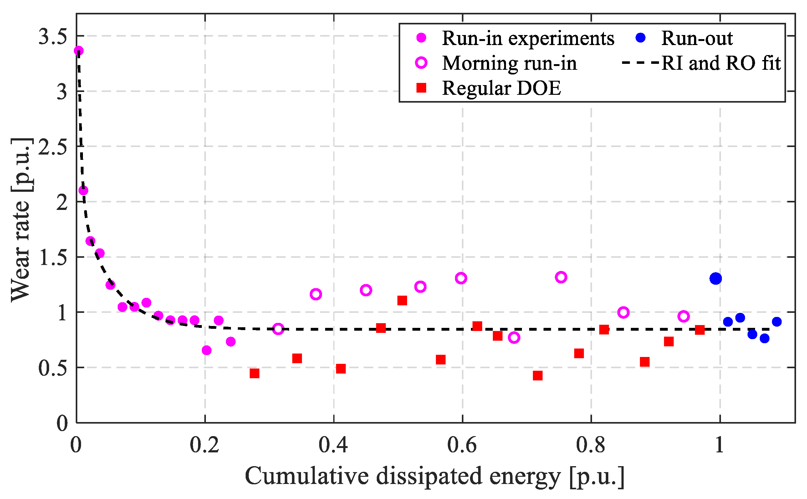
The wear rate is naturally increased in the initial, so-called run-in phase (see Figure 7 and Section 4). To characterize the run-in behavior, each tested friction plate was initially exposed to run-in experiments for the fixed (run-in) operating point: ω0R = 2800 rpm, MzR = 50 Nm, t2R = 3.4 s, TdR = 170 °C until a stabilized wear rate is reached (Figure 4 [25]). The same experiments were also conducted in the final phase, i.e., just before the friction lining was worn-out (so-called run-out (RO) phase; blue points in Figure 4), in order to serve as a basis for analysis and compensation of wear rate variability among different friction plates (so-called piece-to-piece variation) [26]. The interval between run-in and run-out phases was used for regular wear rate characterization experiments (filled red rectangles in Figure 4). Depending on a combination of operating parameters, between 3 and 14 operating points were recorded per one friction plate, and 13 friction plates were worn out in total to complete all 121 experiments from Figure 3 (see Figure 5). Note that the wear rate and the corresponding dissipated energy values are shown in Figure 4 and throughout the paper in a normalized (per unit; p.u.) form.
Each wear rate point in Figure 4 was recorded after a certain, relatively large number of closing cycles was executed on the tribometer test rig. Plate mass measurements were conducted before and after each wear rate point tests to derive the corresponding worn mass m , which yielded worn volume as V w = m / ρ , with ρ denoting the measured friction material density. The cumulative energy dissipated during the same interval, E d i s , i , was calculated from the slip speed and torque responses, and it was finally used to calculate the wear rate as: w = m / ρ i = 1 n E d i s , i [25] (see Equation (1)). The number of closing cycles n was determined based on the requirement that the worn mass would be at least 0.3 g to minimize the scale measurement imprecision influence. To suppress the wear rate variance (see Appendix A), the number of closing cycles was additionally limited to the minimum value set to a relatively high value of nmin = 750 cycles.
Since the friction material was hydroscopic, several measures were taken to minimize the moisture influence on the mass and, thus, wear rate measurement [27]: (i) the operating parameters imposed on a single friction plate had all the same temperature target level, (ii) each friction plate was stored overnight in a sealed container with a silica gel and dried in an electric oven for one hour at 100 °C at the start of each workday, (iii) prior to recording the first characterization experiment (i.e., after the oven drying), a one-hour preparatory experiment was carried out at the target temperature level (other inputs are set to their run-in values) to heat up the machine and thermally precondition the friction plate (see non-standard run-in empty magenta circle points in Figure 4), and (iv) the first regular characterization experiment weight difference in the workday was determined from the weight measurements recorded after the preparatory experiment and the subsequent wear characterization experiment (the first red square after the empty magenta circles in 4).

3.3. Cycle-Wise Validation Experiments

To mimic real-world driving operation, an additional set of more dynamic validation experiments has been carried out. An example of cycle-wise time traces of the input parameters during the overall validation experiment is shown in Figure 6. Each trace point corresponds to a single clutch closing cycle and represent the actual cycle value in the case of ω0 and t2 and the mean value in the case of Td and Mz (averaged over the closing time t2). Again, standard run-in experiments were first recorded for a new friction plate to stabilize the wear rate, and the standard run-in point was recorded at the start of each day. Then, instead of the static wear rate characterization experiments, where a single combination of operating parameters had been used, operating points were selected randomly from the full set of 121 operating points from Figure 3. Only the mechanical parameters were imposed (initial slip speed, torque, and closing time), while the temperature was left to float as in real clutch. Exceptionally, to suppress the clutch temperature excursions into low and high temperature regions over longer periods of time, the bypass valve was manipulated when the temperature exceeded the limits set to [100, 170] °C and [150, 240] °C for low-mid and high temperature conditions, respectively. Finally, the run-out experiments were recorded at the end of clutch life to characterize the piece-to-piece wear rate variability level.
Each randomly selected operating point was kept over 10 closing cycles, prior to switching to another operating point. There were 1500 closing cycles recorded in each day during the regular cycle-wise validation phase. They were executed in six blocks of 250 cycles (see Figure 6), where 1/3 of them corresponded to the high-temperature region and the rest to the low-mid temperature region. Finally, three blocks of 250 run-out cycles were performed (under run-in operating conditions), in order to stabilize the moisture content prior to wear-related mass measurement. In total, seven series of validation traces were recorded for a single friction plate (seven-day test, Figure 6). Every series had different sequences of low-mid temperature and high temperature limit blocks, but they were always in the ratio 2/3:1/3 of total closing cycles. Finally, to provide an ultimate mass measurements reliability over the full course of wear test, another friction plate was exposed to cycle-wise validation but at the constant (run-in) temperature conditions.

4. Wear Rate Characterization

4.1. Inherent Wear Rate Variability

As demonstrated by the response shown in Figure 7a, the clutch wear is characterized by a certain, inherent variability, i.e., the post-run-in wear rate varies under fixed operating conditions (blue points). The corresponding normal probability plot of wear rate residuals (Figure 7b) calculated with respect to wear rate response fitting curve (by using Matlab function normplot(.)) and the corresponding normality Lilliefors test (p value larger than a threshold 0.05; obtained by Matlab function lillietest(.)) indicate that the residuals are distributed according to normal distribution. This may be taken as a confirmation that there are no systematic test errors, i.e., the remaining sources of wear rate variability are of random nature, e.g., due to heterogeneity of friction plate composite material through the wear depth [27].

4.2. Wear Rate Variability Among Different Friction Plates

The run-in effect is reflected in the wear rate being several times higher at the beginning of clutch life than at the end of life (Figure 4 and Figure 7a). There are several physical mechanisms behind this effect. At the beginning of the clutch plate service life, the friction surfaces are not fully conformed, leading to localized areas of increased temperature and, consequently, elevated wear [28]. The rise in temperature accelerates the degradation of the resin matrix in the composite material, contributing to wear. Additionally, the organic material is prone to oxidation, which increases wear in surface layers that remain exposed to air for prolonged periods before first clutch/vehicle use.
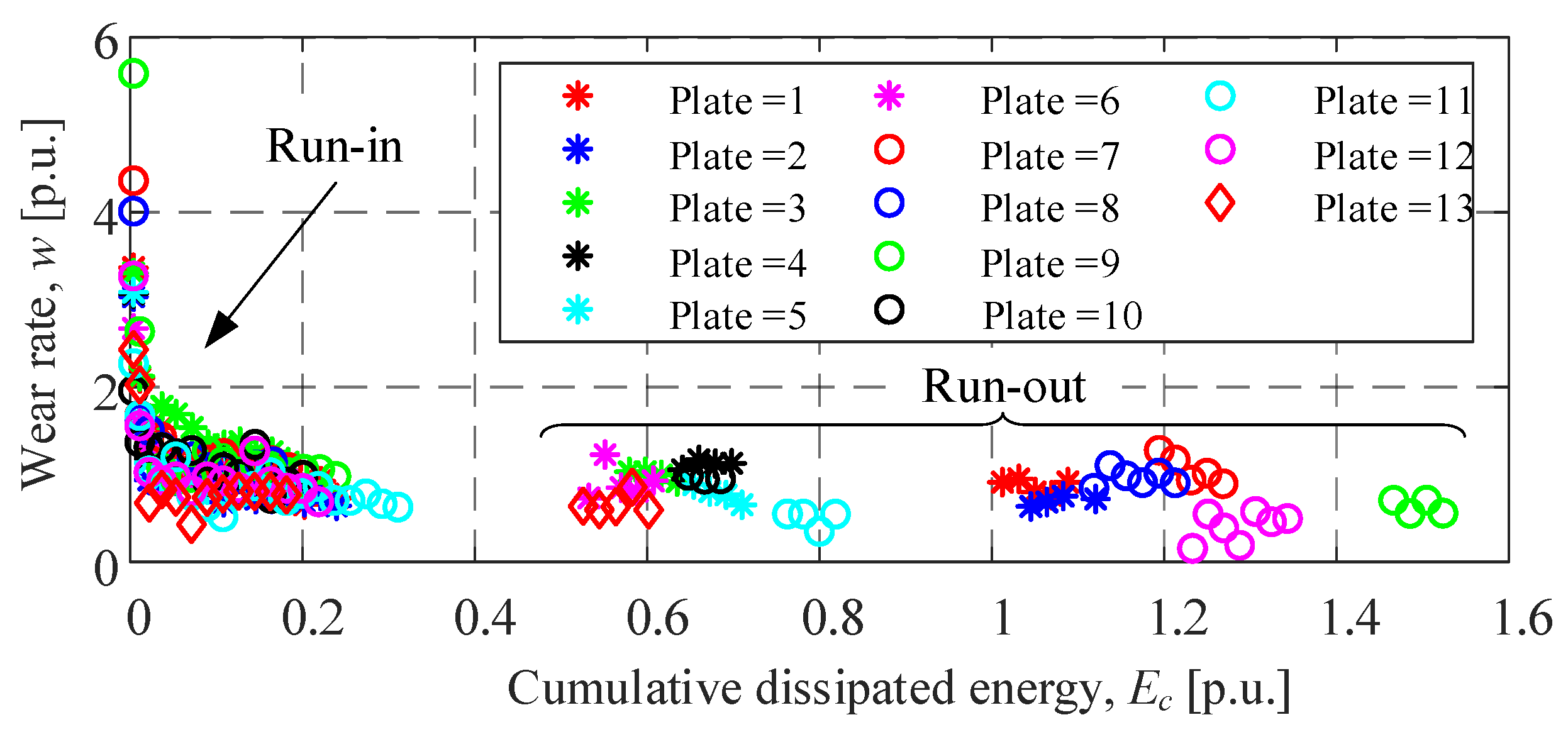
To investigate and model the run-in effect, the run-in and run-out recordings obtained for 13 tested friction plates have been considered. The results shown in Figure 8 indicate rather significant variability among the friction plates (piece-piece variability), which is caused by the heterogeneity and production variations in the friction plates.

4.3. Wear Rate Dependences on Individual Operating Parameters

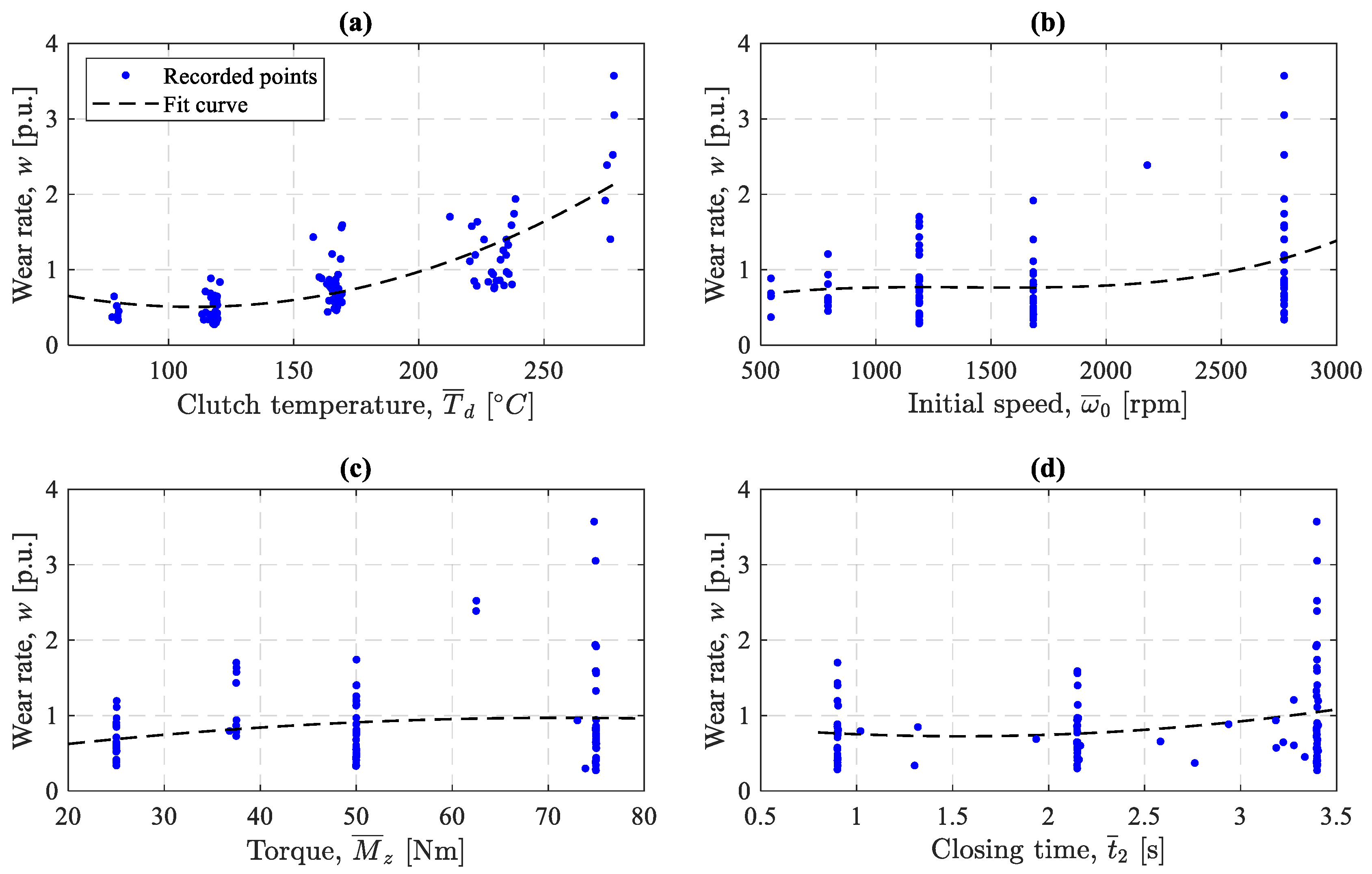
Visual inspection of the recorded wear rate characterization data related to all the operating points from Figure 3 has been performed to gain preliminary insights into the wear rate dependence on individual operating parameters. The parameter inputs T ¯ d ,   ω ¯ 0 ,   M ¯ z ,   a n d   t ¯ 2   are calculated as average values of the cycle-wise parameters over the full set of n cycles recorded for a specific operating point. The operating point dependence plots of wear rate are shown in Figure 9, along with corresponding low-order polynomial fit lines (dashed black lines). The related correlation indices (obtained by Matlab function corr(.)) are given in Table 1. Evidently, the temperature has the most dominant, progressive influence on the wear rate (Figure 9a) with the correlation coefficient of 0.744. The slip speed is somewhat less influential with the correlation index of 0.295 (Figure 9b), while the two remaining inputs, the clutch torque and the closing time, appear not to have significant influence (Figure 9c,d), with the correlation indices of 0.21 and 0.173, respectively. However, although having marginal influence when analyzed individually, the last two parameters may influence wear rate in combination with other parameters (i.e., in a nonlinear interactive manner; see Section 6 for more details).

5. Clutch Wear Model and Its Run-In Submodel

5.1. Model Structure

Since in real vehicles, particularly those equipped with manual transmission, the clutch operates in closing cycles, the wear model is designed to be executed in a cycle-wise manner. As the current clutch wear state estimate is of central interest, the cumulative worn volume ( V w ) is set to be the model output. To capture inherent wear rate variability, it is assumed that the wear rate for kth closing cycle is a random variable following a normal distribution (see the experimental evidence in Figure 7b) and having the expectation w μ , k and the standard deviation w σ , k dependent on the operating parameters. The related worn volume increment V w , k then follows a normal distribution, as well, with the expectation and variance parameters V w , μ k and V w , σ k 2 obtained by multiplying the related wear rate parameters with the dissipated energy E d i s , k :
V w , k ~ N w μ , k E d i s , k V w , μ k , w σ , k E d i s , k 2 V w , σ k 2 .
The total worn volume after a certain number of cycles can be obtained by summing up the corresponding worn volume increments:
V w k = V w , 1 + V w , 2 + + V w , k ~ N l = 1 k V w , μ l V w , μ k , l = 1 k V w , σ l 2 V w , σ 2 k .
where the worn volumes of individual cycles are assumed to be statistically independent (see the mathematical background in Appendix A). Taking the square root of variance yields the total worn volume standard deviation V w , σ , which can be used for calculating related worn volume 95% confidence interval (CI) as V w , μ ± 2 V w , σ .
To execute the wear model in a cycle-wise manner, the four operating parameters (initial slip speed ω0, clutch torque Mz, clutch temperature Td, and closing time t2, updated in each closing cycle; see Section 3 and Figure 6) would represent the model inputs that should be measured or estimated. To reduce the input space dimensionality and, thus, simplify the modeling process, the initial slip speed ω 0 and closing time t 2 are merged into a so-called surrogate distance input d s = ω 0 r t 2 q , with the exponents r and q being optimized for a favorable modeling accuracy (see Appendix B). The dissipated energy is calculated from the measured slip speeds and torques in each (ith) sampling step of the (kth) closing cycle and summed up over the total number of sampling steps (M):
E d i s k = i = 1 M M z i ω i t i t i 1 .
The cumulative dissipated energy Ec can then be calculated as:
E c k = l = 1 k E d i s l .
The wear model derived from Equations (2), (3) and (5) is shown in the form of block diagram in Figure 10. It consists of three main submodels: (i) run-in model providing a wear rate weighting function g (Ec) > 1 to account for the increased wear rate during the run-in period, (ii) wear rate expectation model with the output w μ , 0 , and (iii) wear rate variability model providing the wear rate standard deviation w σ . The expected wear rate w μ , 0 is multiplied by the run-in weighting function g (Ec) to obtain the actual/corrected wear rate w μ . The expectation of total cumulative worn volume V w , μ k after kth cycle is then updated through integration process (see the discrete-time integrator element 1/(z − 1)) as:
V w , μ k = V w , μ k 1 + w μ k E d i s k ,
where the worn volume is initialized to zero, i.e., V w , μ 0 = 0 . It should be noted that Equation (6) represents a recursive variant of Equation (3). Similarly, the total cumulative worn volume variance V w , σ 2 is updated based on the wear rate standard deviation prediction w σ (see Appendix A):
V w , σ 2 k = V w , σ 2 k 1 + w σ k E d i s k 2 .
The total worn volume standard deviation is then simply calculated as: V w , σ k = V w , σ 2 k .

5.2. Run-In Model

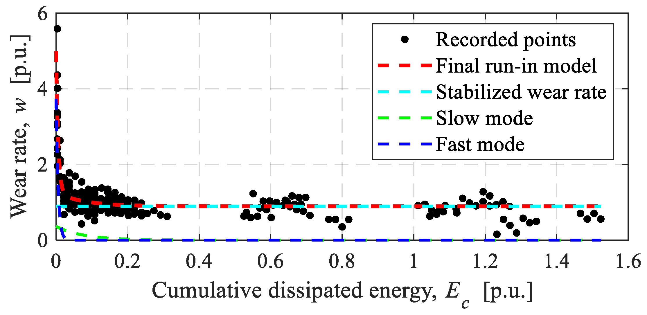
The run-in response from Figure 8 is modeled by a two-mode exponential function:
w E c = w 0 S t a b i l i z e d   v a l u e + w 1 e E c ε 1 S l o w   m o d e + w 2 e E c ε 2 F a s t   m o d e ,
where E c is the cumulative dissipated energy given by Equation (5), ε 1 and ε 2 are the energy constants representing the transient dynamics (the lth transient mode, l = 1, 2, is considered to diminish when the cumulative energy exceeds the value 3 ε l ), w 0 is the stabilized (steady-state) wear rate value, and w 1 and w 2 are the factors determining relative importance of individual modes. These parameters are obtained through optimization using Matlab function lsqcurvefit(.), applied to all run-in and run-out points of the tested friction plates (see Figure 11). The energy constant of the dominant, slower mode ε 1 was found to be around 13 times larger than the one of the faster mode ε 2 . On the other hand, the faster mode gain w 2 is about 10 times larger than the slower mode gain w 1 . Thus, the faster mode is characterized by a high-amplitude and low duration peak (Figure 11). It diminishes after the dissipated energy exceeds 0.03 p.u., while the less-dominant slow mode lasts up to the dissipated energy of around 0.35 p.u. (Figure 11).
The run-in weighting function g (Ec) appearing in the model in Figure 10 is determined by normalizing the run-in model (8) with respect to stabilized value w 0 :
g E c = w E c / w 0 .

6. Wear Rate Expectation Model

6.1. Model Structure

It is hypothesized that the wear rate expectation can be modeled with low-order polynomial functions. The hypothesis is supported by the initial insights into experimental data given in Figure 9 and the preliminary modeling results published in [26]. More general models, e.g., those based on advanced machine learning techniques, are less appealing in this application due to the low amount of recorded data available for model training (only 121 points, Section 3). The following general three-input full cubic model structure is selected:
y ^ = β 0 + β 1 x 1 + β 2 x 2 + β 3 x 3 + β 12 x 1 x 2 + β 13 x 1 x 3 + β 23 x 2 x 3 + β 11 x 1 2 + β 22 x 2 2 + β 33 x 3 2 + β 123 x 1 x 2 x 3 + β 112 x 1 2 x 2 + β 113 x 1 2 x 3 + β 122 x 1 x 2 2 + β 133 x 1 x 3 2 + β 223 x 2 2 x 3 + β 233 x 2 x 3 2 + β 111 x 1 3 + β 222 x 2 3 + β 333 x 3 3 ,
where there are 20 free ( β ) parameters and the total number of 220 − 1 = 1,048,575 submodels contained (each with unique combination of included terms). The general model inputs x 1 , x 2 , and x 3 (i.e., independent predictor variables) are used to form the input features z i ,   i 1 ,   2 , ,   20 , which are multiplied by the model parameters β i . The general model output, i.e., the dependent response variable is denoted as y ^ . In the context of the wear rate model, the three inputs correspond to operating parameters averaged over the n cycles of each operating point (see Section 4 and Figure 9) the surrogate distance x 1 = d ¯ s = ω ¯ 0 r t ¯ 2 q the clutch temperature x 2 = T ¯ d , and the clutch torque x 3 = M ¯ z , while the output is the wear rate expectation y ^ = w μ . The process of averaging the time-varying parameter inputs introduces a modeling error, because the wear dependencies on parameter inputs are not linear. However, as demonstrated in Appendix D, the error is very small, and thus negligible, because of relatively small parameter inputs variations.
The optimal wear rate expectation model is found by the best subset selection method [29], i.e., by iterating over all 1,048,575 submodels of the full cubic model (10) and assessing them according to a predefined criterion. It should be noted that if four inputs were considered, i.e., the initial slip speed ω 0 and the closing time t 2 instead of the surrogate distance ds, the full cubic model would have 35 free parameters and the total number of 235 − 1 = 34,359,738,367 submodels, and the best subset selection approach would not be feasible. In that case, another model structure optimization method should be used [30].

6.2. Model Parametrization

The model (10) is linear in parameters, and it can effectively be identified by using the least square method [29]. The parameters of each submodel contained within a vector β are obtained by minimizing the following mean squared error (MSE) cost function:
β = argmin β 1 N j = 1 N w μ j β w j 2 ,
where N is the number of recorded points used for modeling (characterization and extrapolation points from Figure 3; N = 101), w μ j is the model-predicted wear rate expectation, and w j is the recorded wear rate for jth point of the modeling dataset. The parameters which minimize (11) are calculated as:
β = X T X 1 X T w ,
where w is the column vector containing recorded wear rate points, and X is the design matrix containing normalized features zj,i for the related submodel. The matrix row and column indices j and i, respectively, correspond to jth recorded point within the modeling dataset, j 1,2 , , N , and ith feature, i 1,2 , , 20 . The model features z j , i are normalized to the interval [0, 1] as:
z j , i , n o r m = z j , i z i , m i n z i , m a x z i , m i n ,
to obtain a well-conditioned design matrix X, where z i , m i n and z i , m a x correspond to minimum and maximum values of ith feature.
Assessment of different submodels and selection of the optimal one are based on the coefficient of determination R2 [31]:
R 2 = 1 j = 1 N w μ j w j 2 j = 1 N w j w ¯ 2 ,
where w ¯ is the mean wear rate among N recorded modeling points. The index R2 takes values in the range [0, 1]. It is often interpreted as a proportion of variation in the dependent response variable (here the wear rate) that is predictable from independent predictor variables. The maximum value R 2 = 1 corresponds to the idealized, zero-error model case.
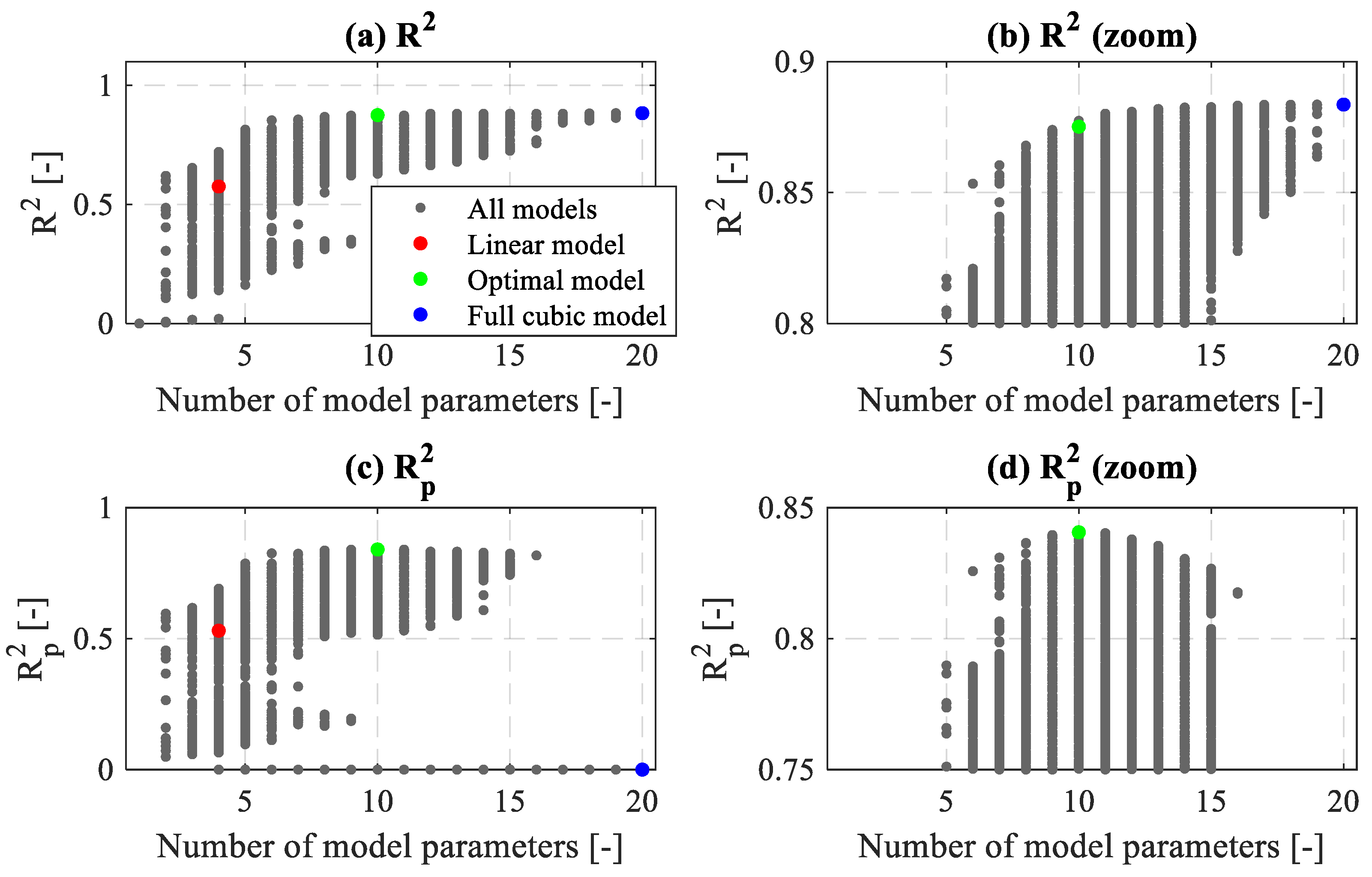
By successively adding model terms to the model, i.e., by enriching it with additional degrees of freedom, the R2 index typically improves (increases) when calculated over modeling points, because of an increase in model fitting capacity (see Figure 12a,b). However, at some number of model parameters, the model starts to fit noise present in the data, while degrading target input–output dependencies, which is known as overfitting [29]. To avoid overfitting, a leave-one-out cross-validation is performed [29], providing a so-called predicted R2 value, denoted below as R p 2 . The cross-validation procedure is as follows: (i) leave jth point from the modeling dataset and fit the model to remaining N − 1 points by using Equation (12), (ii) predict the wear rate by the model obtained in Point (i) for the removed jth point, w μ j , and calculate the related model error/residual ε j = w μ j w j , (iii) repeat Steps (i)–(ii) until obtaining model residuals ε j for all N points from the modeling dataset, and feed them into Equation (14) to obtain R p 2 . The overfitting avoidance is demonstrated in Figure 12 through comparison of R2 and R p 2 indices. Figure 12 also indicates that the model accuracy strongly depends on combination of input features and not only on their number.

6.3. Model Validation

The finally selected model structure which maximizes R p 2 index (Figure 12d) has ten parameters (out of maximum 20 parameters) and it reads:
w ^ = β 0 + β 1 d s + β 2 T d + β 12 d s T d + β 23 T d M z + β 33 M z 2 + β 123 d s T d M z + β 112 d s 2 T d + β 113 d s 2 M z + β 223 T d 2 M z .
The parameters of selected model (15) are finally re-calculated with respect to all modeling points (i.e., not with one point omitted). The model (15) reveals that the surrogate distance input influences the wear rate in a rather complex way, i.e., in several combinations with other inputs, with the highest influence found to be in combination with temperature T d (the parameters β 12 , β 112 , and β 123 take on high values; around 10 times larger than β 0 ). The temperature exhibits the highest individual influence and appears in several influential combinations with surrogate distance and clutch torque (the parameters β 2 and β 23 are also found to be about 10 times larger than β 0 ).
The optimal model (15) is validated against the following two distinct models based on R2, R p 2 , and root mean square error metrics RMSE and RMSEp: (i) a simple linear model: w ^ = β 0 + β 1 t 2 + β 2 T d + β 3 M z (four parameters), and (ii) a full cubic model involving all features (20 parameters). The comparative performance indices are given in Table 2 (see also Figure 12 for a wider response of indices R2 and R p 2 ). The selected, 10th-order model has a favorable accuracy characterized by rather high R2 and R p 2 values (not far from the ideal value of 1). A small gap between R2 and R p 2 indicates low level of overfitting of the modeling data. The low-order linear model has significantly lower R2 and Rp2 values, being around 0.55, and significantly larger residuals with RMSE being 1.85 times higher than that of the selected model. The full cubic is only slightly better in terms of R2 index (0.884 vs. 0.875), regardless of its significantly higher flexibility to fit the modeling data (20 vs. 10 parameters). On the other hand, the higher flexibility of the full cubic model leads to overfitting, as indicated by lower Rp2 value compared to the selected (optimal) model.
Table 3 includes the performance metrics of wear rate expectation model (15) with respect to validation points from Figure 3 (20 points not used in model parameterization). The R2 value of 0.411 is significantly lower than the corresponding value 0.875 obtained for modeling points. When omitting one of the validation points that appears to be an outlier (Point 13 in Figure 16b), R2 increases to 0.721, which is significantly closer to the value 0.875 obtained for modeling points. Also, the mean and standard deviation values of validation points’ residuals are rather comparable to those of modeling points (Table 3).

6.4. Model Analysis

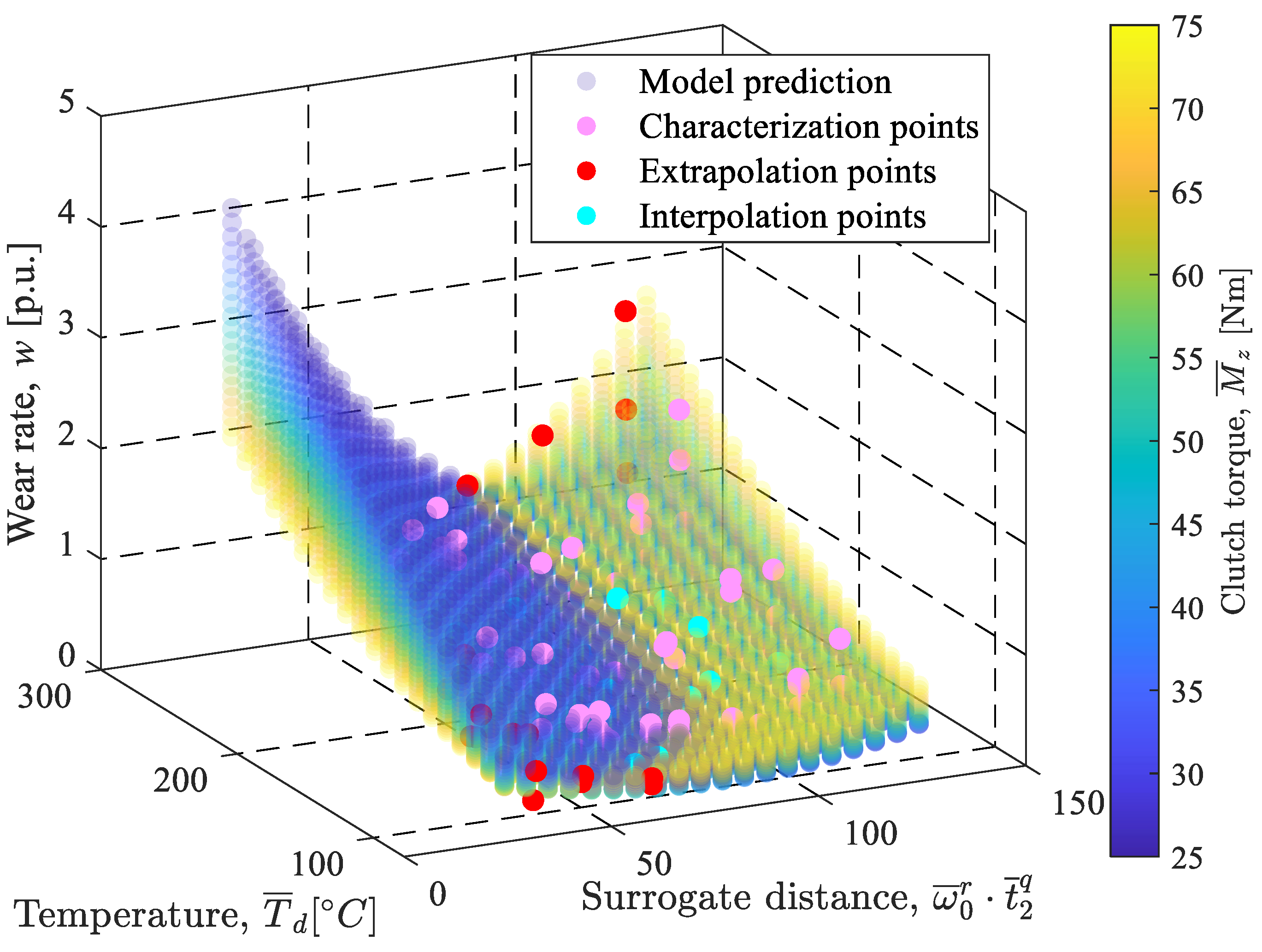
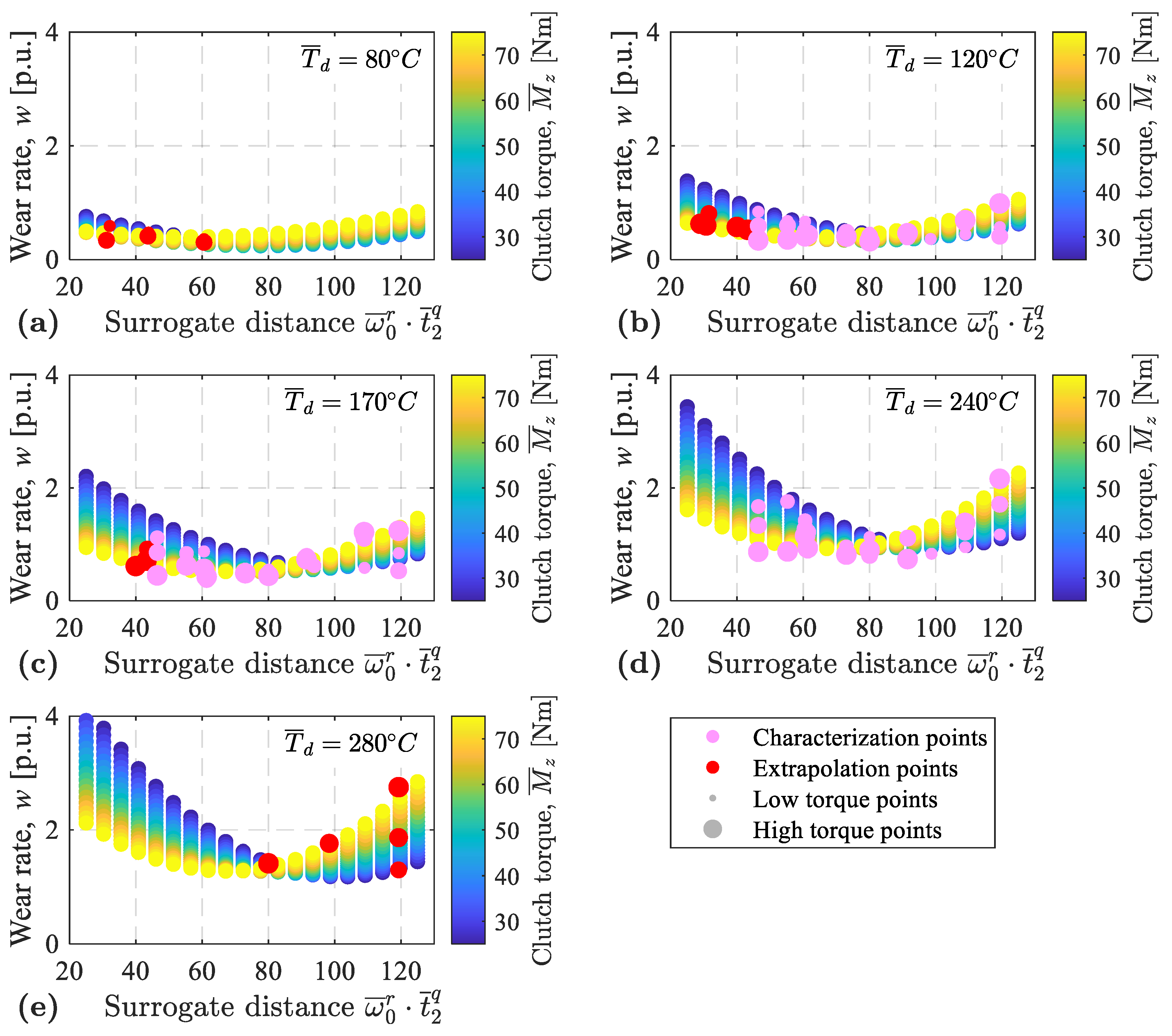
A 4D surface response of the selected 10-th order wear rate model is shown in Figure 13, along with the recorded points used for modeling. The corresponding 3D plots for different distinct temperatures are presented in Figure 14. The surface response in Figure 13 confirms progressive increase in the wear rate with clutch temperature (cf. Figure 9). The response with respect to surrogate distance shows a characteristic node point, at which the torque dependence of wear rate changes its trend from falling to rising one (see change in surface color in Figure 13 and Figure 14). The node point appears around the middle of surrogate distance range. The overall accuracy of matching the recorded data is very good. Note that there are no recorded points for high surrogate distance and low temperature conditions (Figure 14a), which is due to a long cooling phase needed to keep the clutch temperature at high power dissipation conditions, thus making the related experiments to be infeasibly long. Also, there are missing recorded points in the high temperature/low surrogate distance range (Figure 14e), because it was unattainable to reach high target temperature under low power dissipation conditions.

6.5. Comparative Performance Analysis of Models for Three Friction Materials

The wear rate modeling method described above for one friction material (Material A) has been applied to two additional dry clutch friction materials from different manufacturers (Materials B and C). The same experimental procedure was followed, with 101 modeling points and 20 validation points recorded under identical operating conditions by using the same tribometer rig. The comparative model structure and performance data for both the modeling and validation datasets is presented in Table 4. All the friction materials’ models have similar number of model terms of the full cubic model. They are also characterized by comparative performance metrics, with the note that the performance of additional materials B and particularly C when evaluated on the validation dataset would not be better than that of basic material A if the outlier-like Point 13 is excluded from the basic material dataset (cf. Table 3). The solid and comparable modeling performance across all three materials demonstrates the generalizability of the modeling method.

6.6. Comparison with Baseline Model

To further illustrate the developed wear rate model accuracy and applicability, the model performance metrics are compared with the metrics of the common, baseline model having only temperature as the single, most influential input parameter. The results presented in Table 5 indicates that the standard deviation of residuals of proposed model is reduced by around 60% when compared to that of the baseline model for the modeling dataset, while the R2 index is increased from 0.583 to 0.875. The performance metrics are also considerably improved when considering the validation dataset if the outlier-like Point 13 is excluded from the dataset.

7. Wear Rate Variability Model

7.1. Modeling Approach

The wear rate variability submodel from Figure 10 has been developed by using the maximum likelihood method [32]. Based on the experimental evidence in Figure 7, the wear rate probability distribution for particular operating parameters is assumed to have normal distribution, where the mean is given by the wear rate expectation model and the standard deviation is to be provided by the wear rate variability model. The model parameters are determined by maximizing probability of capturing the recorded points used in the model parameterization dataset (characterization and extrapolation points from Figure 3). To this aim, a likelihood is used, which is defined as a value of probability density function (PDF) for a certain argument/input value (e.g., operating parameters used as inputs for the wear rate expectation model). Maximizing the following product of likelihood values of all (N) modeling points leads to maximization of probability of capturing the whole set of observed data points:
L Θ = f x 1 , y 1 , Θ · f x 2 , y 2 , Θ · · f x N , y N , Θ ,
where Θ is the vector of model parameters, y j is the observed, jth output value of a random variable accompanied with an input vector x j , f is a PDF providing the likelihood of occurrence of each x j , y j pair in dependence of parameters Θ . To avoid numerical issues, the multiplication of PDF values in (16) is typically transferred to a sum by taking its logarithm [32]. Furthermore, the minus sign is added to convert the problem from maximization to minimization. This finally results in the negative log likelihood (NLL) cost function to be minimized [29]:
L Θ = j = 1 N l o g f x j , y j , Θ .
The normal distribution PDF reads:
f x j ,   y j , θ =   1 σ x j , θ 2 π e 1 2 y j μ x j σ x j , θ 2 ,
where μ and σ are its expectation and standard deviation, respectively. In the context of wear rate modeling, y j represents the recorded wear rate w j , x j stands for the input operating parameters (e.g., T d , j , M z , j , ω 0 , j , t 2 , j ), μ j = μ x j is the wear rate expectation w μ j (see Section 4), and σ j = σ x j , θ is the wear rate standard deviation w σ , j to be modeled.
In the cost function (17), the residuals are calculated as the difference between recorded and model-predicted wear rate, w j w μ j . A certain downside of this approach is that the wear rate expectation modeling errors are added to the inherent wear variability meant to be captured by the variability model. The alternative could be to record multiple data points per a single set of operating parameters to directly characterize the wear rate variability (see example in Figure 7), but this would require an extensive number of friction plates to be worn out and infeasibly long overall test time. Such an alternative approach has been carried out on a limited scale to additionally validate the modeling method presented in this section (see Appendix C).

7.2. Optimization Procedure and Model Candidates

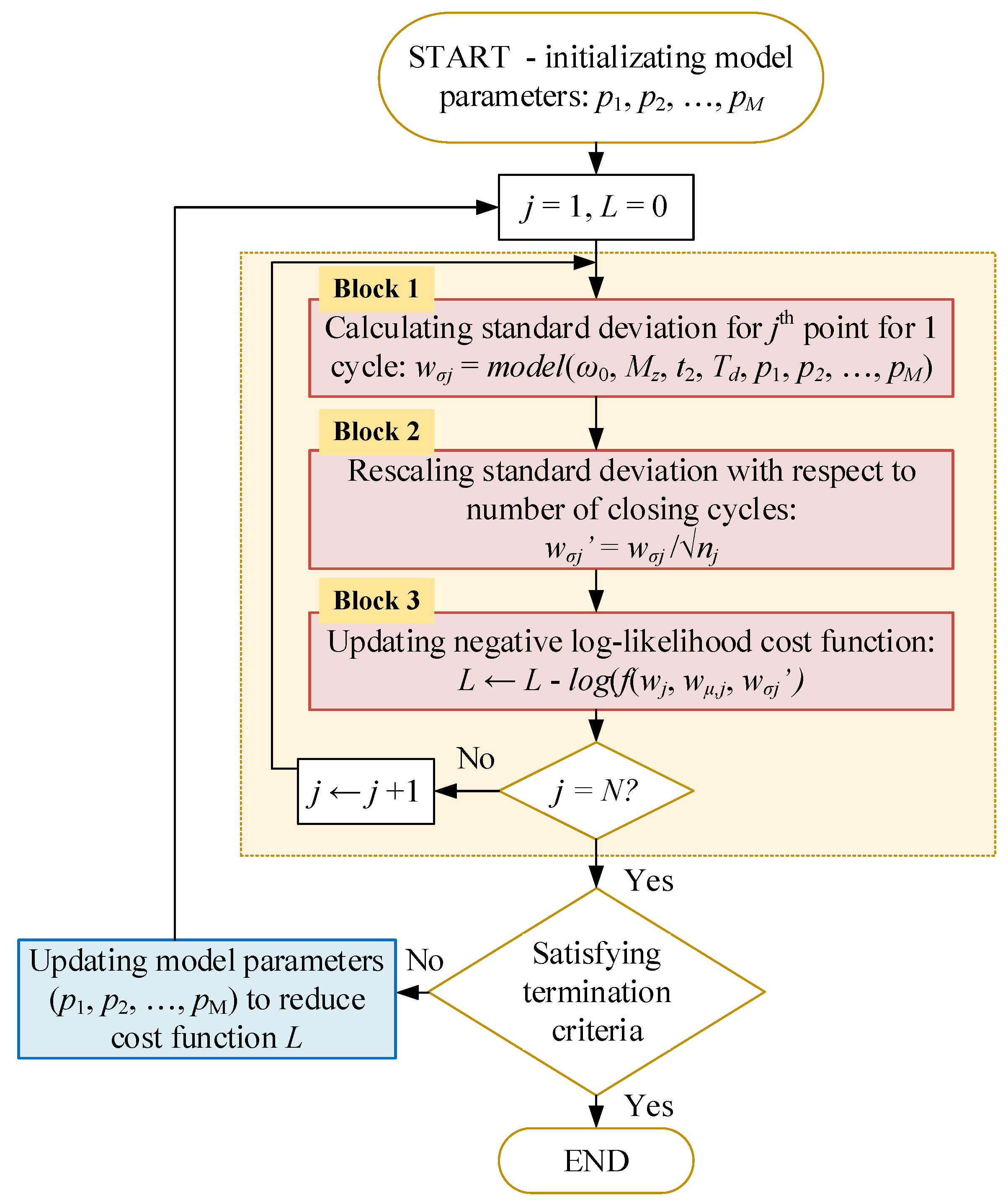
The procedure for optimizing the wear rate variability model parameters θ is described by the flowchart given in Figure 15. Firstly, the model parameters are initialized. The wear rate standard deviation w σ , j is then calculated for jth modeling point, by using a nominated variability model for the current operating parameters (Block 1 in Figure 15). To account for the influence of different number of repetitive closing cycles nj on wear rate variability for different operating points j = 1, …, N (see Appendix A, Figure 2 and Section 2), the modeled standard deviation is corrected as (Block 2)
w σ , j = w σ , j / n j ,
before inputting it to the NLL cost function (17) (Block 3). After iterating over all modeling points to obtain the NLL cost (17) for the current set of wear rate variability model parameters (inner loop in Figure 15), the parameter optimization algorithm is executed to provide a new set of model parameters aiming to further reduce NLL (outer loop in Figure 15). Matlab function fminsearch(.) is used to perform the model parameters optimization, which terminates the search when the cost improvement ceases. The determined standard deviation w σ , j can readily be used to obtain 95% wear rate CI for jth operating point: w μ , j ± 2 w σ , j = w μ , j ± 2 w σ , j / n j .
Several wear rate variability model candidates are nominated: (i) exponential, (ii) linear, and (iii) quadratic models taking the expected wear rate w μ as the only input (see Figure 10), as well as (iv) linear model with all operating parameters as inputs (Td, ω0, Mz, t2):
w σ = p 1 e p 2 w μ ,
w σ = p 1 + p 2 w μ ,
w σ = p 1 + p 2 w μ + p 2 w μ 2 ,
w σ = p 1 + p 2 T d + p 3 ω 0 + p 4 M z + p 5 t 2 .

7.3. Model Validation

The obtained 95% CIs are shown in Figure 16 along with recorded and expectation model-predicted wear rate values. An initial visual inspection reveals that 95% CIs of all variability models are similar, both for modeling (Figure 16a) and validation points (Figure 16b). The tight alignment of 95% CIs is reflected in similar cost function values in Table 6. The richest, multi-input model (22) expectedly provides the lowest cost function. The 95% CIs in Figure 16 embrace almost all tested points, thus pointing to the variability model accuracy. A distinct exemption is validation point #13, which may be considered as an outlier, (as performed in Section 4). Figure 16 also provides an additional, visual confirmation of expectation model validity discussed in Section 4: recorded vs. expected wear rate points fall around the ideal identity curve.
A joint analysis of model residuals and related variability model performance is hindered by the wear rate variability dependence on the operating point. The joint analysis is possible if the residuals are normalized with respect to corrected wear rate standard deviation:
ε s c a l e d , j = w j w μ , j w σ , j ,   j 1 ,   2 ,   ,   N .
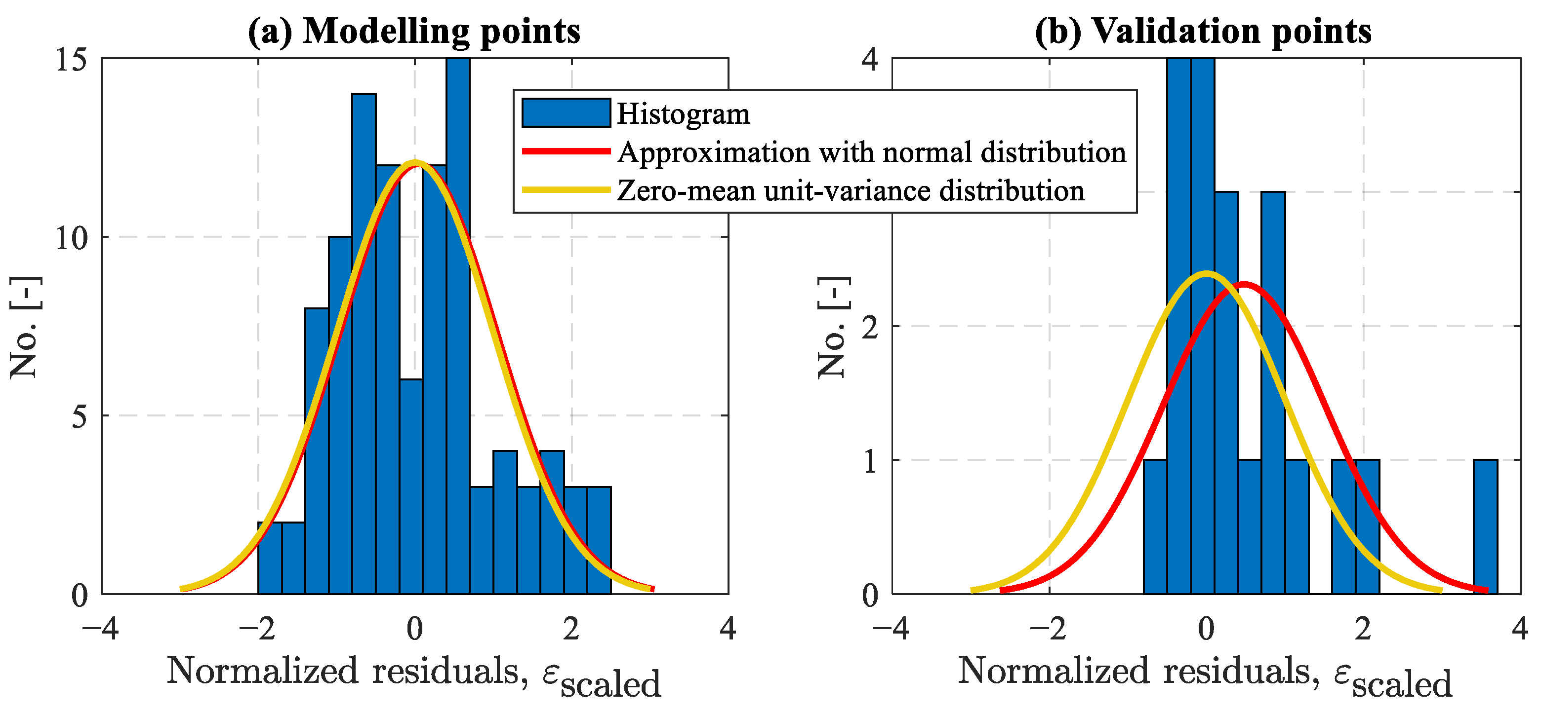
Mean and standard deviation of the residuals (23) are further denoted as ε s c a l e d , μ and ε s c a l e d , σ , respectively. If the model predictions w μ , j and w σ , j are accurate, the scaled residuals ε s c a l e d , j should distribute according to the standard normal distribution, with zero-mean ( ε s c a l e d , μ = 0 ) and unit standard deviation ( ε s c a l e d , σ = 1 ) [32]. Thus, the analysis of scaled residuals and related normality tests are used as a basis for additional variability models’ validation (note that the wear rate expectation model was already validated, see Table 3). For this purpose, Kolmogorov–Smirnov (KS) test is employed, which sets a null hypothesis that the collection of considered samples is drawn from the standard normal distribution to be true if related p value is larger than the threshold of 0.05. As shown in Table 6, all models satisfy the KS test, both for modeling and validation points, which is reflected in near-zero mean values ε s c a l e d , μ and near-unit standard deviations ε s c a l e d , σ . Also, the normal distribution fit curves corresponding to the normalized residual histogram data (obtained by Matlab function histfit(.)) align well with the standard zero-mean unit-variance distributions (rescaled to correspond to respective histograms, Figure 17). The normality of residuals may also be taken as an indicator that there are no considerable systematic errors of wear rate expectation modeling, i.e., that the related residuals captured by the variability model can be majorly attributed to inherent wear rate variability.

8. Validation and Analysis of Overall Wear Model

8.1. Model Validation

The proposed overall wear model from Figure 10 is validated in a cycle-wise manner, i.e., over consecutive closing cycles with time varying operating parameters illustrated in Figure 6, thus mimicking real-world clutch application. The quadratic wear rate variability model (21) is employed. The obtained experimental and model-based simulation responses of cumulative worn volume are shown in Figure 18 for two test plates, where Plate I experienced floating temperature and Plate II was for the constant temperature (see Section 3). They align very well with each other, with the simulation response falling within 95% CI over all closing cycles, except at the very beginning of the response characterized by uncertain run-in wear levels. The relative total worn volume modeling error amounts −3.76% and 5.95% for Plates I and II, respectively, which is well within the estimated 95% CIs at the end of responses being equal to ±11.1% and ±14.5%, respectively. The above results confirm the validity of the overall wear model under more realistic, dynamic conditions.

8.2. Model Analysis

For the sake of overall wear model response analysis, the response of absolute and relative width of 95% CI is calculated for the following predefined clutch plate wear levels: 10%, 20%, 50% and 100%. The friction plate is considered to be worn-out (the level of 100%) when the worn depth of friction material is equal to 1 mm. The run-in phase is omitted from the analysis and the modeling operating points are involved.
A preparatory procedure for calculating the worn volume 95% CI width is executed in two steps: (i) select the wear level x in percentage (e.g., 20%) and an operating point (among 101 modeling points from Figure 3), (ii) calculate the related wear rate expectation wμ and standard deviation wσ using the models (15) and (21), respectively, and determine the mean recorded dissipated energy per one cycle E1. The worn volume expectation and standard deviation per one cycle are then determined as: V w , μ , 1 = w μ E 1 and V w , σ , 1 = w σ E 1 , respectively, while after n x cycles they read: V w , μ = n x V w , μ , 1 and V w , σ = n x V w , σ , 1 (see Appendix A for mathematical background). Thus, the expected number of cycles needed to wear out the plate up to the selected level x [%] can be determined as:
n x = x 100 V w , t o t a l V w , μ , 1 ,
where V w , t o t a l is the fully worn plate volume.
The 95% CI of worn volume after n x cycles is defined as two standard deviations around the expected value V w , μ :
95 % C I V w n x = 2 V w , σ = 2 n x V w , σ , 1 .
The relative 95% CI width is calculated by dividing the above absolute width with the expected worn volume after n x repetitive cycles:
95 % C I r e l V w n x = 2 V w , σ V w , μ = 2 n x w σ E 1 n x w μ E 1 = 2 w σ w μ n x .
Hence, the absolute width of 95% CI is proportional to n x , while the relative width of 95% CI is inversely proportional to n x .
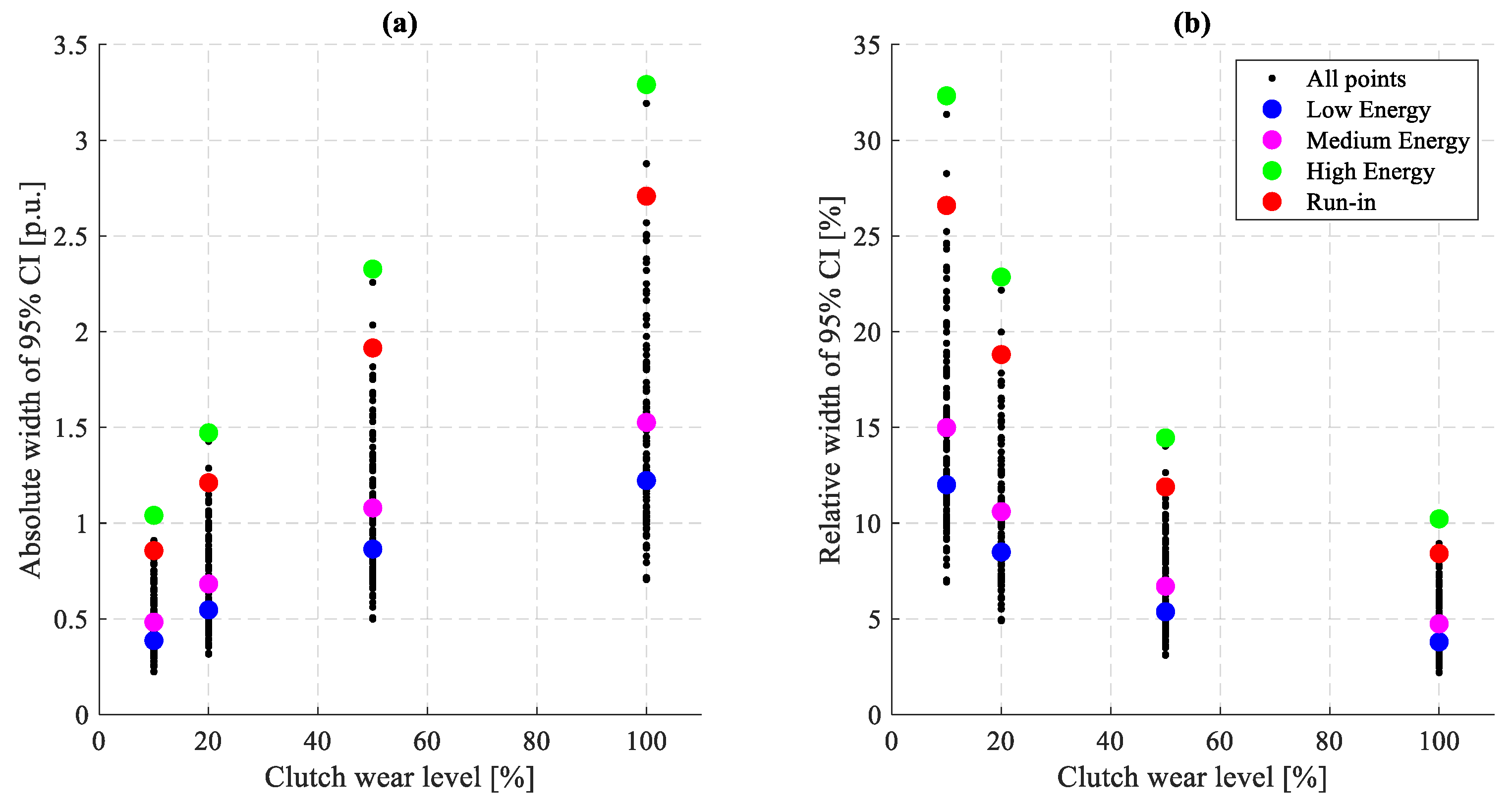
Figure 19 shows the absolute and relative widths of 95% CI for 101 modeling points from Figure 3 and the four wear levels. The same results are presented in Figure 20 in a different, wear response form. These results confirm that the absolute CI width grows with the wear level, while the relative CI reduces as the clutch is more worn. Hence, as the clutch wears out the confidence to the model prediction according to the expectation value reduces in the absolute sense, but it grows in the generally more relevant relative sense (see also validation results in Figure 18). The relative width ranges from around 7% to 33% for 10% wear level, but it falls down to low values in the range of around 3% to 10% for the fully worn-out plate. Figure 19 and Figure 20 also reveals that higher the expected wear rate, the larger is the wear rate (and worn volume) variability, both in absolute and relative 95% CI width sense (see monotonic rise in polynomial fit functions in Figure 19 and the CI trends in Figure 16a).

8.3. Implementation Aspects

The main application of the developed clutch wear model is for offline analysis and design purposes, e.g., predicting the wear depth across the vehicle fleet and clutch life for realistic (potentially customized) driving cycles for different statistical analyses to determine the friction lining depth, warranty terms, and similar. The cycle-wise wear model can also have direct online application targeted at monitoring the clutch wear depth through time and related reporting to driver, car service and/or vehicle manufacturer for driver style alert, maintenance warning, and real-time statistical analyses purposes.
To run the cycle-wise clutch wear model, all the four parameter inputs should be available online. The initial clutch slip speed information is readily available online from the available engine and driveline speed sensors. The actual slip speed information can further be used to determine the clutch closing time. The clutch torque can be reconstructed in prototype vehicles by using halfshaft torque telemetry systems. The acquired torque signal can be then used to tune and validate a clutch torque estimation algorithm to be used in production vehicles. To avoid the use of a complex multi-input clutch coefficient of friction submodel when calculating the torque [33], the clutch torque can be estimated through an engine load torque observer [34]. The engine torque input is typically estimated from available sensor information such as throttle position, engine speed, air mass flow, or fuel injection rate [35]. Similarly, the clutch friction interface temperature can be measured in prototype vehicles by using telemetry systems, and the acquired information can be used to parameterize multi-mass clutch thermal models to be employed online in production vehicles to estimate the temperature. The main temperature estimator inputs would be the clutch slip speed and clutch torque, whose product gives the clutch dissipated power, as well as clutch component and vehicle speed to determine the heat transfer coefficients, and similar [36,37].

9. Conclusions

Experimental characterization and data-driven modeling of dry clutch friction lining wear has been presented in the paper. The experiments were performed on a custom-made disk-on-disk tribometer mimicking real clutch operation with clutch temperature, initial slip speed, clutch torque, and closing time as closed-loop controllable operating parameters resulting in 121 static operating points. The clutch friction interface temperature was identified to be most influential parameter input, with correlation index of 0.744. The correlation indices with respect to initial slip speed, clutch torque and closing time were 0.295, 0.210 and 0.173, respectively. The developed data-driven model predicts the friction lining worn volume and is organized around three distinctive submodels, providing wear rate expectation, standard deviation and weighting function accounting for run-in effect.
The wear rate expectation is described by a cubic model with three inputs: temperature, torque, and a surrogate distance combining initial slip speed and closing time. The optimal model structure has been selected via best subset selection, leave-one-out cross-validation, and least squares parameterization. The final model, maximizing the cross-validation index R p 2 includes 10 out of 20 possible parameters. The R p 2 value of 0.841 demonstrates a significant improvement over the common, baseline model having the temperature as the only input which is characterized by the R2 value of 0.583. On a separate validation dataset, the R 2 index still has relatively high value of 0.721, compared to 0.462 for the baseline model, confirming the modeling consistency. The wear rate variability model was developed by the maximum likelihood approach and its validity was confirmed by the statistical Kolmogorov–Smirnov test, both for modeling and validation datasets.
The overall wear model has been experimentally validated throughout the wear depth under randomly varying operating parameters mimicking real driving conditions. Prediction error of worn volume at the end of friction lining life was 3.8% and 6% for plates experiencing floating and constant clutch temperature, respectively. The model-predicted 95% confidence interval (CI) embraces well the recorded worn volume samples throughout the wear depth, except at the very early stage of run-in phase. The 95% CI decreases in relative sense as the friction plate is wearing down. For the worn-out level of 10% the relative width of 95% CI ranges from 7 to 33% depending on the operating conditions, while it reduces to the range from 3 to 10% for the fully worn-out plate.

Author Contributions

Conceptualization, B.Š., M.H. and J.D.; methodology, B.Š., N.K. and A.T.; software, K.H. and B.Š.; validation, K.H.; formal analysis, K.H., M.H. and J.D.; investigation, K.H., B.Š., M.H., N.K. and J.D.; resources, A.T.; data curation, M.H.; writing—original draft preparation, K.H. and M.H.; writing—review and editing, B.Š. and J.D.; visualization, K.H.; supervision, B.Š., N.K., J.D. and A.T.; project administration, J.D.; funding acquisition, J.D. and A.T. All authors have read and agreed to the published version of the manuscript.

Funding

This research was funded by the Ford Motor Company under the internal funding program number DEPT2019-J075.6.

Institutional Review Board Statement

Not applicable.

Informed Consent Statement

Not applicable.

Data Availability Statement

The data presented in this study are available on request from the corresponding author. The data are not publicly available due to privacy issues.

Conflicts of Interest

Author Andreas Tissot was employed by the company Ford-Werke GmbH. The remaining authors declare that the research was conducted in the absence of any commercial or financial relationships that could be construed as a potential conflict of interest.

List of Mathematical Symbols and Abbreviations

d s Surrogate distance
E c Cumulative dissipated energy
E d i s Dissipated energy
F z Clutch normal force
g Run-in weighting function
L Negative log likelihood function
T d Friction interface temperature
T ¯ d Cycle-wise average pressure plate temperature
T d R Pressure plate temperature reference
m Mass of the friction plate
M z Clutch torque
M ¯ z Cycle-wise average clutch torque
M z R Clutch torque reference
n Number of clutch closing cycles
p i Wear rate variability model parameters
R 2 Coefficient of determination
R p 2 Leave-one-out cross-validation coefficient of determination
t 1 Time of ramping up the normal force phase
t 2 Clutch closing time
t ¯ 2 Cycle-wise average clutch closing time
t 2 R Clutch closing time reference
t d Cooling delay
V W Worn volume
V w , μ Worn volume expectation
V w , σ Worn volume standard deviation
V w , σ 2 Worn volume variance
w Wear rate
w μ Wear rate expectation
w σ Wear rate standard deviation
x i General model inputs
X Design matrix
y ^ Dependent response variable
z i Input features
β i Wear rate expectation model parameters
ε i Run-in model energy constants
ε s c a l e d Normalized model residuals
Θ Wear rate variability model parameter vector
ρ Friction material density
ω 0 Initial slip speed
ω ¯ 0 Cycle-wise average initial slip speed
ω 0 R Initial slip speed reference
AMTAutomated Manual Transmission
CIConfidence Interval
DCTDual Clutch Transmission
DOEDesign of Experiment
KSKolmogorov–Smirnov
MSEMean Square Error
NLLNegative Log Likelihood
PDFProbability Density Function
RIRun-in
RMSERoot Mean Square Error
RORun-out

Appendix A. Mathematical Background

A sum of n normally distributed independent random variables, X i ~ N μ i , σ i 2 ,   i 1 ,   2 , , n , is also a normal distribution given by X s u m = i = 1 n X i ~ N i = 1 n μ i , i = 1 n σ i 2 [32]. In the special case of all individual random variables having the identical distributions ( X i ~ N μ , σ 2 ,   i ), one obtains
X s u m = i = 1 n X i ~ N n μ , n σ 2 .
The average value of individual random variable realization is also a normally distributed random variable:
X a v g = 1 n i = 1 n X i ~ N μ , 1 n σ 2 .
Hence, the variance of X s u m increases proportionally with the number of individual random variables n, while the variance of X a v g diminishes proportionally with n. That is, the standard deviations of X s u m and X a v g are proportional to n and 1 n , respectively.
When referring to wear rate modeling, based on Equation (1) one obtains
w = 1 ρ i = 1 n m i i = 1 n E d i s , i ,
where m i and E d i s , i are the friction plate worn mass and the dissipated energy during ith closing cycle, respectively, and ρ is the friction plate density. The worn mass m i is assumed to be a random variable with normal distribution. By assuming that the corresponding dissipated energies are equal over a sequence of cycles for the same operating point/parameters: E d i s = E d i s , 1 = = E d i s , n , Equation (A3) can be rewritten as:
w = 1 ρ E d i s 1 n i = 1 n m i ,
where i = 1 n m i n can be related to the general random variable X a v g from Equation (A2). Thus, the accuracy of wear rate reconstruction is increased in terms of variance by increasing the number of closing cycles. This finding was used as a basis for setting the lower limit on the number of closing cycles in the design of experiments in Section 3.

Appendix B. Selection of Wear Rate Model Inputs

To reduce the number of wear rate model inputs for computationally simpler model structure optimization, merging of two (or even three) inputs into a single one has been considered, with the following candidates nominated: surrogate power ( M z p ω 0 r ), surrogate distance ( ω 0 r t 2 q ), and surrogate energy ( M z p ω 0 r t 2 q ). The clutch temperature Td remains to be an independent predictor variable, as it has the highest influence on wear rate (see Figure 9).
The optimization procedure of surrogate input exponents p, r, and q is executed in two levels. The high-level optimization is set to be responsible for nominating the exponent values and preparing related model inputs and features, while the low-level performs a feature selection [29] over the full cubic model to find the optimal model structure based on the criterion of maximizing the R p 2 value. In the high-level loop, all the perturbations of the values exponents p, r, q taken from the set 0.1 ,   0.2 ,   ,   3 were considered.
Firstly, to determine the optimal surrogate input set (including the exponent coefficients), modeling was performed for each temperature level separately. In this way, the number of model inputs is reduced to two or one (i.e., when excluding temperature), thus facilitating the best subset search. The results are given in Table A1, where the surrogate distance is shown to provide the best performance in terms of average R p 2 . To obtain a unique set of optimal surrogate distance model exponents r and q for all temperatures, the parameter optimization was repeated by using the sequential feature selection of three-input full cubic model (10) (Matlab function sequentailfs(.) is used with 5-fold cross-validation). Note that in this case the best subset feature selection is infeasible due to its multiple executions within the outer parameter search optimization loop.
Table A1. Values of R p 2 metrics for optimized models with different surrogate input sets and for different clutch temperatures.
R p 2 Surrogate Inputs
Temperature Level Power ,   M z p ω 0 r Distance ,   ω 0 r t 2 q Energy ,   M z p ω 0 r t 2 q
120 °C0.5650.6550.611
170 °C0.5490.5750.577
240 °C0.7530.6900.596
Average0.6220.6400.595

Appendix C. Direct Validation of Wear Rate Variability
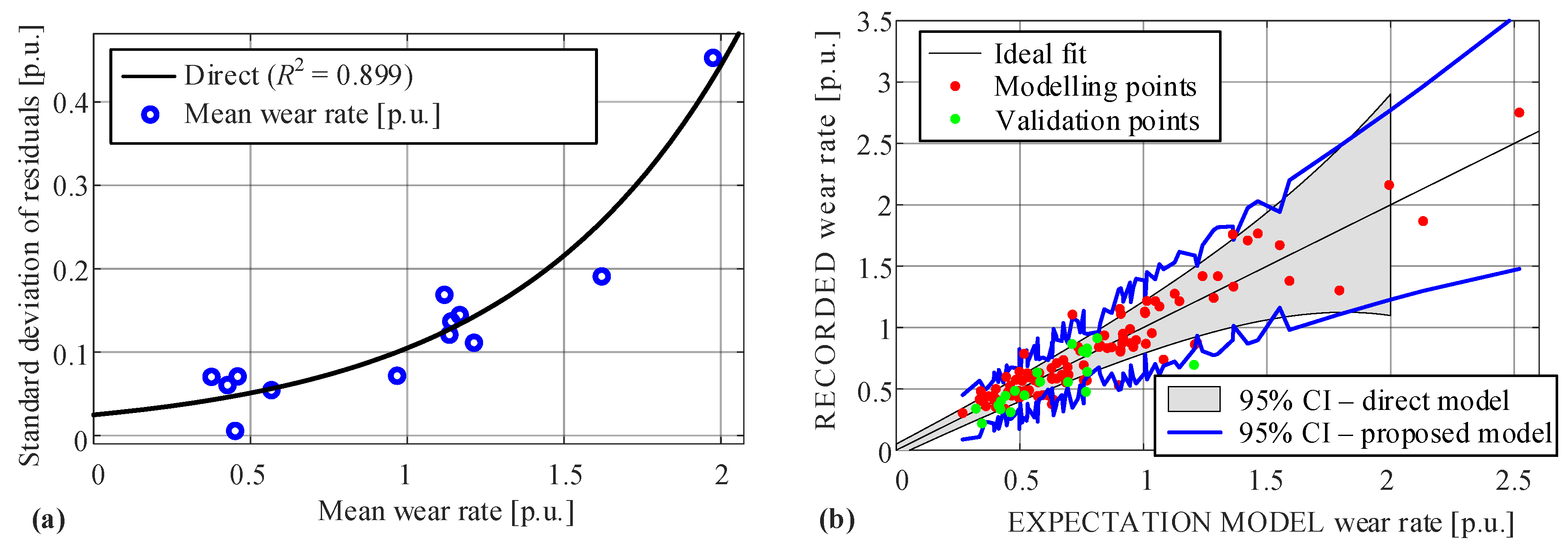
As noted in Section 7 and illustrated by Figure 7a, conducting long (e.g., full-depth) wear experiments for a fixed set of operating parameters can provide direct insight into inherent wear rate variability and a basis for direct validation of the variability model. Such experiments were conducted for a limited number of plates and operating parameter sets. The parameter sets had different initial slip speeds and temperatures (at the levels defined in Figure 3), while the torque and closing time were fixed to 50 Nm and 3.4 s, respectively.
Residuals with respect to mean wear rate value in the stabilized phase (see blue circles in Figure 7a) are used to calculate the respective standard deviation for each operating parameter set (blue circles in Figure A1a). As in the case of models given by Equations (19)–(21), only expected/mean wear rate is used as the model input, with an exponential function selected to fit the data (black line in Figure A1a). The related 95% CI, shown in Figure A1b (black lines), aligns rather well with the CI predicted in Figure 16 for the exponential model (19) (blue lines in Figure A1b), thus demonstrating validity of the proposed, more practical wear rate variability model from Section 7.
Certain differences between the two models in Figure A1b, i.e., somewhat narrower 95% CI of the direct model, may be explained by the following: (i) the experimental results in Figure A1a were obtained for different (earlier) batches of friction plates and an early, unrefined version of the tribometer rig than the ones used in the main body of this paper; (ii) the set of points in Figure A1a is rather limited in terms of number of points and their clustering in a couple of dominant regions (e.g., run-in operating conditions), (iii) the varying number of cycles in different tests (i.e., for different points in Figure A1a), which influences the wear rate variability (Appendix A), are not accounted for in the case of direct model, and (iv) the proposed model from Figure 16 can contain certain wear rate expectation modeling error that are reflected in the variability modeling inaccuracy (Section 7).
Figure A1. Wear rate variability model obtained from long, fixed operating parameter tests (a), and comparison of its 95% CI against that of exponential model from Figure 16, along with recorded modeling and validation points (b).
Applsci 15 08150 g0a1

Appendix D. Analysis of Wear Rate Modeling Error Due to Model Inputs Averaging

As described in Section 4 and Section 5, the model parameter inputs are averaged over n closing cycles when parameterizing and validating the wear rate model. Although the recorded parameter inputs are mostly close to their target levels throughout the wear rate characterization experiment, there are some deviations caused by slow temperature dynamics and corresponding changes in coefficient of friction (see, e.g., Figure 2). The highest deviation is for the first several closing cycles when the temperature has not stabilized yet.
Averaging parameter inputs allows for model parametrization using Equation (12) but introduces a wear rate modeling error as the wear dependence on parameter inputs is not linear. The modeling error can be quantified by using the developed cycle-wise wear prediction model (Figure 10). The model is firstly simulated with real parameter inputs recorded/averaged for every clutch closing cycle. This gives an accurate prediction of worn volume without averaging of input parameters. Secondly the cycle-wise model will be simulated for the same number of cycles, but the input parameters will be the same in every cycle and equal to average value of input parameters in the first simulation. The difference in worn volume between the two simulations corresponds to the modeling error due to inputs averaging.
The results of the analysis are shown in Table A3 for six operating points from Table A2 which covers a wide range of operating parameters. The average inputs-based model prediction error is very small, ranging from 0.1% to 0.65%. This error is at least by an order of magnitude smaller than the wear variability margins observed in Table 6 and Figure 16, Figure 17, Figure 18 and Figure 19.
Table A2. Definition of characteristic operating points used in analysis of wear rate modeling errors caused by model inputs averaging.
PointTemperature, TdR [°C]Initial Slip Speed, ω0R [rpm]Torque, MzR [Nm]Closing Time, t2R [s]
Low-energy, LE1701200253.4
Mid-energy, ME1701700502.15
Run-in, RI1702800503.4
High-energy, HE1702800753.4
Run-in @ 120 °C1202800503.4
Run-in @ 240 °C2402800503.4
Table A3. Results of analysis of wear rate modeling errors for operating points from Table A2.
PointWorn Volume for Recorded Inputs [p.u.]Worn Volume for Averaged Inputs [p.u.]Relative Worn Volume Difference
LE2.9032.901−0.080%
ME3.1003.092−0.240%
RI4.9394.930−0.175%
HE10.54410.511−0.317%
RI @ 120 °C3.3863.363−0.636%
RI @ 240 °C7.8747.861−0.160%

References

  1. Chen, Y.; Wang, X.; He, K.; Yang, C. Model reference self-learning fuzzy control method for automated mechanical clutch. Int. J. Adv. Manuf. Technol. 2018, 94, 3163–3172. [Google Scholar] [CrossRef]
  2. Shi, J.; Li, L.; Wang, X.; Liu, C. Robust output feedback controller with high-gain observer for automatic clutch. Mech. Syst. Signal Process. 2019, 132, 806–822. [Google Scholar] [CrossRef]
  3. Kob, M.; Supriyo, B.; Tawi, K.; Mazali, I. Engagement slip controller development based on actuator displacement for an electro-mechanical friction clutch system. Int. J. Automot. Mech. Eng. 2015, 11, 2664–2674. [Google Scholar] [CrossRef]
  4. Liauw, Y.; Roozegar, M.; Zou, T.; Morozov, A.; Angeles, J. A topology-change model of multi-speed transmissions in electric vehicles during gear-shifting. Mechatronics 2018, 55, 151–161. [Google Scholar] [CrossRef]
  5. Della Gatta, A.; Iannelli, L.; Pisaturo, M.; Senatore, A.; Vasca, F. A survey on modeling and engagement control for automotive dry clutch. Mechatronics 2018, 55, 63–75. [Google Scholar] [CrossRef]
  6. Pisaturo, M.; Senatore, A. Thermal Compensation Control Strategy in Automated Dry Clutch Engagement Dynamics and Launch Manoeuvre. Int. J. Automot. Technol. 2019, 20, 1089–1101. [Google Scholar] [CrossRef]
  7. Gong, T.; Yao, P.; Xiao, Y.; Fan, K.; Tan, H.; Zhang, Z.; Zhao, L.; Zhou, H.; Deng, M. Wear map for a copper-based friction clutch material under oil lubrication. Wear 2015, 328, 270–276. [Google Scholar] [CrossRef]
  8. Li, M.; Khonsari, M.M.; McCarthy, D.M.C.; Lundin, J. Parametric analysis of wear factors of a wet clutch friction material with different groove patterns. Proc. Inst. Mech. Eng. Part J J. Eng. Tribol. 2017, 231, 1056–1067. [Google Scholar] [CrossRef]
  9. Abdullah, O.I.; Schlattmann, J. Temperature analysis of a pin-on-disc tribology test using experimental and numerical approaches. Friction 2016, 4, 135–143. [Google Scholar] [CrossRef]
  10. Basavarajappa, S.; Ellangovan, S. Dry sliding wear characteristics of glass-epoxy composite filled with silicon carbide and graphite particles. Wear 2012, 296, 491–496. [Google Scholar] [CrossRef]
  11. Kim, S.; Jang, H. Friction and wear of friction materials containing two different phenolic resins reinforced with aramid pulp. Tribol. Int. 2000, 33, 477–484. [Google Scholar] [CrossRef]
  12. Ma, Y.; Wu, S.; Tong, J.; Zhao, X.; Zhuang, J.; Liu, Y.; Qi, H. Tribological and mechanical behaviours of rattan-fibre-reinforced friction materials under dry sliding conditions. Mater. Res. Express 2018, 5, 035101. [Google Scholar] [CrossRef]
  13. Fukuda, K.; Morita, T. Physical model of adhesive wear in early stage of sliding. Wear 2017, 376, 1528–1533. [Google Scholar] [CrossRef]
  14. Chi, H.T.; Jiang, L.T.; Chen, G.Q.; Kang, P.C.; Lin, X.; Wu, G.H. Dry sliding friction and wear behavior of (TiB2 + h-BN)/2024Al composites. Mater. Des. 2015, 87, 960–968. [Google Scholar] [CrossRef]
  15. Kumar, I.A.; Kumar, A.; Srinivasan, V.; Raffi, N.M. Wear Study on Basalt, Flax and Hybrid Fiber Reinforced Phenolic Composites. J. Adv. Microsc. Res. 2018, 13, 65–71. [Google Scholar] [CrossRef]
  16. Fernandez, G.; Zanotto, P.; Sinatora, A. Tribology Applied on Development of New Materials for Dry Clutch System. In Proceedings of the 8th Brazilian Congress of Manufacturing Engineering, Salvador, Bahia, Brazil, 18–22 May 2015. [Google Scholar]
  17. Biczo, R.; Kalacska, G.; Mankovits, T. Effects of Automotive Test Parameters on Dry Friction Fiber-Reinforced Clutch Facing Surface Microgeometry and Wear. Polymers 2021, 13, 3896. [Google Scholar] [CrossRef]
  18. Kulkarni, A.; Mahale, R.; Kannan, C. Wear Based Lifetime Estimation of a Clutch Facing using Coupled Field Analysis. Int. J. Automot. Mech. Eng. 2021, 18, 9292–9304. [Google Scholar] [CrossRef]
  19. Grzelczyk, D.; Awrejcewicz, J. Wear Processes in a Mechanical Friction Clutch: Theoretical, Numerical, and Experimental Studies. Math. Probl. Eng. 2015, 2015, 725685. [Google Scholar] [CrossRef]
  20. Li, M.; Khonsari, M.M.; Lingesten, N.; Marklund, P.; McCarthy, D.M.C.; Lundin, J. Model validation and uncertainty analysis in the wear prediction of a wet clutch. Wear 2016, 364, 112–121. [Google Scholar] [CrossRef]
  21. Tabbai, Y.; Alaoui-BeIghiti, A.; El Moznine, R.; Belhora, F.; Hajjaji, A.; El Ballouti, A. Friction and wear performance of disc brake pads and pyroelectric energy harvesting. Int. J. Precis. Eng. Manuf. Green Technol. 2021, 8, 487–500. [Google Scholar] [CrossRef]
  22. Tabbai, Y.; Sarah, A.; Rjafallah, A.; Alaoui-Belghiti, A.; Hajjaji, A.; El Moznine, R.; Belhora, F.; El Ballouti, A. Pyroelectric generators to harvest energy from disc brake pads for wireless sensors in electric vehicles. Eur. Phys. J. Appl. Phys. 2022, 97, 89. [Google Scholar] [CrossRef]
  23. Xiao, X.; Yin, Y.; Bao, J.; Lu, L.; Feng, X. Review on the friction and wear of brake materials. Adv. Mech. Eng. 2016, 8, 1–10. [Google Scholar] [CrossRef]
  24. Hoic, M.; Hrgetic, M.; Kranjcevic, N.; Deur, J.; Tissot, A.; Astolfi, D. Redesign of a Disc-on-Disc Computer Numerical Control Tribometer for a Wide-Range and Shudder-Resistant Operation. Machines 2024, 12, 14. [Google Scholar] [CrossRef]
  25. Hoic, M.; Hrgetic, M.; Kranjcevic, N.; Kostelac, M.; Deur, J.; Tissot, A. Design of a Disc-on-disc-type CNC Tribometer Targeted at Dry Clutch Friction Plate Wear Characterization. Int. J. Automot. Technol. 2022, 23, 55–71. [Google Scholar] [CrossRef]
  26. Hoić, M.; Škugor, B.; Deur, J.; Tissot, A. Experimental characterization and modeling of automotive dry clutch friction lining wear. In Proceedings of the Kupplungen und Kupplungssysteme in Antrieben 2019, Ettlingen, Germany, 26–27 March 2019. [Google Scholar]
  27. Hoic, M.; Miklik, A.; Kostelac, M.; Deur, J.; Tissot, A. Analysis of the Accuracy of Mass Difference-Based Measurement of Dry Clutch Friction Material Wear. Materials 2021, 14, 5356. [Google Scholar] [CrossRef] [PubMed]
  28. Voelkel, K.; Pflaum, H.; Stahl, K. Running-in Behavior of Wet Multi-plate Clutches: Introduction of a New Test Method for Investigation and Characterization. Chin. J. Mech. Eng. 2020, 33, 34. [Google Scholar] [CrossRef]
  29. Hastie, T.; Tibshirani, R.; Friedman, J. The Elements of Statistical Learning, Data Mining, Inference, and Prediction, 2nd ed.; Springer Series in Statistics; Springer: New York, NY, USA, 2009; pp. XXII, 745. [Google Scholar]
  30. Krunoslav, H.; Branimir, Š.; Nenad, K.; Joško, D.; Matija, H. Characterization and modeling of Dry Friction Clutch Linings Wear using LASSO Method. In Proceedings of the 25th International Conference on Materials, Tribology and Recycling, Vela Luka, Croatia, 27–29 June 2024. [Google Scholar]
  31. Weisberg, S. Applied Linear Regression, 4th ed.; John Wiley & Sons, Inc.: Hoboken, NJ, USA, 2013; p. 368. [Google Scholar]
  32. Wasserman, L. All of Statistics, A Concise Course in Statistical Inference; Springer Texts in Statistics; Springer: New York, NY, USA, 2004; pp. XX, 442. [Google Scholar]
  33. Lin, X.; Xi, J.; Hao, S. The calculation model of the friction torque on a dry clutch. Proc. Inst. Mech. Eng. Part D J. Automob. Eng. 2017, 231, 1796–1805. [Google Scholar] [CrossRef]
  34. Pavkovic, D.; Deur, J.; Kolmanovsky, I. Adaptive Kalman Filter-Based Load Torque Compensator for Improved SI Engine Idle Speed Control. IEEE Trans. Control Syst. Technol. 2009, 17, 98–110. [Google Scholar] [CrossRef]
  35. Tong, Q.; Xie, H.; Song, K.; Zou, D. A Control-Oriented Engine Torque Online Estimation Approach for Gasoline Engines Based on In-Cycle Crankshaft Speed Dynamics. Energies 2019, 12, 4683. [Google Scholar] [CrossRef]
  36. Chen, J.; Yu, J.; Gong, Y. A New Multi-Physics Coupled Method for the Temperature Field of Dry Clutch Assembly. Appl. Sci. 2023, 13, 1165. [Google Scholar] [CrossRef]
  37. Hoic, M.; Kranjcevic, N.; Herold, Z.; Deur, J.; Ivanovic, V. Modeling of dry dual-clutch axial dynamics. Proc. Inst. Mech. Eng. Part D J. Automob. Eng. 2018, 232, 220–237. [Google Scholar] [CrossRef]
Figure 1. Functional schematics (a,b) and photographs of the disk-on-disk tribometer rig (c) and dry clutch friction plate (d) [24].
Applsci 15 08150 g001
Figure 2. Illustration of time responses of clutch slip speed ωrm, torque Mzm, closing time t2 and temperature Tdm controlled in closed-loop manner with target values: ω0R = 2000 rpm, MzR = 40 Nm, t2R = 5 s, TdR = 80 °C (a) including zoom-in detail of single closing cycle (b) [25].
Applsci 15 08150 g002
Figure 3. Illustration of design of experiments [24].
Applsci 15 08150 g003
Figure 4. Wear rate response in dependence of cumulative dissipated energy throughout full characterization period of single friction plate [24].
Applsci 15 08150 g004
Figure 5. Number of recorded operating points for each friction plate.
Applsci 15 08150 g005
Figure 6. Time profiles of input operating parameters for cycle-wise wear model validation (one block corresponds to 250 cycles).
Applsci 15 08150 g006
Figure 7. Wear rate versus cumulative dissipated energy obtained over whole clutch life for fixed operating conditions (ω0R = 1700 rpm, MzR = 50 Nm, t2R = 3.4 s, TdR = 170 °C) (a), and normal probability plot of wear rate residuals from stabilized phase (b).
Applsci 15 08150 g007
Figure 8. Run-in and run-out responses for 13 tested friction plates.
Applsci 15 08150 g008
Figure 9. Recorded (dots) and interpolated wear rate values (dashed lines) shown in dependence of (a) clutch temperature, (b) initial slip speed, (c) torque and (d) closing time.
Applsci 15 08150 g009
Figure 10. Block diagram of overall clutch wear model.
Applsci 15 08150 g010
Figure 11. Construction of run-in weighting function g (Ec).
Applsci 15 08150 g011
Figure 12. R2 (a) and R p 2 (c) performance indices versus number of model parameters, for all 1,048,575 submodels contained within full cubic model (10). Zoomed-in views shown in (b,d), respectively.
Applsci 15 08150 g012
Figure 13. Surface response of wear rate model along with recorded points.
Applsci 15 08150 g013
Figure 14. Wear rate model response for distinct temperatures (a) 80 °C, (b) 120 °C, (c) 170 °C, (d) 240 °C and (e) 280 °C, along with recorded points used for model parameterization (their size reflects clutch torque value).
Applsci 15 08150 g014
Figure 15. Flowchart of wear rate variability model parameter optimization procedure.
Applsci 15 08150 g015
Figure 16. 95% confidence intervals (CI) obtained by different wear rate variability models, shown along recorded vs. expectation model-predicted wear rate values for modeling (a) and validation points (b).
Applsci 15 08150 g016
Figure 17. Histograms and approximative normal probability distributions of normalized residuals shown against standard zero-mean unit-variance normal distributions, for four-input linear wear rate variability model and modeling (a) and validation points (b).
Applsci 15 08150 g017
Figure 18. Cycle-wise validation results for floating (a) and constant (b) temperature conditions.
Applsci 15 08150 g018
Figure 19. Absolute (a) and relative (b) widths of 95% CI obtained in dependence on expectation model-predicted wear rate and wear level for different modeling points.
Applsci 15 08150 g019
Figure 20. Absolute (a) and relative (b) width of 95% CI with respect to clutch plate wear level for modeling points.
Applsci 15 08150 g020
Table 1. Correlation indices of wear rate with respect to individual input parameters.
Correlation of Wear Rate, w, withCorrelation Coefficient
Clutch temperature, T ¯ d 0.744
Initial slip speed, w ¯ 0 0.295
Torque, M ¯ z 0.210
Closing time, t ¯ 2 0.173
Table 2. Performance indices of different wear rate models.
ModelR2 R p 2 #RMSE * [-]RMSEp *# [-]Number of Model Parameters
Linear 0.5760.5311.8531.9394
Selected/Optimal 0.8750.8411.0001.13010
Full cubic 0.8840.7900.9661.29720
* RMSE values are normalized with respect to that of selected/optimal model for all points. # The indices having subscript p are determined by leave-one-out approach (i.e., from N − 1 points), while all N points are used when no index p is specified).
Table 3. Wear rate expectation model performance metrics for validation points.
Validation PointsModeling Points
All Pointsw/o Point 13
Residuals mean (p.u.)0.0570.0330
Residuals st. dev. (p.u.)0.1480.1060.1545
R20.4110.721* 0.875
* Taken from Table 2.
Table 4. Comparative performance of wear rate model for three dry clutch friction materials.
Friction MaterialModeling PointsValidation PointsNumber of Model Parameters
Residuals Standard Deviation (p.u.)R2Rp2Residuals Standard Deviation (p.u.)R2
A0.1540.8750.8410.1480.41110
B0.1420.9220.8870.1320.56014
C0.1490.8650.8200.1250.7249
Table 5. Model performance comparison with baseline model.
ModelModeling PointsValidation PointsValidation Points w/o Point 13
Residuals Standard Deviation (p.u.)R2Residuals Standard Deviation (p.u.)R2Residuals Standard Deviation (p.u.)R2
Baseline model0.2700.5830.1250.4550.1280.462
New model0.1540.8750.1480.4110.1060.721
Table 6. Comparative performance indices of different wear rate variability models.
ModelModeling PointsValidation Points
L θ ε s c a l e d , μ
[-]
ε s c a l e d , σ [-]p Value L θ ε s c a l e d , μ
[-]
ε s c a l e d , σ [-]p Value
Exponential267.10.0661.0030.45658.30.5821.1910.123
Linear266.40.0601.0030.34557.30.5871.1630.109
Quadratic265.70.0461.0040.47856.50.5901.1310.084
Linear w/four inputs260.60.0411.0040.71856.40.4771.0360.068
Disclaimer/Publisher’s Note: The statements, opinions and data contained in all publications are solely those of the individual author(s) and contributor(s) and not of MDPI and/or the editor(s). MDPI and/or the editor(s) disclaim responsibility for any injury to people or property resulting from any ideas, methods, instructions or products referred to in the content.