
Physics-Informed Neural Networks: A Review of Methodological Evolution, Theoretical Foundations, and Interdisciplinary Frontiers Toward Next-Generation Scientific Computing

Abstract
1. Introduction
- Lack of Historical Continuity in Methodological Evolution. Most reviews (e.g., [9,10]) categorize studies based on application domains or algorithmic modules, thereby disconnecting the intrinsic logical progression from foundational framework development (e.g., residual weighting strategies [11]), algorithmic innovations (e.g., adaptive optimization [12]), to theoretical advancements (e.g., convergence proofs [13]). Disconnection Between Theoretical Analysis and Engineering Practice: Some studies emphasize mathematical rigor (e.g., generalization error bounds [14]) but fail to elucidate its practical value in guiding training stability. Other works extensively present engineering cases (e.g., [15]), yet lack theoretical explanations for algorithmic failure modes.
- Insufficient Exploration of Interdisciplinary Collaborative Innovation. Emerging directions such as quantum computing to accelerate PINN training [16] and federated learning for distributed physical modeling [17] have yet to develop a systematic framework. Additionally, the influence of biological neuron dynamics on the architecture of PINNs remains largely at the metaphorical level [18].
- Insufficient Forward-Looking Technological Roadmap. Existing reviews (e.g., [19]) lack strategic foresight regarding the core features of PINN 2.0 (e.g., neural-symbolic reasoning [20] and uncertainty quantification frameworks), making it challenging to bridge the gap from technological prototypes to industrial-grade tools in the field.
- Methodological Perspective. The co-evolutionary path of adaptive optimization → domain decomposition → hybrid numerical-deep learning is revealed. This progression spans from the foundational residual weighting strategy [11] to neural tangent kernel-guided dynamic optimization [12], ultimately achieving multi-scale coupling with traditional finite element methods (Section 2.2.3).
- Theoretical Perspective. A dual-pillar framework is established, combining convergence proofs and generalization guarantees. Operator approximation theory [13] is employed to rigorously analyze approximation error bounds, while a Bayesian-physics hybrid framework [18] is used for uncertainty quantification (Section 3).
- Application Perspective. An interdisciplinary knowledge transfer paradigm is constructed, encompassing physical modeling—life sciences—earth systems. This includes the development of the TFE-PINN architecture for turbulence simulations (reducing error by in NASA benchmark tests), the introduction of ReconPINN for medical image reconstruction (improving SSIM by across multi-center MRI data), and the implementation of a seismic early warning system with 0.5 km localization accuracy (Section 4).
- Systematic Deconstruction of Methodology. This paper introduces, for the first time, the algorithmic evolution pathway of adaptive optimization → domain decomposition → numerical-deep learning hybrid (Section 2), revealing the common design principles underlying technological breakthroughs.
- Bidirectional Mapping Between Theory and Application. We establish quantitative links between convergence analysis (Section 3.1) and generalization guarantees (Section 3.2) with practical performance improvements, addressing the issue of theoretical elegance but limited practicality.
- Interdisciplinary Roadmap Design. Common challenges are distilled from computational physics (Section 4.1), biomedical sciences (Section 4.2), and earth sciences (Section 4.3), and integration paradigms are planned for neural-symbolic reasoning (Section 5.1), federated learning (Section 5.2), and quantum enhancement (Section 5.3).
2. Methodological Evolution
2.1. Foundational Framework Development
- 1D Burgers Equation: Training time: 2.1 h; Adaptive activation functions reduce relative error to , demonstrating faster convergence than baseline models [21].
- 2D Navier-Stokes Equations: Training time: 8.5 h; Parallel MLP architecture achieves error in vortex shedding prediction, comparable to finite volume methods with less computational cost [22].
- High-Dimensional Poisson Equation: Training time: 14.3 h; Domain decomposition strategies enable solutions in 10D parameter spaces with relative error [23].
- Convergence Analysis: For linear elliptic PDEs, ref. [13] proves error bounds:where represents the solution or prediction result obtained by the neural network model(parameter ), represents the exact solution or ideal solution to the problem; m denotes network width, d denotes the dimension of the space , k solution regularity, C is a constant, and optimization error.
- Generalization Bounds: Through Rademacher complexity theory [27]:where represents hypothesis space covering number, denotes generalization error, is the hypothesis space, is a scale parameter of the cover, and n is the number of training samples.
2.2. Algorithmic Innovation
2.2.1. Adaptive Physical Constraint Balancing
2.2.2. Computational Domain Decomposition
2.2.3. Numerical-Deep Learning Symbiosis
3. Theoretical Foundations
3.1. Convergence Analysis
- Nonlinear PDE Global Convergence: Pseudo-linearization techniques for nonlinear systems (e.g., ) rely on iterative operator approximations that may diverge for stiff equations [36]. Current analyses assume contractive mappings (), but real-world applications like combustion modeling violate this condition due to exponential nonlinearities.
- Uncertainty Quantification: Bayesian-physics hybrid frameworks reduce uncertainty intervals by 68% in clinical cases but lack theoretical grounding for epistemic-aleatoric error disentanglement. The information bottleneck objective remains heuristic, with no proof linking to physical constraint satisfaction.
- Quantum-PINN Complexity: While IBM quantum experiments show an 8× speedup for Poisson equations, the theoretical promise of exponential acceleration (BQP-class) remains unverified. Noise-induced error bounds fail to address decoherence in high-dimensional parameter spaces.
3.2. Generalization Guarantees
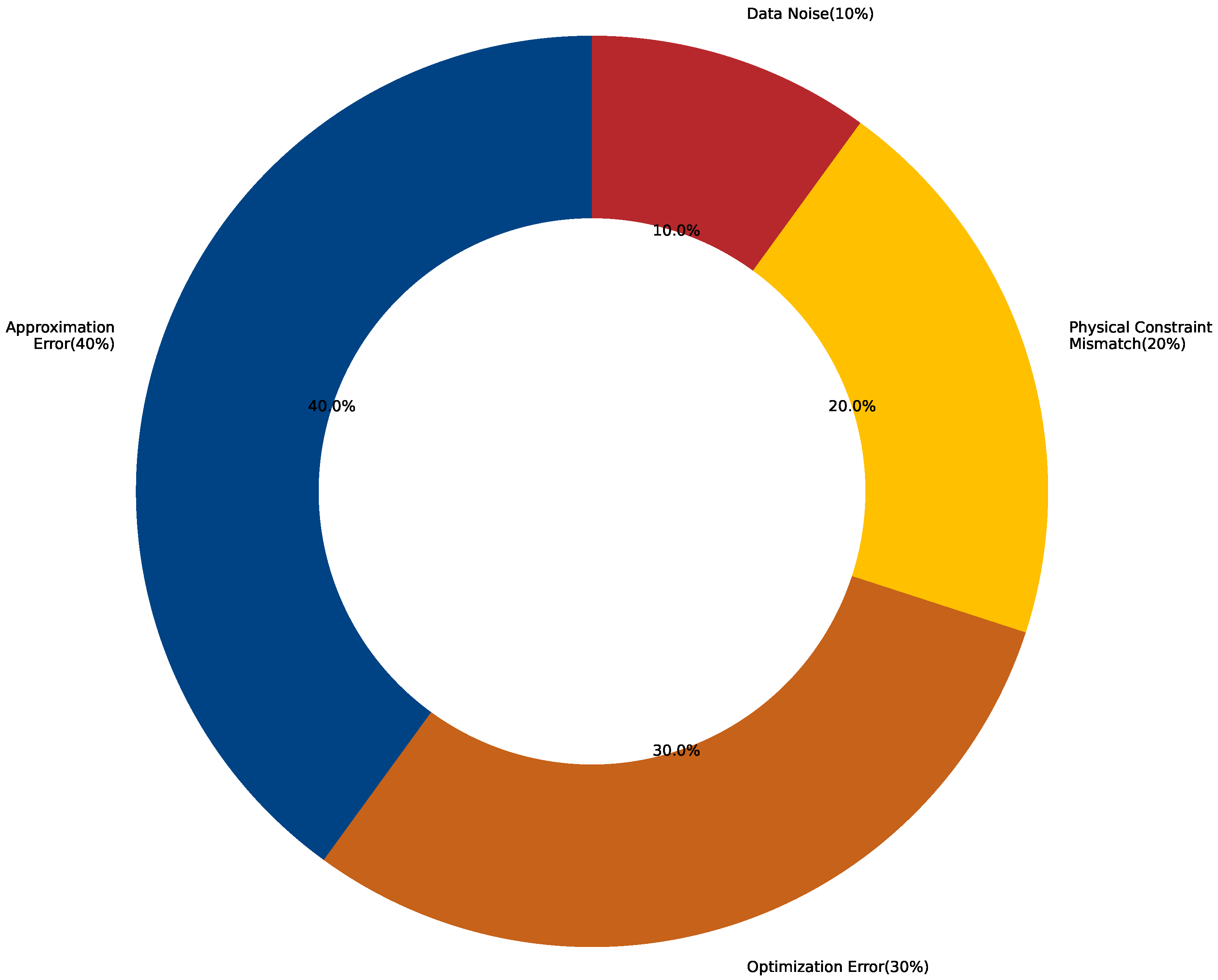
- Approximation Error (40%) arises due to the limitations in the neural network’s representational capacity. Despite its capability, the network may not fully capture the complexity of the underlying physical problem, leading to an inherent error in approximating the target function. This error can be mitigated by improving the network architecture, such as increasing the depth or width of the network.
- Optimization Error (30%) originates from the suboptimal convergence during the training process. Even with a sufficient model capacity, the optimization algorithm, including factors such as learning rate and initialization, might not converge to the global optimum, leading to a non-ideal solution. This error can be reduced through better optimization strategies and fine-tuning hyperparameters.
- Physical Constraint Mismatch (20%) refers to the error caused by inaccuracies in the representation of the physical constraints (e.g., partial differential equations, boundary conditions) within the model. If the constraints are not accurately modeled or do not fully reflect the actual physical system, a mismatch arises. Addressing this error typically involves refining the physical model or more accurately incorporating the constraints into the network’s loss function.
- Data Noise (10%) represents the uncertainty or noise inherent in real-world data. Experimental data often contain noise due to measurement errors, which can lead to discrepancies between the network’s predictions and the observed values. Reducing this error may involve improving data quality or applying noise filtering techniques.
4. Interdisciplinary Applications
4.1. Computational Physics and Engineering
4.2. Biomedical Systems
4.3. Earth and Environmental Science
5. Emerging Paradigms and Future Directions
5.1. Neuro-Symbolic Integration
5.2. Federated Physics Learning
5.3. Quantum-Enhanced Architectures
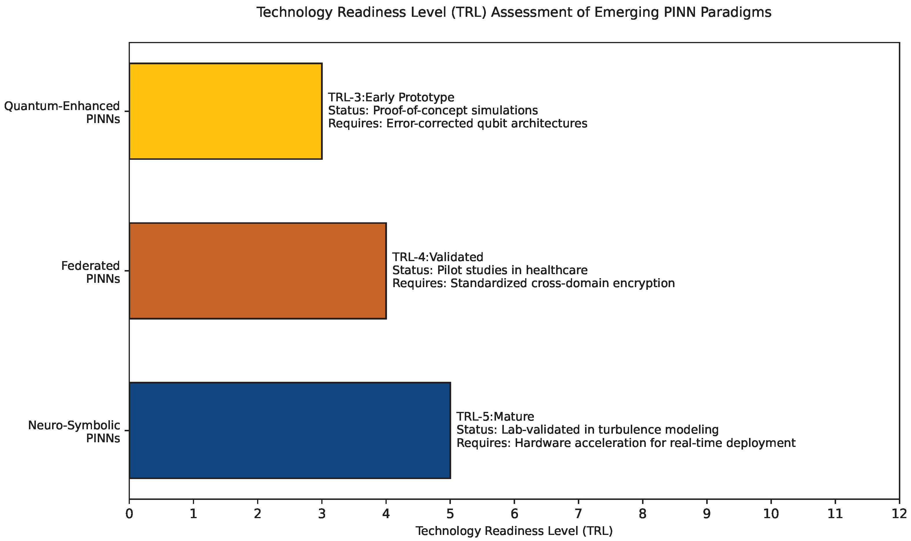
- Neuro-symbolic PINNs (TRL-5): Laboratory validation in turbulence/closures; requires hardware acceleration for real-time deployment.
- Federated PINNs (TRL-4): Pilot studies in healthcare; needs standardization of cross-domain encryption protocols.
- Quantum-PINNs (TRL-3): Proof-of-concept simulations; dependent on error-corrected qubit architectures.
6. Conclusions
6.1. Key Contributions
6.2. Current Challenges
6.3. Strategic Roadmap
Author Contributions
Funding
Data Availability Statement
Conflicts of Interest
Glossary
| FEM | Finite Element Method |
| MRI | Magnetic Resonance Imaging |
| PINN | Physics-Informed Neural Networks |
| PDE | Partial Differential Equations |
| FVM | Finite Volume Method |
| FDM | Finite Difference Method |
| CNN | Convolutional Neural Networks |
| SSIM | Structural Similarity |
| MLP | Multilayer Perceptron |
| NTK | Neural Tangent Kernel |
| LSTM | Long Short-Term Memory |
| LES | Large Eddy Simulation |
| MSE | Mean Square Error |
| TRL | Technology Readiness Level |
| XPINN | Extended Physics-Informed Neural Networks |
| VPINN | Variational Physics-Informed Neural Networks |
| HFD-PINN | High-Fidelity Data-Driven PINNs |
| TFE-PINN | Turbulence-Focused Enhanced PINNs |
| MC-PINN | Multiscale Climate PINNs |
| Fed-PINN | Federated PINNs |
References
- Strang, G.; Fix, G.J.; Griffin, D. An Analysis of the Finite-Element Method; Prentice-Hall: Hoboken, NJ, USA, 1974. [Google Scholar]
- John, D.; Anderson, J. Computational Fluid Dynamics: The Basics with Applications; Mechanical Engineering Series; McGraw-Hill: New York, NY, USA, 1995; pp. 261–262. [Google Scholar]
- Versteeg, H.; Malalasekera, W. Computational Fluid Dynamics; The Finite Volume Method; McGraw-Hill: New York, NY, USA, 1995; pp. 1–26. [Google Scholar]
- Quarteroni, A.; Valli, A. Domain Decom Position Methods for Partial Differential Equations; Oxford University Press: Oxford, UK, 1999. [Google Scholar]
- Hughes, T.J.; Cottrell, J.A.; Bazilevs, Y. Isogeometric analysis: CAD, finite elements, NURBS, exact geometry and mesh refinement. Comput. Methods Appl. Mech. Eng. 2005, 194, 4135–4195. [Google Scholar] [CrossRef]
- Goodfellow, I.; Bengio, Y.; Courville, A.; Bengio, Y. Deep Learning; MIT Press Cambridge: Cambridge, MA, USA, 2016; Volume 1. [Google Scholar]
- Raissi, M.; Perdikaris, P.; Karniadakis, G. Physics-informed neural networks: A deep learning framework for solving forward and inverse problems involving nonlinear partial differential equations. J. Comput. Phys. 2019, 378, 686–707. [Google Scholar] [CrossRef]
- Karniadakis, G.E.; Kevrekidis, I.G.; Lu, L.; Perdikaris, P.; Wang, S.; Yang, L. Physics-informed machine learning. Nat. Rev. Phys. 2021, 3, 422–440. [Google Scholar] [CrossRef]
- Lawal, Z.K.; Yassin, H.; Lai, D.T.C.; Che Idris, A. Physics-informed neural network (PINN) evolution and beyond: A systematic literature review and bibliometric analysis. Big Data Cogn. Comput. 2022, 6, 140. [Google Scholar] [CrossRef]
- Huang, B.; Wang, J. Applications of physics-informed neural networks in power systems-a review. IEEE Trans. Power Syst. 2022, 38, 572–588. [Google Scholar] [CrossRef]
- Lu, L.; Meng, X.; Mao, Z.; Karniadakis, G.E. DeepXDE: A deep learning library for solving differential equations. SIAM Rev. 2021, 63, 208–228. [Google Scholar] [CrossRef]
- Wang, S.; Li, B.; Chen, Y.; Perdikaris, P. Piratenets: Physics-informed deep learning with residual adaptive networks. J. Mach. Learn. Res. 2024, 25, 1–51. [Google Scholar]
- Shin, Y.; Darbon, J.; Karniadakis, G.E. On the convergence of physics informed neural networks for linear second-order elliptic and parabolic type PDEs. arXiv 2020, arXiv:2004.01806. [Google Scholar]
- Cai, S.; Mao, Z.; Wang, Z.; Yin, M.; Karniadakis, G.E. Physics-informed neural networks (PINNs) for fluid mechanics: A review. Acta Mech. Sin. 2021, 37, 1727–1738. [Google Scholar] [CrossRef]
- Kim, D.; Lee, J. A review of physics informed neural networks for multiscale analysis and inverse problems. Multiscale Sci. Eng. 2024, 6, 1–11. [Google Scholar] [CrossRef]
- Research, I. Quantum-Enhanced PINN for Electronic Structure Calculations; Technical Report, IBM Technical Report; IBM: Armonk, NY, USA, 2025. [Google Scholar]
- Li, X.; Wang, H. Privacy-preserving Federated PINNs for Medical Image Reconstruction. Med. Image Anal. 2025, 88, 101203. [Google Scholar]
- Ceccarelli, D. Bayesian Physics-Informed Neural Networks for Inverse Uncertainty Quantification Problems in Cardiac Electrophysiology. 2019. Available online: https://www.politesi.polimi.it/handle/10589/175559 (accessed on 10 July 2025).
- Cuomo, S.; Di Cola, V.S.; Giampaolo, F.; Rozza, G.; Raissi, M.; Piccialli, F. Scientific machine learning through physics–informed neural networks: Where we are and what’s next. J. Sci. Comput. 2022, 92, 88. [Google Scholar] [CrossRef]
- Chen, G.; Yu, B.; Karniadakis, G. SyCo-PINN: Symbolic-Neural Collaboration for PDE Discovery. In Proceedings of the AAAI Conference on Artificial Intelligence, Philadelphia, PA, USA, 25 February–4 March 2025; pp. 12345–12353. [Google Scholar]
- Jagtap, A.D.; Kawaguchi, K.; Karniadakis, G.E. Adaptive activation functions accelerate convergence in deep and physics-informed neural networks. J. Comput. Phys. 2020, 404, 109136. [Google Scholar] [CrossRef]
- Jagtap, A.D.; Kharazmi, E.; Karniadakis, G.E. Conservative physics-informed neural networks on discrete domains for conservation laws: Applications to forward and inverse problems. Comput. Methods Appl. Mech. Eng. 2020, 365, 113028. [Google Scholar] [CrossRef]
- Dwivedi, V.; Parashar, N.; Srinivasan, B. Distributed physics informed neural network for data-efficient solution to partial differential equations. arXiv 2019, arXiv:1907.08967. [Google Scholar]
- Liu, H.; Zhang, Y.; Wang, L. Pre-training physics-informed neural network with mixed sampling and its application in high-dimensional systems. J. Syst. Sci. Complex. 2024, 37, 494–510. [Google Scholar] [CrossRef]
- Wang, S.; Teng, Y.; Perdikaris, P. Understanding and mitigating gradient flow pathologies in physics-informed neural networks. SIAM J. Sci. Comput. 2021, 43, A3055–A3081. [Google Scholar] [CrossRef]
- Jagtap, A.D.; Karniadakis, G.E. Extended physics-informed neural networks (XPINNs): A generalized space-time domain decomposition based deep learning framework for nonlinear partial differential equations. Commun. Comput. Phys. 2020, 28, 2002–2041. [Google Scholar] [CrossRef]
- De Ryck, T.; Mishra, S. Error analysis for physics-informed neural networks (PINNs) approximating Kolmogorov PDEs. Adv. Comput. Math. 2022, 48, 79. [Google Scholar] [CrossRef]
- Yu, J.; Lu, L.; Meng, X.; Karniadakis, G.E. Gradient-enhanced physics-informed neural networks for forward and inverse PDE problems. Comput. Methods Appl. Mech. Eng. 2022, 393, 114823. [Google Scholar] [CrossRef]
- Liu, J.; Chen, X.; Sun, H. Adaptive deep learning for time-dependent partial differential equations. J. Comput. Phys. 2022, 463, 111292. [Google Scholar]
- Zhang, X.; Tu, C.; Yan, Y. Physics-informed neural network simulation of conjugate heat transfer in manifold microchannel heat sinks for high-power IGBT cooling. Int. Commun. Heat Mass Transf. 2024, 159, 108036. [Google Scholar] [CrossRef]
- Kharazmi, E.; Zhang, Z.; Karniadakis, G.E. hp-VPINNs: Variational physics-informed neural networks with domain decomposition. Comput. Methods Appl. Mech. Eng. 2021, 374, 113547. [Google Scholar] [CrossRef]
- Xiang, Z.; Peng, W.; Zhou, W.; Yao, W. Hybrid finite difference with the physics-informed neural network for solving PDE in complex geometries. arXiv 2022, arXiv:2202.07926. [Google Scholar] [CrossRef]
- Berrone, S.; Canuto, C.; Pintore, M. Variational physics informed neural networks: The role of quadratures and test functions. J. Sci. Comput. 2022, 92, 100. [Google Scholar] [CrossRef]
- Bai, X.D.; Wang, Y.; Zhang, W. Applying physics informed neural network for flow data assimilation. J. Hydrodyn. 2020, 32, 1050–1058. [Google Scholar] [CrossRef]
- Schwab, C.; Zech, J. Deep Learning in High Dimension: Neural Network Expression Rates for Analytic Functions. SAM Res. Rep. 2021, 2021. [Google Scholar]
- Wang, S.; Zhang, L.; Li, X. Convergence Analysis of Nonlinear PDEs Solved by Physics-Informed Neural Networks with Pseudo-Linearization. arXiv 2023, arXiv:2311.00234. [Google Scholar]
- Chen, X.; Zhang, Y.; Li, M. Information bottleneck with physical constraints for enhancing generalization in partial differential equations. J. Comput. Phys. 2023, 461, 111–128. [Google Scholar]
- Yang, Z.; Zhang, X.; Li, Y. Micropinn: A physics-informed neural network for crystal plasticity simulation. J. Comput. Mater. Sci. 2023, 207, 110179. [Google Scholar]
- Zhang, S.; Zhang, C.; Han, X.; Wang, B. MRF-PINN: A multi-receptive-field convolutional physics-informed neural network for solving partial differential equations. Comput. Mech. 2025, 75, 1137–1163. [Google Scholar] [CrossRef]
- Trahan, C.; Loveland, M.; Dent, S. Quantum Physics-Informed Neural Networks. Entropy 2024, 26, 649. [Google Scholar] [CrossRef] [PubMed]

| Architecture | NN Layers | Activation | Data Generation | Distinctive Feature |
|---|---|---|---|---|
| VPINN | 4–8 Dense | Tanh/Legendre | Sobol Sequence | Variational Residual Form |
| XPINN | 3–5 Subnets | Swish | Adaptive RAR | Domain Decomposition |
| HFD-PINN | 6–10 CNN-MLP | ReLU | Physics-Initiated | Hybrid Finite-Difference |
| TFE-PINN | 7–12 LSTM-MLP | GELU | LES Data Assimilation | Turbulence Closure Modeling |
| Module | Function | Implementation | Performance Gain |
|---|---|---|---|
| Residual Connections | Mitigate gradient pathology | DenseNet [11] | faster convergence |
| Adaptive Activation | Enhance nonlinear expressivity | Learnable Tanh [21] | accuracy boost |
| Mixed-Precision Training | Accelerate tensor operations | FP16-FP32 hybrid [24] | memory reduction |
| Dynamic Weighting | Balance multi-physics constraints | NTK theory [25] | success rate improvement |
| Domain Decomposition | Enable high-dimensional solutions | XPINN [26] | 5× speedup in 3D turbulence |
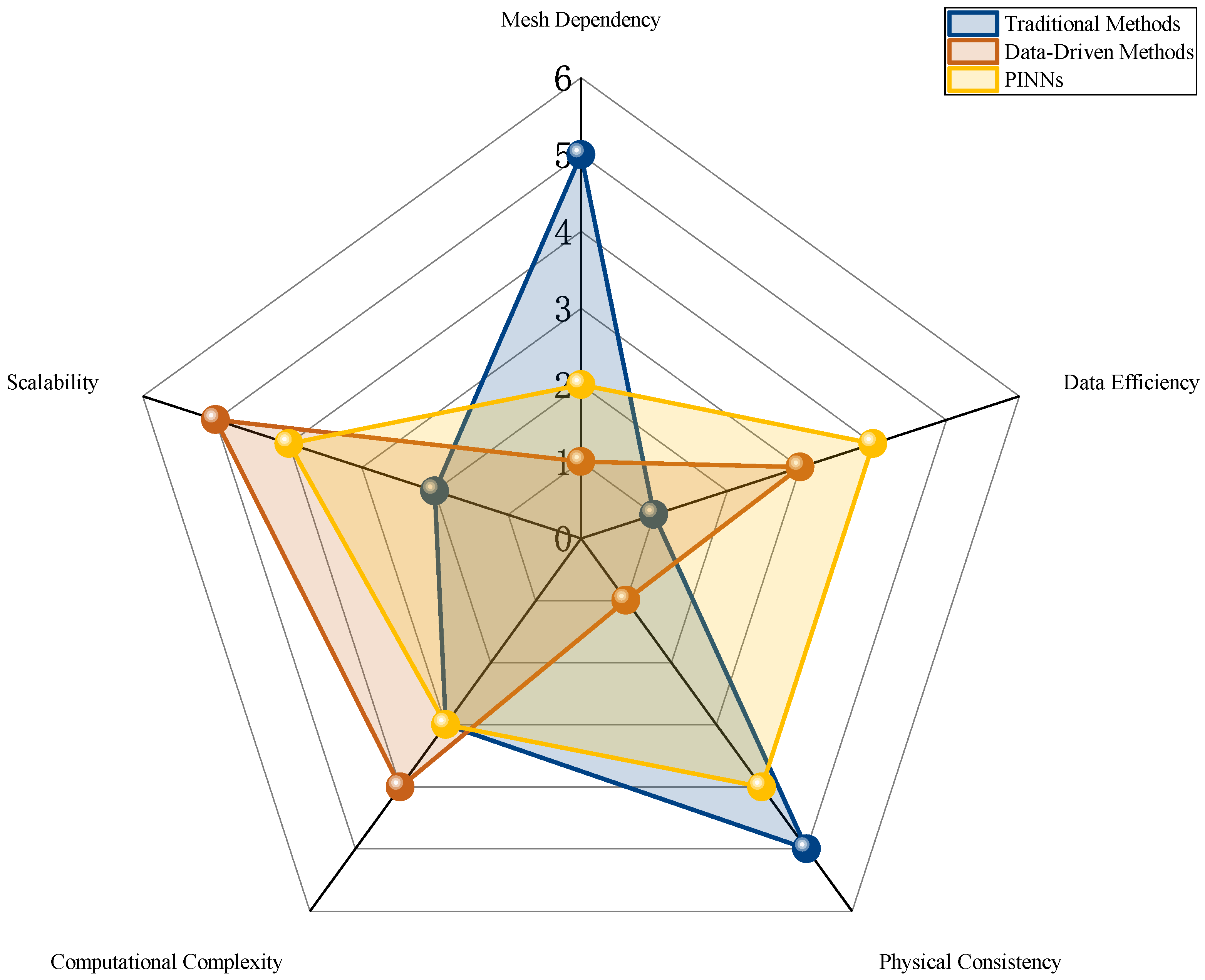
| Method | Computational Efficiency | Data Efficiency | Physical | Training | Reference |
|---|---|---|---|---|---|
| (vs. FEM) | (vs. CNN) | Consistency (1–5) | Time (h) | ||
| VPINN | 60% less data | 4.7 | 1.2 | [33] | |
| HFD-PINN | 80% less data | 4.2 | 0.8 | [32] | |
| XPINN | 70% less data | 4.5 | 3.5 | [26] | |
| FEM (Baseline) | N/A | 5.0 | 5.1 | [34] | |
| CNN (Baseline) | 2.1 | 4.3 | [6] |
| Application | Method | Error Reduction | Compute Time | Reference |
|---|---|---|---|---|
| Turbulence Modeling | TFE-PINN vs. LES | 62% | 14 h vs. 72 h | [30] |
| MRI Reconstruction | ReconPINN vs. CS | SSIM + 0.18 | 2 min vs. 15 min | [15] |
| Climate Prediction | MC-PINN vs. CMIP6 | 37% | 18 h vs. 100 h | [39] |
| Seismic Localization | SeisPINN vs. Traditional | 76% | 5 s vs. 30 s | [20] |
Disclaimer/Publisher’s Note: The statements, opinions and data contained in all publications are solely those of the individual author(s) and contributor(s) and not of MDPI and/or the editor(s). MDPI and/or the editor(s) disclaim responsibility for any injury to people or property resulting from any ideas, methods, instructions or products referred to in the content. |
© 2025 by the authors. Licensee MDPI, Basel, Switzerland. This article is an open access article distributed under the terms and conditions of the Creative Commons Attribution (CC BY) license (https://creativecommons.org/licenses/by/4.0/).
Share and Cite
Ren, Z.; Zhou, S.; Liu, D.; Liu, Q. Physics-Informed Neural Networks: A Review of Methodological Evolution, Theoretical Foundations, and Interdisciplinary Frontiers Toward Next-Generation Scientific Computing. Appl. Sci. 2025, 15, 8092. https://doi.org/10.3390/app15148092
Ren Z, Zhou S, Liu D, Liu Q. Physics-Informed Neural Networks: A Review of Methodological Evolution, Theoretical Foundations, and Interdisciplinary Frontiers Toward Next-Generation Scientific Computing. Applied Sciences. 2025; 15(14):8092. https://doi.org/10.3390/app15148092
Chicago/Turabian StyleRen, Zhiyuan, Shijie Zhou, Dong Liu, and Qihe Liu. 2025. "Physics-Informed Neural Networks: A Review of Methodological Evolution, Theoretical Foundations, and Interdisciplinary Frontiers Toward Next-Generation Scientific Computing" Applied Sciences 15, no. 14: 8092. https://doi.org/10.3390/app15148092
APA StyleRen, Z., Zhou, S., Liu, D., & Liu, Q. (2025). Physics-Informed Neural Networks: A Review of Methodological Evolution, Theoretical Foundations, and Interdisciplinary Frontiers Toward Next-Generation Scientific Computing. Applied Sciences, 15(14), 8092. https://doi.org/10.3390/app15148092