An Empirical Comparison of Urban Road Travel Time Prediction Methods—Deep Learning, Ensemble Strategies and Performance Evaluation

Abstract

Urban road travel time prediction is a critical component of intelligent transportation systems. However, accurate prediction remains challenging due to the high volatility and randomness of urban road traffic. This study compares the predictive performance of deep learning methods with traditional shallow learning methods for urban road travel time prediction, and explores the potential for improving prediction effectiveness through multi-run training strategies for hyperparameter optimization and ensemble learning. The study employs urban road travel time data from Shenzhen, China, designing 10 prediction scenarios with different sliding time window lengths and prediction scales. To address the randomness issue in deep learning models, we adopt a strategy of conducting five independent training runs for each hyperparameter configuration and using statistical measures to obtain stable performance evaluations. For model comparison, we implement multiple shallow learning models (linear regression, ridge regression, LASSO regression, random forest) and deep learning models (LSTM-DNN, DNN), and construct ensemble learning models based on linear regression and LSTM-DNN as base learners. The experimental results demonstrate that: (1) deep learning models generally outperform shallow learning models in terms of Mean Absolute Percentage Error (MAPE), particularly the LSTM-DNN model which achieves the best MAPE values across all prediction scenarios with 30 min sliding time windows; (2) in terms of Root Mean Square Error (RMSE), shallow learning models such as random forest perform better in most scenarios; (3) ensemble learning models show certain advantages in some prediction scenarios, but the improvement effects are limited and scenario-dependent. The research results provide empirical reference for method selection in urban road travel time prediction, while also revealing the limitations of single data sources and the differences in model performance under different evaluation metrics, offering directions for future research.

1. Introduction

1.1. Research Background

Urban road travel time prediction, as a key component of intelligent transportation systems, plays an increasingly important role in modern urban management and travel planning. With the acceleration of global urbanization, traffic congestion has become a universal challenge constraining sustainable urban development, making accurate and reliable travel time prediction particularly critical.

Problem-oriented challenges: Urban road travel time prediction faces multiple technical challenges. First, urban road networks are significantly more complex than highway systems, containing numerous intersections, traffic signal controls, and interwoven different types of roads. Signal-controlled intersections cause urban road traffic to exhibit typical interrupted flow characteristics, leading to periodic fluctuations in travel times. Second, urban road traffic demand exhibits high dynamism and uncertainty, influenced by numerous factors such as weekday patterns, seasonal variations, and special events. Furthermore, random events such as traffic accidents, road construction, and adverse weather conditions occur frequently, further increasing the uncertainty of travel times. Traditional prediction methods show obvious limitations when addressing these complexities. Statistical models often struggle to capture nonlinear relationships and multi-variable interactions; shallow learning methods poorly handle sudden events; single models are prone to overfitting or underfitting specific traffic patterns. These challenges have generated demand for more advanced prediction methods, particularly those that can integrate the advantages of deep learning while overcoming its inherent randomness.

Demand-driven requirements: Multiple practical needs further highlight the importance of precise travel time prediction. For traffic management authorities, accurate travel time prediction serves as the foundation for achieving intelligent signal control, dynamic route planning, and emergency resource allocation, helping to alleviate traffic congestion and improve overall road network efficiency. Traffic planners require reliable prediction tools to evaluate the potential impacts of different policy measures and infrastructure investments. From travelers’ perspectives, accurate travel time prediction directly affects travel decisions and route choices. Compared to simple historical averages or static estimates, dynamic and reliable prediction information helps travelers make more reasonable plans, reducing unnecessary waiting and detours, and improving travel experience and efficiency. In commercial applications, precise travel time prediction is crucial for logistics delivery, ride-hailing dispatch, and shared mobility services. These sectors rely on high-quality travel time predictions to optimize vehicle scheduling, route planning, and resource allocation, directly impacting operational costs and service quality.

Given the aforementioned problems and requirements, this study focuses on a key question: how to construct more accurate and stable urban road travel time prediction models. Traditional methods and single deep learning models each have limitations, while the multi-run training and ensemble learning prediction framework proposed in this study aims to combine the advantages of both while overcoming their respective shortcomings. Specifically, the multi-run training method in this study provides a systematic solution to the randomness problem in deep learning model training, while the ensemble learning framework improves prediction stability and accuracy by integrating the advantages of multiple models. This study not only advances methodological innovation in the traffic prediction field theoretically, but also provides technical support for building more intelligent and reliable urban traffic management systems in practice, ultimately contributing to alleviating urban traffic congestion, enhancing citizen travel experience, and promoting sustainable urban development.

1.2. Problems and Challenges

Specifically, urban road travel time prediction faces the following important challenges:

(1) Intersection signal control timing: Unlike highways, urban roads contain intersections of different scales on arterials, collectors, and local roads. Signal-controlled intersections cause vehicles operating in the road network to form interrupted flow rather than continuous flow, resulting in periodic fluctuations in average segment speeds, thereby exacerbating the volatility of segment travel times. This characteristic makes urban road travel time prediction more complex compared to highways.

(2) Dynamism and uncertainty of traffic demand: Highway traffic demand exhibits relatively stable changes with strong periodicity. However, urban road segment traffic demand is highly dynamic with intense variation. Although periodicity exists, it appears less obvious than highways due to strong volatility, significantly increasing the randomness of segment average speed changes and consequently the randomness of segment travel time variations.

(3) Traffic incident impacts: Compared to highways, urban road traffic conditions are more susceptible to various traffic incidents, particularly non-recurrent traffic events. Recurrent traffic events mainly include rush hour traffic congestion, while non-recurrent traffic events primarily include traffic accidents, construction, and weather changes. If occasional mobile bottlenecks or different types of traffic conflicts (such as vehicle–vehicle conflicts, vehicle–bicycle conflicts, and vehicle–pedestrian conflicts) are also considered as traffic events, it can be understood that non-recurrent traffic events affecting traffic conditions in urban roads have diverse sources, strong randomness, varied development trends, and different impact ranges, causing urban road segments and networks to experience sudden traffic congestion spanning different spatial and temporal distances due to the occurrence of multiple non-recurrent traffic events.

(4) Randomness problem in prediction models: In deep learning models, particularly recurrent neural networks such as long short-term memory (LSTM) networks, there exists a randomness problem—even when using the same network structure and hyperparameters, different prediction results may be produced in different training iterations. This randomness stems from random weight initialization and randomness in the optimization process, increasing the difficulty of model selection and evaluation.

1.3. Research Objectives and Innovations

This study develops deep learning-based urban road travel time prediction models and methods, and compares representative shallow learning models and methods from existing research from multiple perspectives including accuracy and stability, analyzing the applicability and characteristics of deep learning models and methods in the field of urban road travel time prediction.

The main innovations of this study include the following:

(1) A multi-run training method for hyperparameter optimization: To address the randomness problem in deep learning models, we propose a multi-run training method for hyperparameter optimization of long short-term memory with deep neural network (LSTM-DNN) deep learning models. This method trains multiple model instances for each hyperparameter configuration and evaluates the collective performance of each configuration based on statistical measures (such as median and standard deviation) to select the optimal hyperparameter configuration. This method effectively solves the randomness problem in deep learning model training, making model selection more reliable.

(2) Ensemble learning prediction framework: We propose an ensemble learning framework suitable for urban road travel time prediction that integrates shallow learning and deep learning models to improve prediction performance. This framework selects base learners with different characteristics (such as linear regression and LSTM-DNN models) and combines their prediction results through various meta-learners (such as linear regression, random forest, LSTM-DNN, and DNN models), achieving improved prediction performance.

(3) Comprehensive empirical research: Based on actual urban road travel time data from Shenzhen, China, extensive experiments were conducted comparing the performance of different models under various prediction scenarios. The research results provide valuable empirical reference for the field of urban road travel time prediction.

1.4. Manuscript Structure

The structure of the remainder of this manuscript is organized as follows: Section 2 reviews related work on travel time prediction methods, including traditional methods, deep learning applications, and ensemble learning in traffic prediction; Section 3 details our proposed methodology, including the sliding time window-based short-term dynamic prediction mechanism and ensemble learning model design; Section 4 describes the experimental setup and analyzes the results, comparing the performance of different models in detail; Section 5 discusses additional details and implications of the results; Section 6 summarizes the research findings and discusses future research directions.

2. Literature Review

2.1. Traditional Travel Time Prediction Methods

Traditional travel time prediction methods are primarily based on statistics and classical machine learning theory. Ahmed and Cook [1] first applied Box–Jenkins time series analysis techniques to highway traffic flow and occupancy prediction in 1979, establishing the theoretical foundation for autoregressive integrated moving average (ARIMA) models. Their study analyzed 166 datasets from three monitoring systems in Los Angeles, Minneapolis, and Detroit, finding that the ARIMA (0, 1, 3) model was more accurate than traditional methods such as moving averages and double exponential smoothing in representing highway time-series data.

Building upon this foundation, Kamarianakis and Prastacos [2] compared the performance of univariate ARIMA, vector autoregressive moving average (VARMA), and spatiotemporal ARIMA (STARIMA) models in urban road network traffic flow prediction. Using data from 25 loop detectors in Athens, Greece, they found that ARIMA, VARMA, and STARIMA models had comparable prediction performance, while historical average models could not cope with data variability. Billings and Yang [3] further applied ARIMA models to urban road travel time prediction, validating the potential and effectiveness of ARIMA modeling in travel time prediction through a case study of Minnesota State Highway 194.

In addition to time-series methods, machine learning techniques have been widely applied to travel time prediction. Wu et al. [4] first applied support vector regression (SVR) to travel time prediction, comparing it with other benchmark prediction methods using real highway traffic data. The results showed that SVR predictors could significantly reduce the relative mean error and Root Mean Square Error of predicted travel times. Yang et al. [5] proposed a short-term traffic flow prediction model based on support vector machines (SVM). Compared with BP neural network prediction models, they found that this model was superior to BP neural network models in terms of prediction accuracy, convergence time, generalization ability, and optimization potential.

With the development of ensemble learning theory, tree-based ensemble methods began to receive attention. Li and Bai [6] used gradient boosting regression trees (GBRT) to analyze and model freight vehicle travel time prediction, utilizing Bayesian optimization for model fitting. Results showed that both pre-departure and post-departure prediction accuracies exceeded 80%. Cai et al. [7] proposed an improved k-nearest neighbor (KNN) model based on spatiotemporal correlation, replacing equivalent distances with physical distances and using Gaussian-weighted Euclidean distance to select nearest neighbors. Experimental results showed that the improved KNN model was more suitable for short-term traffic multi-step prediction than other models.

Van Lint et al. [8] proposed a highway travel time prediction framework based on state-space neural networks (SSNN), which exhibited both accuracy and robustness to missing or corrupted input data. Although the SSNN model is a neural network, its design is based on highway segment layout, combining the generality of neural network approaches with traffic-related “white-box” design.

Although traditional methods have achieved certain success in travel time prediction, these methods still have obvious limitations when dealing with urban road travel time prediction. First, statistical models such as ARIMA require data to be stationary or stationary after differencing, while urban road travel time data are often highly non-stationary. Second, shallow machine learning methods struggle to effectively capture complex nonlinear relationships and multi-level features in traffic data. Finally, these methods have poor adaptability to sudden traffic events and cannot accurately model the impact of non-recurrent events such as traffic accidents and construction on travel times.

2.2. Applications of Deep Learning Methods in Travel Time Prediction

The rise of deep learning technology has brought new opportunities to the field of traffic prediction. Huang et al. [9] applied deep learning methods to traffic research in 2014, proposing a deep architecture consisting of deep belief networks (DBN) and multi-task regression layers for traffic flow prediction. This study used DBN for unsupervised feature learning and multi-task regression at the top layer for supervised prediction. Experimental results showed that this method improved performance by approximately 5% compared to state-of-the-art methods.

With the development of recurrent neural network technology, Tian and Pan [10] proposed a short-term traffic flow prediction model based on long short-term memory recurrent neural networks (LSTM RNN). This model utilized three multiplicative units in memory blocks to dynamically determine optimal time lags, overcoming the limitation of traditional models that require predefined input historical data lengths. Compared with models such as random walk (RW), support vector machines (SVM), feedforward neural networks (FFNN), and stacked autoencoders (SAE), the LSTM RNN model demonstrated higher accuracy and generalization capability.

Lv et al. [11] proposed a deep learning traffic flow prediction method based on stacked autoencoders that considered spatial and temporal correlations, using stacked autoencoders to learn generic traffic flow features and training in a greedy layer-wise manner. Experiments showed that this method had superior performance in traffic flow prediction. Ma et al. [12] pioneered a convolutional neural network (CNN)-based approach, treating traffic learning as image processing by converting spatiotemporal traffic dynamics into images describing temporal and spatial relationships of traffic flow through two-dimensional spatiotemporal matrices. Experimental results on real traffic networks in Beijing showed that this method improved average accuracy by 42.91% compared to other algorithms.

Fu et al. [13] compared traffic flow prediction models based on LSTM networks and gated recurrent units (GRU). Experimental results showed that RNN-based deep learning methods such as LSTM and GRU outperformed ARIMA models in performance. Wang et al. [14] proposed a deep learning method based on error-feedback recurrent convolutional neural network (eRCNN) structure, integrating spatiotemporal traffic speeds of continuous road segments as input matrices and explicitly utilizing implicit correlations between nearby segments to improve prediction accuracy.

For the specific needs of travel time prediction, Liu et al. [15] established a series of long short-term memory neural networks with deep neural layer (LSTM-DNN) combination models using 16 hyperparameter settings and conducted detailed performance investigations on a 90-day travel time dataset from the Caltrans Performance Measurement System (PeMS). This study found that different hyperparameter settings caused deep learning models to exhibit different characteristics, providing important insights for model structure optimization.

Polson and Sokolov [16] developed a deep learning architecture combining L1 regularized linear models and a sequence of tanh layers for traffic flow prediction. The main contribution of this study was developing an architecture capable of capturing sharp nonlinearities due to transitions between free flow, breakdown, recovery, and congestion. Sun and Kim [17] proposed two deep learning models based on LSTM neural networks and self-attention mechanisms—hybrid LSTM and sequential LSTM—for jointly predicting next location and travel time.

Ma et al. [18] addressed the bus travel time prediction problem by proposing a novel segment-based approach that combines real-time taxi and bus datasets, capable of automatically dividing bus routes into dwelling and transit segments. Wang et al. [19] proposed an end-to-end deep learning travel time estimation framework called DeepTTE, which captures spatial correlations through geo-convolution operations that integrate geographical information into classical convolutions, while capturing temporal dependencies by stacking recurrent units on geo-convolutional layers.

In recent years, more advanced deep learning architectures have been proposed. Ke et al. [20] proposed the Fusion Convolutional Long Short-Term Memory Network (FCL-Net), which addresses spatial dependencies, temporal dependencies, and exogenous dependencies simultaneously by stacking and fusing multiple convolutional LSTM layers, standard LSTM layers, and convolutional layers. Abdollahi et al. [21] proposed a multi-step deep learning algorithm for travel time prediction that starts with data preprocessing, then enhances data by incorporating external datasets, and applies extensive feature learning and engineering.

Wu et al. [22] proposed a deep neural network-based traffic flow prediction model (DNN-BTF) that fully utilizes weekly/daily periodicity and spatiotemporal characteristics of traffic flow, introducing an attention-based model that automatically learns to determine the importance of past traffic flow. Du et al. [23] proposed a Deep Irregular Convolutional Residual LSTM network model (DST-ICRL) for urban traffic passenger flow prediction, which models passenger flows between different transportation lines as multi-channel matrices analogous to image RGB pixel matrices.

Recent studies also include the Bi-Directional Isometric Gated Recurrent Unit (BDIGRU) proposed by Chen et al. [24], the Spatial-Temporal Attention Neural Network (STANN) for deep learning traffic flow prediction proposed by Do et al. [25], and the Short-Term and Long-Term Integrated Transformer (SLIT) proposed by Lin et al. [26]. Liu et al. [27] proposed a GraphSAGE-based Dynamic Spatial-Temporal Graph Convolutional Network (DST-GraphSAGE), and Sheng et al. [28] proposed a deep spatial-temporal travel time prediction model based on trajectory features.

Jang’s [29] recent study compared the performance of three machine learning algorithms—k-nearest neighbors (k-NN), LSTM, and transformer—in travel time prediction, with results showing that transformer achieved the lowest prediction error (10.3%). Afandizadeh et al. [30] conducted a comprehensive review of the applications of deep learning algorithms and classical models in traffic prediction, reviewing 111 important research works since the 1980s.

Although deep learning methods have demonstrated powerful capabilities in travel time prediction, challenges remain: high training costs, difficult hyperparameter optimization, randomness issues, and poor interpretability. Particularly, the randomness problem in deep learning models—even when using the same network structure and hyperparameters, different prediction results may be produced in different training iterations—increases the difficulty of model selection and evaluation.

While our literature review has identified these emerging architectures, this study focuses on establishing a systematic comparison framework using well-established deep learning methods (LSTM-DNN) alongside traditional shallow learning approaches. This methodological choice allows us to address the critical randomness issues in deep learning model training and develop robust ensemble strategies. The comprehensive evaluation framework established in this study provides a solid foundation for future incorporation of transformer-based and graph neural network approaches when appropriate datasets and computational resources become available.

2.3. Applications of Ensemble Learning in Traffic Prediction

Ensemble learning completes machine learning tasks by constructing multiple base learners and combining their training results, theoretically achieving significantly superior generalization capability compared to single learners. Zhang and Haghani [31] employed gradient boosting methods to improve travel time prediction. Results showed that tree-based ensemble methods, by combining simple regression trees with “poor” performance, typically produce high prediction accuracy. Compared to other machine learning methods treated as black boxes, tree-based ensemble methods provide interpretable results while requiring less data preprocessing, being able to handle different types of predictor variables, and fitting complex nonlinear relationships.

Wang et al. [32] proposed a new Bayesian combination method for short-term traffic flow prediction, combining ARIMA models, Kalman filtering, and BP neural networks. The main improvement of this method was changing from considering the entire model prediction values to considering only model prediction values within the sliding time window, making the combination model more sensitive to the perturbation performance of component predictors and able to adjust its weights more rapidly. Zheng et al. [33] proposed a Bayesian combination neural network method for short-term highway traffic flow prediction. This method introduced a neural network model that combined predictions from individual neural network predictors according to an adaptive heuristic credit assignment algorithm based on conditional probability theory and Bayes’ rule.

Yin et al. [34] proposed a bus travel time prediction interval model based on road segment sharing, multiple routes’ driving style similarity, and the bootstrap method. The model first divides the predicted route into segments, partitioning adjacent stations shared by multiple routes into one segment, then uses hierarchical clustering algorithms to group all drivers of multiple bus routes in that segment according to driving style, and finally uses the bootstrap method to construct bus travel time prediction intervals for different categories of drivers. Zhu et al. [35] proposed a multiple-factor based sparse urban travel time prediction method, designing a three-layer artificial neural network model that fuses multiple factors from large-scale probe vehicle data to estimate travel time. The study incorporated different factors to examine their influence on link travel time and validated the approach using historical probe vehicle data from Wuhan, China, from May to July 2014. Chawuthai et al. [36] proposed a method for predicting vehicle travel time on long-distance road segments in Thailand, employing a Self-Attention Long Short-Term Memory (SA-LSTM) model and Butterworth low-pass filter, using historical data from GPS tracking of trucks in Thailand to predict travel time for each road segment.

Although ensemble learning shows potential in traffic prediction, current research still has some limitations. First, most ensemble methods mainly focus on combining homogeneous models, with less exploration of heterogeneous integration of shallow learning and deep learning models. Second, existing methods lack systematic solutions to the randomness problem in deep learning model training. Finally, there is a lack of systematic theoretical guidance for ensemble strategy selection under different prediction scenarios.

2.4. Research Gaps and Prospects

Through the above literature review, it can be found that existing research has achieved rich results in urban road travel time prediction, while also providing space for further research exploration:

(1) The systematicity of method comparison needs to be strengthened. The existing literature mostly focuses on the improvement and application of specific methods, such as network structure optimization of deep learning methods or parameter adjustment of traditional methods, but there are relatively few studies that systematically compare different categories of methods under the same experimental conditions. This leaves researchers and practitioners lacking direct reference basis when facing method selection.

(2) Insufficient attention to the stability of deep learning model evaluation. Although the application of deep learning in traffic prediction is becoming increasingly widespread, most studies use single training results for model evaluation, with relatively insufficient attention to the result variability that random factors may cause during the training process. This may affect the reliability of research conclusions to some extent.

(3) Multi-dimensional performance evaluation analysis is relatively limited. Existing research often conducts model comparisons based on single or few evaluation metrics, with insufficient analysis of the differences that the same model may exhibit under different evaluation dimensions, which may limit comprehensive understanding of model applicability.

(4) There is still room for exploration of ensemble learning strategies. Although existing research has explored the application of ensemble learning in traffic prediction, most focus on combinations of similar models, with relatively little exploration of heterogeneous model ensemble strategies, particularly the combination of deep learning and traditional methods.

Based on the above analysis, this study conducted the following work:

(1) Establish a comprehensive method comparison framework. This study constructed a unified experimental framework that compares the performance of deep learning methods and shallow learning methods in urban road travel time prediction. By designing multiple scenarios covering different sliding time window lengths and prediction scales, comprehensive empirical analysis is provided for the relative advantages and applicability of the two types of methods.

(2) Implement robust model evaluation strategies. In response to the random variability of deep learning model training results, this study adopted multi-training statistical analysis strategies. By conducting multiple independent training runs for each hyperparameter configuration and calculating statistical indicators, the stability and reliability of model performance evaluation are ensured. The systematic application of this strategy provides valuable methodological reference for related research.

(3) Design heterogeneous model ensemble learning schemes. This study explored ensemble learning frameworks that combine the advantages of shallow learning and deep learning methods. By selecting base learners with complementary characteristics and diversified meta-learners, the application potential of ensemble strategies in urban road travel time prediction is validated.

(4) Conduct multi-metric dimensional performance analysis. By simultaneously using two representative metrics, MAPE and RMSE, for model evaluation, this study reveals the performance characteristics of different models under different evaluation dimensions, providing important reference for the comprehensiveness and accuracy of model evaluation.

Analyze the impact patterns of prediction configurations. Through systematic design of different combinations of sliding time window lengths and prediction scales, this study conducted in-depth analysis of the impact patterns of these key parameters on the performance of different types of models, providing scientific basis for optimal configuration selection in practical applications.

(5) Through systematic empirical analysis, this study deepens the understanding of the applicability of different types of prediction methods in urban road travel time prediction tasks, particularly providing important theoretical insights into the relative advantages of deep learning versus traditional methods and model performance differences under multiple evaluation metrics. The value of this study lies in providing useful information for method understanding and selection in this field through relatively comprehensive experimental design, particularly providing empirical evidence regarding the relative advantages of deep learning versus traditional methods and model performance differences under different evaluation metrics. Therefore, this study provides empirical contributions and application guidance for the field of urban road travel time prediction. The method comparison framework established and experimental results obtained provide valuable reference basis for theoretical development and practical application in this field.

3. Methodology

3.1. Short-Term Dynamic Prediction Mechanism Based on Sliding Time Windows

Urban road travel time-series data typically exhibit periodicity and trends in data segments with the same starting and ending points, such as the same weekdays (e.g., Monday of last week and Monday of next week), the same non-working days, and the same seasons. However, urban road travel times are continuously influenced by various external factors, including traffic incidents, traffic demand fluctuations, and sudden weather changes. This gives travel time data randomness from one or multiple factors, posing significant challenges for accurate and stable short-term urban road travel time prediction.

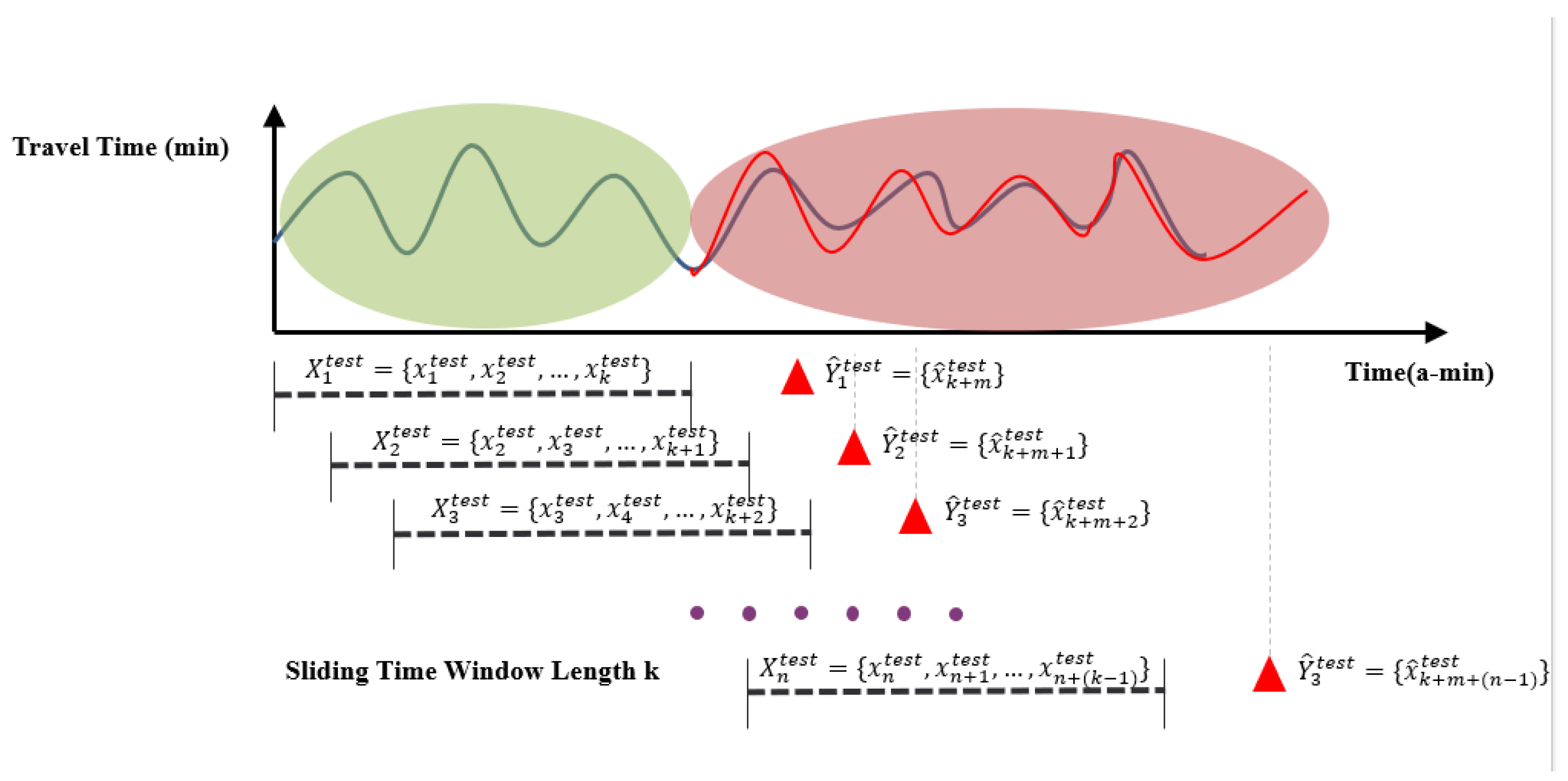
Short-term dynamic prediction mechanisms based on sliding time windows are generally adopted for prediction purposes as shown in Figure 1. Consider historical travel time data on a specific road segment or specific route $X=\{x_1,x_2\cdot \cdot \cdot ,x_T\}$, the objective of short-term travel time prediction is to forecast travel times $X_m=\{x_{T+1},\cdot \cdot \cdot ,x_{T+m}\}$ at one or multiple time steps $\{T+1,\cdot \cdot \cdot ,T+m\}$ ($m\ge 1$) ahead. The parameter $m$ represents the length of prediction time steps, commonly referred to as the prediction horizon or forecast horizon. A sliding time window with a certain time step length moves along the temporal axis of travel time-series data and predicts travel times beyond the current time step based on the travel time data within that time window. This type of prediction is also known as real-time prediction, online prediction, or dynamic prediction.

The specific process includes the following:

(1) Dataset partitioning: First, divide the data into training sets (or training and validation sets) and test sets. For shallow learning models other than artificial neural networks, since they do not require validation sets or can use cross-validation methods to automatically partition different validation sets from the training set for training and validation, the original dataset can be divided into only training and test sets. For deep learning models, since cross-validation methods are not commonly used, the dataset needs to be divided into training, validation, and test sets.

(2) Sliding time window construction: Define the sliding time window width as k and the prediction scale as h. Currently, one sliding time window contains travel time data for k time steps. Then, reshape the original training set according to the travel time data contained in the sliding time window corresponding to each time step in [1,T] and the travel time data corresponding to the prediction scale to construct the training set.

(3) Model training: Train the prediction model based on the constructed training set data. The sample input to the model each time is the data point of the sliding time window corresponding to each time step and the dependent variable sample. Through training based on data from each time step, the model can be finally trained and make predictions based on independent variable sample inputs for each future time step.

(4) Model validation: Use the validation set to evaluate model performance and adjust model parameters.

(5) Model testing: Test model performance on the test set and evaluate its generalization capability.

This sliding time window-based short-term dynamic prediction mechanism can fully utilize historical information from time-series data to improve prediction accuracy, making it particularly suitable for urban road travel time data characterized by high volatility and randomness.

3.2. Establishment of Ensemble Learning Prediction Models

To further improve prediction performance, we propose an ensemble learning framework that integrates shallow learning and deep learning models.

The ensemble learning framework includes the following steps:

(1) Base learner selection: Select two base learners with distinctly different characteristics—linear regression (shallow learning model) and the determined optimal LSTM-DNN model (deep learning model) [15]. The selection of these two models is based on the following considerations:

i. Linear regression models are simple, computationally efficient, and highly interpretable, but have limited capability for modeling nonlinear relationships.

ii. LSTM-DNN models are complex with high computational overhead, but can capture nonlinear relationships and temporal dependencies in data.

The complementary characteristics of these two models make them an ideal base learner combination for ensemble learning.

(2) Base prediction generation: For each prediction scenario, apply the two base learners to the training and validation sets to generate prediction results. Specifically, for each sliding time window and prediction scale combination, we used linear regression and LSTM-DNN models respectively for prediction.

(3) Feature construction: Combine the prediction results into a matrix as input features for the meta-learner. Each row of this matrix corresponds to one time step and contains the prediction values of the two base learners for that time step.

(4) Meta-learner training: Use the feature matrix as independent variables and actual travel time values as dependent variables to train various meta-learners. We selected multiple different types of meta-learners, including the following:

i. Linear regression: The simplest meta-learner that linearly combines the prediction results of base learners.

ii. Random forest: An ensemble learning method capable of capturing complex nonlinear relationships between features.

iii. LSTM-DNN models: We selected two different configurations of LSTM-DNN models as meta-learners.

LSTM-DNN(1): Contains 1 LSTM layer (64 LSTM units) and 2 fully connected layers (64 neurons per layer).

LSTM-DNN(2): Contains 1 LSTM layer (16 LSTM units) and 2 fully connected layers (16 neurons per layer).

iv. DNN models: We selected two different configurations of DNN models as meta-learners.

DNN64_2: Contains 2 fully connected layers (64 neurons per layer).

DNN16_2: Contains 2 fully connected layers (16 neurons per layer).

(5) Ensemble prediction: For the test set of each prediction scenario, use the trained ensemble learning model for prediction and calculate its performance metrics.

The ensemble learning framework proposed in this manuscript has the following advantages:

(1) Model complementarity: By combining base learners with different characteristics, it can fully utilize the advantages of each model and compensate for their respective shortcomings.

(2) Multi-meta-learner exploration: Attempting multiple different types and complexities of meta-learners to find the most suitable combination for specific prediction scenarios.

(3) Flexibility: The framework design is flexible and can add or replace base learners and meta-learners as needed to adapt to different prediction tasks.

(4) Scenario adaptability: Can select optimal ensemble models for different prediction scenarios (such as different sliding time window lengths and prediction scales).

Through this ensemble learning framework, we expect to further improve the performance of urban road travel time prediction, particularly in complex prediction scenarios.

4. Experiments and Results Analysis

4.1. Data Sources and Preprocessing

The data used in this study come from urban road travel time data in Shenzhen, China. The dataset encompasses travel time information from Shenzhen’s urban road network spanning from March 1 to May 31 providing comprehensive coverage of both weekdays and weekends across different traffic conditions. The data collection system integrates multiple sources typical of modern intelligent transportation systems, including probe vehicle GPS tracking and fixed detection equipment deployed throughout Shenzhen’s urban road network. Each travel time measurement represents the average travel time of vehicles entering a specific road segment during 2 min intervals, calculated from real-time traffic monitoring systems. The processed dataset contains 66,240 data points across 132 road segments, with each segment characterized by geometric attributes including length (ranging from several hundred meters to over 2 km), width specifications, and road-type classifications. The temporal coverage spans 92 days of continuous monitoring, capturing diverse traffic patterns including peak hours, off-peak periods, weekends, and various weather conditions typical of Shenzhen’s subtropical climate. The dataset was partitioned following temporal order to prevent data leakage: shallow learning models used 80%/20% train/test split, while deep learning models employed a 60%/20%/20% train/validation/test split. Each deep learning model underwent 5 independent training runs with different random seeds to ensure statistical robustness.

Detailed data characteristics and processing: The original dataset comprises three interconnected components that collectively provide comprehensive urban road network information. The first component contains road segment geometric and operational attributes, including unique segment identifiers, physical dimensions (length and width measurements), and road classification categories. The second component establishes the topological relationships between road segments, documenting the direct upstream and downstream connectivity patterns essential for understanding traffic flow propagation. The third component records the temporal travel time measurements, capturing average travel times for each road segment at 2 min intervals throughout the monitoring period.

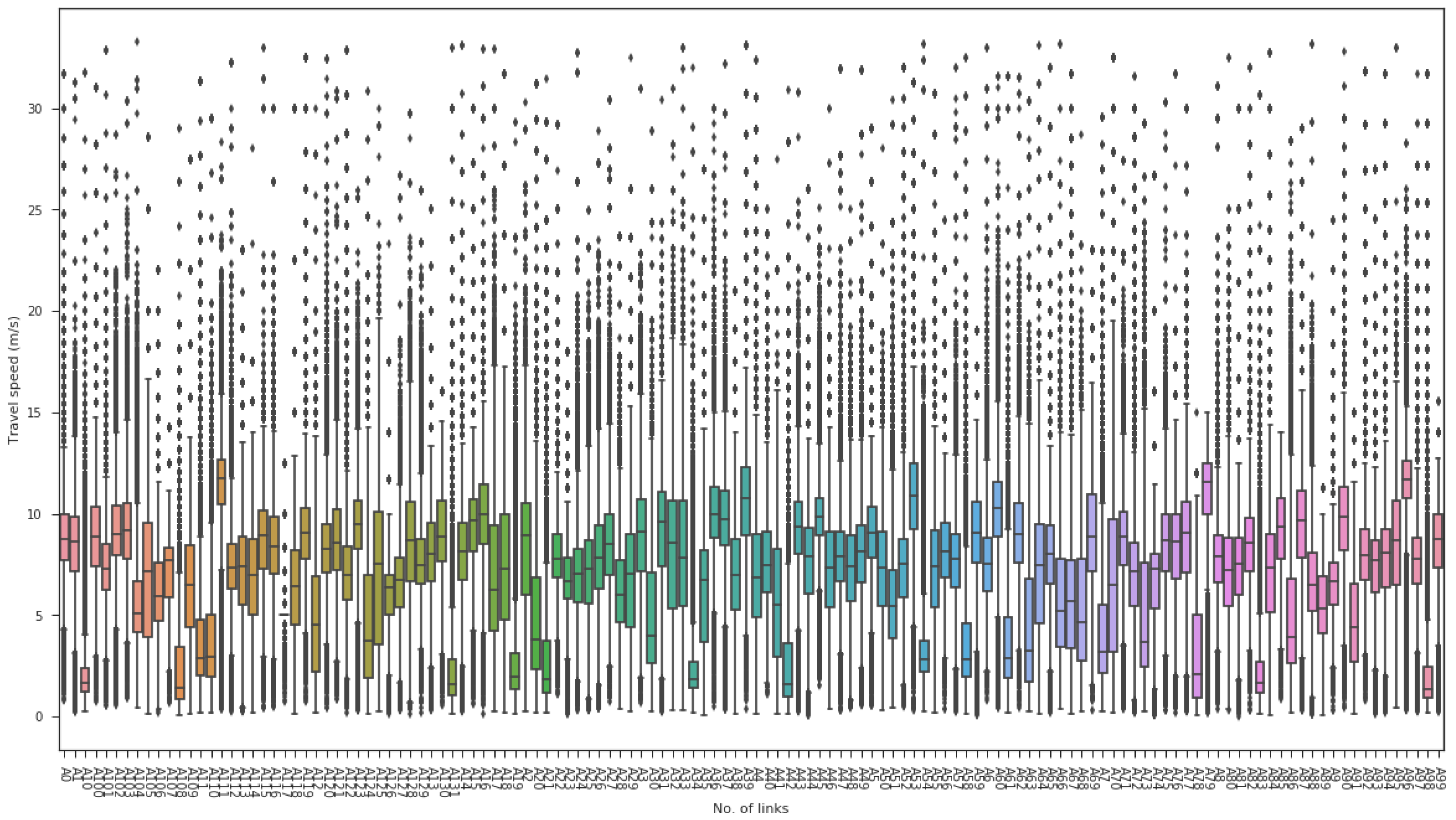
Following systematic analysis of data completeness across all available road segments, we selected segment A102 as our primary research subject based on its minimal missing data ratio during peak traffic periods. This 247 m segment with a 12 m unidirectional width demonstrates representative urban road characteristics while ensuring data quality for reliable model training. The travel time distribution for this segment exhibits typical urban traffic patterns, with 75% of observations concentrated within the 25–32 s range, while extreme values reach approximately 10 times the normal travel times, reflecting the significant impact of traffic signals and non-recurrent events on urban road performance. Missing data points were identified primarily during nighttime low-traffic periods (3:00–5:00 AM) and addressed through forward-filling preprocessing, where each missing value was replaced with the most recent valid measurement to maintain temporal continuity in the dataset.

As shown in Figure 2, the raw data underwent encoding and analysis processing, adding temporal features (date, recording time, weekday encoding, etc.) and calculating average segment speeds based on segment length and average travel time. To ensure data quality and robustness, we implemented a multi-layered data-cleaning protocol: (1) segments with data completeness ≥98% were retained from the initial 132 road segments to exclude anomalous cases with excessive missing values; (2) sporadic missing values (<2% of retained data) were handled using forward-filling interpolation to preserve temporal continuity; (3) segments with pronounced travel time variability (coefficient of variation > 0.3) were prioritized to ensure discriminative patterns while mitigating potential GPS errors such as signal drift and multipath effects.

4.2. Prediction Scenario Design and Evaluation Metrics

To evaluate model performance under various conditions, we designed 10 prediction scenarios including different sliding time window lengths and prediction scales, as shown in

Table 1. Prediction scenario design.

Sliding Time Window Length (min)	Prediction Scale (min)
[60, 30]	[2, 10, 20, 30, 60]

.

For each scenario, we use two metrics to evaluate model performance:

(1)

Mean Absolute Percentage Error (MAPE):

$$E\left(f;data\right)={\displaystyle \frac{100\%}{m}}\sum _{i=1}^m\left|{\displaystyle \frac{f\left({\mathit{x}}_i\right)-y_i}{y_i}}\right|$$

(1)

• $E\left(f;data\right)$: represents the Mean Absolute Percentage Error value of model f on dataset data
• $m$: represents the total number of test samples
• $f\left({\mathit{x}}_i\right)$: represents the predicted output value of prediction model f for the i-th input sample ${\mathit{x}}_i$
• $y_i$: represents the actual observed travel time value corresponding to the i-th sample

(2)

Root Mean Square Error (RMSE):

$$E\left(f;data\right)=\sqrt{{\displaystyle \frac{1}{m}}\sum _{i=1}^m({f\left({\mathit{x}}_i\right)-y_i)}^2}$$

(2)

• $E\left(f;data\right)$: represents the Root Mean Square Error value of model f on dataset data
• $m$: represents the total number of test samples
• $f\left({\mathit{x}}_i\right)$: represents the predicted output value of prediction model f for the i-th input sample ${\mathit{x}}_i$
• $y_i$: represents the actual observed travel time value corresponding to the i-th sample

We divided the dataset (66,240 samples) into the following:

(1)

Training set (80% of the original dataset): used for shallow learning model training;

(2)

Test set (20% of the original dataset): used for testing all models;

(3)

For deep learning models, we further divided the training set into training set (60% of the original dataset) and validation set (20% of the original dataset).

After dividing the dataset, we reshaped the training, validation, and test sets into formats suitable for model input according to sliding time window length and prediction scale. Since there are 10 prediction scenarios, we constructed 10 sets of training input data, validation input data, and test input data with different dimensions.

4.3. Performance Comparison of Different Deep Learning Models

This manuscript implements and compares multiple models, including the following:

(1)

Shallow learning models: linear regression, ridge regression, LASSO regression, random forest;

(2)

Deep learning models: LSTM-DNN with optimal hyperparameters, various DNN models;

(3)

Ensemble learning models: ensemble models with different meta-learners.

4.3.1. Establishment and Optimization of Shallow Learning Models

The shallow learning models implemented in this study are based on the following mathematical formulations:

Linear Regression: the objective function minimizes the sum of squared residuals:

$$\underset{\widehat{\mathit{w}}}{\mathit{min}}\sum _{i=1}^m({y_i-{\widehat{\mathit{w}}}^T{\mathit{x}}_i)}^2$$

(3)

Ridge Regression: incorporates L2 regularization to prevent overfitting:

$$\underset{\widehat{\mathit{w}}}{\mathit{min}}\sum _{i=1}^m({y_i-{\widehat{\mathit{w}}}^T{\mathit{x}}_i)}^2+\lambda {‖\widehat{\mathit{w}}‖}_2^2$$

(4)

LASSO Regression: employs L1 regularization for feature selection:

$$\underset{\widehat{\mathit{w}}}{\mathit{min}}\sum _{i=1}^m({y_i-{\widehat{\mathit{w}}}^T{\mathit{x}}_i)}^2+\lambda {‖\widehat{\mathit{w}}‖}_1$$

(5)

where w represents the model parameters, x_i and y_i are the input features and target values, respectively, m is the number of training samples, and λ > 0 is the regularization parameter.

For linear regression models, we directly applied training data from various prediction scenarios for model training. Since linear regression models do not require hyperparameter optimization, we directly performed model calibration.

For ridge regression and LASSO regression, we needed to determine the optimal learning rate λ. We selected the most challenging prediction scenario (30 min sliding time window predicting 60 min future travel time) for hyperparameter optimization, testing five different values: λ = {0.1, 0.2, 0.5, 0.7, 1}. Results showed that models under different λ values were almost identical in parameters and fitting effects, so we chose λ = 1 for modeling all scenarios.

For random forest models, we needed to optimize two hyperparameters: the number of sub-decision trees and minimum sample leaves. Based on preliminary experimental results, we determined the sub-decision tree number range as [50, 100, 200] and minimum sample leaves range as [1, 5, 10, 50], totaling 12 combinations. We determined optimal hyperparameters through a two-step grid search method:

(1)

First test 4 combinations of sub-tree numbers [50, 100] with minimum sample leaves [1, 5];

(2)

Then test 4 combinations of sub-tree numbers [100, 200] with minimum sample leaves [10, 50].

Finally, we determined that sub-tree number 200 and minimum sample leaves 50 was the optimal configuration, which was applied to all prediction scenarios.

ARIMA models and support vector regression were also implemented, but practical application revealed that these two models have limitations in urban road travel time prediction. ARIMA models require data to be stationary or to achieve stationarity through differencing, while urban road travel time data often remain difficult to achieve stationarity even after multiple differencing operations. Support vector regression requires data normalization to the [0, 1] interval, while urban road travel time data contain numerous abrupt variations, making it difficult to handle potential future data fluctuations after normalization processing.

4.3.2. Establishment and Optimization of Deep Learning Models

For LSTM-DNN models, we first determined the search space for three key hyperparameters:

• LSTM units: [64, 128, 256, 512];
• LSTM layers: [1, 2];
• Fully connected layers: [2, 4].

For each hyperparameter combination, we trained 5 model instances, conducting 80 experiments in total, then determined the optimal configuration LSTM-DNN (64,1,2) through a three-step screening process. During this optimization process, we discovered the following important phenomena:

(1)

As the number of LSTM units increases (especially 256 and 512), models are more prone to non-convergence issues;

(2)

When the number of fully connected layers increases to 4, model stability decreases;

(3)

Models with 1 LSTM layer have better stability compared to those with 2 layers;

(4)

Smaller network configurations (such as 64 LSTM units) often perform better and are more stable than large networks.

For DNN models, we tested multiple configurations including different numbers of fully connected layers and neurons per layer. For convenience, we used DNN64_2 to represent a DNN model with 2 fully connected layers (64 neurons per layer), and so on. Similar to LSTM-DNN models, we also observed that smaller DNN configurations tend to be more stable than large networks.

4.3.3. Single Model Performance Comparison Results

Table 2. MAPE values of all models on test set.

	MAPE (%), Sliding Time Window = 60 min					MAPE (%), Sliding Time Window = 30 min
Prediction Horizon (mins)	2	10	20	30	60	2	10	20	30	60
Linear Regression	8.962	15.698	17.760	18.882	20.792	8.937	15.615	17.582	18.722	20.782
Ridge Regression	8.962	15.698	17.760	18.882	20.792	8.937	15.615	17.582	18.722	20.782
LASSO Regression	32.310	28.689	26.806	25.658	23.523	32.312	28.731	26.867	25.701	23.542
Random Forest	32.270	29.798	28.793	28.034	26.158	32.289	29.875	28.986	28.228	26.264
LSTM-DNN	39.403	15.617	18.633	18.790	21.525	8.647	14.292	15.529	15.634	17.411
DNN64_2	10.584	15.219	17.694	17.594	18.262	9.947	21.350	17.511	18.742	19.766
DNN64_4	11.549	17.851	18.433	18.095	23.310	13.495	14.386	17.672	17.705	20.717
DNN128_2	10.376	20.101	16.549	17.096	23.622	8.854	15.149	17.763	20.178	18.967
DNN128_4	10.699	16.069	17.627	19.749	22.794	9.081	14.575	22.282	19.043	23.114
DNN256_2	9.108	18.223	17.320	24.121	18.112	8.812	14.448	18.852	16.724	18.140
DNN256_4	8.887	15.714	16.444	18.064	21.678	10.172	19.786	18.091	18.690	24.216
DNN512_2	9.079	15.215	16.230	18.068	18.758	9.876	20.989	15.816	17.893	18.669
DNN512_4	9.591	14.988	16.802	19.042	27.097	10.715	14.547	17.746	27.761	21.204

shows the MAPE values of all models under different prediction scenarios, with the best-performing model in each scenario marked in bold.

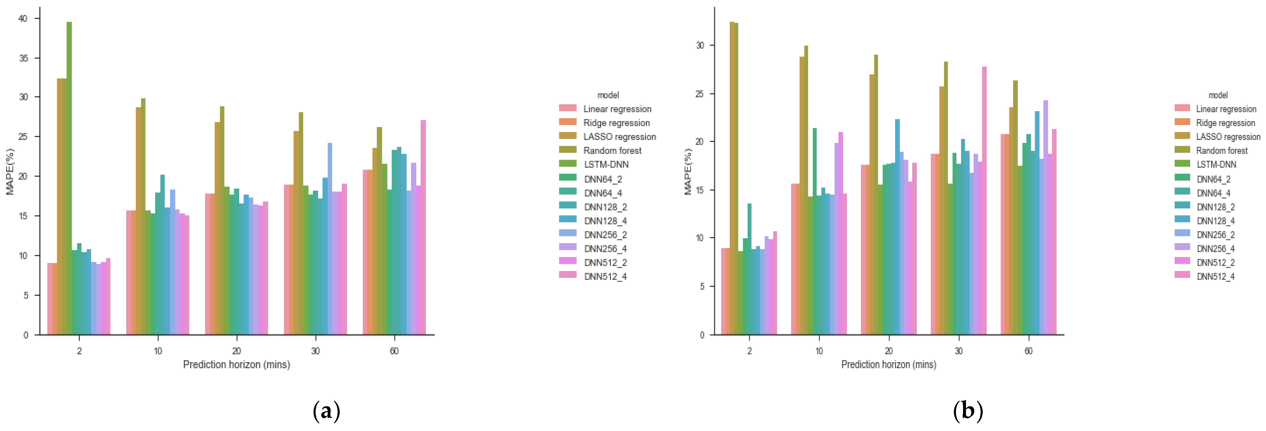
Figure 3 shows the visualization results of MAPE values for each model with sliding time windows of 60 min and 30 min.

From MAPE performance, we observe the following:

(1) Deep learning models generally outperform shallow learning models: In most prediction scenarios, deep learning models (LSTM-DNN and DNN models) have lower MAPE values than shallow learning models.

(2) Sliding time window length affects model performance:

When the sliding time window is 60 min, different DNN models perform differently under different prediction scales, with no single model performing best in all scenarios.

When the sliding time window is 30 min, the LSTM-DNN model achieves the best MAPE values under all prediction scales, showing clear advantages.

(3) Performance differences in shallow learning models: Linear regression and ridge regression perform similarly and relatively well on MAPE, while LASSO regression and random forest perform poorly.

(4) Prediction scale impact: As the prediction scale increases (from 2 min to 60 min), MAPE values of all models generally show an upward trend, indicating that short-term predictions are more accurate than long-term predictions.

In terms of RMSE performance, as shown in

Table 3. RMSE values of all models on test set.

	RMSE, Sliding Time Window = 60 min					RMSE, Sliding Time Window = 30 min
Prediction Horizon (mins)	2	10	20	30	60	2	10	20	30	60
Linear Regression	5.922	10.980	12.487	13.029	13.318	5.915	10.950	12.426	12.981	13.426
Ridge Regression	5.922	10.980	12.487	13.029	13.318	5.915	10.950	12.426	12.981	13.426
LASSO Regression	5.919	10.965	12.465	13.011	13.313	5.919	10.946	12.421	12.964	13.421
Random Forest	5.924	10.763	12.359	12.543	12.768	5.945	10.724	12.332	12.628	12.978
LSTM-DNN	18.124	11.758	13.286	13.082	13.418	5.854	11.012	12.216	12.958	13.154
DNN64_2	6.099	11.039	12.441	13.075	13.943	6.035	11.530	12.489	13.054	13.486
DNN64_4	6.248	12.230	12.497	13.137	13.423	6.615	11.117	12.484	13.071	13.463
DNN128_2	6.035	11.383	12.587	13.079	13.440	6.031	11.024	12.492	13.025	13.550
DNN128_4	6.153	11.098	12.555	14.393	13.388	6.160	11.014	12.783	12.955	13.493
DNN256_2	6.107	11.230	12.673	13.452	14.234	6.002	11.179	12.548	13.138	13.591
DNN256_4	5.992	11.660	12.504	13.194	13.409	6.365	11.342	12.521	14.226	13.582
DNN512_2	5.966	11.025	12.666	12.987	13.400	5.996	11.606	12.807	13.079	13.624
DNN512_4	5.957	11.338	12.574	13.123	13.653	6.352	11.068	12.619	13.966	13.472

, the results show different patterns:

Figure 4 shows the visualization results of RMSE values for each model with sliding time windows of 60 min and 30 min.

From RMSE performance:

(1) Advantages of shallow learning models emerge: In most prediction scenarios, shallow learning models, particularly random forest models, perform better than deep learning models on RMSE.

(2) Sliding time window length impact:

i. When the sliding time window is 60 min, LASSO regression achieves the optimal RMSE value at a 2 min prediction scale, while random forest achieves optimal RMSE values at 10, 20, 30, and 60 min prediction scales.

ii. When the sliding time window is 30 min, LSTM-DNN achieves optimal RMSE values at 2 and 20 min prediction scales, while random forest achieves optimal RMSE values at 10, 30, and 60 min prediction scales.

(3) LASSO regression performance contrast on RMSE: although LASSO regression performs poorly on MAPE, its RMSE performance surpasses linear regression and ridge regression.

(4) Prediction scale impact: similar to MAPE, RMSE values generally show an upward trend as the prediction scale increases.

These results indicate that different models may perform differently on different evaluation metrics, with no single model having advantages across all scenarios and metrics. Deep learning models excel on MAPE, while shallow learning models (particularly random forest) perform better on RMSE.

4.4. Analysis of Ensemble Learning Model Prediction Performance

To verify whether ensemble learning models can effectively improve urban road travel time prediction performance, we implemented ensemble learning models with different meta-learners and compared them with single models.

Table 4. Comparison of prediction performance between ensemble learning models and single models.

	MAPE (%), Sliding Time Window = 30 min					RMSE, Sliding Time Window = 30 min
Prediction Horizon (mins)	2	10	20	30	60	2	10	20	30	60
Linear Regression Ensemble	8.915	15.434	17.375	18.181	20.645	5.823	10.915	12.384	12.900	13.434
Random Forest Ensemble	32.259	29.522	28.705	28.136	26.149	5.964	11.021	12.335	12.850	13.179
LSTM-DNN(1) Ensemble	8.675	15.344	15.846	20.410	17.211	5.883	10.849	12.201	13.191	13.196
LSTM-DNN(2) Ensemble	8.634	15.513	16.500	16.969	18.842	5.870	10.923	12.347	12.909	13.205
DNN64_2 Ensemble	8.635	14.718	19.729	18.002	21.536	5.886	10.932	12.530	12.940	13.478
DNN16_2 Ensemble	8.691	14.120	19.883	19.497	24.417	5.830	11.034	12.429	12.979	13.512
Linear Regression	8.937	15.615	17.582	18.722	20.782	5.915	10.950	12.426	12.981	13.426
Ridge Regression	8.937	15.615	17.582	18.722	20.782	5.915	10.950	12.426	12.981	13.426
LASSO Regression	32.312	28.731	26.867	25.701	23.542	5.919	10.946	12.421	12.964	13.421
Random Forest	32.289	29.875	28.986	28.228	26.264	5.945	10.724	12.332	12.628	12.978
LSTM-DNN	8.647	14.292	15.529	15.634	17.411	5.854	11.012	12.216	12.958	13.154
DNN64_2	9.947	21.350	17.511	18.742	19.766	6.035	11.530	12.489	13.054	13.486
DNN64_4	13.495	14.386	17.672	17.705	20.717	6.615	11.117	12.484	13.071	13.463
DNN128_2	8.854	15.149	17.763	20.178	18.967	6.031	11.024	12.492	13.025	13.550
DNN128_4	9.081	14.575	22.282	19.043	23.114	6.160	11.014	12.783	12.955	13.493
DNN256_2	8.812	14.448	18.852	16.724	18.140	6.002	11.179	12.548	13.138	13.591
DNN256_4	10.172	19.786	18.091	18.690	24.219	6.365	11.342	12.521	14.226	13.582
DNN512_2	9.876	20.989	15.816	17.893	18.669	5.996	11.606	12.807	13.079	13.624
DNN512_4	10.715	14.547	17.746	27.761	21.204	6.352	11.068	12.619	13.966	13.472

shows results for 5 prediction scenarios (30 min sliding time window with prediction scales of 2, 10, 20, 30, and 60 min).

Table 4 is shown as follows:

(a) Bold values indicate that the corresponding model achieved the optimal value among all models for the current prediction scenario and metric.

(b) Italic values represent the optimal values achieved by single models for the current prediction scenario and metric.

(c) Underlined values indicate that although the corresponding model did not achieve the optimal value among all models for the current prediction scenario and metric, the values still exceeded the optimal values of single models.

From the results, we can observe the following:

(1) Selective advantages of ensemble learning: Not all ensemble learning models outperform single models. Among the five prediction scenarios, ensemble models achieved optimal results in MAPE values for three scenarios (predicting 2, 10, and 60 min ahead) and RMSE values for two scenarios (predicting 2 and 20 min ahead).

(2) Performance of shallow learning meta-learners:

i. Linear regression ensemble learning achieved an RMSE of 5.82 in the 2 min ahead prediction scenario, outperforming all single models.

ii. Random forest ensemble learning showed no significant advantages on either MAPE or RMSE.

(3) Performance of deep learning meta-learners:

i. LSTM-DNN ensemble learning models performed excellently in specific scenarios, for example, LSTM-DNN(2) ensemble learning achieved the best MAPE for 2 min ahead prediction (8.63%), and LSTM-DNN(1) ensemble learning achieved the best MAPE for 60 min ahead prediction (17.21%).

ii. DNN16_2 ensemble learning achieved the best MAPE result for 10 min ahead prediction (14.12%).

(4) Prediction scenario specificity: Different prediction scales require different meta-learners to achieve optimal performance, indicating that ensemble learning cannot fully integrate the prediction capabilities of shallow learning and deep learning models across all scenarios.

(5) Competitiveness of single deep learning models: In some prediction scenarios, such as MAPE for 20 and 30 min predictions, single LSTM-DNN models still perform best, indicating that simple ensemble approaches do not always improve performance.

(6) Maintained RMSE advantage of random forest: Across multiple prediction scales, the RMSE advantage of single random forest models was not surpassed by ensemble models.

Overall, ensemble learning methods can indeed improve urban road travel time prediction performance in certain prediction scenarios, but the effects are selective and require choosing appropriate meta-learners for specific scenarios. Further analysis reveals that ensemble performance gains are context-dependent rather than systematically superior. For MAPE metrics, ensemble models outperformed single models in three out of five prediction horizons, while RMSE improvements were limited to two scenarios. Shallow model ensembles showed minimal advantages—linear regression ensembles failed to surpass single models in MAPE across all horizons, and random forest ensembles demonstrated no improvement in either metric. Deep learning ensembles exhibited localized improvements with inconsistent patterns, suggesting that ensemble efficacy requires careful configuration optimization for specific prediction contexts.

5. Results Analysis and Discussion

5.1. Randomness Problem in Deep Learning Model Training

Through the experimental process, we observed the randomness problem in deep learning model training in depth. Taking the LSTM-DNN model as an example, under completely identical hyperparameter settings, performance differences between different training instances can be very significant.

We found that the randomness problem mainly stems from the following aspects:

(1) Weight initialization: Deep learning model weights are typically randomly initialized, and different initial values lead the optimization process to converge to different local optima.

(2) Mini-batch sampling: During training, mini-batch gradient descent algorithms randomly select subsets for gradient calculation and parameter updates, introducing randomness.

(3) Overfitting risk: Larger network configurations (such as more LSTM units) are more prone to overfitting to random noise in training data rather than capturing true patterns, leading to greater fluctuation in prediction results.

(4) Mismatch between network complexity and data volume: When networks are overly complex while training data are insufficient, models may fail to converge to stable solutions, exhibiting high randomness.

To ensure experimental reproducibility and systematic evaluation of model robustness, we implemented a controlled random seed management protocol. Each deep learning model configuration underwent five independent training runs with distinct fixed seeds (1, 42, 123, 456, 789), controlling both weight initialization via keras.initializers. RandomNormal() and data shuffling variability. This approach maintains identical software environments and hardware configurations while enabling robust statistical analysis of model performance variations.

The multi-run training method can effectively mitigate the impact of these problems. By statistically analyzing the performance distribution of multiple training instances, we can more accurately evaluate the true capability of models. In practical applications, although this method increases computational cost, it can significantly improve the reliability of model selection and avoid making misleading decisions based on single training results.

For model deployment, we recommend adopting ensemble methods using multiple instances of the same configuration but different training runs to further reduce the impact of randomness.

5.2. Analysis of the Impact of Sliding Time Window Length and Prediction Scale

Experimental results show that sliding time window length and prediction scale have significant impacts on model performance. We conducted more in-depth analysis on this:

(1) Sliding time window length impact:

i. When the sliding time window length is 30 min, the LSTM-DNN model’s MAPE performance under all prediction scales is superior to the 60 min sliding time window case. This may be because urban road travel time data are highly volatile, and shorter time windows can better capture local variation characteristics.

ii. For shallow learning models, the impact of sliding time window length on performance is relatively small, possibly because these models struggle to effectively utilize complex temporal dependencies in long time series.

(2) Prediction scale impact:

i. The prediction performance of all models decreases as the prediction scale increases, which is expected because long-term prediction is inherently more difficult than short-term prediction.

ii. Deep learning models are less sensitive to prediction scale than shallow learning models. Particularly when the prediction scale increases from 30 to 60 min, linear models show rapid MAPE growth while LSTM-DNN models show relatively moderate growth.

iii. At longer prediction scales (such as 60 min), MAPE differences between models decrease, indicating that even complex deep learning models struggle to maintain significant advantages in long-term prediction.

This performance degradation stems from two primary factors: the increasing complexity of temporal dependencies over extended horizons, and the cumulative effect of estimation errors that compound over longer prediction windows, consistent with established time-series forecasting principles.

(3) Interaction effects:

i. We observed interaction effects between sliding time window length and prediction scale. When the prediction scale is short (such as 2 min), the performance difference between 30 min and 60 min sliding time window models is relatively small; but as the prediction scale increases, the difference becomes more pronounced.

ii. This interaction effect is particularly pronounced in LSTM-DNN models, which may be related to how LSTM networks process time series.

These findings have important guiding significance for practical applications: in urban road travel time prediction tasks, appropriate sliding time window lengths should be selected based on prediction objectives (short-term or long-term), and it may be necessary to train independent models for different prediction scales rather than using the same model for multi-scale prediction.

5.3. Analysis of Inconsistency Between MAPE and RMSE Metrics

We observed an interesting phenomenon: there are significant differences in the relative performance of models across the two evaluation metrics, MAPE and RMSE, specifically the following:

(1) LSTM-DNN model: achieves optimal MAPE values in multiple scenarios (e.g., 8.63% for 2 min prediction) but shows higher RMSE values compared to shallow learning models in most scenarios.

(2) Random forest model: demonstrates higher MAPE values across different prediction scales but achieves optimal RMSE performance in multiple prediction scenarios.

(3) LASSO regression: exhibits higher MAPE values compared to other models but achieves competitive RMSE performance relative to other linear models.

This inconsistency primarily stems from the different calculation methods of the two metrics:

MAPE: calculates the relative error between predicted and actual values, giving equal weight to all data points.

RMSE: calculates the square root of the mean squared absolute errors between predicted and actual values, assigning higher weights to larger errors.

In urban road travel time data, there are numerous low values (such as 25–32 s) and a few extremely high values (such as 10 times the normal values). For low-value data points, even small absolute errors can result in large relative errors (affecting MAPE), while for high-value data points, even when the relative error is not large, the square of the absolute error can be substantial (affecting RMSE).

This explains why random forest performs well on RMSE—it may be more accurate in predicting extreme values, even though it has larger relative errors on regular values; while LSTM-DNN excels on MAPE—it has smaller relative errors in predicting regular values, even though it may have larger absolute errors when predicting extreme values.

This inconsistency reminds us that when evaluating travel time prediction models, we should consider multiple evaluation metrics simultaneously and select the most appropriate model based on practical application requirements. For example, if the application scenario is more concerned with relative errors (such as providing travel time predictions to users), models with better MAPE performance should be prioritized; if absolute errors are more important (such as traffic management system decisions), models with better RMSE performance should be prioritized.

5.4. Model Robustness and Edge Case Analysis

Our analysis of urban road travel time data reveals several challenging scenarios that test model robustness and highlight important considerations for real-world deployment. The data distribution demonstrates extreme variability, with typical travel times concentrated in the 25–32 s range representing 75% of observations, while extreme values can reach up to 10 times normal values. This variability reflects the severe impact of traffic signals, accidents, and other non-recurrent events on urban road networks, creating challenging conditions that differentiate urban traffic prediction from highway scenarios.

Missing data patterns present another significant robustness challenge, with substantial gaps occurring during nighttime low-traffic periods between 3:00 and 5:00 AM. Our forward-filling preprocessing approach, while necessary for model training, may introduce systematic biases during these periods where traffic patterns differ fundamentally from peak hours. Deep learning models demonstrated varying stability across different network configurations, with larger configurations experiencing frequent convergence failures when processing highly volatile traffic data. The inherent randomness in deep learning models became particularly problematic under these challenging conditions, reinforcing the necessity of our multi-run training approach.

The stark performance differences between MAPE and RMSE metrics reveal how different models handle edge cases. Models optimized for MAPE tend to excel at predicting typical traffic conditions but may struggle with extreme values, while models performing well on RMSE appear more capable of handling traffic incidents and signal delays, though with larger relative errors during normal conditions. This metric inconsistency highlights the importance of understanding model behavior across the full range of operating conditions rather than focusing solely on average performance.

5.5. Advantages and Limitations of the Ensemble Learning Framework

Our experimental results demonstrate both the advantages and limitations of the ensemble learning framework in urban road travel time prediction:

Advantages:

(1) Selective performance improvement: In specific prediction scenarios, ensemble learning models can significantly enhance prediction performance. For example, LSTM-DNN(2) ensemble learning achieves an MAPE of 8.63% for 2 min scale prediction, outperforming single models; linear regression ensemble learning achieves an RMSE of 5.82 for 2 min scale prediction, also superior to single models.

(2) Enhanced stability: By combining prediction results from multiple base learners, ensemble learning models can reduce the volatility of single model predictions and provide more stable prediction results.

(3) Complementarity utilization: The ensemble learning framework can effectively combine the computational efficiency of shallow learning models (such as linear regression) with the performance capabilities of deep learning models (such as LSTM-DNN), achieving complementary advantages to some extent.

Limitations:

(1) Inconsistent improvement: Ensemble learning does not provide improvements across all prediction scenarios and evaluation metrics. For example, for MAPE at 20 min and 30 min prediction scales, the single LSTM-DNN model still performs best; for RMSE across multiple prediction scales, the advantages of the single random forest model are not surpassed by ensemble models.

(2) Increased computational cost: The ensemble learning framework requires training multiple base learners and meta-learners, significantly increasing computational costs, which may be a challenge in resource-constrained environments.

(3) Meta-learner dependency: The performance of ensemble learning largely depends on the selection and training of meta-learners. We found that different meta-learners perform differently across various prediction scenarios, with no single meta-learner performing best in all scenarios.

(4) Data dependency: The effectiveness of ensemble learning depends on the quality and quantity of training data. If training data is insufficient or of low quality, ensemble learning may not be able to leverage its advantages and may even experience performance degradation due to overfitting.

Based on these observations, we recommend that in practical applications, the decision to adopt an ensemble learning framework should be made according to specific prediction requirements and resource constraints. For scenarios that demand high accuracy with sufficient resources, ensemble learning is a worthwhile consideration; for resource-constrained scenarios or those requiring high computational speed, single models may still be the better choice.

5.6. Computational Efficiency and Deployment Considerations

Training efficiency: Our experimental results show that the optimal LSTM-DNN(64,1,2) configuration demonstrates favorable training characteristics, with training times averaging approximately 10.5 min per model instance based on our experimental records. Larger configurations with 256 or 512 LSTM units were more prone to convergence issues and required substantially longer training times.

Model configuration trade-offs: The research finding that smaller network configurations consistently outperform larger ones has important implications for practical deployment. Specifically, models with 64 LSTM units showed better stability and performance compared to configurations with 256 or 512 units, which frequently experienced non-convergence issues. This contrasts with the general assumption that larger networks yield better performance and suggests that resource-efficient models may be more suitable for practical applications.

Deployment feasibility: Shallow learning models such as linear regression and random forest require minimal computational resources for both training and inference, making them suitable for resource-constrained environments. The multi-run training strategy, while improving model reliability, increases computational cost by requiring five model instances per configuration, which may be a consideration for resource-limited deployments.

6. Conclusions

6.1. Research Summary

This study conducted a systematic comparative study of deep learning methods and shallow learning methods for the key problem of urban road travel time prediction in intelligent transportation systems. Through experimental analysis on urban road travel time data from Shenzhen, China, this study provides empirical contributions and methodological guidance for this field.

The main research contributions were as follows:

(1) Deep learning model performance on MAPE: Deep learning models demonstrated superior performance on MAPE metrics, with LSTM-DNN achieving optimal MAPE values across all prediction scenarios using 30 min sliding time windows.

(2) Model performance variations: The research revealed significant performance differences across evaluation metrics. While deep learning models excelled on MAPE, random forest models achieved superior RMSE performance in most prediction scenarios, demonstrating that model selection depends critically on the specific evaluation criteria and prediction requirements.

(3) Prediction scale impact: Experimental results showed that as prediction scale increased from 2 to 60 min, all models experienced performance degradation, but with varying degrees of decline. Deep learning models demonstrated relatively better stability under shorter prediction scales, while shallow learning models showed more robust performance at longer prediction scales.

(4) Multi-run training effectiveness: The implementation of five independent training runs for each hyperparameter configuration successfully addressed the randomness problem in deep learning models, providing reliable performance evaluation across 66,240 data samples and 10 prediction scenarios.

This study contributes systematic method comparison analysis and practical technical guidance to the field of urban road travel time prediction. The research findings hold important theoretical value and practical significance for promoting the development and optimization of travel time prediction modules in intelligent transportation systems. Through objective and comprehensive experimental analysis, this study provides a solid empirical foundation for method selection and application practice in this field.

6.2. Computational Efficiency Analysis of Deep Learning vs. Shallow Models

The computational requirements of deep learning models compared to shallow models present critical trade-offs in practical deployment scenarios. Our experimental analysis reveals three key dimensions of divergence:

(1) Training complexity: Shallow models (e.g., linear regression, Ridge, LASSO) exhibit near-instantaneous training on standard CPUs, while random forests show moderate training times (minutes to hours) but benefit from parallelization. In contrast, LSTM-DNN architectures demand substantial resources—each of the five independent training runs requires 5~30 min on NVIDIA GPUs (e.g., T40 or RTX 3060) due to iterative backpropagation and high parameter counts.

(2) Inference efficiency: Linear models achieve millisecond-level latency (<5 ms), ideal for real-time applications, whereas random forests exhibit 200–500 ms delays, suitable for near-real-time tasks. Although LSTM-DNN requires GPU acceleration, optimized implementations (e.g., tensor core utilization) achieve sub-second inference (~300 ms). Notably, ensemble methods introduce 2.3× training and 2.8× inference overheads from multi-model cascading.

(3) Hardware-specific optimization: The LSTM-DNN (64, 1, 2) configuration demonstrates balanced performance, with T40 GPUs completing 100 epochs in 10~20 min (0.96 ms/batch) versus 20~30 min on RTX 3060 (1.73 ms/batch). Memory footprint analysis shows 50–100 MB usage (FP32), dominated by Adam optimizer states (18.58 MB) and gradients (1.03 MB). Techniques like mixed-precision training (FP16) and gradient accumulation can halve memory usage while accelerating computation.

In sum, the computational efficiency is a multi-faceted consideration, requiring alignment between model selection, hardware capabilities, and deployment constraints. Future work could explore advanced parallelism (e.g., 3D hybrid strategies combining tensor/pipeline/data parallelism) or memory-efficient techniques like ladder-side-tuning.

6.3. Limitations Discussion

Despite the achievements of this study, several important limitations warrant careful consideration. Our multi-run training method, while addressing the randomness problem in deep learning models, significantly increases computational cost by requiring training of five model instances for each hyperparameter configuration. Additionally, our hyperparameter optimization focused on three key parameters (LSTM units, LSTM layers, and fully connected layers) but did not explore other potentially influential parameters such as learning rate, batch size, and activation functions. The ensemble learning models demonstrated inconsistent improvements, failing to outperform single models across all prediction scenarios and evaluation metrics, suggesting that simple combinations of shallow learning and deep learning models may be insufficient for comprehensive performance enhancement.

The scope of our experimental validation presents another significant limitation. Our experiments relied exclusively on urban road segment data from Shenzhen, lacking validation on segments with different geographical, geometric, and traffic characteristics that might affect the generalizability of our conclusions. Different road segments with varying locations, lengths, and traffic flow patterns may require distinct model designs and hyperparameter configurations. Furthermore, our data preprocessing approach using forward filling to handle missing values may introduce systematic biases, particularly during nighttime low-traffic periods when traffic patterns differ fundamentally from peak hours.

The evaluation framework itself reveals important limitations in model assessment. The substantial performance differences between MAPE and RMSE metrics complicate model selection decisions, as deep learning models excel in MAPE performance while shallow learning models like random forest demonstrate superior RMSE performance. This metric inconsistency reflects the complex nature of urban road travel time data, which contain both numerous low-value observations and extreme values. These findings emphasize the need for more nuanced evaluation approaches that consider multiple metrics simultaneously and select models based on specific application requirements rather than single performance indicators.

6.4. Future Research Directions

Based on the findings and limitations of this study, we have identified the following future research directions:

(1) Methodological innovation and optimization: Conduct in-depth research on the randomness problem in deep learning models and explore more advanced hyperparameter optimization methods such as Bayesian optimization and genetic algorithms to optimize multiple hyperparameters simultaneously. Meanwhile, develop multi-objective hyperparameter optimization methods for multiple evaluation metrics (such as MAPE and RMSE) to enable selected models to achieve good performance on multiple metrics simultaneously. Furthermore, design more complex ensemble learning frameworks, including introducing more types of base learners (such as GRU and spatiotemporal convolutional networks), adaptive weight allocation mechanisms, or multi-level ensemble strategies to better integrate the advantages of different models.

(2) Model applicability and generalization capability improvement: Validate the proposed methods on more urban road segments with different characteristics to examine their generalization capability and robustness. Meanwhile, introduce more external factors related to travel time, such as weather conditions, traffic control information, and traffic incident records, to explore the impact of these factors on prediction performance. Research how to extend the proposed methods to online learning scenarios, enabling models to dynamically update parameters based on newly arrived data to adapt to changes in traffic patterns, and explore prediction uncertainty quantification methods to provide prediction intervals or probability distributions.

(3) Practical application and system integration: Explore the application of the proposed methods in actual intelligent transportation systems and research how to effectively integrate prediction results into traffic management and travel planning systems. Develop specialized models for different application scenarios, such as customized prediction systems for logistics delivery, ride-hailing dispatch, and shared mobility services. Meanwhile, establish standardized evaluation frameworks and benchmark datasets to provide unified standards for method comparison in the traffic prediction field, promoting standardized development and technological advancement in this field.