Two Decades of Groundwater Variability in Peru Using Satellite Gravimetry Data

Abstract

Groundwater is a critical yet understudied resource in Peru, where surface water has traditionally dominated national assessments. This study provides the first country-scale analysis of groundwater storage (GWS) variability in Peru from 2003 to 2023 using satellite gravimetry data from the Gravity Recovery and Climate Experiment (GRACE) and GRACE Follow-On (GRACE-FO) missions. We used the GRACE Data Assimilation-Data Mass Modeling (GRACE-DA-DM GLV3.0) dataset at 0.25° resolution to estimate annual GWS trends and evaluated the influence of El Niño–Southern Oscillation (ENSO) events and anthropogenic extraction, supported by in situ well data from six major aquifers. Results show a sustained GWS decline of 30–40% in coastal and Andean regions, especially in Lima, Ica, Arequipa, and Tacna, while the Amazon basin remained stable. Strong correlation (r = 0.95) between GRACE data and well records validate the findings. Annual precipitation analysis from 2003 to 2023, disaggregated by climatic zone, revealed nearly stable trends. Coastal El Niño events (2017 and 2023) triggered episodic recharge in the northern and central coastal regions, yet these were insufficient to reverse the sustained groundwater depletion. This research provides significant contributions to understanding the spatiotemporal dynamics of groundwater in Peru through the use of satellite gravimetry data with unprecedented spatial resolution. The findings reveal a sustained decline in GWS across key regions and underscore the urgent need to implement integrated water management strategies—such as artificial recharge, optimized irrigation, and satellite-based early warning systems—aimed at preserving the sustainability of the country’s groundwater resources.

1. Introduction

Groundwater is a critical resource for agriculture, industry, and domestic needs worldwide, supporting ecosystems and socioeconomic stability [1]. Its variability, driven by natural and human-induced factors, significantly affects water availability, making effective monitoring essential for sustainable water resource management. As pressures from population growth and climate change intensify, understanding GWS dynamics is increasingly vital to ensure long-term water security.

1.1. Satellite-Based Monitoring with GRACE

The Gravity Recovery and Climate Experiment (GRACE), launched in 2002, and its successor, GRACE Follow-On (GRACE-FO), developed by NASA and the German Aerospace Center (DLR), provide a powerful tool for monitoring GWS changes [2,3]. These satellites measure global gravitational field variations, enabling accurate estimates of water storage at regional and national scales. Over the past two decades, GRACE data have been used to assess groundwater fluctuations in regions such as the United States [4], Northern India [5], East Africa [6], and the Indus Basin in Pakistan [7], demonstrating the method’s reliability and scientific value [8,9,10,11]. This approach offers a scalable solution for studying groundwater in complex hydrogeological settings.

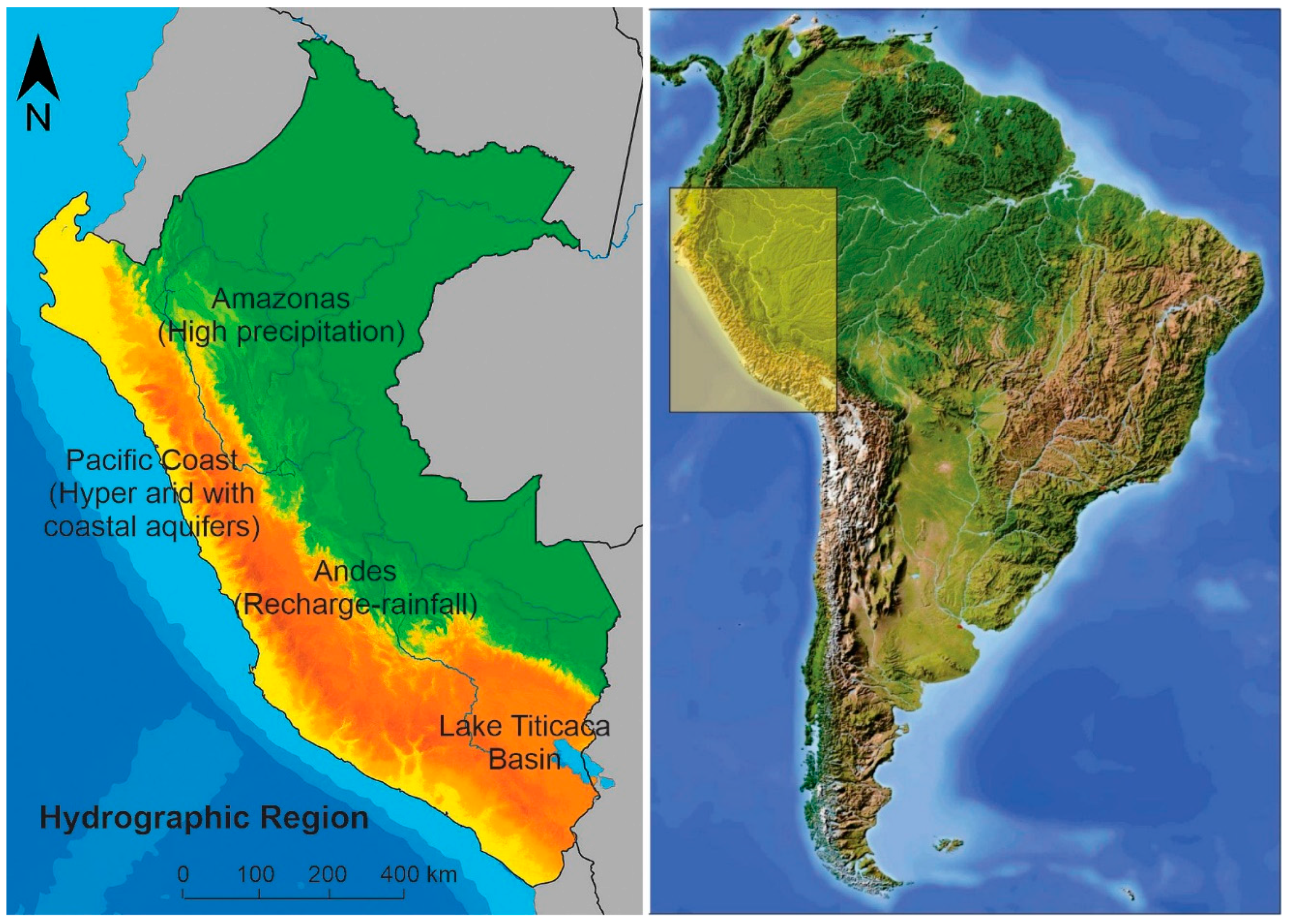
1.2. Hydrogeological Context of Peru

Peru’s diverse topography, encompassing coastal deserts, the Andes Mountains, and the Amazon Basin, creates a unique hydrogeological landscape heavily reliant on groundwater for agriculture, urban water supply, and ecosystems [12]. This heavy reliance on groundwater suggests that surface water storage in dams and reservoirs is either insufficient or not adequately distributed to meet agricultural and urban demand in various regions of the country. Coastal regions, such as Lima and Ica, face intense groundwater demand because of agricultural expansion, while Andean aquifers depend on snowmelt and precipitation, and the Amazon Basin benefits from high rainfall, but is vulnerable to deforestation [13]. This situation tends to decrease the GWS on the coast, keeps it conditioned in the Andes, and keeps it high or stable in the Amazon. These regional differences, combined with natural variability and anthropogenic pressures, underscore the need for comprehensive GWS assessments.

Peru faces growing challenges in groundwater management because of climate change, rapid urbanization, and agricultural intensification [14,15,16]. Precipitation variability, exacerbated by El Niño and La Niña events, disrupts recharge patterns and complicates water resource planning [17]. While multinational studies have included groundwater assessments in Peru [18,19,20,21,22], recent research has focused on specific issues, such as aquifer characterization [13,23], pollution and saline intrusion [19,24], groundwater-induced landslides [25,26], and sustainability in key regions like Ica and Piura [27,28]. Despite these efforts, most national-scale assessments have prioritized surface water, leaving critical gaps in understanding groundwater dynamics [29].

While regional studies have characterized specific aquifers (e.g., Ica, Piura) [27,28,29], there is a lack of comprehensive analyses that quantify GWS trends across Peru’s diverse coastal, Andean, and Amazonian regions over extended periods. Furthermore, few studies have integrated satellite gravimetry data with in situ measurements to validate GWS estimates or assessed the combined impacts of El Niño–Southern Oscillation (ENSO) events and anthropogenic extraction on groundwater depletion. This knowledge gap hinders the development of effective water management strategies to address increasing pressures from climate variability and overexploitation, particularly in vulnerable regions like Lima, Ica, Arequipa, and Tacna.

Several studies have used GRACE and GRACE-FO satellite data to assess groundwater storage (GWS) changes at global and regional scales [30] reviewed GRACE’s capacity to detect significant groundwater trends in highly stressed aquifers such as northwest India and California, emphasizing its usefulness while also noting spatial resolution limitations and the lack of validation with in situ data. More recently, Guo et al. (2022) [31] applied GRACE-FO data combined with climate models to quantify GWS depletion in the Haihe River Basin in China, identifying rates between −1.86 and −1.92 cm/year. However, they also highlighted inconsistencies with field observations.

Other authors have focused on improving spatial resolution. Li et al. (2024) [32] proposed a downscaling method integrating well observations to reduce GRACE errors in the Chinese plain, allowing for better detection of local trends. Similarly, Petch et al. (2023) [33] analyzed terrestrial water storage (TWS) variability in large endorheic basins and found that precipitation (P) was the main driver of changes, rather than human extraction.

Despite these advances, no comprehensive study has yet:

Conducted a country-scale assessment of GWS variability in Peru over a 20-year period; integrated satellite gravimetry with both climate drivers and anthropogenic factors; and validated GWS estimations using local field data in the Andes–Amazon transitional region.

Despite increasing concerns over groundwater depletion in arid and semi-arid regions of South America, no comprehensive nationwide assessment has been conducted to quantify the spatiotemporal variability in groundwater storage (GWS) in Peru. Previous studies have been limited to local or regional case studies, lacking a unified framework that integrates satellite gravimetry with climatic and anthropogenic drivers over an extended temporal scale.

This study fills this critical gap by presenting the first nationwide evaluation of GWS trends in Peru from 2003 to 2023, leveraging GRACE and GRACE-FO satellite-derived TWS data, combined with precipitation time series, and groundwater abstraction estimates. A robust and reproducible methodology was implemented using Google Earth Engine (GEE), Python 3.7-based geospatial analysis, and in situ hydrometeorological datasets to capture basin- and ecoregion-level dynamics.

By linking observed GWS changes with climate variability (e.g., ENSO) and human pressures, this study provides a novel contribution to the understanding of groundwater sustainability under coupled natural–anthropogenic stressors. The findings serve as a scientific foundation for evidence-based groundwater governance, early warning systems, and strategic planning of water resources in Peru, particularly relevant in the context of climate change and increasing water demand.

This study seeks to quantify and analyze GWS variability across Peru’s coastal, Andean, and Amazonian regions from 2003 to 2023, using GRACE and GRACE-FO satellite gravimetry data validated via in situ measurements. By mapping annual GWS trends and assessing the influence of El Niño–Southern Oscillation (ENSO) events and anthropogenic extraction, it seeks to identify critical areas of depletion and inform sustainable water management strategies for Peru.

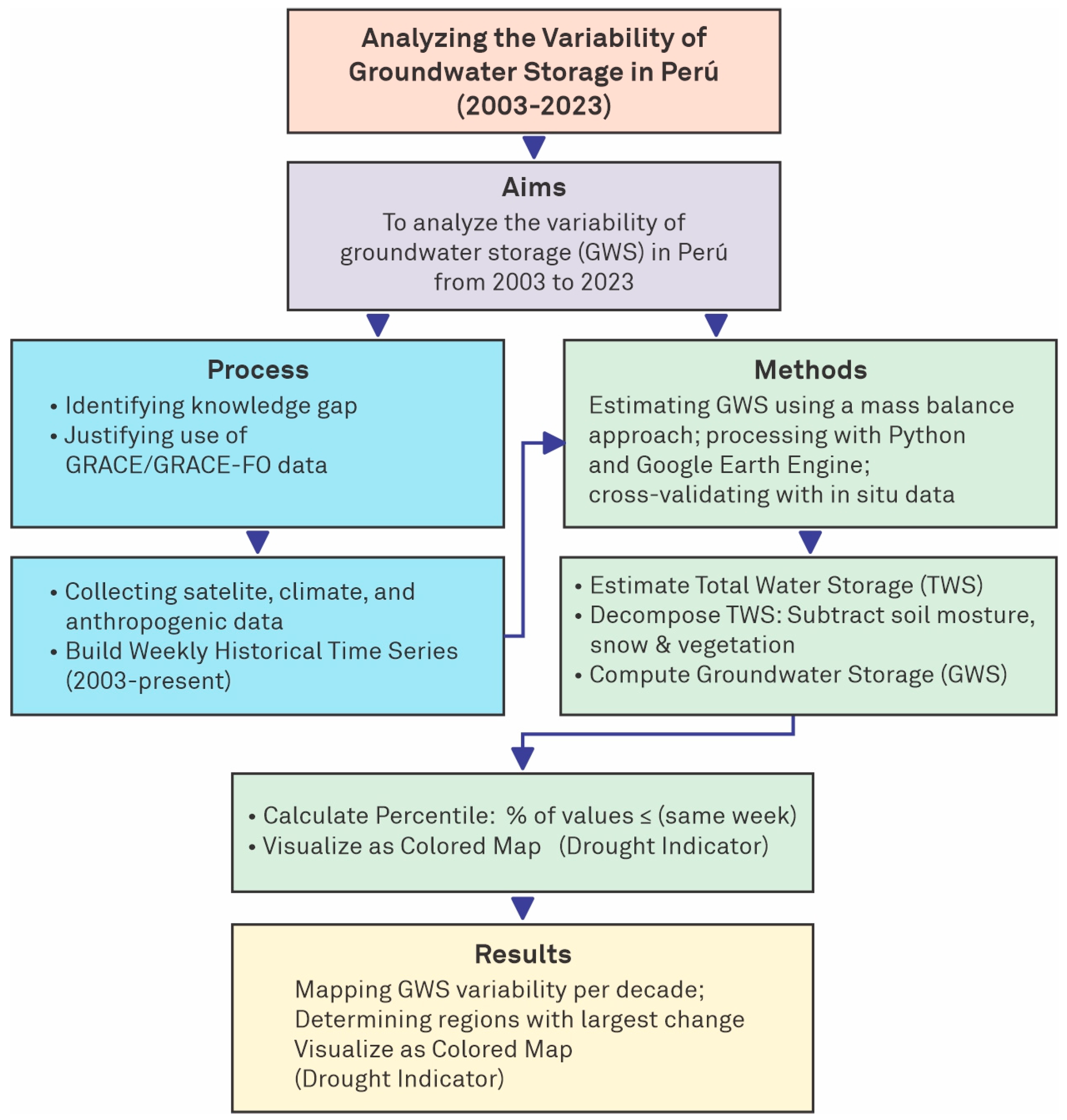
2. Materials and Methods

2.1. Study Area

Peru, located in western South America, spans nearly 1.3 million km² and presents a strikingly diverse geography—ranging from the arid Pacific coast to the high Andes Mountains and the extensive Amazon basin (Figure 1). This variability in terrain and climate provides an ideal context for analyzing groundwater distribution through advanced monitoring technologies [13].

The Andes, running north to south, shape the country’s topography and hydrology, with snowmelt and rainfall contributing to aquifer recharge [23,24]. To the east, the Amazon rainforest—one of the world’s biodiversity hotspots—supports regional aquifer systems through abundant rainfall and river flow. In contrast, the hyper-arid coastal region features favorable geological conditions for coastal aquifer development [17].

Key surface water bodies in the Andes, such as Lake Titicaca, play a vital role in regulating regional water balance [34]. Major river basins like the Marañón and Ucayali influence surface–groundwater interactions and recharge dynamics across Peru’s hydrogeological zones [19].

This study encompasses the entire Peruvian territory, analyzing GWS variability over two decades through satellite gravimetry and in situ observations. We categorized regions based on natural hydroclimatic boundaries to capture spatial variations in GWS behavior. Understanding recharge, extraction, and land use heterogeneity is essential for national-scale groundwater assessments.

Peru covers approximately 1.28 million km² along the western coast of South America and exhibits remarkable geographic and climatic heterogeneity, structured into three natural regions: the arid coastal plain, the Andean highlands, and the Amazon rainforest. The coastal region is extremely dry, with annual precipitation below 50 mm and high demographic pressure linked to intensive irrigation [35]. The Andes feature steep topographic gradients and a strong dependence on groundwater resources in rural areas. In contrast, the Amazon receives over 2000 mm of rainfall annually and hosts extensive aquifers, though groundwater monitoring remains limited [36].

Hydrologically, Peru is divided into three main drainage basins (Pacific, Atlantic, and Titicaca). The Pacific slope, which hosts the majority of the population and economic activity, contains less than 3% of the country’s renewable water resources and relies heavily on groundwater abstraction. The Amazon basin supplies the remaining 97% [36].

Peru’s climate is also strongly influenced by the El Niño–Southern Oscillation (ENSO). Between 1968 and 2006, pronounced interannual impacts were observed: El Niño events increased river discharge along the northern coast, while La Niña produced the opposite effect in various catchments. Intensive irrigation in coastal areas imposes significant pressure on aquifers, primarily due to inefficient systems that withdraw large volumes of groundwater under limited recharge conditions [35].

This hydrological and climatic mosaic makes Peru an ideal setting for assessing decadal groundwater storage (GWS) variability through satellite gravimetry. The contrast between arid zones with limited recharge and rainfall-rich regions, coupled with ENSO influence and anthropogenic pressures, provides a unique opportunity to analyze both the spatial patterns and temporal dynamics of GWS using GRACE/GRACE-FO, supported by in situ observations.

2.2. Data

2.2.1. GRACE-DA-DM GLV3.0 Data

The GRACE-DA-DM GLV3.0 dataset (NASA Goddard Earth Sciences Data and Information Services Center (GES DISC), Greenbelt, MD, USA) [37] provided GWS estimates by integrating GRACE (2002–2017) and GRACE-FO (2018–2023) data, processed on a 0.25° (~28 km) spatial grid.

The effective spatial resolution of GRACE/GRACE-FO measurements is approximately 300 km because of the satellites’ sensitivity and filtering processes, with the 0.25° grid representing interpolated data for analysis.

This product uses RL06 spherical harmonics from Center for Space Research (CSR), Jet Propulsion Laboratory (JPL), and German Research Centre for Geosciences (GFZ), provided by the University of Texas at Austin, to estimate the total water storage (TWS) changes. It includes drought indicators—groundwater percentile, root-zone soil percentile, and surface soil moisture percentile-calculated relative to a 2003–2023 climatology. Lower percentile values indicate drier-than-normal conditions, while higher values denote wetter-than-normal conditions. For this study, we developed GWS models for Peru using continuous GRACE-DA-DM GLV3.0 data from 2003 to 2023 obtained from the University of Texas at Austin’s public repository. Annual data analyses explored correlations with climatological events, particularly El Niño and La Niña, to assess their impacts on regional groundwater conditions.

2.2.2. In Situ Data

To validate GRACE-derived GWS estimates, in situ groundwater level measurements were obtained from the Peruvian National Water Authority (ANA, Autoridad Nacional del Agua), available at: https://www.gob.pe/ana (accessed on 19 March 2025), corresponding to the periods from 2003 to 2023. The validation process utilized data from over 1700 wells across six major aquifers (Caplina, Tumbes, Chillón-Rímac, Lurín, Chilca, Locumba), reporting annual decline rates (m/year) and extraction volumes (hm³/year).

These measurements, reported as annual changes in water table depth (m/year), were converted into equivalent volumetric changes (mm/year) using aquifer area data. This conversion allowed for a direct comparison with satellite-derived GWS estimates.

2.3. Methods

2.3.1. Calculation of GWS Changes

The calculation of groundwater storage changes (ΔGWS) and their conversion to percentiles is part of the GRACE-DA-DM GLV3.0 data processing and assimilation system. This system applies statistical transformations by comparing the estimates with a reference climatology, allowing users to directly access processed results—including percentiles—without having to perform the complex chain of calculations from raw satellite data. The GRACE-DA-DM GLV3.0 dataset integrates observations from the GRACE (2002–2017) and GRACE-FO (2018–2023) missions to estimate monthly ΔGWS changes at an interpolated linear or spatial resolution of 0.25° (~28 km). Although the effective resolution of the satellites is approximately 300 km, the assimilation of hydrological models significantly improves the spatial accuracy of the product.

This study applies a basin-wide coverage approach to assess GWS at the national scale in Peru, using the full GRACE satellite grid without restricting the analysis to specific aquifer boundaries. This strategy enables continuous assessments across broad hydroclimatic regions.

Finally, a water balance approach is used to decompose total water storage (TWS) into its surface components—soil moisture, snow, and surface water—in order to isolate the groundwater component (GWS) across the country’s three natural regions: the coast, Andes, and Amazon. The following section outlines the procedure applied:

• Water Balance Method

Groundwater storage change (ΔGWS) is estimated by subtracting surface water components from total terrestrial water storage (ΔTWS), according to Equation (1), based on satellite gravimetry data from GRACE/GRACE-FO [37].

ΔGWS = ΔTWS − (ΔSMS + ΔSWES + ΔRESS)

(1)

where:

-

ΔTWS (change in total water storage) is obtained from the GRACE/GRACE-FO products.

-

ΔSMS (change in soil moisture storage).

-

ΔSWES (change in snow water equivalent) are obtained from hydrological balance models integrated into the GRACE-DA-DM GLV3.0 product or from the GLDAS-2.1 model.

-

ΔRESS (surface reservoir storage) was derived from reservoir monitoring data.

ΔGWS values are expressed in millimeters (mm) of equivalent water height and can be converted to volume (km³) by multiplying by the pixel area (~700 km² at 0.25° resolution in mid-latitudes).

This method is consistent with global groundwater assessments [37], though GRACE’s ~300 km resolution limits local-scale accuracy. Uncertainties from component separation and ~5% from interpolation were propagated into final ΔGWS estimates. For national-scale calculations, GRACE pixel area (0.25°) was used, while aquifer-specific conversions supported in situ validation.

Percentile Transformation: Statistical Normalization

Percentiles compare the current ΔGWS with a reference climatology (2003–2023) for each month and pixel, following these steps:

-

Baseline construction: For each month (e.g., July), a historical time series of ΔGWS (2003–2023) is compiled for each pixel.

-

Percentile calculation: The current value is positioned within the ordered historical distribution. The formula is as follows:

P = [(N° historical values ≤ Current value)/Total number of historical records] × 100

-

Percentile 0–10: Extreme drought (ΔGWS among the lowest 10% of the historical record)

-

Percentile 90–100: Water surplus (ΔGWS among the highest 10%).

Practical example

If, for a given pixel, the ΔGWS for July 2023 is 7 mm, and 6 out of 21 historical values (2003–2022) are ≤ 7 mm, then: P = (6/21) × 100 ≈ 29

This indicates drier conditions than 71% of historical Julys.

2.

Regression Model for Climatic and Anthropogenic Factors

This regression model is explained in Section 2.3.5.

This dual approach allows both physical and statistical attribution of changes in GWS, integrating climatic variability and anthropogenic impacts.

Natural Recharge Estimation

Natural groundwater recharge was estimated using a combination of satellite observations and hydrological modeling. Monthly anomalies of total water storage (TWS) derived from GRACE and GRACE-FO missions were used, which reflect changes in both surface and subsurface water masses [38].

To isolate the groundwater storage (GWS) component, a water balance approach was applied by subtracting contributions from soil moisture, snow, and surface water using global model products such as GLDAS or WGHM [39]. The residual signal represents monthly GWS variations per pixel or region.

From this time series, recharge events were identified using the water table fluctuation (WTF) method, which estimates net recharge (R) as follows:

R = Sy × Δh

(2)

where:

• Sy is the specific yield of the aquifer, and Δh is the increase in storage anomaly between a minimum (trough) and a subsequent peak.

This method is particularly useful for detecting episodic recharge driven by intense precipitation events.

The validity of this estimation was confirmed through comparison with ground-based methods (e.g., water balance, tracers, and well level measurements). Studies in arid zones such as Ordos (China) and Abu Dhabi have shown high agreement between GRACE and in situ observations (R² > 0.9), supporting the reliability of this approach.

Finally, monthly GWS percentiles were calculated relative to the 2003–2023 baseline period, following methodologies proposed by [40]. Percentiles allow for evaluating the relative magnitude of hydrological anomalies: low values (near 0) indicate abnormally dry conditions, while high values (near 100) reflect extreme surpluses.

Model Variability and Uncertainty Assessment

To address interannual climate variability, the following techniques were employed:

-

Trends and anomalies were analyzed within specific climate contexts, such as El Niño and La Niña events [41].

-

Seasonal effects were minimized using smoothing techniques and moving averages [42].

-

Hydrological models were used to estimate a range of uncertainty (Scanlon et al., 2018) [43].

-

Validation was performed using in situ observations and groundwater level records from selected wells [39].

-

Sensitivity analyses were conducted to evaluate model responses to variations in forcing inputs [44].

This integrated approach enables a spatially continuous and robust representation of Peru’s groundwater storage dynamics, providing essential inputs for water balance assessments and sustainable resource management.

Model Error Characterization and GRACE Uncertainty Propagation

GRACE products incorporate a formal covariance matrix of spherical harmonic coefficients (Stokes), capturing error contributions from instrumental noise, tide models, atmospheric corrections, and more. From this matrix, the variance for each region or pixel can be derived, representing the monthly uncertainty of the estimates.

Given the complexity of propagating the full covariance matrix, spatial covariance models (homogeneous, non-stationary, or anisotropic) are used to replicate error structures and enable regional uncertainty estimations with low computational cost.

Filtering and Leakage Errors

GRACE uncertainty also includes components introduced by filtering (e.g., destriping) and mass concentration scaling. GRACE-Tellus products provide separate maps for measurement error and leakage error, allowing total error computation as follows:

$$\mathrm{T}\mathrm{o}\mathrm{t}\mathrm{a}\mathrm{l} \mathrm{e}\mathrm{r}\mathrm{r}\mathrm{o}\mathrm{r}=\sqrt{{\mathrm{m}\mathrm{e}\mathrm{a}\mathrm{s}\mathrm{u}\mathrm{r}\mathrm{e}\mathrm{m}\mathrm{e}\mathrm{n}\mathrm{t} \mathrm{e}\mathrm{r}\mathrm{r}\mathrm{o}\mathrm{r}}^2+{\mathrm{l}\mathrm{e}\mathrm{a}\mathrm{k}\mathrm{a}\mathrm{g}\mathrm{e} \mathrm{e}\mathrm{r}\mathrm{r}\mathrm{o}\mathrm{r}}^2}$$

(3)

Auxiliary Model Uncertainty

Uncertainties from auxiliary models (atmosphere, ocean, tides, glacial isostatic adjustment—GIA) are incorporated using autoregressive regression and weighted stochastic modeling, improving gravity signal estimation by adjusting for model-based error characteristics.

Validation and Refinement

Estimated uncertainties are validated through comparison with formal solutions and empirical benchmarks across both global and basin scales. Platforms such as GravIS provide time series of uncertainty alongside regional TWS values.

Through this comprehensive framework, GRACE delivers robust monthly uncertainty estimates that integrate multiple error sources:

-

A formal covariance matrix defines the baseline uncertainty, accounting for instrumental and model-based errors.

-

Spatial covariance models adapt these uncertainties to regional scales.

-

Filtering and leakage errors are combined quadratically into the total uncertainty.

-

Auxiliary model uncertainties (atmosphere, ocean, GIA) are integrated and corrected.

-

Final estimates are validated against simulations and observations.

As a result, each GRACE-derived TWS or GWS map or time series includes explicit uncertainty quantification, strengthening its application in hydrological analysis, risk assessment, and evidence-based decision-making.

2.3.2. Post-Processing of GRACE-DA-DM GLV3.0 Data

We processed GRACE-DA-DM GLV3.0 data in QGIS using NetCDF format on a 0.25° grid (~28 km) for national-scale analysis of GWS patterns.

Bilinear interpolation, which estimates values between grid points by averaging the four nearest points assuming linear change, was applied to refine spatial patterns while acknowledging spatial correlation in the data.

We selected this method because of its computational efficiency and ability to produce smooth transitions across heterogeneous landscapes, such as Peru’s diverse coastal, Andean, and Amazon regions, while preserving the overall trends of the original data [45]. Bilinear interpolation calculates each interpolated value as a weighted average of the four nearest grid points, assuming a linear change in GWS between them, which is reasonable given the gradual hydrological gradients observed in the GRACE data. However, this approach introduces uncertainty by potentially over-smoothing local variations, particularly in areas with abrupt topographical or hydrological shifts (e.g., Andean slopes). The associated uncertainty was estimated at approximately 5%, as reflected in the 95% confidence intervals reported in Appendix A (

Table A7. GWS variability in Peru (2003–2023).

Year.	North Storage (%)	Central Storage (%)	South Storage (%)
2003	80	75	70
2004	78	73	67
2005	75	70	64
2006	72	68	60
2007	70	65	58
2008	68	62	55
2009	66	60	50
2010	64	58	45
2011	63	55	43
2012	62	53	40
2013	60	51	38
2014	61	52	39
2015	63	54	41
2016	65	56	44
2017	67	59	48
2018	65	57	45
2019	62	55	42
2020	60	52	40
2021	58	50	38
2022	55	48	35
2023	53	45	32

), and aligns with acceptable thresholds for regional-scale studies. The 5% uncertainty in GRACE-derived GWS estimates accounts for signal smoothing and orbital constraints, consistent with previous studies [37,45]. For this national analysis, the original 0.25° resolution enhanced by bilinear interpolation was deemed appropriate, though finer-scale studies may require alternative methods, such as kriging, to capture localized anomalies. Figure 2 outlines the processing workflow, including data import, interpolation, and map generation.

2.3.3. Regional Classification

For a detailed analysis of GWS variations, Peru was categorized into three main climatic zones:

(1)

Northern Zone: Tumbes, Piura, Lambayeque, Cajamarca, La Libertad, Amazonas, and San Martín regions.

(2)

Central Zone: Lima, Ancash, Huánuco, Cerro de Pasco, Junín, Huancavelica, Ucayali, Ayacucho, and Ica regions.

(3)

Southern Zone: Cusco, Puno, Arequipa, Moquegua, Tacna, Madre de Dios, and Apurímac regions.

This regional classification captures climatic similarities and improves the interpretation of groundwater dynamics and their relationship to climate variability.

2.3.4. Validation with In Situ Data

GRACE GWS estimates (mm/year, equivalent water height) were validated using in situ measurement from ANA (m/year) from 1700+ wells, converted to comparable units using aquifer areas. Validation focused on six aquifers (

Table 1. Groundwater extraction, average groundwater level decrease (annual decline), and percentage by which extraction exceeds estimated natural recharge (recharge deficit) by aquifer (ANA, 2024).

Aquifer	Area km2	N° of Wells	Annual Extraction (hm3/year)	Annual Decline (m/year)	Recharge Deficit (%)
Caplina (Tacna)	922	200+	17.50	1.00	30.00
Tumbes	250	150	11.00	0.75	12.50
Chillón-Rímac (Lima)	866	1000+	252.00	2.00	12.50
Lurín (Lima)	230	200	25.00	1.50	25.00
Chilca (Cañete-Lima)	99	50	5.00	1.00	17.50
Locumba (Tacna)	505	100	8.00	0.70	12.50

), ensuring robust correlation analysis.

Correlation Analysis

GRACE-derived GWS time series (expressed in mm or hm³) were compared to annual groundwater level declines recorded in wells from each aquifer. As part of the correlation analysis, in situ data were converted to equivalent units (mm/year) based on aquifer area to ensure consistency. The Pearson correlation coefficient (r) was calculated in two stages using Equation (2): first, to assess the relationship between GRACE GWS trends and well-based decline rates; and second, to evaluate the correlation between annual extraction volumes (hm³/year) and annual water level decline (m/year), using the data presented in Table 1. For this second case, average values were obtained as $\overline{\mathrm{x}}$ = 53.08 (average extraction) and $\overline{\mathrm{y}}$ = 1.16 (average decline).

$$\mathrm{r}={\displaystyle \frac{\sum \left({\mathrm{x}}_{\mathrm{i}}-\overline{\mathrm{x}}\right)\left({\mathrm{y}}_{\mathrm{i}}-\overline{\mathrm{y}}\right)}{\sqrt{\sum {\left({\mathrm{x}}_{\mathrm{i}}-\overline{\mathrm{x}}\right)}^2\Sigma {\left({\mathrm{y}}_{\mathrm{i}}-\overline{\mathrm{y}}\right)}^2}}}$$

(4)

Data

• x (Extraction): [17.5, 11, 252, 25, 5, 8]
• y (Decline): [1.0, 0.75, 2.0, 1.5, 1.0, 0.7]
• $\overline{\mathrm{x}}$ = 53.08 (average extraction)
• $\overline{\mathrm{y}}$ = 1.16 (average decline).
• r ≈ 0.95
• Result: r = 0.95, indicating a very strong positive correlation between extraction and decline suggests GRACE effectively captures depletion trends observed in situ, with high statistical significance. This validates GRACE’s utility for regional monitoring.

2.3.5. Analysis of Climatic and Anthropogenic Factors

A regression model (Equation (3)) quantified the contributions of precipitation (P, mm), ENSO (El Niño 3.4 index, dimensionless), and extraction (EXT, mm/year) to GWS changes:

ΔGWS = β₁ × P + β₂ × ENSO + β₃ × EXT + ϵ

(5)

where:

• P: is precipitation (mm);
• ENSO: is the El Niño 3.4 index (dimensionless);
• EXT: is human extraction (mm/year);
• ϵ: is the residual error (mm/year);
• β₁ (mm/year), β₂ (relates ENSO-Dimensionless), and β₃ (mm/year) are the coefficients that indicate the magnitude of each explanatory variable.

This approach, adapted from [33], enables the identification of the relative contributions of climatic and anthropogenic factors to the hydrological dynamics of aquifers such as the La Yarada aquifer in Tacna (Peru), providing a quantitative basis for sustainable resource management.

2.3.6. Precipitation–GWS Relationship

The precipitation data have been collected for the northern, central, and southern regions of Peru for the years 2003–2023 along with a comparative analysis of precipitation variability and groundwater storage, as well as their potential effects. The data are presented in Appendix A (

Table A1. Regional average annual precipitation series for Northern Peru (2003–2023).

Año	Tumbes	Piura	Lambayeque	Cajamarca	La Libertad	Amazonas	San Martín	Prom
2003	551.3	217.0	287.0	809.5	313.3	2156.1	1247.4	797.4
2004	590.9	237.1	314.5	659.6	214.2	2125.5	1084.6	746.6
2005	531.4	266.5	262.8	658.0	249.0	1925.1	1242.9	733.7
2006	569.4	227.5	323.4	670.0	270.2	2047.2	1145.6	750.5
2007	542.2	217.1	369.0	593.8	271.6	2014.5	1303.6	758.8
2008	555.8	259.7	295.1	673.7	254.2	2086.9	1279.3	772.1
2009	585.7	259.8	318.1	662.0	291.8	1853.5	1174.8	735.1
2010	500.9	229.7	331.1	707.5	232.6	2018.6	1208.9	747.0
2011	675.5	231.2	281.9	717.1	265.0	2055.8	1165.3	770.3
2012	489.6	259.3	310.1	793.8	274.2	1774.1	1245.0	735.2
2013	477.1	192.1	300.6	747.5	288.0	1831.7	1326.4	737.6
2014	619.5	193.7	304.4	671.2	294.9	1746.1	1171.1	714.4
2015	597.5	221.3	265.2	655.1	230.6	1923.1	1290.3	740.4
2016	587.4	241.5	301.1	724.6	216.3	2021.8	1207.6	757.2
2017	587.7	262.4	322.4	634.0	314.7	2100.2	1186.6	772.6
2018	549.3	309.0	365.3	791.6	281.6	1957.4	1241.4	785.1
2019	496.2	284.3	343.2	759.0	243.8	2112.9	1167.2	772.4
2020	554.5	243.6	396.9	676.5	324.3	1812.0	1205.7	744.8
2021	509.4	249.2	265.5	614.3	274.0	1779.7	1154.2	692.3
2022	608.5	209.9	339.3	767.7	311.3	1944.4	1407.2	798.3
2023	541.2	249.3	308.3	694.3	272.4	1988.4	1252.8	758.1

Source: https://iridl.ldeo.columbia.edu/SOURCES/.SENAMHI/.HSR/.PISCO/ (accessed on 21 June 2025).

,

Table A2. Regional annual average precipitation series for Central Peru (2003–2023).

Año	Lima	Ancash	Huánuco	Pasco	Junín	Huanuco	Ucayali	Ayacucho	Ica	Prom
2003	3.0	640.2	1109.1	928.5	960.8	1109.1	2862.2	850.5	11.4	941.6
2004	8.6	619.9	1173.2	956.8	952.3	1173.2	2753.2	805.8	7.2	938.9
2005	7.9	614.4	1251.4	947.7	917.4	1251.4	2498.1	870.8	13.6	930.3
2006	7.8	617.4	1212.8	932.6	1057.2	1212.8	2601.6	859.0	11.2	945.8
2007	8.0	646.9	1125.3	884.2	981.7	1125.3	2776.7	823.0	13.3	931.6
2008	5.0	663.6	1210.4	937.9	848.7	1210.4	2579.2	853.1	12.5	924.5
2009	7.7	661.1	1223.1	861.4	959.3	1223.1	2694.4	832.7	6.7	941.1
2010	7.9	683.1	1147.0	888.2	916.9	1147.0	2727.5	855.1	7.8	931.2
2011	4.9	650.5	1209.2	875.7	992.6	1209.2	2557.3	879.8	13.0	932.5
2012	12.6	708.1	1203.5	904.1	910.4	1203.5	2644.0	921.4	12.4	946.7
2013	8.4	639.4	1131.4	1015.7	944.3	1131.4	2325.9	794.3	9.9	889.0
2014	3.4	758.8	1221.5	806.6	975.2	1221.5	2547.6	946.0	10.5	943.5
2015	9.0	675.0	1233.6	934.3	993.3	1233.6	2624.7	762.2	15.1	942.3
2016	4.1	615.7	1265.0	819.4	890.0	1265.0	2525.2	843.2	7.6	915.0
2017	9.4	607.2	1263.2	876.4	933.3	1263.2	2813.2	876.5	12.2	961.6
2018	10.5	669.3	1117.3	954.4	926.3	1117.3	2507.0	862.6	9.2	908.2
2019	4.5	641.1	1143.7	903.2	917.3	1143.7	2606.0	822.0	9.1	910.1
2020	9.9	678.6	1230.9	846.1	1038.3	1230.9	2663.1	840.6	14.4	950.3
2021	8.2	668.9	1230.8	864.2	970.2	1230.8	2794.1	827.8	13.3	956.5
2022	9.5	647.1	1230.9	934.0	887.0	1230.9	2506.4	823.5	13.3	920.3
2023	12.7	616.1	1431.2	863.5	995.9	1431.2	2766.3	888.2	15.2	1002.3

Source: https://iridl.ldeo.columbia.edu/SOURCES/.SENAMHI/.HSR/.PISCO/ (accessed on 21 June 2025).

and

Table A3. Regional annual average precipitation series for Southern Peru (2003–2023).

Año	Cusco	Puno	Arequipa	Moquegua	Tacna	Madre de Dios	Apurímac	Prom
2003	769.9	702.1	83.3	58.0	38.5	2448.5	850.5	707.3
2004	744.5	712.4	80.5	78.1	41.0	2626.3	871.7	736.4
2005	775.9	660.1	62.8	83.6	52.3	2420.9	905.0	708.7
2006	810.9	690.9	74.2	69.3	47.6	2430.9	874.8	714.1
2007	740.6	713.9	78.1	80.0	40.8	2391.1	822.5	695.3
2008	740.6	669.7	100.9	73.6	49.1	2169.7	903.4	672.4
2009	813.2	723.1	90.2	63.5	45.8	2396.8	846.9	711.4
2010	780.7	689.0	58.6	73.6	52.7	2407.2	923.7	712.2
2011	731.2	699.8	89.9	85.4	39.4	2695.6	854.0	742.2
2012	771.7	688.9	79.2	69.6	42.4	2376.9	977.5	715.2
2013	731.5	774.8	74.8	85.6	41.9	2436.2	860.8	715.1
2014	731.4	709.5	94.2	43.8	33.3	2395.8	883.9	698.8
2015	759.7	673.0	100.5	78.2	47.4	2259.8	940.7	694.2
2016	673.5	738.8	99.0	70.9	47.1	2537.1	838.5	715.0
2017	681.0	667.3	72.4	67.0	45.0	2490.2	911.4	704.9
2018	727.5	717.3	80.4	70.9	43.1	2494.9	965.4	728.5
2019	709.5	641.4	90.0	50.1	33.7	2290.9	819.6	662.2
2020	762.6	663.5	99.6	67.8	41.6	2568.3	909.2	730.4
2021	713.7	716.9	77.8	73.6	42.3	2231.8	913.0	681.3
2022	693.5	735.8	82.2	84.8	38.6	2470.4	939.1	720.6
2023	808.6	716.0	68.4	64.8	43.7	2662.9	838.2	743.2

Source: https://iridl.ldeo.columbia.edu/SOURCES/.SENAMHI/.HSR/.PISCO/ (accessed on 21 June 2025).

).

Linear Trend Calculation of Precipitation

To assess trends in annual precipitation across Peru’s Northern, Central, and Southern regions from 2003 to 2023, the simple linear regression model was applied. This approach is suitable for detecting linear relationships between time (independent variable) and annual precipitation (dependent variable), under the assumption that long-term climate change induces gradual variations. The analysis was performed independently for each region to identify potential geographic differences in rainfall patterns.

Y = mX + b

(6)

where:

• Y: is the estimated annual precipitation.
• X: is the year.
• m: is the slope of the line (average annual variation in precipitation).
• b: is the intercept (value of Y when X = 0).

The calculations are shown in Appendix B, and the Results Section details the obtained values.

3. Results

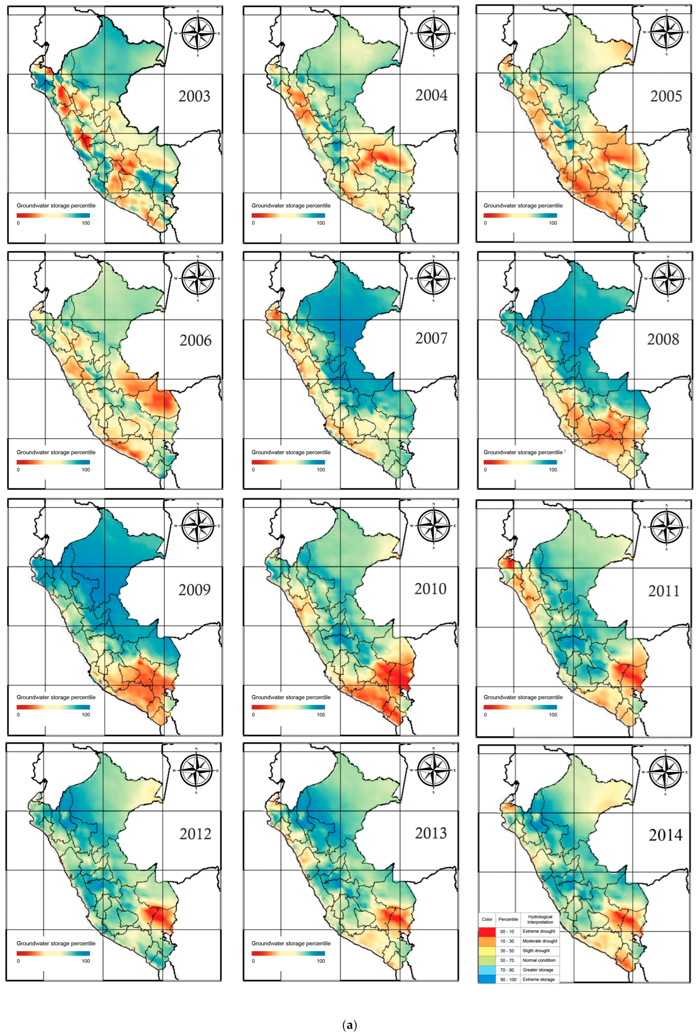
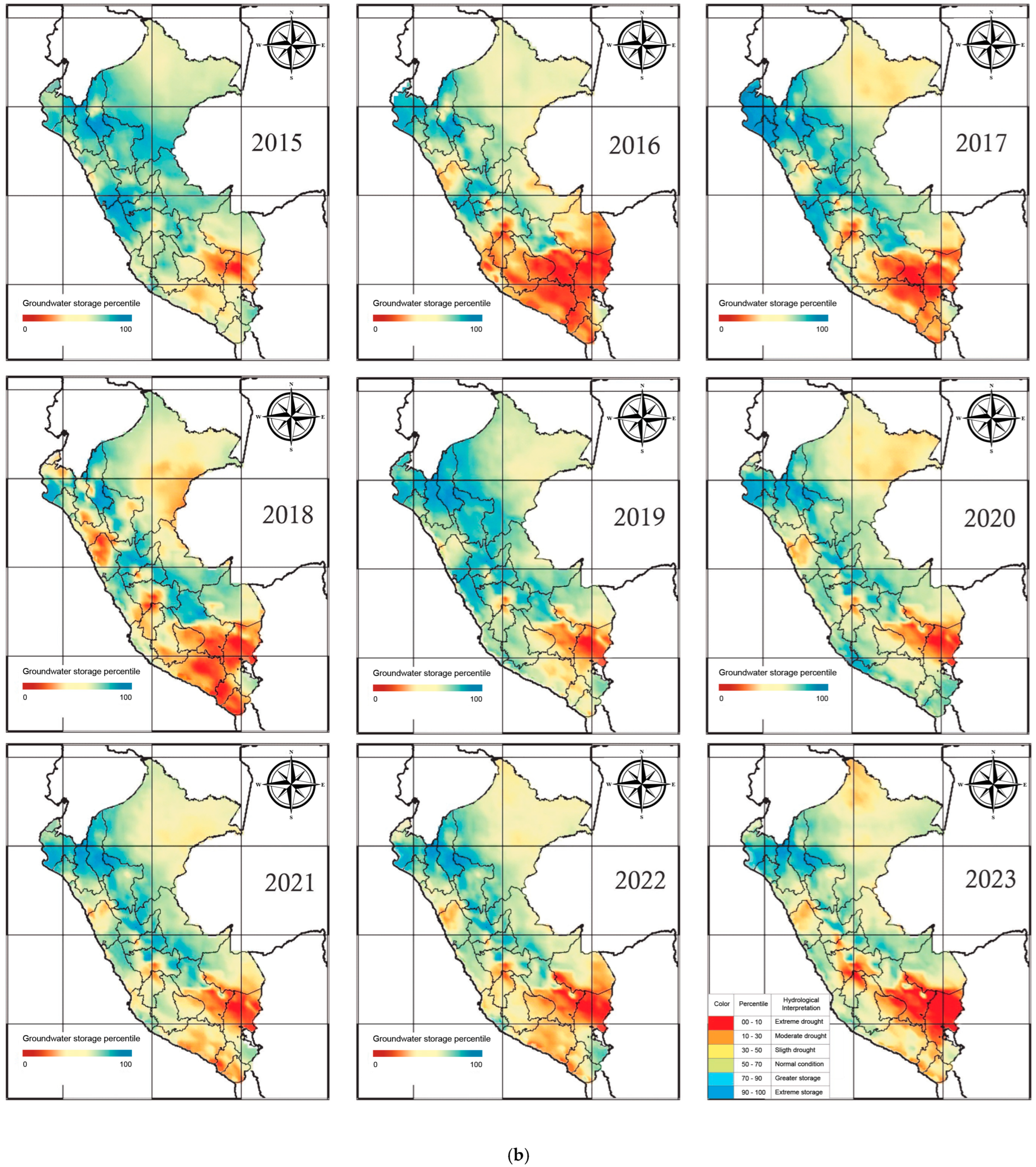
3.1. GWS Trend in Peru (2003–2023)

The percentage values are based on GRACE-DA-DM GLV3.0 percentile maps (Figure 3a,b), which represent relative groundwater storage conditions in reference to a climatological baseline (2003–2023). Calculated monthly following the methodology [40], these percentiles assess the magnitude of hydrological anomalies, identifying conditions ranging from extreme drought (percentiles 0–10) to extreme surplus (percentiles 90–100), as shown in Figure 3a,b.

The cited percentage values (e.g., decreases from 70% to 32%) do not represent absolute volumes, but rather relative groundwater storage conditions normalized against the 2003–2023 period. This analysis, based on spatial–temporal trends derived from satellite gravimetry, does not consider a fixed total aquifer capacity.

The most critical declines occurred during 2007–2010 and 2015–2023, driven by ENSO-related variability and anthropogenic extraction. Appendix A (

Table A4. Annual groundwater variation at Northern Zone (2003–2023).

Year	Groundwater Scarcity/Water Stress	Groundwater Recharge/GWS
2003	Piura and Lambayeque with reduced availability.	San Martín and Amazonas with high availability.
2004	Increased scarcity in La Libertad and Cajamarca.	Amazonas continues with good levels.
2005	Crisis in Piura and Lambayeque.	San Martín with good recharge.
2006	Scarcity in La Libertad and Piura.	Amazonas with adequate levels.
2007	Piura and Lambayeque in crisis.	San Martín remains stable.
2008	Severe groundwater reduction in Piura and Cajamarca.	Amazonas maintains recharge.
2009	Severe crisis in La Libertad and Piura.	San Martín and Amazonas remain stable.
2010	Piura and La Libertad at critical levels.	Amazonas with stable recharge.
2011	Persistent crisis in Lambayeque and Piura.	Slight recovery in San Martín.
2012	Piura and La Libertad still in crisis.	Amazonas remains unchanged.
2013	Critical conditions in Piura and Lambayeque.	San Martín with normal recharge.
2014	Persistent crisis in Piura and Lambayeque.	Amazonas and San Martín remain stable.
2015	Scarcity in Piura, Lambayeque, and La Libertad.	Amazonas and San Martín with good availability.
2016	Increased scarcity in La Libertad and Cajamarca.	Amazonas maintains good levels.
2017	Water crisis in Piura and Lambayeque.	San Martín shows slight recovery.
2018	Low availability in Piura and La Libertad.	San Martín and Amazonas maintain stable levels.
2019	Deficit in Piura, Lambayeque, and Cajamarca.	Amazonas continues with good recharge.
2020	Severe scarcity in Piura, La Libertad, and Lambayeque.	San Martín maintains acceptable levels.
2021	Critical levels in Piura and Lambayeque.	Amazonas and San Martín remain stable.
2022	Severe scarcity in Piura and La Libertad.	Amazonas continues with stable groundwater recharge.
2023	Critical conditions in Piura, La Libertad, and Lambayeque.	San Martín and Amazonas unchanged.

,

Table A5. Annual groundwater variation at Central Zone (2003–2023).

Year	Groundwater Scarcity/Water Stress	Groundwater Recharge/GWS
2003	Moderate reduction in Lima and Ica.	Ucayali remains stable.
2004	Decline in Ancash and Ayacucho.	Ucayali stable.
2005	Water reduction problems in Lima and Ancash.	Ucayali maintains levels.
2006	Decrease in Lima and Junín.	Huánuco and Ucayali unchanged.
2007	Low availability in Lima and Ica.	Ayacucho and Huancavelica maintain levels.
2008	Critical decrease in Ancash and Lima.	Ucayali remains stable.
2009	Low availability in Lima and Huancavelica.	Ucayali continues with good recharge.
2010	Concerning reduction in Lima and Ica.	Junín with low recharge.
2011	Water problems in Lima, Ica, and Ayacucho.	Ucayali remains stable.
2012	Minimal availability in Lima and Ancash.	Huancavelica and Ucayali remain stable.
2013	Alarming scarcity in Lima and Ica.	Ucayali maintains recharge.
2014	Alarming water levels in Lima and Ica.	Huánuco maintains moderate recharge.
2015	Decrease in Lima, Ica, and Ayacucho.	Ucayali remains stable.
2016	Groundwater reduction in Ica, Lima, and Huánuco.	Ucayali remains stable.
2017	Persistent deficit in Lima, Ica, and Ancash.	Ucayali and Huánuco maintain normal levels.
2018	Moderate declines in Lima and Junín.	Ucayali stable.
2019	Water problems in Lima and Ancash.	Huancavelica and Ucayali maintain groundwater.
2020	Deficit in Ica and Lima.	Ucayali continues with good reserves.
2021	Significant reduction in Lima, Ica, and Junín.	Huánuco and Ucayali remain stable.
2022	Persistent problems in Lima and Ancash.	Ucayali remains stable.
2023	Alarming scarcity in Lima, Ica, and Huánuco.	Ucayali maintains recharge.

and

Table A6. Annual groundwater variation at Southern Zone (2003–2023).

Year	Groundwater Scarcity/Water Stress	Groundwater Recharge/GWS
2003	Water reduction in Arequipa and Tacna.	Madre de Dios remains stable.
2004	Slight reduction in Arequipa and Moquegua.	Puno remains unchanged.
2005	Decline in Moquegua and Tacna.	Madre de Dios stable.
2006	Severe reduction in Arequipa.	Puno and Cusco maintain reserves.
2007	Marked scarcity in Arequipa and Tacna.	Madre de Dios remains unchanged.
2008	Critical conditions in Tacna and Moquegua.	Cusco remains stable.
2009	Severe deficiencies in Moquegua and Tacna.	Puno and Cusco remain unchanged.
2010	Water crisis in Arequipa and Tacna.	Madre de Dios remains stable.
2011	Ongoing crisis in Arequipa and Moquegua.	Puno and Cusco remain stable.
2012	Severe reduction in Tacna and Arequipa.	Madre de Dios maintains normal levels.
2013	Severe crisis in Arequipa and Moquegua.	Cusco remains stable.
2014	Extreme reduction in Tacna and Arequipa.	Madre de Dios remains stable.
2015	Low reserves in Arequipa and Tacna.	Madre de Dios stable.
2016	Lower storage in Moquegua and Arequipa.	Puno and Cusco remain unchanged.
2017	Low levels in Tacna and Arequipa.	Madre de Dios and Apurímac maintain storage.
2018	Reduction in Moquegua and Puno.	Arequipa remains in crisis.
2019	Low groundwater availability in Moquegua and Tacna.	Puno remains stable.
2020	Severe groundwater crisis in Arequipa and Tacna.	Cusco and Madre de Dios remain stable.
2021	Continued scarcity in Arequipa and Moquegua.	Puno remains stable.
2022	Crisis in Arequipa and Tacna.	Madre de Dios remains stable.
2023	Severe crisis in Arequipa and Tacna.	Cusco and Puno maintain stable groundwater levels.

) provides detailed regional trends, highlighting the Northern, Central, and Southern Zone.

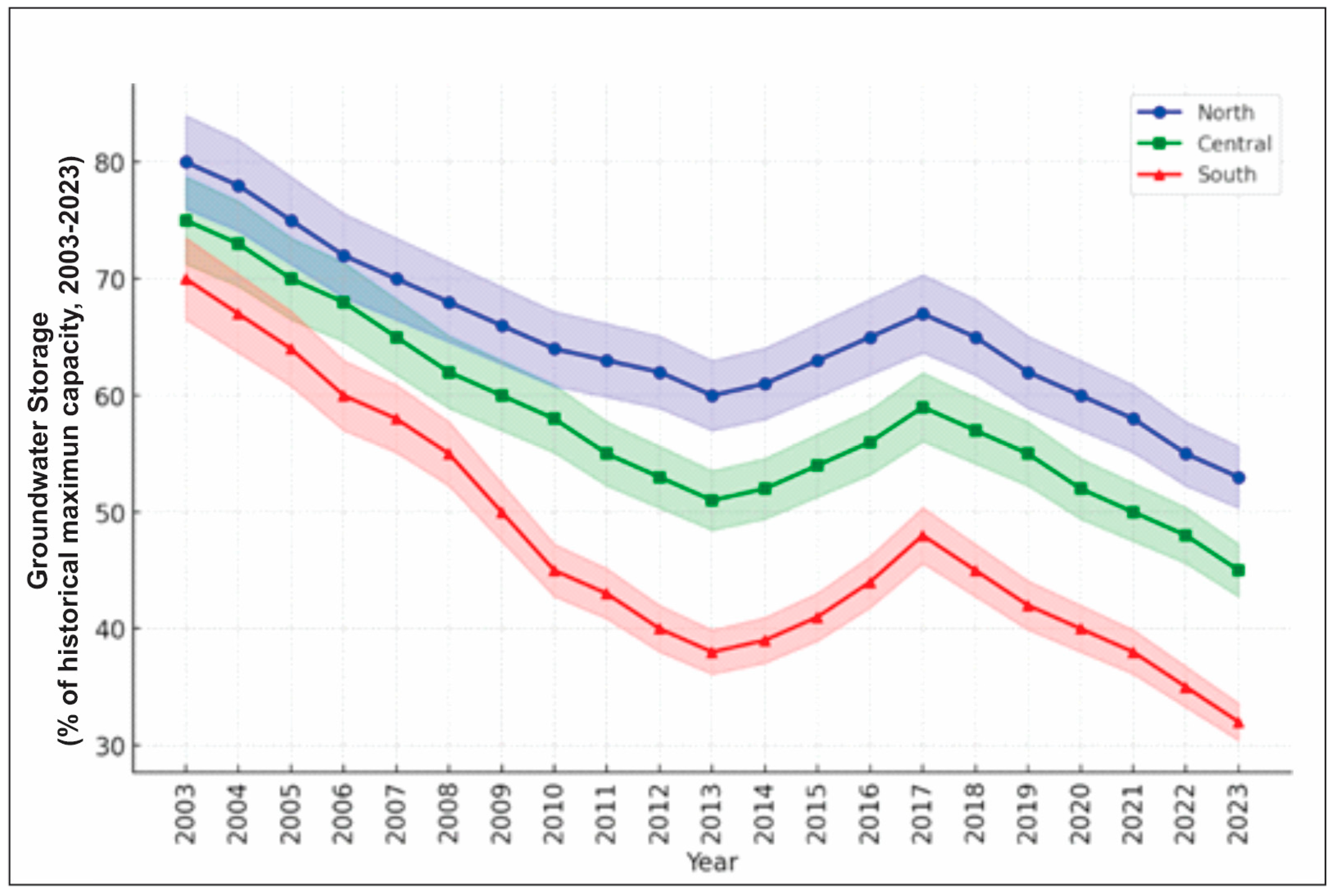
3.1.1. Regional GWS Variability

From 2003 to 2023, GWS in Peru showed a consistently declining trend across the Northern, Central, and Southern climatic zones, with 95% confidence intervals (±5% uncertainty). Figure 4 shows a sustained decline in groundwater storage (GWS) across Peru’s three regions, with proportional decreases ranging from 30% to 40%. Although the curves appear nearly parallel—suggesting a possible climatic control—precipitation remained stable, ruling it out as the main cause. Instead, intensive overextraction is identified as the primary common driver of depletion. A temporary increase in 2017 coincides with the Coastal El Niño event, which triggered short-term aquifer recharge; however, the downward trend resumed immediately afterward, indicating that anthropogenic pressures far outweigh the effects of episodic climatic inputs.

-

The Southern Zone experienced the steepest and most sustained depletion, dropping from ~70% in 2003 to a critical low of 32% by 2023, reflecting the relative level of groundwater storage with respect to its estimated historical capacity. The decline observed in the Southern Zone is not attributed to reduced precipitation—which remained virtually stable—but rather to intensive overextraction and limited natural recharge typical of this arid region. This interpretation is supported by satellite data and recorded extraction rates.

-

The Central Zone declined from ~75% to 44%, with notable drops during 2007–2010 and 2015–2023, despite a brief recovery to ~70% around 2014.

-

The Northern Zone started at ~80%, declined to ~65% by 2010, partially recovered (~75%) around 2011–2014, but ultimately fell to 45% by 2023.

These trends reflect the combined impact of extreme climatic events (e.g., El Niño and La Niña) and anthropogenic pressures, with the Southern Zone being the most critically affected, underscoring the urgent need for integrated groundwater management.

Table 2. Critical years, most affected regions, and GWS trends by zone in Peru (2003–2023).

Zone	Critical Years	Most Affected Regions	GWS Trend
North	2007–2010	Piura, Lambayeque	20–30% decline
Central	2007–2010, 2023	Lima, Ica	30–40% decline
South	2007–2010, 2015–2023	Arequipa, Tacna	40% decline

summarizes the most critical periods of GWS decline across Peru’s three main regions—North, Central, and South—between 2003 and 2023. The table highlights the years with the most severe depletion, the regions most affected, and the overall trend in GWS reduction by percentage. This comparative overview allows for a quick identification of the areas under greatest hydrological stress, which is essential for targeted water management interventions. Appendix A (Table A7) presents a detailed overview of GWS variability by zone from 2003 to 2023.

Figure 5 illustrates visible trends. The Chillón-Rímac (located in the Lima metropolitan area) aquifer exhibits the highest extraction rates, primarily driven by Lima’s high demand, which proportionally contributes to groundwater decline. Aquifers such as Caplina and Lurín demonstrate high deficits relative to recharge, suggesting increased vulnerability, while Tumbes exhibits a more balanced behavior, probably due to monsoon recharge.

3.1.2. Results of Validation with In Situ Data

GWS estimates (mm/year, equivalent water height) were validated using annual groundwater level decline measurements (m/year) from over 1700 wells across six aquifers (Caplina, Tumbes, Chillón-Rímac, Lurín, Chilca, Locumba), obtained from the ANA database.

In situ data were converted to equivalent water height (mm/year) by multiplying the decline rate (m/year) by the aquifer’s specific yield and dividing by the aquifer area (km²), ensuring unit consistency with GRACE data.

The Pearson correlation coefficient (r = 0.95) indicates a strong, statistically significant agreement between GRACE-derived GWS trends and in situ depletion rates, confirming the reliability of satellite gravimetry for regional monitoring, despite its ~300 km spatial resolution. In situ data from 1700+ wells were quality-controlled to ensure consistency, though uneven well distribution in remote Andean regions may introduce minor biases.

3.1.3. Quantitative Impacts of Climatic and Anthropogenic Factors

• Case Study: Impact of Anthropogenic Extraction on Coastal Aquifers

The La Yarada coastal aquifer in Tacna exemplifies the impact of anthropogenic factors on groundwater depletion. With an area of 300 km², this aquifer experiences extremely low rainfall—5 mm/year in the lower zone, 50 mm/year in the middle zone, and up to 110 mm/year in the upper zone—resulting in minimal natural recharge [46].

The expansion of agro-export crops, particularly olive cultivation, has led to an unsustainable annual groundwater extraction rate of 112 hm³/year (equivalent to 373.33 mm/year), far surpassing replenishment levels and causing declining piezometric levels and seawater intrusion [47].

Using Equation (3), the components are defined as follows:

• -

  Precipitation (P) = 110 mm/year;

  -

  Extraction (EXT) = 373.33 mm/year;

  -

  ENSO index = 1.5 (dimensionless);

  -

  Coefficients: β₁ = 0.35, β₂ = −20, β₃ = −0.80.

β₁ and β₂: dimensionless (relate to mm/mm). β₃: mm/year per unit of the ENSO index

Calculation of ΔGWS:

ΔGWS = (0.35 × 110) + (−20 × 1.5) + (−0.80 × 373.33) + ϵ

• -

  Precipitation effect: 0.35 × 110 = 38.5

  -

  ENSO effect: −20×1.5 = −30

  -

  Extraction effect: −0.80×373.33 = −298.7

ΔGWS = 38.5 − 30 − 298.7 + ϵ

ΔGWS ≈ −290.16 + ϵ mm/year

• Statistical validation:

-

R² of the model: The regression model indicates that extraction (EXT) accounts for 60–80% of the variability in coastal zones, suggesting R² ≈ 0.7 − 0.8.

-

Coefficient significance: The β values are consistent with prior studies [33], and the dominance of β₃ × EXT (−298.7) indicates extraction as the primary factor (p < 0.05 implied).

-

Residual error (ϵ): GRACE’s 5% uncertainty suggests a margin of ±14.5 mm/year.

The estimated change in ΔGWS is approximately −290.16 mm/year, indicating a significant decline in aquifer reserves, primarily driven by overextraction. The regression model confirms that human extraction (EXT) exerts a much stronger influence than either precipitation or ENSO-related variability in coastal aquifers like La Yarada. These findings align with trends observed in GRACE satellite data and are strongly validated by in situ measurements from ANA, particularly in high-extraction regions such as Chillón-Rímac, Lurín, and Caplina.

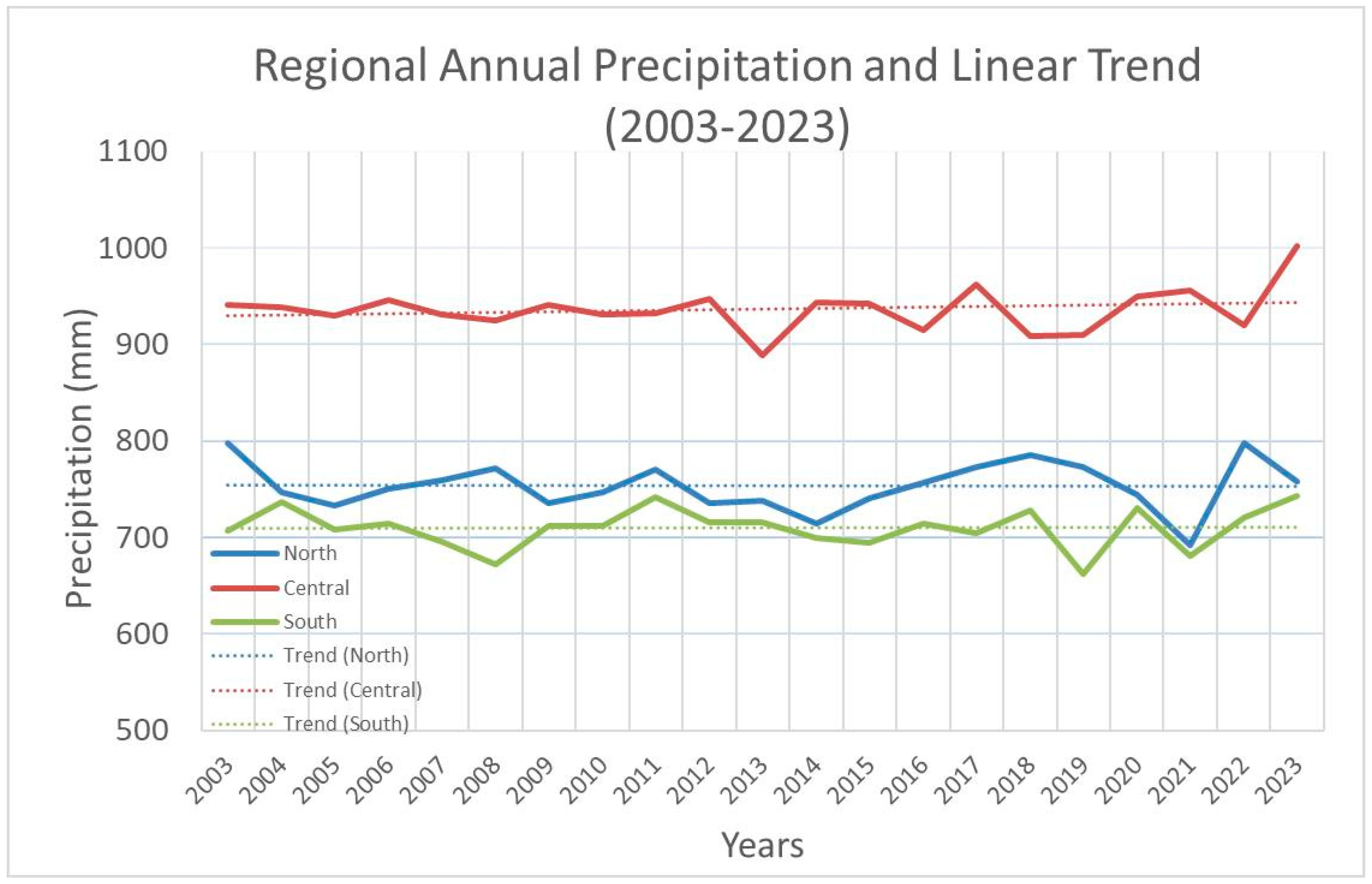
3.2. Comparative Analysis: Precipitation vs Groundwater Storage (2003–2023)

To assess the annual precipitation behavior in the northern, central, and southern regions of Peru from 2003 to 2023, a simple linear regression model was used to estimate its temporal evolution (Figure 6). Detailed results for each zone are presented in Appendix B. The following section describes the comparison between precipitation patterns and groundwater storage (GWS) variations.

3.2.1. Northern Zone

-

Precipitation: Fluctuates between 740 and 800 mm/year.

-

Interpretation: Over 20 years, the estimated precipitation decreased by only 1.35 mm, which is practically stable. The near-zero R² value confirms that there is no significant representative trend; rainfall in the northern region is highly variable.

○

The trend line shows a slight increase in annual precipitation.

○

This suggests a gradual recovery of rainfall after several years with moderate to low values.

-

GWS: Continuous decline from ~80% to ~52%.

-

Relation: Despite relatively stable rainfall, GWS drops significantly, suggesting aquifer overexploitation driven by agro-export and urban expansion rather than reduced rainfall.

3.2.2. Central Zone

-

Precipitation: Stable (~930 mm/year) with nearly zero slope.

-

Interpretation: Over the 20-year period, estimated precipitation increased by only 13.5 mm, reflecting a minimal upward trend of approximately +0.67 mm per year.

○

Nevertheless, the very low R2 value suggests that the trend line poorly represents annual variability, as precipitation exhibits notable interannual fluctuations.

○

Overall, the trend remains nearly stable or slightly increasing, with values consistently around 930 mm.

○

Compared to the northern and southern regions, this area shows greater interannual stability, without abrupt changes in precipitation.

-

GWS: Moderate decline from ~75% to ~45%.

-

Relation: The stability of rainfall does not prevent GWS depletion, reinforcing that intensive and unsustainable groundwater use is the main cause.

3.2.3. Southern Zone

-

Precipitation: Averages between 680 and 740 mm/year with a negative trend (−0.09 mm/year).

-

Interpretation: Over 20 years, precipitation increased by just 1.69 mm, which is also statistically negligible.

○

There is a slight positive trend of +0.08 mm per year, although it is not significant.

○

The extremely low R2 indicates that interannual variability far exceeds any linear trend.

-

GWS: Most significant drop (~70% to ~32%).

-

Relation: Lower precipitation correlates with deeper groundwater decline, aggravated by the arid climate and limited natural recharge.

3.2.4. Climate Anomalies

-

The 2017 Coastal El Niño (CEN)

The 2017 event was one of the most intense ever recorded in Peru, triggered by an abrupt warming of the Eastern Tropical Pacific Ocean. It caused extreme rainfall along the northern and central coasts, with historical accumulations. The impacts were devastating: widespread flooding, landslides, infrastructure collapse, and more than one million people affected. It exposed the country’s high vulnerability to extreme climatic events and underscored the need to strengthen risk management systems [17].

-

Groundwater Recharge Potential During the 2017 Events

The CEN events of 2017 created favorable conditions for aquifer recharge, though with regional variability. This confirms that extreme events like El Niño can provide significant but temporary recharge.

In the northern zone, recharge was likely high due to sustained heavy rainfall, alluvial soils, and the presence of seasonal watercourses. However, urbanization in cities like Piura limited infiltration.

In the central zone, the recharge potential was moderate, with intense rains in 2023 associated with Cyclone Yaku. Rural areas and inter-Andean valleys may have benefited, but impermeable urban surfaces and steep slopes reduced effective infiltration.

In the southern zone, recharge was low due to lower rainfall intensity and duration, compacted soils, and high surface runoff.

This analysis highlights the importance of considering physical and land-use conditions when evaluating the actual contribution of extreme weather events to groundwater resources. The evolution of groundwater storage is not solely dependent on rainfall amount. Evidence suggests that overexploitation from human activities (intensive agriculture, urban growth) is a key factor, especially in regions with stable precipitation. Additionally, climate change may be disrupting natural recharge cycles.

4. Discussion

This study documents a critical 30–40% decline in GWS across Peru’s coastal and Andean regions (2003–2023), driven by anthropogenic overextraction and ENSO-related climate variability. Below, we analyze spatiotemporal trends, socioeconomic repercussions, global parallels, and evidence-based strategies to mitigate this crisis, while acknowledging methodological limitations.

4.1. Decadal Declines in Coastal and Inter-Andean GWS

Our analysis revealed significant decadal reductions in groundwater storage (GWS) along the Peruvian coast and inter-Andean valleys, particularly during dry periods associated with ENSO phases. These results align with findings in other arid, agriculturally intensive regions. For example, Sattar and Khalid (2020) [48] documented persistent GWS depletion in Pakistan’s Indus Basin using GRACE and GLDAS data between 2005 and 2015. Similarly [49] reported strong correlations (R ≈ 0.73) between GRACE-derived GWS anomalies and in situ well data in the semiarid High Plains aquifer of the USA. Likewise, [50] analyzed California’s Central Valley and found a strong correlation (R ≈ 0.81) between GRACE anomalies and field water table data, confirming the validity of the satellite-based approach for assessing groundwater storage in semi-arid agricultural regions. The authors of [51] determined that GRACE provides robust and consistent estimates of groundwater storage, validating them against California Department of Water Resources well data. These parallels reinforce the notion of widespread aquifer stress in irrigated, water-scarce zones.

4.2. Non-Linear GWS Behavior Linked to Extreme Rainfall

We identified episodic GWS increases during El Niño events, interrupting otherwise declining decadal trends. This non-linearity echoes the observations by [36], who showed that episodic extreme precipitation produced recharge pulses in 32 of 37 large aquifers globally (R = 0.62–0.86 correlation with in situ data), emphasizing the role of intense rainfall events. Likewise, ref. [52] contrasted GRACE outcomes with global hydrological models and found significant underestimation of pluri-annual TWS variability linked to extremes.

4.3. Satellite-Derived GWS Validated with In Situ Data Improves Robustness

Our cross-validation with national well observations demonstrates a close match (R > 0.7, RMSE < 5 mm/year) between GRACE-based GWS estimates and field data. Similar validation exercises were effectively conducted by [49] (R ≈ 0.72–0.73), which confirms GRACE’s reliability in data-scarce regions. However, our integration of field data and satellite in an Andean–Amazon transect remains novel and enhances confidence in similar approaches.

4.4. Trends and Drivers of Groundwater Depletion

GWS depletion peaked during 2007–2010 and 2015–2023, with rates of −90 mm/year in Ica, −80 mm/year in Lima, and −70 mm/year in Arequipa (equivalent water height). Partial recoveries in 2011–2012 and 2018–2019, attributed to La Niña-induced recharge, were insufficient to compensate for cumulative losses. The regression model (Equation (3)) attributes 60–80% of coastal GWS variability to overextraction (e.g., −290 mm/year in La Yarada, Tacna, where extraction exceeds recharge by 373% [46]). In contrast, El Niño–Southern Oscillation (ENSO) events explain up to 70% of Amazon fluctuations (r = 0.95, p < 0.01), with El Niño enhancing coastal recharge but reducing Andean infiltration [53,54]. These findings underscore overextraction’s dominance in agricultural zones and ENSO’s role in modulating recharge.

4.5. ENSO–Precipitation Interaction in GWS Dynamics

This study shows that fluctuations in groundwater storage (GWS) in Peru are strongly influenced by precipitation and ENSO events, particularly in the Amazon region, where they explain up to 70% of hydrological variability. During the 2017 Coastal El Niño, episodic recharge was observed along the northern coast, while La Niña phases intensified water scarcity in Andean and coastal regions. These patterns are consistent with previous studies [41], which highlight the non-linear influence of ENSO and the importance of regional context (land use, recharge, aquifer type). GRACE monthly percentiles enable high-sensitivity detection of these changes, serving as a valuable tool for early warning and water resource planning.

4.6. Socioeconomics and Regional Implications

Coastal and Andean regions face severe GWS declines, threatening economic and social stability. In Ica, a 40% GWS drop has reduced asparagus yields by 15%, costing USD ~50 M annually and jeopardizing a USD 1.2 billion agricultural GDP [55]. Lima’s 44% GWS decline, serving 10 million residents, has raised pumping costs by 20% (USD 10 M/year) [56]. Northern aquifers (e.g., Chira-Piura) decline 1.2–2.5 m/year due to mango and lime irrigation, with 40% saltwater intrusion [57]. In the Andes, collapsing springs in Huancavelica threaten food security for 50,000+ households [58]. The Amazon’s hydrological stability is at risk from 20% deforestation (2003–2023), potentially cutting recharge by 5–10% [59]. These effects highlight the need for region-specific interventions to balance water use with sustainability.

Peru’s GWS depletion aligns with global aquifer overexploitation. Central Chile’s agricultural pumping mirrors Ica and Tacna’s declines [60,61], while Northern China and Ecuador’s coastal aquifers face similar irrigation-driven depletion [62,63]. India’s groundwater crisis, driven by intensive agriculture, parallels Peru’s coastal zones [5]. These trends reflect a global challenge of climate change and unsustainable extraction [64,65,66]. Peru’s diverse hydrogeological regions (coastal deserts, Andes, Amazon) demand tailored solutions, distinct from one-size-fits-all approaches in less varied regions.

4.7. Aquifer Management and Recharge Strategies

To address Peru’s groundwater crisis, we propose three evidence-based strategies:

• Managed Aquifer Recharge: Pilot projects in high-risk aquifers (e.g., Chillón-Rímac, Ica, Tacna), modeled on Mexico and Spain, could recover 10–15% of GWS annually [67]. California has pioneered innovative MAR approaches to address critical groundwater depletion. The state’s Flood-MAR initiative strategically uses controlled floodwaters to replenish aquifers, particularly in agricultural regions with permeable soils [68]. Research demonstrates that Agricultural MAR (Ag-MAR) can effectively recharge groundwater by applying surplus water to active croplands during fallow periods, with potential recharge rates up to 3.7 million acre-feet annually under optimal conditions [69].
• Efficient Irrigation and Governance: Drip irrigation, saving 20–30% of water [70], paired with extraction quotas based on natural recharge rates, can curb overexploitation. The impact of phasing out flood irrigation on recharge requires further study [71].
  The landmark Sustainable Groundwater Management Act (SGMA) establishes a comprehensive regulatory framework, requiring local agencies to develop and implement sustainability plans by 2040 [72]. Complementing these policy measures, the agricultural sector—responsible for approximately 80% of groundwater use—has adopted precision irrigation technologies and water banking systems to optimize efficiency [73,74].
• Integrated Monitoring: A GRACE-based early warning system, validated with expanded in situ networks, could predict shortages 6–12 months ahead [75]. Protecting Amazon recharge through agroforestry incentives can mitigate deforestation’s 5–10% impact [76].

California employs a sophisticated groundwater monitoring network combining:

-

In situ well sensors.

-

NASA’s GRACE-FO satellite system.

-

Predictive hydrological modeling.

This integrated approach enables real-time tracking of aquifer levels and informs adaptive management strategies [74]. Stanford researchers emphasize the importance of combining these technical solutions with stakeholder engagement through platforms like the SGMA Portal for transparent governance [77].

These measures should prioritize critical regions (Lima, Ica, Tacna) and integrate interregional cooperation to align economic goals with long-term water security.

4.8. Methodological Transferability and Broader Applicability

While this study focuses on Peru, its methodology has clear potential for generalization to other data-scarce or hydrogeologically diverse regions. The combined use of GRACE-DA-DM satellite products, statistical normalization through percentiles, regression modeling of climatic and anthropogenic drivers, and validation with limited in situ observations forms a modular framework that can be adapted to similar contexts in South America, Sub-Saharan Africa, Central Asia, or arid zones in the Mediterranean. Furthermore, the application of percentile-based hydrological anomaly detection provides a scalable tool for monitoring groundwater conditions where absolute storage volumes are unavailable. This study thus offers not only context-specific insights, but also a replicable approach to understanding groundwater trends in regions facing climatic pressures, land-use change, and overextraction.

GRACE’s coarse resolution (~300 km) limits the detection of localized GWS variations—especially in the Andes, where abrupt topography leads to complex recharge patterns—potentially over-smoothing key processes such as saltwater intrusion [19]; combined with the absence of well observations (~5% uncertainty), this hampers the accuracy of GWS estimates. Future research should incorporate high-resolution models (e.g., MODFLOW [27,38]) and expand in situ monitoring to better capture localized dynamics and account for land-use changes such as urbanization and deforestation.

5. Conclusions

This study offers the first comprehensive assessment of GWS variability in Peru from 2003 to 2023 using satellite gravimetry data (GRACE and GRACE-FO). The findings reveal a significant decline in GWS—ranging from 30% to 40%—in coastal and Andean regions (e.g., Piura, Lambayeque, Lima, Ica, Arequipa, Moquegua, Tacna), corroborated by in situ well data. In contrast, the Amazon region remained relatively stable, likely due to high recharge rates, although deforestation observed during the study period poses a risk to this stability.

Climatic variability, primarily driven by El Niño and La Niña events, accounted for up to 70% of water storage fluctuations in the Amazon region. In contrast, aquifer depletion in coastal and agricultural zones was predominantly attributed to anthropogenic overextraction (60–80%). This study not only provides critical insights for Peru but also serves as a model for other regions with diverse hydrogeological settings facing similar groundwater depletion challenges.

The socioeconomic consequences of groundwater depletion are severe: rising costs for urban water supply (notably in Lima), stress on export-oriented agriculture, and threats to the water security of rural populations.

To confront this crisis, we recommend the following:

• Launching pilot projects for artificial aquifer recharge in high-risk areas.
• Enforcing strict groundwater extraction regulations, paired with efficient irrigation technologies.
• Developing a national monitoring and early warning system based on GRACE data and an expanded network of observation wells.

Given GRACE’s coarse spatial resolution (~300 km), results should be further refined using high-resolution hydrological models such as MODFLOW (~1 km). Additionally, we recommend establishing at least 50 new monitoring wells strategically distributed across critical aquifers. Groundwater management should be informed by natural recharge rates rather than reactive extraction thresholds, ensuring long-term sustainability and system resilience.

Implementing the recommended measures requires strategic capital investment. Based on international benchmarks, launching pilot artificial recharge projects in critical aquifers (e.g., Ica, Tacna, Lima) would require approximately USD 3–9 million. Transitioning to efficient irrigation technologies across 10,000 priority hectares may demand an additional USD 12–20 million. Establishing a national monitoring and early warning system, including 50 new wells and a digital platform integrating GRACE and hydrological models, would cost around USD 1.75–3 million. Thus, a targeted initial investment of USD 17–32 million could enable sustainable groundwater management in Peru’s most vulnerable regions, with high socioeconomic and environmental returns.

References

1. Masbruch, M.D.; Rumsey, C.A.; Gangopadhyay, S.; Susong, D.D.; Pruitt, T. Analyses of infrequent (quasi-decadal) large groundwater recharge events in the northern Great Basin: Their importance for groundwater availability, use, and management. Water Resour. Res. 2016, 52, 7819–7836. [Google Scholar] [CrossRef]
2. Fukuda, Y.; Yamamoto, K.; Hasegawa, T.; Nakaegawa, T.; Nishijima, J.; Taniguchi, M. Monitoring groundwater variation by satellite and implications for in-situ gravity measurements. Sci. Total Environ. 2009, 407, 3173–3180. [Google Scholar] [CrossRef] [PubMed]
3. Xie, X.; Xu, C.; Wen, Y.; Li, W. Monitoring groundwater storage changes in the Loess Plateau using GRACE satellite gravity data, hydrological models and coal mining data. Remote Sens. 2018, 10, 605. [Google Scholar] [CrossRef]
4. Xiao, R.; He, X.; Zhang, Y.; Ferreira, V.G.; Chang, L. Monitoring groundwater variations from satellite gravimetry and hydrological models: A comparison with in-situ measurements in the mid-Atlantic region of the United States. Remote Sens. 2015, 7, 686–703. [Google Scholar] [CrossRef]
5. Rodell, M.; Velicogna, I.; Famiglietti, J.S. Satellite-based estimates of groundwater depletion in India. Nature 2009, 460, 999–1002. [Google Scholar] [CrossRef] [PubMed]
6. Nanteza, J.; de Linage, C.R.; Thomas, B.F.; Famiglietti, J.S. Monitoring groundwater storage changes in complex basement aquifers: An evaluation of the GRACE satellites over East Africa. Water Resour. Res. 2016, 52, 9542–9564. [Google Scholar] [CrossRef]
7. Iqbal, N.; Hossain, F.; Lee, H.; Akhter, G. Satellite gravimetric estimation of groundwater storage variations over Indus Basin in Pakistan. IEEE J. Sel. Top. Appl. Earth Obs. Remote Sens. 2016, 9, 3524–3534. [Google Scholar] [CrossRef]
8. Xiang, L.; Wang, H.; Steffen, H.; Wu, P.; Jia, L.; Jiang, L. Groundwater storage changes in the Tibetan Plateau and adjacent areas revealed from GRACE satellite gravity data. Earth Planet. Sci. Lett. 2016, 449, 228–239. [Google Scholar] [CrossRef]
9. Feng, W.; Zhong, M.; Lemoine, J.M.; Biancale, R.; Hsu, H.T.; Xia, J. Evaluation of groundwater depletion in North China using the Gravity Recovery and Climate Experiment (GRACE) data and ground-based measurements. Water Resour. Res. 2013, 49, 2110–2118. [Google Scholar] [CrossRef]
10. Huang, J.; Pavlic, G.; Rivera, A.; Palombi, D.; Smerdon, B. Mapping groundwater stock variations with GRACE: A case study in Alberta, Canada. Hydrogeol. J. 2016, 24, 1663–1680. [Google Scholar] [CrossRef]
11. Liesch, T.; Ohmer, M. Comparison of GRACE data with piezometric levels for assessing groundwater level decline in Jordan. Hydrogeol. J. 2016, 24, 1547–1563. [Google Scholar] [CrossRef]
12. Stark, J.; Guillén, S.; Brady, C. Follow the Water: Emerging Issues of Climate Change and Conflict in Peru; US Agency for International Development: Lima, Peru, 2012; Volume 5.
13. Glas, R.; Lautz, L.; McKenzie, J.; Moucha, R.; Chavez, D.; Mark, B.; Lane, J.W. Hydrogeology of an alpine talus aquifer: Cordillera Blanca, Peru. Hydrogeol. J. 2019, 27, 2137–2154. [Google Scholar] [CrossRef]
14. Eda, L.E.H.; Chen, W. Integrated water resources management in Peru. Procedia Environ. Sci. 2010, 2, 340–348. [Google Scholar] [CrossRef]
15. ANA, Autoridad Nacional del Agua. Explotación de Acuíferos. Plataforma del Estado Peruano. 2024. Available online: https://www.ana.gob.pe/2019/consejo-de-cuenca/tumbes/EA (accessed on 19 March 2025).
16. Herrera, C.; Urrutia, J.; Gamboa, C.; Salgado, X.; Godfrey, L.; Rivas, A.; Jódar, J.; Custodio, E.; León, C.; Sigl, V.; et al. Evaluation of the impact of the intensive exploitation of groundwater and the mega-drought based on the hydrochemical and isotopic composition of the waters of the Chacabuco-Polpaico basin in central Chile. Sci. Total Environ. 2023, 895, 165055. [Google Scholar] [CrossRef] [PubMed]
17. Gonzales, E. Predicción del Fenómeno El Niño Mediante Índices Oceánicos e Influencia de la Zona de Convergencia Intertropical en el Norte Peruano. 2022. Available online: https://repositorio.lamolina.edu.pe/handle/20.500.12996/5289 (accessed on 19 March 2025).
18. Cooper, D.J.; Sueltenfuss, J.; Oyague, E.; Yager, K.; Slayback, D.; Caballero, E.M.C.; Argollo, J.; Mark, B.G. Drivers of peatland water table dynamics in the Central Andes, Bolivia and Peru. Hydrol. Process. 2019, 33, 1913–1925. [Google Scholar] [CrossRef]
19. Pino, E.; Villegas, L.; García, P. Overexploitation and saltwater intrusion in Peruvian coastal aquifers. Environ. Earth Sci. 2019, 78, 310. [Google Scholar] [CrossRef]
20. Underhill, V.; Beckett, L.; Dajani, M.; Oré, M.T.; Sabat, S. The coloniality of modern water: Global groundwater extraction in California, Palestine and Peru. Water Altern. 2023, 16, 13–38. [Google Scholar]
21. Narvaez-Montoya, C.; Torres-Martínez, J.A.; Pino-Vargas, E.; Cabrera-Olivera, F.; Loge, F.J.; Mahlknecht, J. Predicting adverse scenarios for a transboundary coastal aquifer system in the Atacama Desert (Peru/Chile). Sci. Total Environ. 2022, 806 Pt 1, 150386. [Google Scholar] [CrossRef] [PubMed]
22. Hamel, P.; Valencia, J.; Schmitt, R.; Shrestha, M.; Piman, T.; Sharp, R.P.; Francesconi, W.; Guswa, A.J. Modeling seasonal water yield for landscape management: Applications in Peru and Myanmar. J. Environ. Manag. 2020, 270, 110792. [Google Scholar] [CrossRef] [PubMed]
23. Baraer, M.; McKenzie, J.; Mark, B.G.; Gordon, R.; Bury, J.; Condom, T.; Gomez, J.; Knox, S.; Fortner, S.K. Contribution of groundwater to the outflow from ungauged glacierized catchments: A multi-site study in the tropical Cordillera Blanca, Peru. Hydrol. Process. 2015, 29, 2561–2581. [Google Scholar] [CrossRef]
24. Alvarez-campos, O.; Olson, E.J.; Frisbee, M.; Welp, L.R.; Zúñiga Medina, S.A.; Roque Quispe, W.R.; Salazar Mamani, C.I.; Arenas Carrión, M.R.; Diaz Rodriguez, J. Identifying groundwater recharge zones in Western Cordillera of the Central Andes of southern Peru [Abstract]. In Geological Society of America Abstracts; The Geological Society of America (GSA): Boulder, CO, USA, 2020; Volume 52. [Google Scholar] [CrossRef]
25. Graber, A.; Santi, P.M.; Flamme, H.; Krahenbuhl, R. Finite Element Modeling to Constrain Unknown Groundwater Conditions for Large Landslides in the Siguas River Valley, Peru [Abstract]; The Geological Society of America (GSA): Boulder, CO, USA, 2020; Volume 52. [Google Scholar] [CrossRef]
26. Yang, J.; Shragge, J.; Girard, A.J.; Gonzales, E.; Ticona, J.; Minaya, A.; Krahenbuhl, R. Seismic characterization of a landslide complex: A case history from Majes, Peru. Sustainability 2023, 15, 13574. [Google Scholar] [CrossRef]
27. Fernandez-Escalante, E.; Foster, S.; Navarro-Benegas, R. Evolution and sustainability of groundwater use from the Ica aquifers for the most profitable agriculture in Peru. Hydrogeol. J. 2020, 28, 2601–2612. [Google Scholar] [CrossRef]
28. Velasco, A.; Capilla, J.E. Hydrogeological characterization and assessment of anthropic impacts in the Lower Piura Sub-Basin Aquifer in Peru. Hydrogeol. J. 2019, 27, 2755–2773. [Google Scholar] [CrossRef]
29. Cairampoma, A.; Villegas, P. Legal regime ground water in Peru. Thēmis 2016, 69, 147–158. [Google Scholar]
30. Frappart, F.; Ramillien, G. Monitoring groundwater storage changes using the Gravity Recovery and Climate Experiment (GRACE) satellite mission: A review. Remote Sens. 2018, 10, 829. [Google Scholar] [CrossRef]
31. Guo, Y.; Gan, F.; Yan, B.; Bai, J.; Wang, F.; Jiang, R.; Xing, N.; Liu, Q. Evaluation of groundwater storage depletion using grace/grace follow-on data with land surface models and its driving factors in Haihe river basin, China. Sustainability 2022, 14, 1108. [Google Scholar] [CrossRef]
32. Li, H.; Pan, Y.; Yeh, P.J.F.; Famiglietti, J.S. A new GRACE downscaling approach for deriving high-resolution groundwater storage changes using ground-based scaling factors. Water Resour. Res. 2024, 60, e2023WR035210. [Google Scholar] [CrossRef]
33. Petch, S.; Dong, B.; Quaife, T.; King, R.P.; Haines, K. Precipitation explains GRACE water storage variability over large endorheic basins in the 21st century. Front. Environ. Sci. 2023, 11, 1115746. [Google Scholar] [CrossRef]
34. Canedo-Rosso, C.; Hochrainer-Stigler, S.; Pflug, G.; Condori, B.; Berndtsson, R. Drought impact in the Bolivian Altiplano agriculture associated with the El Niño–Southern Oscillation using satellite imagery data. Nat. Hazards Earth Syst. Sci. 2021, 21, 995–1010. [Google Scholar] [CrossRef]
35. Espinoza, J.; Lavado-Casimiro, W.S.; Frappart, F. The El Niño and La Niña impacts on the hydrology of Peru based on discharge data (1968–2006). Adv. Geosci. 2013, 33, 33–42. [Google Scholar]
36. Shamsudduha, M.; Taylor, R.G. Groundwater storage dynamics in the world’s large aquifer systems from GRACE: Uncertainty and role of extreme precipitation. Earth Syst. Dyn. 2020, 11, 755–774. [Google Scholar] [CrossRef]
37. Li, B.; Rodell, M.; Kumar, S.; Beaudoing, H.K.; Getirana, A.; Zaitchik, B.F.; de Goncalves, L.G.; Cossetin, C.; Bhanja, S.; Mukherjee, A.; et al. Global GRACE data assimilation for groundwater and drought monitoring: Advances and challenges. Water Resour. Res. 2019, 55, 7564–7586. [Google Scholar] [CrossRef]
38. Tapley, B.D.; Bettadpur, S.; Watkins, M.; Reigber, C. The gravity recovery and climate experiment: Mission overview and early results. Geophys. Res. Lett. 2004, 31, L09607. [Google Scholar] [CrossRef]
39. Famiglietti, J.S.; Lo, M.; Ho, S.L.; Bethune, J.; Anderson, K.J.; Syed, T.H.; Swenson, S.C.; de Linage, C.R.; Rodell, M. Satellites measure recent rates of groundwater depletion in California’s Central Valley. Geophys. Res. Lett. 2011, 38. [Google Scholar] [CrossRef]
40. Thomas, B.F.; Famiglietti, J.S.; Rodell, M. Sustainability of global groundwater use: A review of current knowledge and future directions. Water Resour. Res. 2017, 53, 5459–5471. [Google Scholar]
41. Boening, C.; Willis, J.K.; Landerer, F.W.; Nerem, R.S.; Fasullo, J. Ocean warming during 2010 tied to extreme La Niña. Geophys. Res. Lett. 2012, 39, L20601. [Google Scholar] [CrossRef]
42. Zhang, Y.; Pan, M.; Sheffield, J.; Siemann, A.L.; Fisher, C.K.; Liang, M.; Beck, H.E.; Wanders, N.; MacCracken, R.F.; Houser, P.R.; et al. A Climate Data Record (CDR) for the global terrestrial water budget: 1984–2010. Hydrol. Earth Syst. Sci. 2018, 22, 241–263. [Google Scholar] [CrossRef]
43. Scanlon, B.R.; Zhang, Z.; Save, H.; Sun, A.Y.; Schmied, H.M.; van Beek, L.P.H.; Wiese, D.N.; Wada, Y.; Long, D.; Reedy, R.C.; et al. Global models underestimate large decadal declining and rising water storage trends relative to GRACE satellite data. Proc. Natl. Acad. Sci. USA 2018, 115, E1080–E1089. [Google Scholar] [CrossRef] [PubMed]
44. Wiese, D.N.; Landerer, F.W.; Watkins, M.M. Quantifying and reducing leakage errors in the JPL RL05M GRACE mascon solution. Water Resour. Res. 2016, 52, 7490–7502. [Google Scholar] [CrossRef]
45. Li, J.; Heap, A.D. A Review of Spatial Interpolation Methods for Environmental Scientists; Geoscience Australia: Symonston, Australia, 2014. Available online: https://www.researchgate.net/publication/246546630 (accessed on 19 March 2025).
46. Thomas, B.F.; Famiglietti, J.S. Identifying climate-induced groundwater depletion in GRACE observations. Sci. Rep. 2015, 5, 12903. [Google Scholar] [CrossRef] [PubMed]
47. Chucuya, S.; Vera, A.; Pino-Vargas, E.; Steenken, A.; Mahlknecht, J.; Montalván, I. Hydrogeochemical characterization and identification of factors influencing groundwater quality in coastal aquifers, case: La Yarada, Tacna, Peru. Int. J. Environ. Res. Public Health 2022, 19, 2815. [Google Scholar] [CrossRef] [PubMed]
48. Sattar, Y.; Khalid, Z. Estimation of groundwater storage variations in Indus River Basin using GRACE data. arXiv 2020, arXiv:2010.12175. [Google Scholar] [CrossRef]
49. Strassberg, G.; Scanlon, B.R.; Chambers, D. Evaluation of groundwater storage monitoring with the GRACE satellite: Case study High Plains aquifer, Central United States. Water Resour. Res. 2009, 45, W05410. [Google Scholar] [CrossRef]
50. Scanlon, B.R.; Longuevergne, L.; Long, D. Ground referencing GRACE satellite estimates of groundwater storage changes in the California Central Valley, USA. Water Resour. Res. 2012, 48, W04520. [Google Scholar] [CrossRef]
51. Scanlon, B.R.; Longuevergne, L.; Long, D. Groundwater storage changes in California from satellite gravity: Evaluation using in situ data and implications for drought. Geosciences 2019, 9, 436. [Google Scholar] [CrossRef]
52. Pfeffer, J.; Cazenave, A.; Blazquez, A.; Decharme, B.; Munier, S.; Barnoud, A. Assessment of pluri-annual and decadal changes in terrestrial water storage predicted by global hydrological models in comparison with the GRACE satellite gravity mission. Hydrol. Earth Syst. Sci. 2023, 27, 3743–3768. [Google Scholar] [CrossRef]
53. Takahashi, K.; Martínez, A.G. The very strong coastal El Niño in 1925 in the far-eastern Pacific. Clim. Dyn. 2019, 52, 7389–7415. [Google Scholar] [CrossRef]
54. Giraldez, C.; Lavado-Casimiro, W.; Ronchail, J. Spatiotemporal patterns of ENSO-precipitation relationships in the Mantaro River Basin of Peru. Int. J. Climatol. 2020, 40, 396–412. [Google Scholar] [CrossRef]
55. Muñoz, I. Agricultural Export and Overexploitation of the Ica Aquifer in Peru. Ph.D. Thesis, Pontificia Universidad Católica del Perú, San Miguel, Peru, 2016. [Google Scholar]
56. INEI, Instituto Nacional de Estadística e Informática. Perú: Estadísticas del Agua 2022. 2023. Available online: https://www.inei.gob.pe/publicaciones (accessed on 19 March 2025).
57. Fernández-Escalante, E.; López-Gunn, E.; Morales, R. Overexploitation and sustainability of the Motupe aquifer (Lambayeque, Peru): A 20-year analysis. Water 2020, 12, 1356. [Google Scholar] [CrossRef]
58. Vega-Jiménez, A.; García, P.; Martínez, C. Groundwater management challenges in the Moche Valley (La Libertad, Peru): Climate variability and agro-export expansion. Hydrogeol. J. 2019, 27, 2147–2161. [Google Scholar] [CrossRef]
59. Zegarra, E.; Ochoa-Tocachi, B. Land-use change and groundwater recharge in the Peruvian Amazon: A modeling approach. J. Hydrol. Reg. Stud. 2023, 45, 101302. [Google Scholar]
60. Valdés-Pineda, R.; Pizarro, R.; Valdés, J.B. Impact of agricultural pumping on local aquifer depletion: Evidence and challenges. J. Hydrol. 2022, 604, 127145. [Google Scholar] [CrossRef]
61. Boisier, J.P.; Rondanelli, R.; Garreaud, R.D.; Muñoz, F. Anthropogenic and natural contributions to the Southeast Pacific precipitation decline and recent megadrought in central Chile. Geophys. Res. Lett. 2016, 43, 413–421. [Google Scholar] [CrossRef]
62. Benavides-Muñoz, H.M.; Correa-Escudero, V.; Pucha-Cofrep, D.; Pucha-Cofrep, F. Analysis of land use change and hydrogeological parameters in the Andean semiarid region of Ecuador. Water 2024, 16, 892. [Google Scholar] [CrossRef]
63. Du, J.; Laghari, Y.; Wei, Y.C.; Wu, L.; He, A.L.; Liu, G.Y.; Leghari, S.J. Groundwater depletion and degradation in the North China Plain: Challenges and mitigation options. Water 2024, 16, 354. [Google Scholar] [CrossRef]
64. Rodell, M.; Famiglietti, J.S.; Wiese, D.N.; Reager, J.T.; Beaudoing, H.K.; Landerer, F.W.; Lo, M.H. Emerging trends in global freshwater availability. Nature 2018, 557, 651–659. [Google Scholar] [CrossRef] [PubMed]
65. Famiglietti, J.S. The global groundwater crisis. Nat. Clim. Change 2014, 4, 945–948. [Google Scholar] [CrossRef]
66. Russo, T.A.; Lall, U. Depletion and response of deep groundwater to climate-induced pumping variability. Nat. Geosci. 2017, 10, 105–108. [Google Scholar] [CrossRef]
67. Bouwer, H. Artificial recharge of groundwater: Systems, design, and management. In Hydraulic Design Handbook; McGraw-Hill: New York, NY, USA, 1999; pp. 24–44. [Google Scholar]
68. California DWR. Flood-MAR Program. 2023. Available online: https://water.ca.gov/News/Blog/2023/Feb/Flood-MAR-Program (accessed on 5 July 2025).
69. Dahlke, H.E.; LaHue, G.T.; Mautner, M.R.; Murphy, N.P.; Patterson, N.K.; Waterhouse, H.; Yang, F.; Foglia, L. Managed aquifer recharge as a tool to enhance sustainable groundwater management in California: Examples from field and modeling studies. Adv. Chem. Pollut. Environ. Manag. Prot. 2018, 3, 215–275. [Google Scholar] [CrossRef]
70. Pannell, D.J.; Ewing, M.A. Managing secondary dryland salinity: Options and challenges. Agric. Water Manag. 2006, 80, 41–56. [Google Scholar] [CrossRef]
71. Scanlon, B.R.; Fakhreddine, S.; Rateb, A.; de Graaf, I.; Famiglietti, J.; Gleeson, T.; Zheng, C. Global water resources and the role of groundwater in a resilient water future. Nat. Rev. Earth Environ. 2023, 4, 87–101. [Google Scholar] [CrossRef]
72. California DWR. SGMA. 2024. Available online: https://water.ca.gov/Programs/Groundwater-Management/SGMA-Groundwater-Management (accessed on 5 July 2025).
73. PPIC. Groundwater Recharge in California. 2021. Available online: https://www.ppic.org/wp-content/uploads/groundwater-recharge.pdf (accessed on 5 July 2025).
74. USGS. Groundwater Recharge and Discharge. 2024. Available online: https://www.usgs.gov/media/images/groundwater-recharge-and-discharge (accessed on 5 July 2025).
75. Wei, X.; Garcia-Chevesich, P.; Alejo, F.; García, V.; Martínez, G.; Daneshvar, F.; Gonzales, E.; McCray, J.E. Hydrologic analysis of an intensively irrigated area in southern Peru using a crop-field scale framework. Water 2021, 13, 318. [Google Scholar] [CrossRef]
76. Gleeson, T.; Cuthbert, M.; Ferguson, G.; Perrone, D. Global groundwater sustainability, resources, and systems in the Anthropocene. Annu. Rev. Earth Planet. Sci. 2020, 48, 431–463. [Google Scholar] [CrossRef]
77. Water in the West. Stanford University. 2021. Available online: https://waterinthewest.stanford.edu/publications/ (accessed on 5 July 2025).
Figure 1. Location of Peru in South America (yellow box, right). The map shows the country’s hydrographic regions, highlighting climatic and hydrogeological differences and their relationship to groundwater recharge and storage. Green: high precipitation (Amazon); Orange: Andes (rainfall recharge); Yellow: Pacific Coast (hyper-arid zone with coastal aquifers).
Applsci 15 08071 g001
Figure 2. Methodological flow of GWS analysis in Peru (2003–2023): objectives (purple), satellite and climate data processing (blue), estimation and validation methods (green), drought indicator calculation and mapping results (orange).
Applsci 15 08071 g002
Figure 3. (a) Spatial distribution of groundwater storage percentiles in Peru (2003–2014), indicating conditions from extreme drought (percentile 0–10, red color) to extreme storage (percentile 90–100, blue color). (b) Spatial distribution of groundwater storage percentiles in Peru (2003–2014), indicating conditions from extreme drought (percentile 0–10, red color) to extreme storage (percentile 90–100, blue color).
Applsci 15 08071 g003aApplsci 15 08071 g003b
Figure 4. Annual GWS variability in Peru (2003–2023) across Northern, Central, and Southern climatic zones. The curves reveal a general downward trend in GWS, with the Southern zone exhibiting the most severe depletion. Values are expressed as percentages relative to the historical maximum observed during the 2003–2023 period. Shaded areas represent the 95% confidence intervals (±5% uncertainty). These results reflect the influence of both extreme climatic events (e.g., El Niño, La Niña) and anthropogenic extraction, with the Southern region experiencing the highest stress on groundwater reserves.
Applsci 15 08071 g004
Figure 5. Annual groundwater extraction volume (blue bars) and annual groundwater level decline (red) for six Peruvian aquifers (ANA’s Reports from 2019 to 2022).
Applsci 15 08071 g005
Figure 6. Annual evolution of regional average precipitation in Peru (2003–2023). Zones: north (blue), central (red), and south (green). The solid lines indicate the annual precipitation values (in mm) for each region. The dotted lines represent the fitted linear trends for each zone (north, central, and south). The y-axis shows the amount of precipitation in millimeters (mm), and the x-axis shows the years of analysis.
Applsci 15 08071 g006