Uncertainty-Aware Deep Learning for Robust and Interpretable MI EEG Using Channel Dropout and LayerCAM Integration

Abstract

Motor Imagery (MI) classification plays a crucial role in enhancing the performance of brain–computer interface (BCI) systems, thereby enabling advanced neurorehabilitation and the development of intuitive brain-controlled technologies. However, MI classification using electroencephalography (EEG) is hindered by spatiotemporal variability and the limited interpretability of deep learning (DL) models. To mitigate these challenges, dropout techniques are employed as regularization strategies. Nevertheless, the removal of critical EEG channels, particularly those from the sensorimotor cortex, can result in substantial spatial information loss, especially under limited training data conditions. This issue, compounded by high EEG variability in subjects with poor performance, hinders generalization and reduces the interpretability and clinical trust in MI-based BCI systems. This study proposes a novel framework integrating channel dropout—a variant of Monte Carlo dropout (MCD)—with class activation maps (CAMs) to enhance robustness and interpretability in MI classification. This integration represents a significant step forward by offering, for the first time, a dedicated solution to concurrently mitigate spatiotemporal uncertainty and provide fine-grained neurophysiologically relevant interpretability in motor imagery classification, particularly demonstrating refined spatial attention in challenging low-performing subjects. We evaluate three DL architectures (ShallowConvNet, EEGNet, TCNet Fusion) on a 52-subject MI-EEG dataset, applying channel dropout to simulate structural variability and LayerCAM to visualize spatiotemporal patterns. Results demonstrate that among the three evaluated deep learning models for MI-EEG classification, TCNet Fusion achieved the highest peak accuracy of 74.4% using 32 EEG channels. At the same time, ShallowConvNet recorded the lowest peak at 72.7%, indicating TCNet Fusion’s robustness in moderate-density montages. Incorporating MCD notably improved model consistency and classification accuracy, especially in low-performing subjects where baseline accuracies were below 70%; EEGNet and TCNet Fusion showed accuracy improvements of up to 10% compared to their non-MCD versions. Furthermore, LayerCAM visualizations enhanced with MCD transformed diffuse spatial activation patterns into more focused and interpretable topographies, aligning more closely with known motor-related brain regions and thereby boosting both interpretability and classification reliability across varying subject performance levels. Our approach offers a unified solution for uncertainty-aware, and interpretable MI classification.

1. Introduction

The prospect of translating thoughts into actions via brain–computer interfaces (BCIs) has captivated neuroscience for decades, offering the potential to restore function and communication to individuals with severe motor disabilities [1,2]. This vision was transformed into reality through a series of landmark studies that demonstrated real-time neural control of external devices, first in primates [3,4] and, pivotally, in humans with tetraplegia using intracortical recordings [5,6]. While much of this pioneering work utilized invasive recordings, non-invasive modalities like electroencephalography (EEG) have become a primary focus for broader clinical applications, particularly through the decoding of motor imagery (MI) [7,8].

MI involves the mental simulation of motor actions without physical movement, engaging neural circuits similar to those activated during execution [9]. This cognitive process underpins MI-based BCIs, which translate neural activity into control signals for external devices, with applications in neurorehabilitation and assistive technologies [10]. While the potential of these technologies is immense—ranging from restored communication for locked-in patients to intuitive control of prosthetic limbs—their transition from laboratory demonstrations to life-saving clinical tools faces a major hurdle [11]. The primary challenge for EEG-based BCIs in practical applications is maintaining long-term robustness in the face of non-stationarity. A model that performs well in a controlled session may struggle in real-world settings, where factors such as user fatigue, environmental noise, and subtle shifts in electrode placement continuously alter the EEG signal distribution, presenting a significant barrier to BCI adoption [12].

MI classification using deep learning (DL) models is a cornerstone of BCI research, offering advancements over classical techniques, with a recent focus on enhancing motor decoding from various brain regions [13,14]. However, several challenges impede robust system development. Spatiotemporal uncertainty arises from EEG signal variability, limited datasets (often fewer than 50 subjects [15]), and inter-subject heterogeneity [16]. The high dimensionality and noise of EEG data complicate feature extraction and training, often leading to overfitting and requiring architectures that balance complexity with generalizability [17,18], a challenge also addressed by advanced signal processing methods like spatially regularized filter banks [19]. The ongoing evolution of DL architectures, including the recent application of spatiotemporal transformers, aims to better model neural population dynamics and improve decoding performance [20,21,22]. Despite these architectural advancements, practical considerations like channel configurations continue to impact performance: lower channel counts enhance portability but may reduce accuracy and stability [23,24]. Furthermore, the black-box nature of DL models still hinders the understanding of learned representations, necessitating interpretable solutions for reliable real-world applications [25,26].

In response to these montage variability challenges, channel dropout has emerged as a promising solution. As a variant of Monte Carlo dropout (MCD), it addresses montage variability by randomly disabling EEG channels during training and inference. This technique enhances robustness through a powerful concept: uncertainty estimation. Instead of relying on a single, potentially overconfident prediction, MCD effectively gathers insights from a large committee of sub-models to assess consensus. Strong agreement indicates confidence in the prediction, while disagreement highlights uncertainty, ultimately enhancing generalization [23]. However, its effectiveness is limited by persistent overfitting due to scarce data and high intra- and inter-subject variability [27], as well as architecture-specific dropout tuning and computational costs that hinder real-time deployment [28]. To overcome these limitations and address the “black-box” nature of deep learning, researchers have turned to class activation maps (CAMs), particularly LayerCAM. This visualization technique functions like a relevance heatmap for the brain, overlaying a map on the EEG sensor layout that highlights exactly which regions and channels were most influential in the model’s decision-making process [29]. While previous research has separately addressed either the robustness or interpretability of MI classifiers, a unified framework that enhances both simultaneously is still lacking, yet essential for practical BCI systems. Integrating channel dropout with CAMs offers a synergistic approach, where dropout boosts robustness and CAMs refine interpretations of critical channels and dynamics, especially in low signal-to-noise ratio or sparse montage scenarios [30].

However, the ultimate challenge that both channel dropout and CAMs must collectively address is the substantial subject variability that characterizes MI-based BCI systems. This variability manifests through differences in brain anatomy, cognitive strategies, and neural response patterns, creating a complex landscape where the non-stationarity and inherent variability of EEG signals across subjects obscure physiologically meaningful spatiotemporal features [31]. Consequently, diffuse activations complicate identifying task-relevant cortical regions, such as the primary motor cortex, while montage variability and limited resolution hinder generalization. Traditional methods like common spatial patterns (CSP) offer interpretability but are sensitive to noise and session variability [32].

To address this multi-faceted challenge of subject variability, the combined application of channel dropout and CAMs offers a more comprehensive solution than either approach in isolation. By providing robust feature extraction through channel dropout while maintaining interpretability through CAM visualization, this integrated approach enables researchers to understand how different subjects engage distinct neural patterns during MI tasks. This understanding proves crucial for developing subject-specific adaptations and optimized montage designs that ensure reliable classification across diverse user populations. Recent explainable AI approaches have further enhanced this integration by leveraging spectral and spatial features, validated against neurophysiological data, to balance performance and interpretability [33]. Additionally, hybrid regularization techniques that integrate dropout with batch normalization and data augmentation offer additional pathways for improvement, emphasizing the need for adaptive, subject-aware tuning to ensure robust MI classification [34]. Despite these promising developments, the combined use of channel dropout and CAM to address spatiotemporal uncertainty in MI classification remains underexplored, particularly in low-performing subjects where interpretability becomes critical for practical BCI deployment. Moving forward, this integrated approach represents a unified framework for achieving robust, interpretable MI classification that effectively addresses the interconnected challenges of spatiotemporal uncertainty, montage variability, and subject heterogeneity in real-world BCI applications.

This paper proposes a novel uncertainty-aware deep learning framework for MI-EEG classification, aiming to simultaneously enhance model robustness and interpretability, particularly in low-performing subjects. In this sense, a channel-wise Monte Carlo dropout (MCD) and LayerCAM-based spatial interpretability are integrated, a combination not previously explored in the MI-EEG domain. This unified framework enables the dynamic modeling of spatiotemporal uncertainty and yields neurophysiologically meaningful insights by refining spatial attention patterns. The main contributions of this study can be summarized as follows:

• A framework for robust and interpretable MI classification: We propose and validate a novel framework that, for the first time, integrates channel-wise Monte Carlo dropout (MCD) for uncertainty-aware robustness with LayerCAM for neurophysiologically relevant interpretability, addressing two critical challenges in BCI simultaneously.
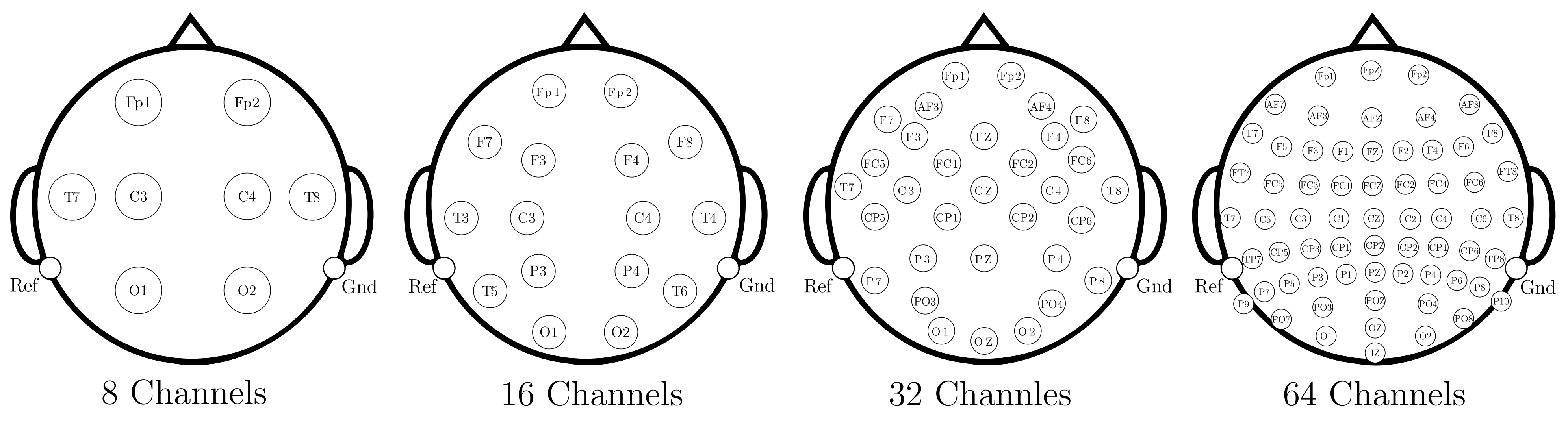
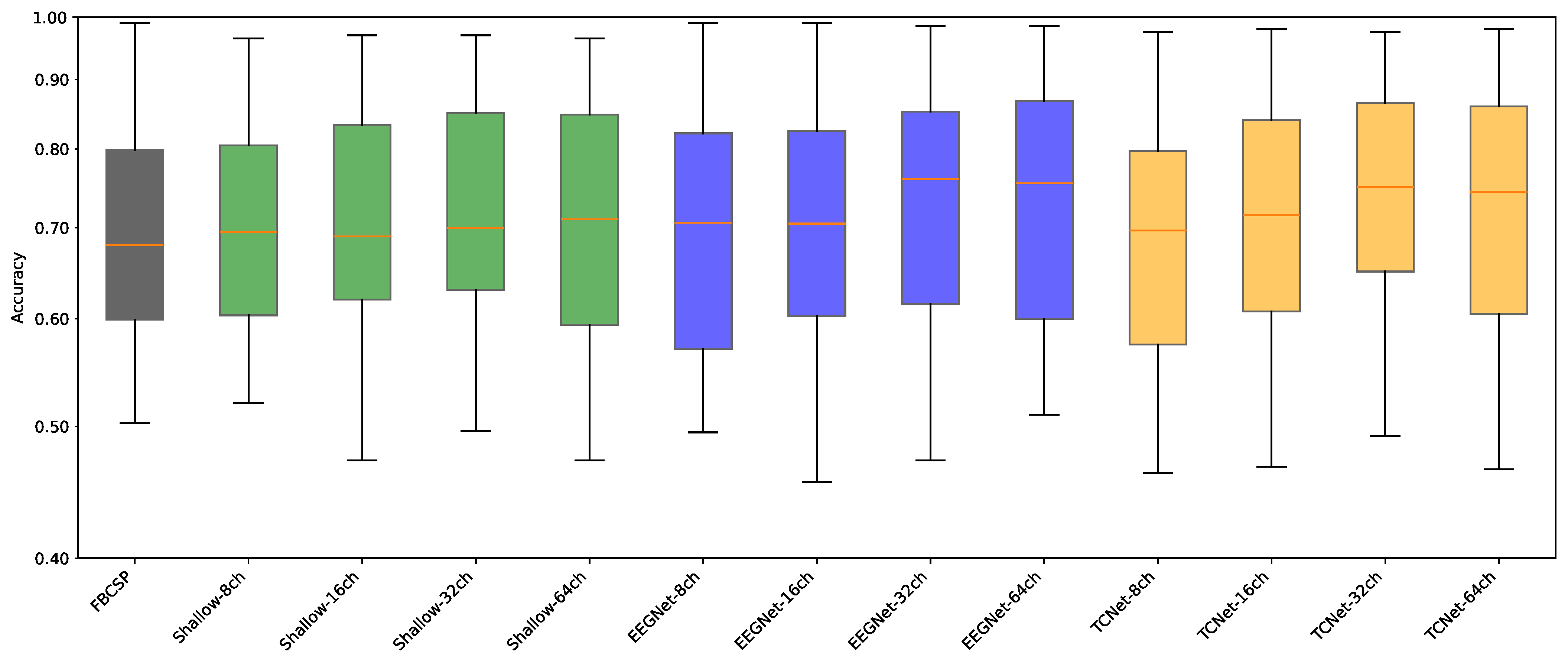
• Comprehensive evaluation across multiple architectures and conditions: We conduct a rigorous evaluation of our framework on a 52-subject dataset, testing its efficacy across three distinct deep learning architectures (ShallowConvNet, EEGNet, TCNet Fusion) and under varying channel montage densities (8, 16, 32, and 64 channels).
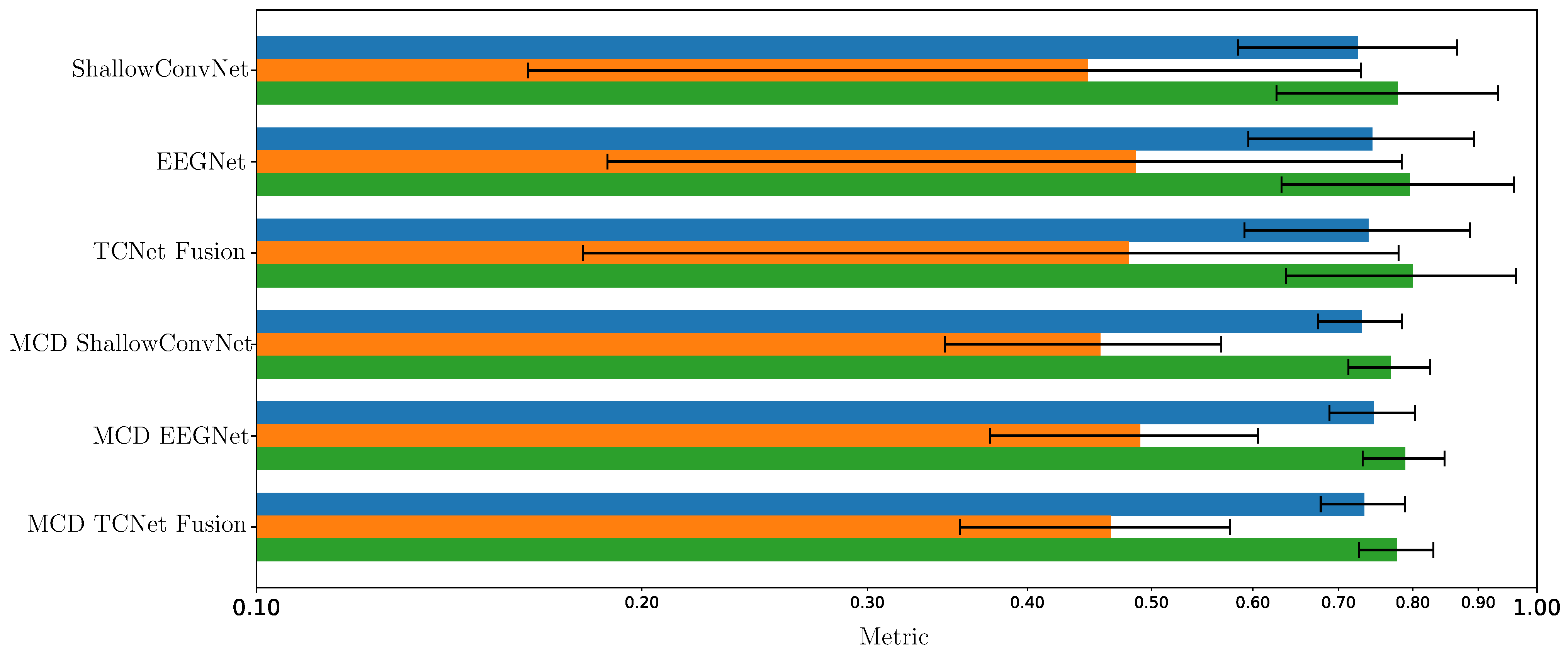
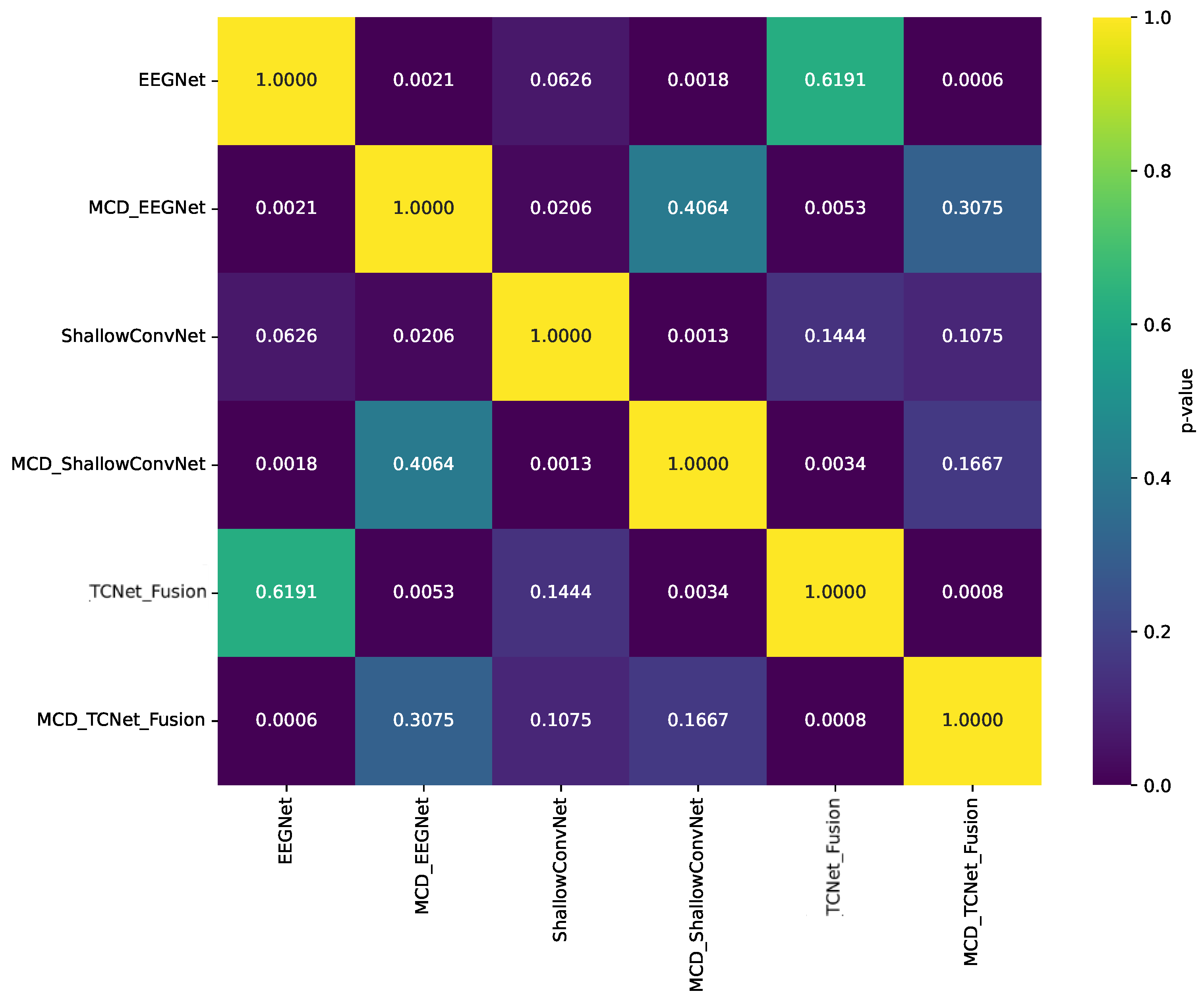
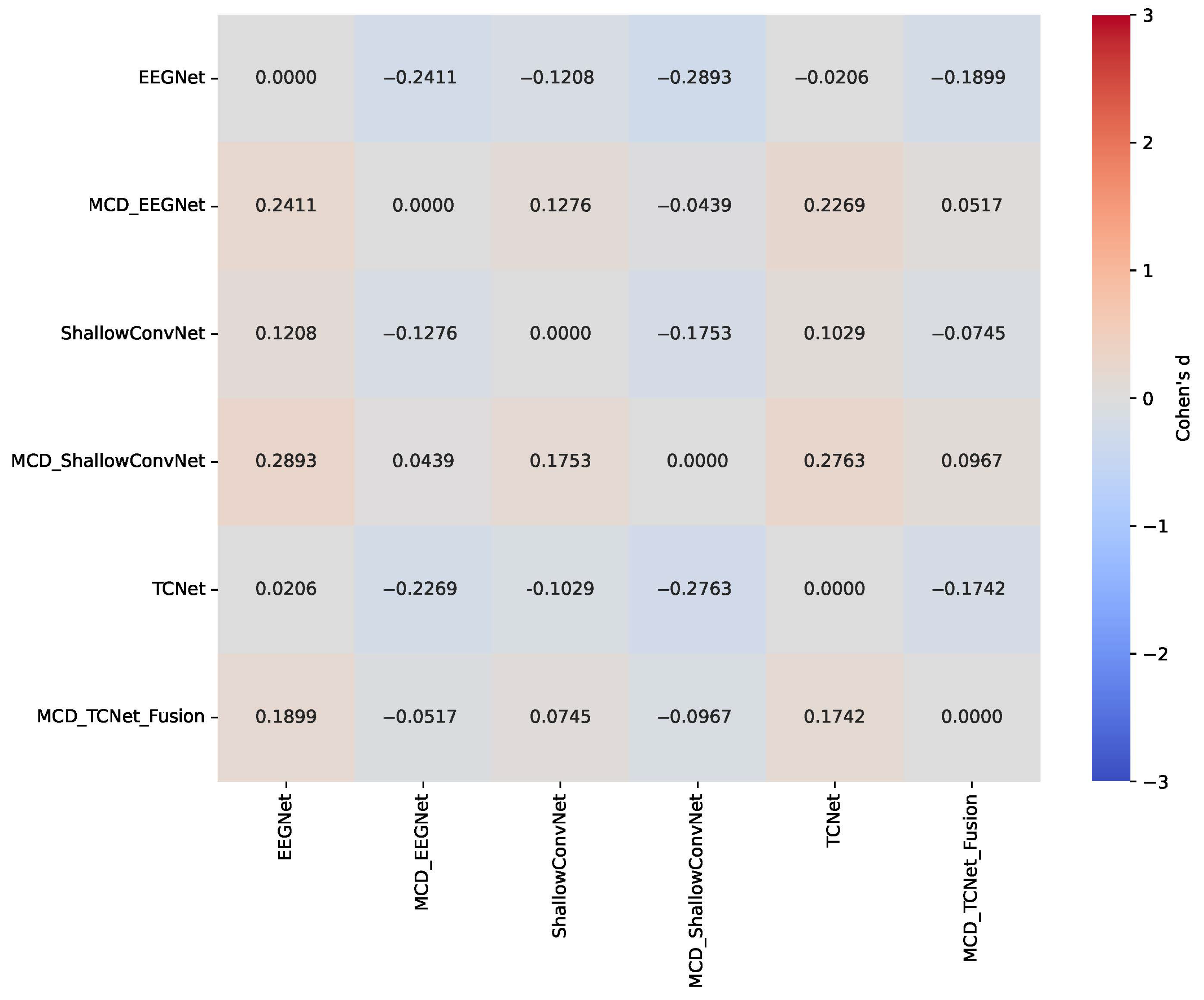
• Statistically validated performance improvement: We provide statistically significant evidence (p < 0.05) that our MCD-enhanced models consistently outperform their baseline counterparts, with particularly notable gains for low-performing subjects, thereby enhancing both accuracy and inter-subject consistency.
• Enhanced interpretability through CAMs: We demonstrate through LayerCAM visualizations that our uncertainty-aware approach transforms diffuse, difficult-to-interpret spatial attention maps into focused, neurophysiologically plausible topograms, significantly improving model transparency and clinical trust.

The remainder of this paper is organized as follows: Section 2 reviews related work in the field of EEG-based BCI systems. Section 3 details the methods, including baseline feature extraction with FBCSP and the implementation of three DL models (ShallowConvNet, EEGNet, and TCNet Fusion) tailored to EEG signal characteristics, alongside channel dropout and CAM integration. Section 4 outlines the experimental setup, covering the MI-EEG dataset, preprocessing, montage reduction, and evaluation metrics for robustness and interpretability across subject groups. Section 5 presents results and discussion, analyzing classification accuracy, dropout effects on stability, and LayerCAM-based spatiotemporal patterns. Finally, Section 6 concludes with key findings and future directions for uncertainty-aware MI classification.

2. Related Work

2.1. Deep Learning for MI-EEG Classification

The adoption of DL has marked a significant paradigm shift in MI-EEG classification, moving the field beyond traditional machine learning pipelines that rely on handcrafted features [35]. As systematically reviewed by Saibene et al. [36], this transition has been driven by the increasing availability of large public datasets and the inherent ability of DL models to learn relevant hierarchical features directly from raw or minimally processed EEG data. Convolutional neural networks (CNNs) have been the dominant architecture in this domain. Foundational models like ShallowConvNet [37] and the more compact EEGNet [38] were specifically designed to capture the unique spatiotemporal characteristics of EEG signals and have become standard benchmarks in the field. These models and their variants are the most frequently used architectures in recent literature, demonstrating robust performance across various MI paradigms [36]. Subsequent innovations have focused on enhancing temporal modeling capabilities. For instance, TCNet Fusion [39] integrated Temporal Convolutional Networks (TCNs) to better handle long-range dependencies, while other hybrid models have combined CNNs with recurrent neural networks (RNNs) like LSTMs to process EEG as sequential data [40,41]. More recently, the field has begun to explore architectures inspired by advances from other domains. Graph convolutional networks (GCNs) have been employed to explicitly model the spatial relationships between EEG electrodes based on their physical proximity, aiming to learn more neurophysiologically plausible spatial filters [42]. The most current trend, as highlighted by multiple recent studies, is the adaptation of Transformer models for EEG analysis. Architectures like CNet [43] and others [44,45] leverage self-attention mechanisms to capture global dependencies across both time and space, showing great promise for improving decoding accuracy. Despite this rapid architectural innovation, Saibene et al. [36] note that consistent challenges related to overfitting, reproducibility, and interpretability remain central concerns. Our work, therefore, does not aim to propose a new backbone architecture, but rather to enhance the most established and widely used CNN-based frameworks by introducing a unified solution for robustness and interpretability, two of the most critical hurdles for the clinical translation of these powerful models.

2.2. Sparse Electrode Configurations

For BCI systems to transition from laboratory environments to practical, everyday use, they must be portable, non-intrusive, and easy to set up. This has driven a significant research effort toward developing systems that function effectively with sparse electrode configurations, i.e., using a minimal number of EEG channels [36,46]. While traditional, high-density EEG caps provide excellent spatial resolution, their long preparation times, need for conductive gel, and user discomfort make them unsuitable for many real-world applications, particularly for stroke patients or home-use scenarios [47]. However, reducing the number of channels introduces a fundamental trade-off between portability and performance. As noted by Shiam et al. [48], using fewer channels can lead to the loss of critical information and an increase in susceptibility to noise and artifacts, often resulting in degraded classification accuracy. A primary challenge, therefore, lies in intelligently selecting the most informative subset of channels. A large body of work has focused on this, using various criteria for channel ranking and selection. For instance, Shiam et al. [48] propose a novel entropy-based method to identify channels with the highest information content, demonstrating that a carefully selected subset can outperform a full-channel configuration. Other approaches have utilized correlation-based metrics [49] or advanced algorithms like the binary gravitational search algorithm (BGSA) to optimize channel placement [50]. More recently, research has shifted towards developing wearable, few-channel devices that are inherently designed for practicality. Rao et al. [47] introduced a wearable headband with just four wet electrodes, specifically targeting the motor and occipital cortices. Their work demonstrates that such a sparse system can achieve high online classification accuracy (over 76%), comparable to a mature commercial wired system, while drastically reducing setup time. This highlights the feasibility of creating effective, low-channel count BCIs for rehabilitation. Despite these successes, the challenge of inter-subject variability remains; the optimal sparse configuration for one user may not be ideal for another [51]. Our work directly engages with this problem by using channel dropout not only as a regularization technique but also as a way to simulate the structural variability inherent in sparse-channel BCI systems, thereby building models that are more robust to these practical constraints.

2.3. Explainable AI in EEG-Based BCI Systems

As deep learning models increase in complexity, their “black-box” nature becomes a significant barrier to clinical trust and user adoption, especially in high-stakes BCI applications [52]. The field of explainable AI (XAI) has emerged to address this challenge by developing methods to render model decisions transparent and understandable. As systematically reviewed by Rajpura et al. [53], the primary motivations for applying XAI in BCI are to justify model predictions, debug and improve model performance, and discover new neurophysiological insights. XAI techniques for EEG can be broadly categorized. One major group includes model-agnostic, perturbation-based methods like LIME and SHAP, which assess feature importance by observing how predictions change when inputs are altered [54]. Another prominent category, particularly suited for the CNNs commonly used in EEG decoding, consists of gradient-based methods. These techniques, such as Saliency Maps [55], Grad-CAM [56], and its variants like LayerCAM [29], produce “relevance heatmaps”. In the context of BCI, these heatmaps are often visualized as topoplots that highlight which EEG channels and time-frequency components were most influential for a given classification. Such visualizations are crucial for validating that a model is learning neurophysiologically plausible patterns (e.g., activity over the sensorimotor cortex) rather than relying on spurious artifacts [57]. The review by Rajpura et al. [53] further emphasizes that effective XAI must consider the entire “design space”, including not just the how (the technique) but also the what (the application, e.g., motor imagery), the who (the stakeholder, e.g., a clinician vs. a developer), and the why (the purpose, e.g., justification vs. discovery). Our work aligns with this holistic view by adopting LayerCAM as our visualization tool, chosen for its ability to produce high-resolution, class-discriminative explanations that can be directly mapped back to the sensor space, thereby providing a clear and interpretable window into the model’s decision-making process.

2.4. Uncertainty Estimation in Neural Models

Standard DL models, while excelling at function approximation, typically produce point estimates and lack an intrinsic mechanism to express prediction confidence. This absence of uncertainty modeling, particularly epistemic uncertainty (i.e., uncertainty in the model’s parameters due to limited data), can lead to overconfident predictions, a critical limitation in safety-conscious applications like brain–computer interfaces (BCI), where incorrect decisions may have significant consequences [58]. To address this, the field of Bayesian deep learning has increasingly focused on modeling uncertainty by learning a probability distribution over model weights, rather than relying on a single point estimate. While full Bayesian inference provides a robust framework for uncertainty quantification, which aims to reliably measure a model’s confidence in its predictions, it is often computationally intractable for large models. As detailed by Hu et al. [59], various approximation methods have been developed to overcome these challenges, such as variational inference, Laplace approximation, and sampling-based methods. Among these, Monte Carlo dropout (MCD) [60] has emerged as a particularly popular and computationally efficient technique. MCD utilizes dropout during inference to generate an ensemble of predictions from a single model, where the variance of these predictions serves as an estimate of epistemic uncertainty. Alternatively, non-Bayesian approaches, such as deep ensembles, have been developed. In these approaches, multiple independently trained models are combined, and their predictive disagreement is used to quantify uncertainty [61]. This method has gained popularity, especially in scenarios where full Bayesian inference is computationally prohibitive. A key advantage of deep ensembles is their ability to explore diverse model architectures and weight initializations, which provides reliable uncertainty estimates. For example, Tveter et al. [62] demonstrated that deep ensembles significantly improve prediction performance and uncertainty estimation in EEG analysis. By performing multiple forward passes on the same input, deep ensembles generate a distribution of predictions, with the variance acting as a proxy for epistemic uncertainty. This strategy has been successfully applied in EEG-based classification tasks, such as epileptic seizure detection, where it helps to reject the most uncertain data points, thereby improving system reliability. Building on these principles, our work leverages the computational efficiency of MCD, which has been shown to enhance both accuracy and the reliability of uncertainty estimates [59].

The four research areas, i.e., accuracy, robustness, transparency, and portability, have evolved separately, with each focusing on improving one aspect of BCI systems. However, a significant gap remains: no unified framework addresses these challenges simultaneously. A robust yet uninterpretable model lacks clinical trust, while an interpretable but unreliable model is ineffective. This study proposes a solution by integrating MCD for uncertainty-aware robustness with LayerCAM for fine-grained interpretability, creating a synergistic pipeline. This combination not only enhances performance but also ensures that the improvements are grounded in focused and neurophysiologically plausible brain patterns.

3. Materials and Methods

3.1. Baseline Feature Extraction of Spatiotemporal Characteristics

Given a dataset composed by ${\{X_n\in {\mathbb{R}}^{C\times T}\}}_{n=1}^N$, consisting of $N\in \mathbb{N}$ EEG trials—where C denotes the number of channels and T the number of temporal samples per trial—the classification task aims to learn a function $f:{\mathbb{R}}^{C\times T}\to {\mathbb{R}}^K$ that predicts the binary label $y_n\in \{0,1\}$ ($K=2$), corresponding to the brain’s neural responses to left- and right-hand MI, respectively.

As a classical baseline, we include the Filter Bank Common Spatial Pattern (FBCSP) method, widely used in MI-BCI systems for its effectiveness in extracting subject-specific spatio-spectral features. The baseline MI binary classification approach involves spatial filtering via linear transformations of the EEG data to enhance class separability—specifically, by maximizing the variance of signals associated with one class while minimizing it for the other [63,64]. The EEG signals are first passed through a filter bank comprising bandpass filters, typically centered on canonical sub-bands $b_i$ (e.g., mu, alpha, beta) or custom frequency ranges. This process yields filtered EEG segments $X_{b_i}\in {\mathbb{R}}^{C\times T}$. Following the FBCSP procedure [65], features are extracted by computing the log-variance of the spatially filtered signals ${\overline{X}}_{b_i}$, as given by the following:

$$v_{b_i}=\log \left({\displaystyle \frac{\mathrm{diag}\left({\overline{X}}_{b_i}{\overline{X}}_{b_i}^{\top }\right)}{\mathrm{tr}\left({\overline{X}}_{b_i}{\overline{X}}_{b_i}^{\top }\right)}}\right),$$

where $\mathrm{diag}(·)$ extracts the diagonal elements of the covariance matrix, $\mathrm{tr}(·)$ denotes the trace operator, and ${\overline{X}}_{b_i}={\overline{W}}_{b_i}^{\top }{X}_{b_i}$ represents the spatially filtered signal using projection matrix ${\overline{W}}_{b_i}$, which contains the most discriminative spatial filters for sub-band $b_i$.

3.2. Deep Learning Frameworks for Feature Extraction of MI Responses

Building upon the baseline FBCSP approach, we consider three well-established DL architectures, each specifically designed to address the unique spatiotemporal characteristics of EEG signals in MI classification. These models have demonstrated competitive performance and complementary strengths in recent EEG-based BCI benchmarks [36], providing a comprehensive foundation for evaluating the effectiveness of our proposed channel dropout and CAM integration approach.

∗

ShallowConvNet Framework. This model learns a hierarchical mapping through stacked layers ${\varphi }_3\circ {\varphi }_2\circ {\varphi }_1$, as follows [37,65]:

$$\begin{array}{ccc}\hfill \mathrm{Temporal}\mathrm{Conv}:{\varphi }_1:Z_{f,c,t}& =\sum _{k=0}^{K_t-1}{W}_{f,k,c}{X}_{c,t+k}+b_f,\hfill & Z\in {\mathbb{R}}^{F_t\times C\times (T-K_t+1)}\hfill \\ \hfill \mathrm{Spatial}\mathrm{Conv}:{\varphi }_2:Y_{f,s,t}& =\sum _{c=1}^C{V}_{f,s,c}{Z}_{f,c,t}+b_{f,s},\hfill & Y\in {\mathbb{R}}^{F_t\times F_s\times (T-K_t+1)}\hfill \\ \hfill \mathrm{Nonlinear}\mathrm{Pooling}:{\varphi }_3:P_{f,s,m}& ={\displaystyle \frac{1}{P}}\sum _{t=(m-1)S+1}^{(m-1)S+P}{\left(Y_{f,s,t}\right)}^2,\hfill & P\in {\mathbb{R}}^{F_t\times F_s\times M}\hfill \end{array}$$

where $K_t=25$, $F_s$ is the number of spatial filters, and $M=⌊{\displaystyle \frac{T-K_t+1-P}{S}}+1⌋$.

∗

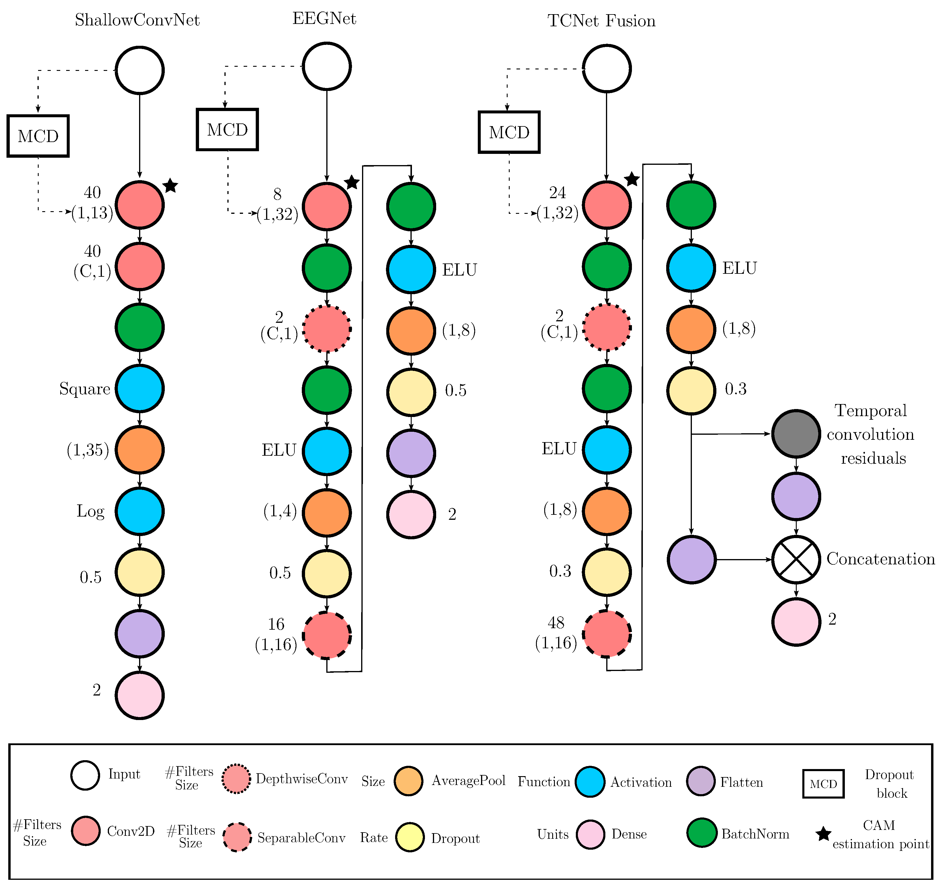
EEGNet Framework. In this architecture, feature extraction is carried out through a sequence of convolutional blocks ${\psi }_3\circ {\psi }_2\circ {\psi }_1$, structured as [38]:

$$\begin{array}{ccc}\hfill \mathrm{Temporal}\mathrm{Conv}:{\psi }_1:Z_{f,c,t}^{EEG}& =\sum _{k=0}^{K_t^{EEG}-1}{W}_{f,k,c}^{EEG}{X}_{c,t+k}+b_f^{EEG},\hfill & Z^{EEG}\in {\mathbb{R}}^{F_1\times C\times (T-K_t^{EEG}+1)}\hfill \\ \hfill \mathrm{Depthwise}\mathrm{Conv}:{\psi }_2:D_{i,s,t}& =\sum _{k=0}^{K_d-1}{U}_{i,k,s}{Z}_{i,s,t+k}^{EEG}+b_i,\hfill & D\in {\mathbb{R}}^{F_1\times F_s\times (T-K_t^{EEG}-K_d+2)}\hfill \\ \hfill \mathrm{Separable}\mathrm{Conv}:{\psi }_3:S_{j,t}& =\sum _{i=1}^{F_1}\sum _{s=1}^{F_s}{Q}_{j,i,s}{D}_{i,s,t}+b_j,\hfill & S\in {\mathbb{R}}^{F_2\times (T-K_t^{EEG}-K_d+2)}\hfill \end{array}$$

where $F_1$ and $F_2$ denote the number of temporal and separable filters, respectively; $K_t^{EEG}$ and $K_d$ are the kernel sizes for the temporal and depthwise convolutions; and $F_s$ is the number of spatial filters. Each block is followed by batch normalization and non-linear activation.

∗

TCNet (Temporal Convolutional Network) Framework. TCNet extends the prior architectures by integrating temporal convolutional modules with residual connections [66,67]. The model combines filter bank design with deep temporal processing through the sequential application of blocks ${\xi }_5\circ {\xi }_4\circ {\xi }_3\circ {\xi }_2\circ {\xi }_1$, as follows:

$$\begin{array}{ccc}\hfill \mathrm{Initial}\mathrm{Temporal}\mathrm{Conv}:{\xi }_1:T_{f,c,t}& =\sum _{k=0}^{K_i-1}{G}_{f,k,c}{X}_{c,t+k}+b_f^T,\hfill & T\in {\mathbb{R}}^{F_0\times C\times (T-K_i+1)}\hfill \\ \hfill \mathrm{Filter}\mathrm{Bank}\mathrm{Conv}:{\xi }_2:B_{f,c,t}& =\sum _{k=0}^{K_f-1}{H}_{f,k,c}{T}_{f,c,t+k}+b_f^B,\hfill & B\in {\mathbb{R}}^{F_0\times C\times (T-K_i-K_f+2)}\hfill \\ \hfill \mathrm{Spatial}\mathrm{Conv}:{\xi }_3:C_{f,s,t}& =\sum _{c=1}^C{J}_{f,s,c}{B}_{f,c,t}+b_{f,s}^C,\hfill & C\in {\mathbb{R}}^{F_0\times F_s\times (T-K_i-K_f+2)}\hfill \\ \hfill \mathrm{Residual}\mathrm{Temporal}\mathrm{Block}:{\xi }_4:R_{f,s,t}^{\left(l\right)}& =C_{f,s,t}+{\Gamma }^{\left(l\right)}\left(C_{f,s,t}\right),\hfill & \mathrm{for}l=1,2,\dots ,L\hfill \\ \hfill \mathrm{Global}\mathrm{Avg}\mathrm{Pooling}:{\xi }_5:A_f& ={\displaystyle \frac{1}{T^{\prime }}}\sum _{t=1}^{T^{\prime }}{R}_{f,s,t}^{\left(L\right)},\hfill & A\in {\mathbb{R}}^{F_0\times F_s}\hfill \end{array}$$

where $K_i$ and $K_f$ are the kernel sizes for the initial and filter bank convolutions, $F_0$ is the number of feature maps, L is the number of residual blocks, $T^{\prime }=T-K_i-K_f+2$, and ${\Gamma }^{\left(l\right)}$ denotes a temporal convolutional block with dilated convolutions. The dilation factor increases with l, enabling exponential growth in the receptive field while preserving temporal resolution.

The final classification stage in all three DL frameworks is performed by a fully connected layer applied to the flattened output of the last feature extraction layer $\widehat{P}$, with the classification computed as

$${\widehat{y}}_c=\mathrm{softmax}\left(\sum _i{\hat{W}}_{c,i}^{\mathrm{fc}}{\widehat{P}}_i+{\widehat{b}}_c^{\mathrm{fc}}\right),$$

where $\widehat{y}\in {\mathbb{R}}^K$ denotes the class probability distribution over K classes. In this expression, $\widehat{P}\in {\mathbb{R}}^d$ is the d-dimensional feature vector obtained by applying global average pooling to the final convolutional feature maps. The matrix ${\widehat{W}}^{\mathrm{fc}}\in {\mathbb{R}}^{K\times d}$ contains the weights of the fully connected layer, and ${\widehat{b}}^{\mathrm{fc}}\in {\mathbb{R}}^K$ represents the corresponding bias vector.

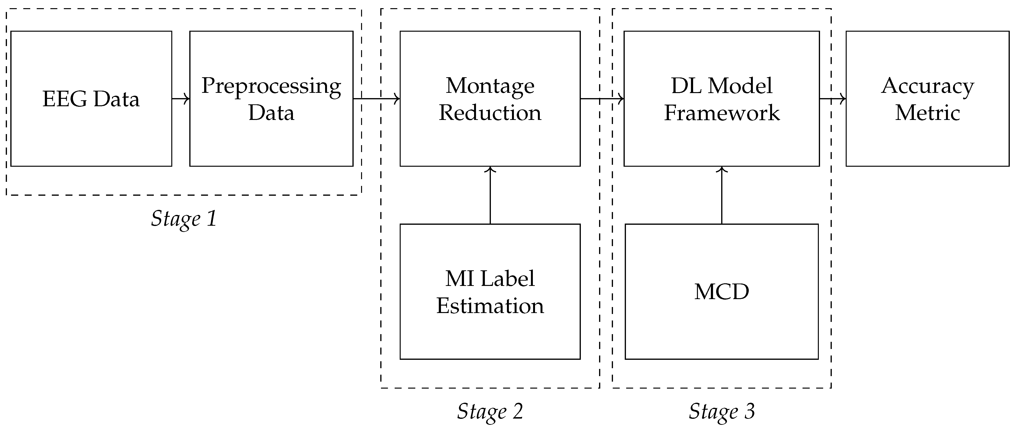
3.3. Monte Carlo Dropout with CAM Integration for MI Classification

To address the limitations of traditional approaches and enhance both robustness and interpretability in EEG-based MI classification, we integrate Monte Carlo dropout (MCD) with class activation maps (CAMs) across the deep learning architectures described above [68]. This integration provides a unified framework that simultaneously quantifies prediction uncertainty and visualizes spatiotemporal patterns critical for MI classification. It is important to note their distinct roles: MCD is a model component whose contribution is evaluated via an ablation study (comparing models with and without it), whereas CAMs is a post-hoc visualization technique used to interpret the model’s behavior, not to alter its performance.

Channel dropout is applied by introducing a dropout mask ${\mathit{ϵ}}^{\left(i\right)}\sim \mathrm{Bernoulli}(1-p)$ component-wise to the input EEG tensor $\mathbf{X}\in {\mathbb{R}}^{C\times T}$, such that the modified input becomes ${\mathbf{X}}^{\left(i\right)}=\mathbf{X}\odot {\mathit{ϵ}}^{\left(i\right)}$, where ⊙ denotes element-wise multiplication. For a given layer output $\mathbf{h}\in {\mathbb{R}}^d$, the MCD operation is defined as follows:

$$\begin{array}{cc}\hfill \mathrm{MCD}\mathrm{Operation}:{\mathbf{h}}^{\left(i\right)}& =\mathbf{h}\odot {\mathit{ϵ}}^{\left(i\right)},\mathrm{Scaled}\mathrm{Output}:{\tilde{\mathbf{h}}}^{\left(i\right)}={\displaystyle \frac{{\mathbf{h}}^{\left(i\right)}}{1-p}},{\tilde{\mathbf{h}}}^{\left(i\right)}\in {\mathbb{R}}^d,\hfill \end{array}$$

where $p\in [0,1]$ is the dropout probability, ${\mathit{ϵ}}^{\left(i\right)}\in {\{0,1\}}^d$ is a random mask vector sampled from a Bernoulli distribution with success probability $1-p$. The scaling factor ${\displaystyle \frac{1}{1-p}}$ preserves the expected activation magnitude, ensuring $\mathbb{E}\left[{\tilde{h}}_j^{\left(i\right)}\right]=h_j$.

The integration of MCD goes beyond uncertainty quantification, serving as a performance-enhancing technique grounded in established machine learning principles. Its effectiveness can be explained through two theoretical lenses: (1) as a regularizer, channel dropout mitigates overfitting by randomly deactivating EEG channels during training, encouraging the model to learn more robust and generalizable representations of motor imagery; and (2) as an approximate Bayesian ensemble, multiple forward passes with different dropout masks during inference approximate the behavior of an ensemble of neural networks [60], reducing prediction variance and enhancing stability [69]. These combined effects underpin the observed performance gains in our framework.

During inference, MCD generates T stochastic predictions, which are then augmented by CAMs to visualize spatially relevant features. This integration is formalized as [70]:

$$\begin{array}{cc}\hfill \mathrm{Stochastic}\mathrm{Predictions}:{\widehat{\mathbf{y}}}^{\left(i\right)}& =f_{\theta }(\mathbf{X};{\mathit{ϵ}}^{\left(i\right)}),i=1,2,\dots ,T,\hfill \\ \hfill \mathrm{Predictive}\mathrm{Mean}:\overline{\mathbf{y}}& ={\displaystyle \frac{1}{T}}\sum _{i=1}^T{\widehat{\mathbf{y}}}^{\left(i\right)},\hfill \\ \hfill \mathrm{Predictive}\mathrm{Variance}:{\sigma }^2& ={\displaystyle \frac{1}{T}}\sum _{i=1}^T{\parallel {\widehat{\mathbf{y}}}^{\left(i\right)}-\overline{\mathbf{y}}\parallel }^2,\hfill \\ \hfill \mathit{CAM}\mathit{Computation}:M_c\left(\mathbf{X}\right)& =\sum _k{w}_k^c·A_k\left(\mathbf{X}\right),w_k^c={\displaystyle \frac{1}{Z}}\sum _{i=1}^T{\displaystyle \frac{\partial {\widehat{y}}_c^{\left(i\right)}}{\partial A_k\left(\mathbf{X}\right)}},\hfill \end{array}$$

(1)

where $f_{\theta }(·;{\mathit{ϵ}}^{\left(i\right)})$ is the network with dropout mask ${\mathit{ϵ}}^{\left(i\right)}$, ${\widehat{\mathbf{y}}}^{\left(i\right)}\in {\mathbb{R}}^K$ is the prediction vector, $\overline{\mathbf{y}}$ is the final output, and ${\sigma }^2$ quantifies uncertainty. For CAM computation, $M_c\left(\mathbf{X}\right)$ is the activation map for class c, $A_k\left(\mathbf{X}\right)$ is the activation of unit k in the target layer, and $w_k^c$ is the importance weight averaged over T MCD samples, normalized by Z (number of spatial locations), with gradients ${\displaystyle \frac{\partial {\widehat{y}}_c^{\left(i\right)}}{\partial A_k\left(\mathbf{X}\right)}}$ reflecting feature relevance.

4. Experimental Set-Up

4.1. Evaluating Framework

This study proposes a channel-wise dropout-based framework augmented with CAMs to enhance the interpretability of neural network decisions. The framework dynamically identifies spatial (channel-level) contributions that vary temporally and may contribute to misclassifications in MI-evoked brain responses.

As shown in Figure 1, the framework comprises the following stages:

∗

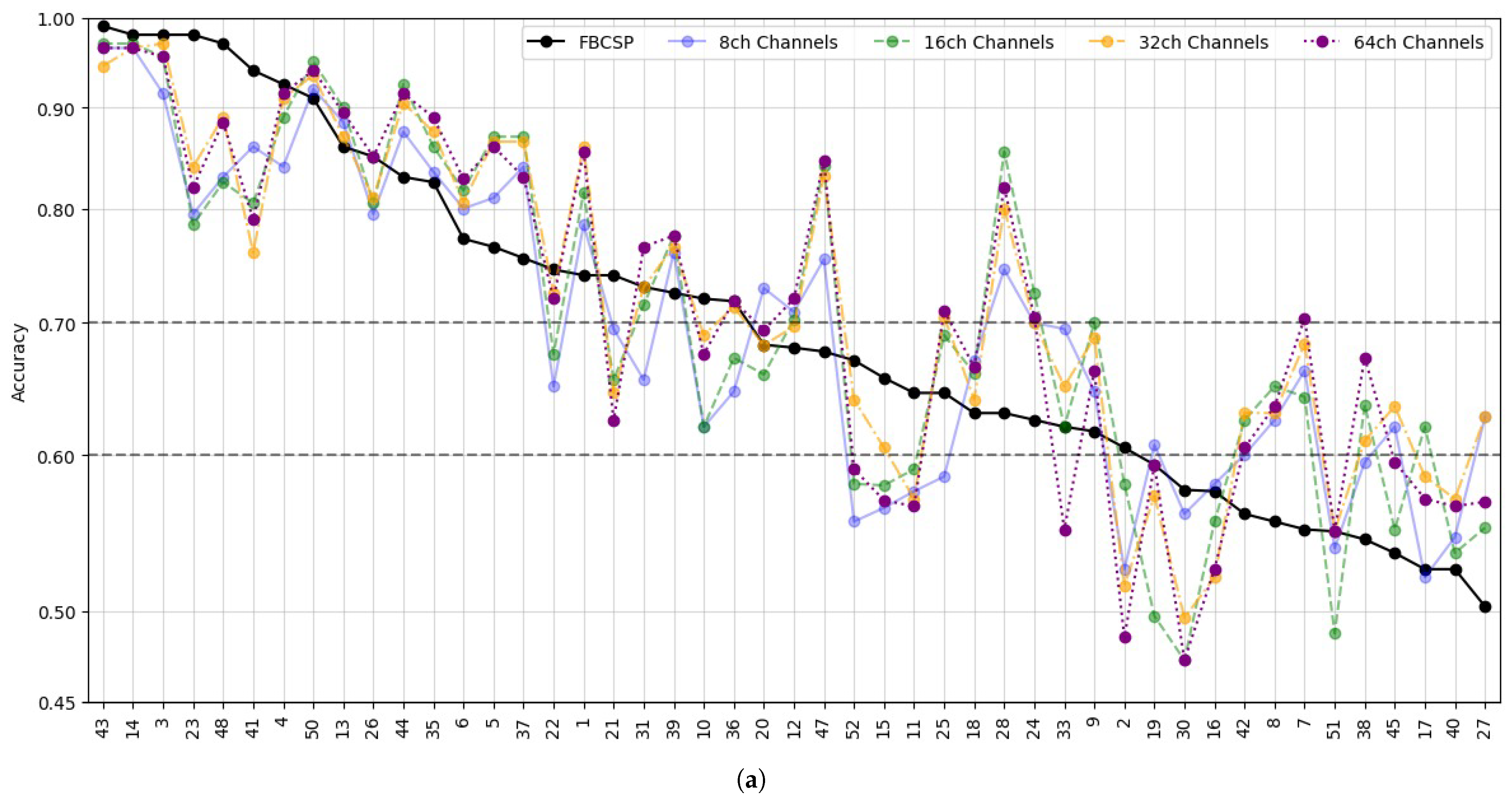
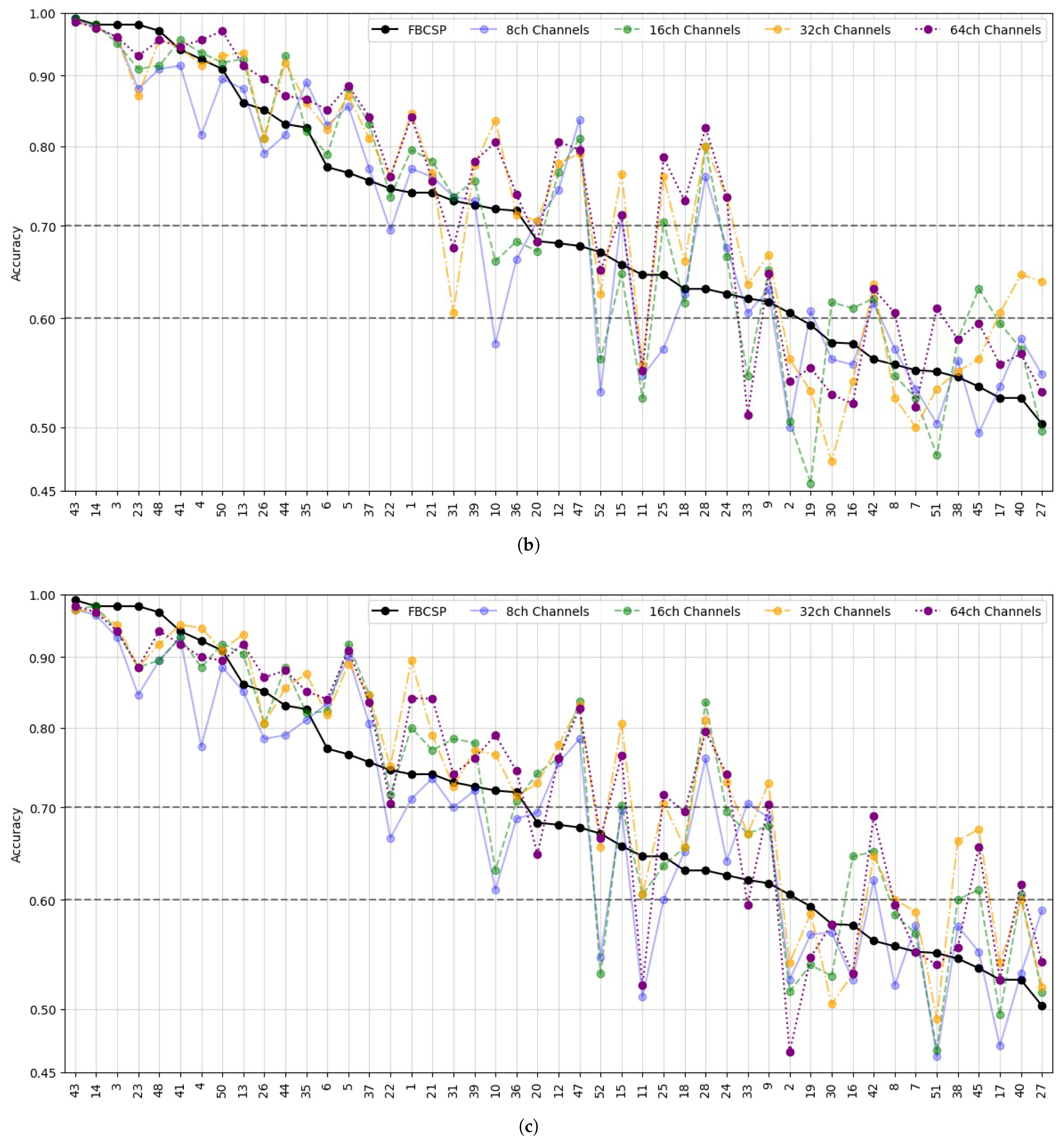
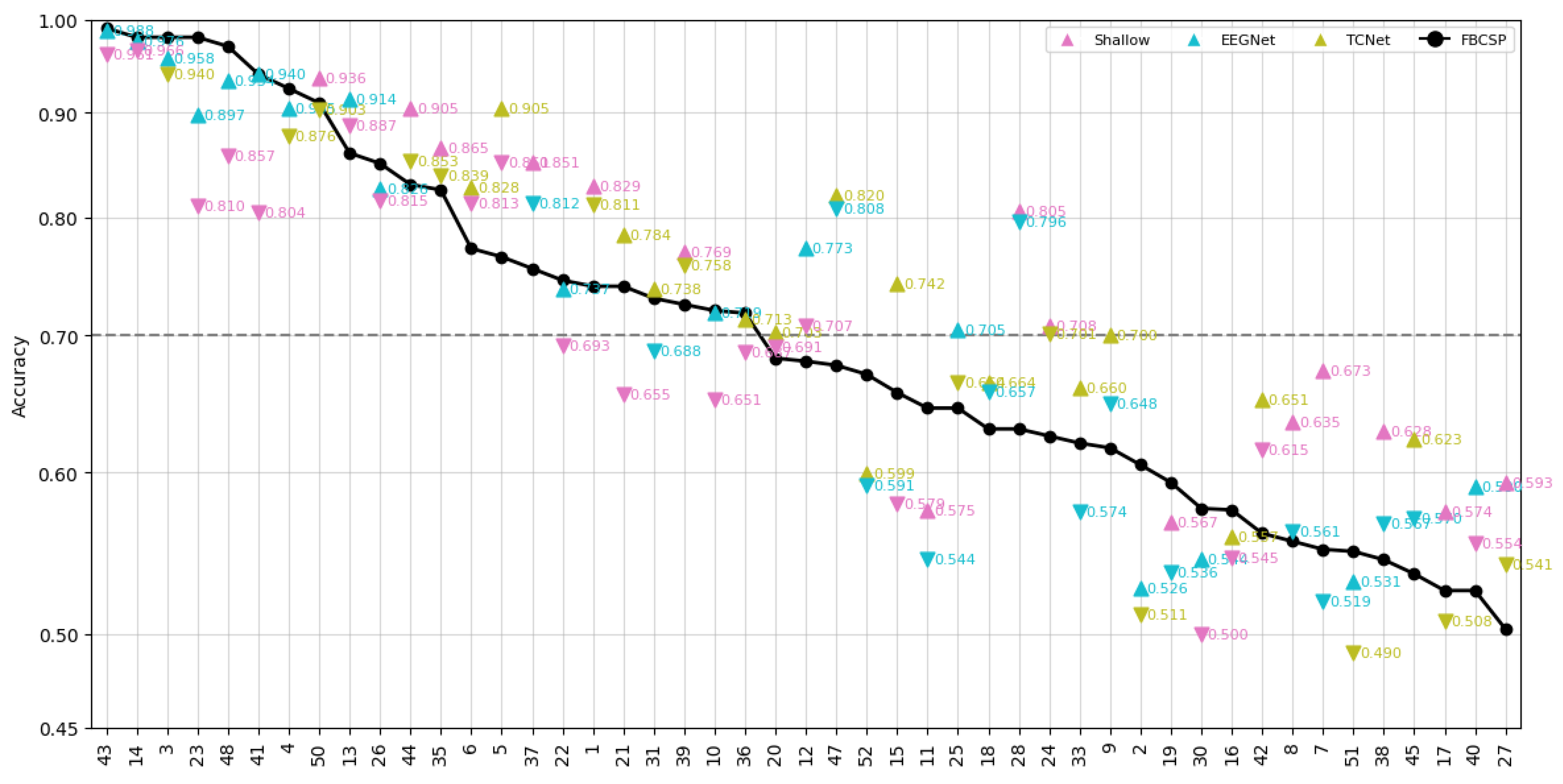
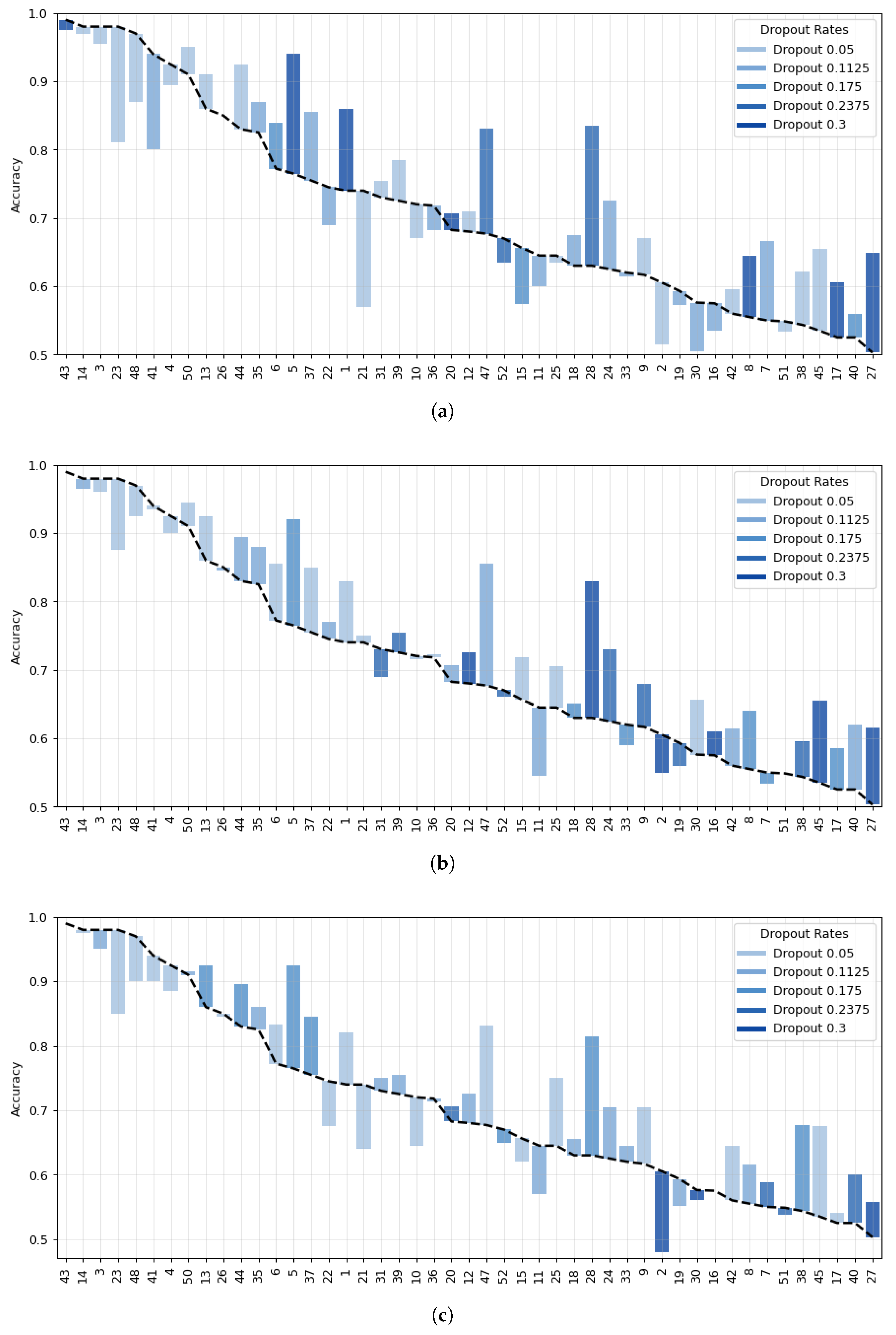
Data Preprocessing and Montage Reduction. We evaluate the impact of EEG montage size on model generalizability, hypothesizing that excessive channels promote overfitting on spatially correlated artifacts rather than task-specific MI neural dynamics. Montage sizes $N_c\in \{8,16,32,64\}$ are tested separately for the best- and worst-performing subjects. Subjects are stratified into high (best)- and low (worst)-performance cohorts based on evaluated trial accuracy (<70% or ≥70%). This serves as a conventional reference for evaluating the benefits of DL-based frameworks in ranking subjects based on their trial-level classification accuracy.

∗

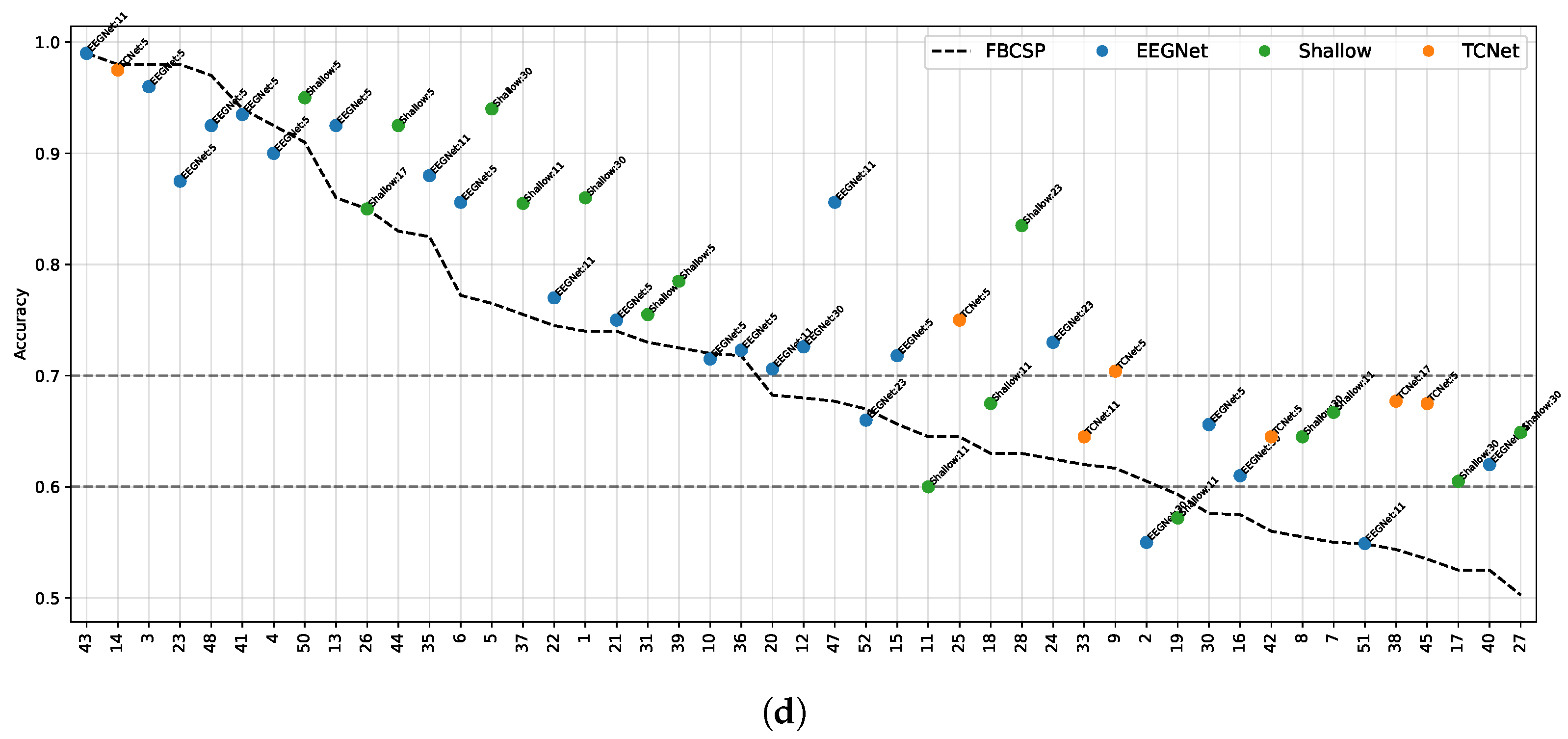
Subject Grouping Based on the Classification Accuracy of MI Responses. We evaluate three Neural network models for EEG-based classification, EEGNet and ShallowConvNet, for their real-time applicability, alongside the advanced TCNet Fusion architecture for enhanced performance. As stated above, we use FBCSP as a classical baseline for extracting subject-specific spatio-spectral features. This provides a conventional reference to assess the benefits of deep learning-based approaches.

∗

Spatio-temporal uncertainty estimation. MCD is applied to assess each model’s ability to learn robust, channel-independent features, thereby reducing overfitting and improving generalization. Furthermore, MCD is combined with CAMs to estimate spatiotemporal uncertainty and enhance model interpretability. Specifically, the variance computed across CAMs is overlaid onto the original CAM representation, highlighting regions where the model exhibits reduced certainty in its interpretation of MI responses.

4.2. Motor Imagery EEG Data Collection

For validation purposes, we utilize an electroencephalogram dataset from MI-based brain–computer interface experiments [71], comprising data from 52 healthy participants (mean age: 24.8 ± 3.86 years) (available online: http://gigadb.org/dataset/100295, accessed on 1 December 2024). Of note, subjects labeled 29, 32, 34, 46, and 49 were excluded because their data lacked sufficient discriminative power, a practice also followed in [32].

The experimental protocol requires participants to imagine left- and right-hand movements in response to standardized visual cues displayed on a screen. EEG signals are recorded using a 64-channel Biosemi ActiveTwo system at a sampling rate of 512 Hz. Additionally, simultaneous electromyographic recordings are conducted to ensure the absence of actual hand movements during MI trials. The experimental paradigm, illustrated in Figure 2, follows a structured MI task designed to elicit EEG data corresponding to imagined left- and right-hand movements. Participants are seated comfortably with armrests and positioned facing a monitor on which visual cues are displayed. Each trial begins with a black screen and a fixation cross for 2 s to allow for task preparation. This is followed by a visual instruction—either “Left hand” or “Right hand”—presented for 3 s, prompting participants to imagine sequential finger movements corresponding to the indicated hand. Afterward, a blank screen is displayed for a randomized interval of 4.1 to 4.8 s, serving as a rest period and reducing task predictability. Note that the protocol emphasizes kinesthetic experience of movement (i.e., the sensation of muscle activation), rather than visual imagery.

All participants completed five to six runs per session, with each run consisting of 100–120 trials per MI class. Each trial is carefully structured to ensure consistency in data collection, as participants follow standardized visual cues to perform the MI task. Trials are evenly distributed between left- and right-hand imagery conditions, yielding a balanced dataset for analysis.

Additionally, feedback is provided after each run to enhance participant engagement. This dataset enables robust validation through event-related desynchronization/synchronization analysis, classification accuracy metrics, and identification of noisy or artifact-contaminated trials. The comprehensive experimental design serves as a valuable resource for studying performance variability in MI-BCI systems and for developing subject-independent models.

4.3. EEG Preprocessing and Reduction of EEG-Channel Montage Set-Up

The collected EEG signals are preprocessed prior to training to ensure high data quality. First, an average reference is applied and then re-referenced to include the original reference electrode, thereby preserving the full rank of the data [72]. A fifth-order Butterworth bandpass filter (4–40 Hz) is subsequently applied to isolate the relevant frequency range, as suggested in [73]. Since the dataset focuses on motor imagery rather than higher-order cognitive processes such as multisensory integration, the analysis targets three primary frequency bands: Theta (4–8 Hz), Alpha (8–13 Hz), and Beta (13–32 Hz) [74]. The Gamma band (above 40 Hz) is excluded, as it is typically not informative for MI-based tasks [75].

To standardize the input across deep learning models, the signals are downsampled from 512 Hz to 128 Hz, in line with the recommendations in [76]. Finally, to enhance the physiological relevance of the analysis, only the MI time window between 0.5 and 3 s is selected for detailed evaluation.

To assess the consistency of DL model performance across subjects, the preprocessed EEG signals are configured into four electrode montages: 8-, 16-, 32-, and 64-channel configurations. The spatial configurations of the channel montages used for multichannel EEG acquisition are shown in Figure 3.

4.4. Evaluated Deep Learning Models for EEG-Based Classification

For evaluation, we consider three well-established DL models, each recognized for their specialized architectures tailored to EEG signal analysis. These models are designed to ensure efficient feature extraction, robustness, and adaptability in MI tasks [36]. Figure 4 provides a concise visual overview of the evaluated MI-EEG architectures:

∗

ShallowConvNet [77]: A low-complexity architecture that emphasizes early-stage feature extraction through sequential convolutional layers, square and logarithmic nonlinearities, and pooling operations. It effectively emulates the principles of the classical FBCSP pipeline within an end-to-end trainable deep learning framework, offering robust performance in MI classification tasks.

∗

EEGNet [38]: A compact, parameter-efficient model that utilizes depthwise and separable convolutions to disentangle spatial and temporal features. Designed for cross-subject generalization and computational efficiency, EEGNet maintains competitive accuracy across a wide range of EEG-based paradigms.

∗

TCNet Fusion [39]: A high-capacity architecture that incorporates residual connections, dilated convolutions, and $1\times 1$ convolutions to construct a multi-pathway fusion network. Its hierarchical design captures long-range temporal dependencies and enhances feature integration across time, improving classification performance in complex MI scenarios.

As noted previously, an additional methodological consideration involves ranking subjects in descending order based on their individual classification accuracy. Since each deep learning model yields a different subject-wise ranking, the ordering derived from the classical feature extraction method FBCSP is adopted as a consistent baseline reference for comparative performance evaluation.

4.5. Subject Grouping Based on the Classification Accuracy of MI Responses

To assess model robustness and quantify predictive uncertainty, we integrate MCD into the evaluated DL architectures referred to as (e.g., MCD-EEGNet) [23]. MCD enables uncertainty estimation by simulating multiple stochastic forward passes through the network during inference. This approach provides a more reliable evaluation of model behavior under variable conditions, such as the presence of defective channels during EEG acquisition, thereby enhancing the reliability of predictions. Specifically, we implement MCD by introducing a dropout layer prior to the first Conv2D layer. This layer applies a binary dropout mask to the multi-channel EEG input, randomly disabling channels over time to simulate structural variability and improve generalization.

To interpret the elicited brain activity, we consider the influence of BCI illiteracy [78], which suggests that classification frameworks may fail to accurately decode brain responses from certain individuals, resulting in poor performance. To address this issue, we cluster subjects based on inter-subject variability in neural responses, grouping individuals with similar classification accuracies.

The rationale behind this grouping is that classification performance may reflect an individual’s ability to engage in MI tasks: the more accurately a subject distinguishes between MI conditions, the more effectively their brain network may be functioning during the task. For evaluation, we order the individuals by accuracy, defining two groups:

∗

Group I: Well-performing subjects with binary classification accuracy above 70%, as proposed in [32].

∗

Group II: Poor-performing subjects with accuracy below this threshold.

As the performance measure, classifier accuracy $a_c\in [0,1]$ is computed as

$$a_c={\displaystyle \frac{T_P+T_N}{T_P+T_N+F_P+F_N}},$$

where $T_P$, $T_N$, $F_P$, and $F_N$ denote true positives, true negatives, false positives, and false negatives, respectively.

To assess performance beyond random chance, the Cohen’s kappa coefficient $\kappa$ is also calculated as follows:

$$\kappa ={\displaystyle \frac{a_c-p_e}{1-p_e}},$$

where $p_e=0.5$ for binary classification problems.

For validation, the training trial set is randomly partitioned using stratified 10-fold cross-validation. This procedure is repeated ten times, each time rotating the test and training subsets to ensure stability and generalizability of the reported performance metrics.

4.6. Enhanced CAM-Based Spatial Interpretability

We compute layer-wise class activation maps (Layer-CAM), a technique designed to enhance the interpretability of neural network decisions [29]. This method generates heatmaps that highlight the most relevant regions of the input, providing insights into the model’s focus during classification. Unlike traditional CAM approaches, Layer-CAM identifies class-discriminative regions at intermediate layers, offering a multilevel perspective on feature importance. Additionally, it facilitates model refinement by localizing misinterpreted regions, thereby supporting targeted performance improvements.

According to Equation (1), The MCD-enhanced model (e.g., MCD-EEGNet) apply dropout after convolutional layers, using rates $p\in \{0.05,0.11,0.23,0.30\}$ optimized via cross-validation to ensure stable uncertainty estimates while maintaining computational efficiency [23]. CAMs are computed with $T=100$ samples to stabilize weight estimates $w_k^c$, providing interpretable spatial attention maps for MI tasks. This approach leverages recent advancements in uncertainty estimation and feature visualization, offering insights into brain activity patterns and supporting reliable classification, especially for subjects with variable performance. For each model, the activation maps are extracted from the first convolutional layer (i.e., Conv2D). This choice is motivated by the architectural design in which spatial convolutions are subsequently applied in the second convolutional stage, reducing the multi-channel EEG representation to a single channel. Extracting CAMs beyond this point would primarily emphasize temporal dynamics, thereby limiting spatial interpretability. By targeting the first convolutional stage, the resulting Layer-CAMs preserve relevant spatiotemporal information, enabling more interpretable analyses of neural representations.

4.7. Implementation and Reproducibility for DL Models

To ensure consistency and reproducibility, all DL models are implemented using the high-level Keras API (version 3.2.1) within the TensorFlow framework (version 2.17.0). Each model is trained for a maximum of 500 epochs, with early stopping triggered in the presence of $NaN$ values. A learning rate reduction scheduler is employed to adaptively adjust learning when performance plateaus. The Adam optimizer is used alongside categorical cross-entropy as the loss function. Unless otherwise specified, all hyperparameters follow TensorFlow’s default settings, and each model is trained in accordance with its original implementation. Model evaluation is performed using five-fold stratified cross-validation, and the best-performing model for each subject is selected based on classification accuracy. To ensure methodological transparency and facilitate replication of our work, the specific hyperparameters for each deep learning architecture are detailed in Figure 4. Furthermore, the complete source code for all experiments has been made publicly available at https://github.com/SEscalanteE/MCD_EEGMI_Network, accessed on 1 December 2024.

5. Results and Discussion

5.1. Tuning of Validated DL Models

To assess the relative performance of the proposed approaches, we conducted a comprehensive comparison against three convolutional neural network (CNN)-based deep learning models widely adopted in the literature. These include established architectures such as ShallowConvNet, EEGNet, and advanced variants like TCNet Fusion. Performance was evaluated using standard metrics—accuracy, kappa, and AUC—across a unified experimental protocol using the GigaScience MI-EEG dataset, as shown in Figure 5.

As seen, TCNet Fusion [39] achieved the highest performance, attaining the top metric value with relatively low variability. This result indicates not only strong predictive capability but also consistent behavior across evaluation runs. EEGNet [38] ranked second, delivering solid performance accompanied by moderate dispersion. In contrast, ShallowConvNet [37] recorded the lowest performance and exhibited the highest variability, suggesting it is both less effective and less reliable for the given task. The use of Monte Carlo dropout led to performance improvements across all models reducing performance variability, with MCD TCNet Fusion achieving the best overall results in both accuracy and stability. MCD EEGNet also showed notable gains, while MCD ShallowConvNet exhibited only slight improvement and remained the weakest model. Thus, MCD consistently enhanced both predictive accuracy and reliability, particularly in models with stronger baseline performance.

5.2. Accuracy of MI Responses: Results of Subject Grouping

In our approach, we leverage channel-montage reduction to enhance validation reliability by balancing classification accuracy and inter-subject consistency under the practical constraints of each evaluated deep learning model.

Table 1. Performance consistency averaged across tested models and channel montages. Values represent the mean classification accuracy ± standard Deviation across all subjects, providing a measure of inter-subject performance variability.

Model	8 Channels	16 Channels	32 Channels	64 Channels
ShallowConvNet	0.708 ± 0.015	0.718 ± 0.012	0.727 ± 0.010	0.725 ± 0.011
EEGNet	0.706 ± 0.014	0.720 ± 0.013	0.737 ± 0.009	0.733 ± 0.010
TCNet Fusion	0.700 ± 0.016	0.729 ± 0.011	0.744 ± 0.008	0.740 ± 0.009

reports the average classification accuracy across various channel configurations, enabling a comparative performance analysis. Notably, all three models improve with increasing electrode count up to 32 channels. TCNet Fusion attains its peak accuracy (0.744) at 32 channels, slightly outperforming its performance at 64 channels (0.739). Likewise, EEGNet and ShallowConvNet reach peak accuracies of 0.737 and 0.727, respectively, also at 32 channels. These trends suggest that reducing from 64 to 32 channels may enhance performance by mitigating the effects of noisy or redundant electrodes.

In terms of model-specific robustness to channel reduction from 32 to 8 channels, TCNet Fusion demonstrates a high degree of stability, maintaining accuracy within the range of 0.700 − 0.744, corresponding to a relative drop of only 4.4%. EEGNet exhibits a slightly smaller decline of 3.1% (from 0.737 to 0.706), while ShallowConvNet shows the smallest reduction in accuracy (2.7%) but also records the lowest peak performance (0.727). These findings suggest that the architectural complexity of TCNet Fusion, and to a lesser extent EEGNet, allows them to better retain performance with sparse montage configurations compared to simpler models such as ShallowConvNet.

The boxplots in Figure 6 provide a clear visualization of the inter-subject variance, where the height of each box indicates the interquartile range of subject accuracies and the whiskers represent the overall spread. This plot shows that TCNet Fusion achieves an accuracy of 0.729 with 16 channels, representing a mere 2% drop from its peak performance at 32 channels. Similarly, both EEGNet and ShallowConvNet retain more than 95% of their respective peak accuracies at this reduced configuration. These results imply that halving the number of channels—from 32 to 16—leads to only marginal performance degradation. Consequently, 16-channel setups are a practical choice for portable EEG systems, offering a favorable trade-off between hardware simplicity and classification performance.

Another important consideration is inter-model consistency, evaluated through accuracy variability across DL models. At 32 channels, the performance gap between the best model (TCNet Fusion: 0.744) and the worst-performing model (ShallowConvNet: 0.727) is 2.3%. However, when the number of channels is reduced to 8, this gap narrows to just 1.1% (TCNet Fusion: 0.700 vs. ShallowConvNet: 0.708), indicating that sparse montages (8 − 16 channels) reduce inter-model variability. That is, montage reduction can enhance practical usability without sacrificing accuracy. Moreover, these results suggest that simpler models may suffice for low-channel configurations, whereas more advanced architectures, such as TCNet Fusion, are better suited for moderate- to high-density setups—up to at least 32 channels. Beyond this point, such as at 64 channels, model performance either remains comparable to the 32-channel setup or even degrades, with a noticeable increase in performance dispersion, regardless of the model architecture.

Figure 7 shows the EEG-based classification performance for each subject across the evaluated deep learning models. As previously noted, subjects are ranked according to their performance under the FBCSP method (indicated by the black line), which serves as a baseline grounded in traditional signal processing. This ranking facilitates a contextual interpretation of the performance gains achieved by deep learning approaches relative to a well-established conventional method.

As illustrated in Figure 7a (top row), the empirical results for ShallowConvNet—the first and most basic model evaluated—demonstrate that the EEG channel montage reduction strategy yields consistent classification accuracy across subjects. This consistency serves as an indicator of the model’s robustness, highlighting its generalizability across individuals. Nonetheless, substantial variability in performance is observed across different montage configurations, with the exception of subjects exhibiting markedly low classification efficacy.

For the next architecture, EEGNet—a structurally refined model relative to its predecessor—the empirical results depicted in Figure 7b (middle row) suggest a similar degree of consistency in classification performance across subjects. However, pronounced variability remains among subjects with notably low classification performance, indicating a limitation in robustness for this subgroup.

In contrast, the optimized TCNet Fusion architecture (Figure 7c, bottom row) exhibits superior inter-subject consistency, even among individuals with critically diminished classification accuracy. This result highlights the model’s resilience to variations in channel configuration and supports its effectiveness within the proposed DL framework.

A subject-wise comparison reveals several noteworthy patterns, as shown in Figure 8. For high-performing individuals (leftmost region), such as subjects 43, 14, and 3, classification accuracies remain consistently high across all models, with minimal variance. This implies that for subjects with well-defined discriminative EEG features, even simpler models (e.g., ShallowConvNet) can perform on par with more complex architectures. Moreover, deep learning models often underperform relative to the FBCSP baseline, suggesting that in these cases, brain response patterns are sufficiently strong and structured to be accurately captured by conventional signal processing techniques.

In the mid-range (e.g., subjects 22 through 15), the variability between models increases. For these individuals, TCNet Fusion frequently achieves the highest accuracy, while ShallowConvNet tends to underperform. As expected, the FBCSP baseline model in this range is often exceeded by the best-performing DL models, emphasizing the effectiveness of learned features in scenarios of moderate classification complexity. Notably, in mid-range and lower-performing subjects, TCNet often exceeds the accuracy of FBCSP and sometimes even EEGNet, further reinforcing the potential of temporal-convolutional modeling in moderately challenging contexts.

In contrast, for lower-performing individuals (rightmost subjects, such as 40, 27, and 42), accuracy values across all models decrease. However, dispersion among models becomes more apparent, and the performance gap between the best and worst models narrows. Interestingly, in several of these cases, FBCSP achieves accuracy values close to or better than some deep learning models, highlighting that for challenging subjects with weak class separability, handcrafted features may still offer competitive performance. Nonetheless, in low-performing subjects (right side of the plot), EEGNet often outperforms FBCSP, particularly where FBCSP falls below the 0.7 accuracy line, indicating its resilience in handling low signal quality scenarios.

Overall, the subject-wise analysis indicates that, compared to the baseline FBCSP approach, DL models—particularly TCNet Fusion—consistently outperform it for the majority of subjects (27 out of 43), especially those exhibiting moderate to high EEG signal quality. However, for approximately 30% of the subjects (17 out of 43), using any of the evaluated DL models results in a deterioration of classification accuracy relative to the FBCSP baseline. This suggests that the overall improvement across the entire cohort is achieved at the expense of high performance dispersion—where some individuals benefit substantially from DL models, while others experience significant performance degradation. Model Stability: EEGNet and TCNet show greater robustness across diverse subjects compared to FBCSP and shallow models, highlighting their superior adaptability to heterogeneous EEG characteristics. Such variability compromises the inter-model consistency and challenges the adaptability of these models to subject-specific EEG patterns.

5.3. Enhanced Consistency of DL Model Performance Using Monte Carlo Dropout

Figure 9 (first three rows) presents a comparative analysis of the effects of dropout regularization across multiple DL architectures, stratified by subject performance levels. This evaluation highlights key trends in model robustness and the role of regularization strategies in EEG-based MI classification tasks, while also facilitating uncertainty estimation to enhance model reliability, as discussed in [23]. In particular, the consistency of classification accuracy across varying Monte Carlo dropout rates serves as a critical indicator of each model’s resilience to regularization during inference.

Among the models examined, ShallowConvNet exhibits moderate stability. While it maintains relatively consistent performance for subjects in Group I—those with higher FBCSP baseline accuracies—more noticeable fluctuations emerge among subjects in Group II, where baseline performance is lower. These variations indicate a degree of sensitivity to the specific dropout rate applied. In contrast, EEGNet demonstrates improved stability, particularly within Group I, where accuracy values are more tightly clustered across dropout conditions. However, some variability remains in Group II, suggesting residual sensitivity in more challenging classification scenarios. Most notably, TCNet shows the highest degree of stability across all tested dropout rates. Its classification accuracy remains remarkably consistent across both subject groups, indicating a performance largely unaffected by changes in dropout rate and suggesting a performance that is less sensitive to changes in the dropout rate.

Beyond stability, overall classification accuracy and each model’s ability to outperform the FBCSP baseline are essential measures of effectiveness. ShallowConvNet yields competitive results, frequently surpassing the baseline for Group I subjects. However, this advantage tends to diminish in Group II, with several cases where performance falls below the FBCSP benchmark. EEGNet performs strongly in Group I, consistently achieving notable gains over the baseline. In Group II, its results are more variable—while it sometimes improves over the baseline, there are also instances where it fails to do so. In contrast, TCNet achieves the highest overall accuracy across the cohort and most consistently outperforms the FBCSP baseline. Accuracy levels in Group I often approach or exceed 0.9, and in Group II, TCNet typically maintains or modestly surpasses baseline performance. These results indicate a more consistent performance across varying levels of subject difficulty.

Regarding model generalizability, ShallowConvNet, while effective in Group I, shows diminished reliability in Group II, where it often fails to exceed the FBCSP baseline. EEGNet follows a similar trend, offering strong performance in Group I but delivering inconsistent results in Group II, with performance sometimes falling short of the baseline. In contrast, TCNet exhibits strong and consistent results across both groups. It maintains high performance in Group I while also producing stable and frequently improved outcomes in Group II, indicating an enhanced ability to extract discriminative features even from lower-quality EEG signals.

The comparative analysis clearly identifies TCNet as exhibiting the highest performance stability and consistency across the evaluated dimensions in our study. Its classification performance is highly stable under varying Monte Carlo dropout rates, showing limited sensitivity to regularization during inference. Additionally, its superior overall accuracy and frequent outperformance of the FBCSP baseline—especially in Group II—highlight its robustness to subject heterogeneity and dropout-induced regularization. While ShallowConvNet and EEGNet remain competitive within Group I, their increased performance variability and reduced reliability in Group II limit their applicability in more challenging contexts. Collectively, these findings position TCNet as a more dependable and adaptable architecture within the context of inter-subject variability and challenging classification scenarios.

In Figure 9 (last row), the plot illustrates the best-performing model for each subject along with its corresponding dropout rate. For subjects in the group where FBCSP achieved over 70% accuracy, deep learning models—particularly EEGNet—consistently outperformed the baseline. EEGNet, configured with dropout rates of 5% and 11%, proved especially effective, followed in some cases by the ShallowConvNet model. Notably, TCNet was rarely the top-performing model within this higher-performing cohort. In contrast, for subjects with baseline FBCSP accuracy below 70%, deep learning models showed considerable gains over the baseline. While EEGNet continued to demonstrate reliable performance, TCNet exhibited comparatively stronger results in this lower-performing group, particularly when employing dropout rates of 5%, 11%, or 17%. The ShallowConvNet model also contributed moderate improvements in select instances. Across both performance strata, EEGNet emerged as the most robust and generalizable architecture. Dropout rate selection played a pivotal role in optimizing model performance, with lower rates (5% and 11%) typically yielding higher accuracies. Conversely, higher dropout values (e.g., 30%) were rarely associated with optimal results, suggesting a potential adverse effect on the models’ learning capacity. These findings indicate that EEGNet, particularly when fine-tuned with appropriate dropout configurations, offers a clear advantage over traditional methods—especially for subjects with weaker baseline performance. Moreover, tailoring model and regularization parameters to individual subject profiles may further enhance classification outcomes.

These results empirically validate the theoretical benefits of MCD. The notable performance gains observed in Group II subjects, who are most susceptible to overfitting due to lower signal-to-noise ratios, directly reflect the strong regularization effect of channel dropout. The model is prevented from learning subject-specific noise patterns and instead learns the underlying, generalizable MI-related signals.

Finally, to validate the performance improvements from MCD, we conducted a comprehensive statistical analysis of model performance. Paired t-tests were performed on the classification accuracies across all subjects to compare the different architectural and regularization strategies. The resulting p-values, presented in the matrix in Figure 10, provide robust insights into the relative efficacy of each approach.

The primary and most critical finding is the statistically significant impact of MCD. As shown, the integration of MCD led to a highly significant improvement in accuracy for all three architectures when compared to their respective baselines: EEGNet vs. MCD-EEGNet (p = 0.0021), ShallowConvNet vs. MCD-ShallowConvNet (p = 0.0013), and TCNet Fusion vs. MCD-TCNet Fusion (p = 0.0008). Notably, the most potent effect (lowest p-value) was observed for TCNet Fusion, suggesting that the most complex model benefited the most from the powerful regularization offered by MCD. This provides strong quantitative evidence that our uncertainty-aware strategy yields a significant and consistent performance gain. The p-value matrix also reveals nuanced relationships between the models. At baseline, the performance difference between EEGNet and TCNet Fusion was not statistically significant (p = 0.6191), indicating they are competitively matched without MCD. However, after applying our framework, the regularized models demonstrate a clear advantage. For instance, MCD-EEGNet significantly outperforms the baseline TCNet Fusion (p = 0.0053). This is a powerful result, as it shows that a simpler architecture (EEGNet) equipped with our proposed uncertainty-aware regularization can surpass a more complex baseline model. Conversely, the simplest model, ShallowConvNet, was often significantly outperformed by the more advanced regularized models, underscoring the combined benefit of advanced architecture and robust regularization.

To assess the practical significance of our framework, we calculated Cohen’s d for all pairwise model comparisons, with the results visualized in Figure 11. The analysis confirms the consistent positive impact of our MCD-based regularization, yielding small-to-medium positive effect sizes when comparing each MCD-enhanced model to its baseline counterpart: MCD-EEGNet vs. EEGNet (d = 0.24), MCD-ShallowConvNet vs. ShallowConvNet (d = 0.18), and MCD-TCNet Fusion vs. TCNet Fusion (d = 0.17). These values indicate that the integration of channel dropout yields a reliable and practically meaningful improvement in classification accuracy across all architectures, demonstrating that the benefits are consistent and not merely statistical artifacts. Furthermore, the matrix highlights more nuanced relationships, such as the notable positive effect size of the MCD-enhanced ShallowConvNet when compared against the baseline EEGNet (d = 0.29), suggesting that a simpler architecture, when properly regularized with our uncertainty-aware technique, can outperform a more complex baseline model. Overall, this effect size analysis complements our significance testing by providing a quantitative measure of the practical value of our proposed framework for enhancing MI-EEG classification.

5.4. CAM-Based Interpretability of Spatial Patterns

To enhance model interpretability, we utilize LayerCAM to generate topographic maps (topograms) that visualize the spatial activation patterns learned by deep learning models. LayerCAM highlights the input regions that most strongly influence the model’s predictions, providing valuable insights into the spatial representations underlying its classification decisions. This approach aligns with recent findings by Cui et al. [79], who evaluated multiple interpretability techniques for EEG-based BCIs and emphasized the importance of selecting model-specific interpretation methods tailored to the structural and data characteristics of each model. Their results demonstrate that class activation mapping (CAM)-based approaches can meaningfully enhance the interpretability of MI classifiers, particularly when adapted to the architecture and signal variability inherent in EEG data.

Having established model performance across channel montages, we next examine how Monte Carlo dropout enhances consistency and uncertainty estimation in these frameworks. Figure 12 (first two rows) presents LayerCAM-generated topographic activation maps (topograms) for four subjects—Subjects 43, 20, 5, and 23—belonging to Group I. These maps visualize the spatial attention patterns learned by various deep learning models, namely EEGNet, MCD-EEGNet, ShallowConvNet, and MCD-ShallowConvNet. By identifying the input regions most influential in the models’ predictions, LayerCAM offers insights into how MCD regularization shapes the spatial representations underlying classification decisions. This figure enables both subject-specific and model-specific analyses of interpretability and neural encoding, particularly in cases where classification performance is suboptimal. In this case, the LayerCAM topograms for each subject were generated by averaging the activation maps across all correctly classified trials belonging to a specific MI class (e.g., left-hand imagery). This aggregation strategy ensures that the resulting maps represent stable, class-discriminative spatial patterns learned by the model for that subject, effectively reducing trial-to-trial noise and highlighting consistent areas of focus.

For the best-performing individual (Subject 43), the comparison between EEGNet and MCD-EEGNet with an 11% dropout rate reveals a shift from broadly distributed activation across frontal and centro-parietal areas to a more localized and sharply defined pattern within the same regions. This suggests that MCD encourages the model to focus more precisely on task-relevant spatial features. A similar effect is observed for Subject 20 (the last individual of Group I), where EEGNet displays widespread attention across frontal, temporal, and parietal regions, whereas MCD-EEGNet at the same dropout level yields more compact and distinct activations, particularly in frontal and temporal zones. In both cases, MCD enhances spatial specificity while preserving core regions of interest.

Subject 5 is also analyzed, as he benefits the most from MCD-ShallowConvNet, configured with a relatively high dropout rate (30%). The baseline ShallowConvNet model emphasizes posterior regions—particularly occipital and parietal areas—with additional activation in frontal regions. After applying MCD, attention remains concentrated in the posterior and centro-parietal areas but becomes more refined and less diffuse, with reduced frontal activation. This suggests that MCD acts as a spatial filter, suppressing less relevant features while enhancing more discriminative patterns. By contrast, Subject 23—who appears more affected in Group I by MCD—illustrates that even minimal regularization can influence spatial attention. A lower dropout rate (5%) applied to EEGNet results in slightly more focused and stable activations in the central regions and an increase in right-temporal area, despite the overall similarity to the baseline EEGNet map. This observation is consistent with findings in [80], who reported that the effectiveness of Monte Carlo dropout in MI classification tasks may degrade for certain subjects due to inherent EEG data uncertainties. Their study highlights that, although MCD generally improves robustness, it can also reduce classification confidence in cases characterized by high aleatoric variability or atypical signal characteristics. This underscores the importance of subject-specific considerations when applying uncertainty-aware regularization strategies in EEG-based deep learning.

Consequently, the application of MCD across all subjects in Group I consistently yields more localized and structured attention maps, enhancing interpretability by emphasizing critical EEG channels and regions, with the theoretical averaging of stochastic forward passes providing stabilized representations of influential features. From a neurophysiological perspective, the focused activations in MCD-regularized models, particularly in the centro-parietal cortex, suggest a potential alignment with known motor imagery-related brain regions, pending expert validation. This spatial refinement boosts classification reliability by reducing dependence on noisy or non-informative signals. It also improves resilience to inter-subject variability and enhances generalization across sessions. This particularly benefits lower-performing subjects by steering models toward task-relevant patterns and mitigating overfitting to individualistic noise.

Regarding the worst-performing Group II, Figure 12 (last two rows) presents LayerCAM topograms for four subjects—Subjects (9, 17, 24, and 2), visualizing spatial attention patterns across EEGNet, MCD-EEGNet, ShallowConvNet, MCD-ShallowConvNet, TCNet, and MCD-TCNet. These maps reveal how MCD regularization reshapes spatial representations underlying classification decisions, offering crucial insights for this lower-performing group. For Subject 24, EEGNet shows diffuse activation across frontal, central, and parietal regions with poorly defined boundaries. In contrast, MCD-EEGNet (23% dropout) produces sharply focused maps with localized peaks in the same regions, suggesting MCD encourages reliance on spatially specific, reliable features while filtering discriminative noise.

This pattern of enhanced spatial specificity is similarly observed in Subject 2. The baseline EEGNet displays widespread posterior and frontal attention, while MCD-EEGNet (30% dropout) confines activation primarily to bilateral occipital areas with reduced frontal involvement. This shift indicates MCD prioritizes spatially stable posterior features, acting as a spatial filter that suppresses less relevant regions. The effects of MCD regularization extend beyond EEGNet architectures. Subject 9, analyzed with TCNet, shows distinct CP2 and T8 hotspots that become more symmetric and diffuse under MCD-TCNet (5% dropout), demonstrating that even minimal regularization can balance spatial attention and reduce electrode-specific overfitting. Conversely, Subject 17’s ShallowConvNet focal activations at Fp1/FC3 and P8/O2 transform into uniformly distributed occipital-temporal patterns under 30% MCD, illustrating how higher dropout rates introduce spatial smoothing and conservative attention reallocation across different model architectures. Consequently, the application of MCD across Group II consistently produces more spatially coherent attention maps, enhancing interpretability through clearer identification of influential EEG channels. These stochastic visualizations approximate stable feature representations, supporting reliable classifications. From a neurophysiological perspective, the shift from diffuse to targeted activations in MCD-regularized models suggests better alignment with functional brain topograms. This spatial refinement improves classification reliability and model interpretability, particularly benefiting lower-performing subjects by promoting neurophysiologically meaningful patterns while mitigating overfitting to subject-specific noise.

The enhancement in spatial specificity shown in the LayerCAM visualizations has significant theoretical implications. This refinement is a direct visual manifestation of the model ensembling inherent in the MCD process. A standard model may rely on spurious, widespread correlations, resulting in diffuse activations. In contrast, the MCD-enhanced model effectively averages the “class activation maps” from a large ensemble of sub-networks. In this averaging process, inconsistent, noisy activations are attenuated, while core, neurophysiologically relevant activations that are consistently identified across the ensemble are reinforced. This not only improves interpretability but also signifies a model that has learned a more robust representation of the task by reducing epistemic (model) uncertainty. This aligns our framework with Bayesian principles of uncertainty quantification, where the model’s final decision is based on a consensus from multiple hypotheses, leading to greater clinical trust and a deeper understanding of the learned neural representations.

5.5. Practical Implications: Dropout Rate Selection and Prediction Safety

Our findings, particularly the subject-specific optimal dropout rates in Figure 9, highlight a crucial practical issue: how should this hyperparameter be chosen in a clinical setting? In practice, the optimal dropout rate must be determined through a calibration process tailored to each individual. This typically involves a brief data collection session for the new user, followed by a cross-validated grid search across a range of dropout rates to find the value that maximizes classification performance for that specific subject.

In practical clinical scenarios, the selection of the dropout rate should balance performance stability and predictive conservativeness. For routine predictions, where maximizing performance is the primary goal, lower dropout rates are preferable as they maintain high accuracy and reliable model confidence. However, if a clinician requires highly cautious predictions where uncertainty estimation must be emphasized (i.e., safer predictions that penalize overconfident misclassifications), slightly higher dropout rates can be used. This approach, while potentially reducing peak accuracy, amplifies the predictive variance and increases the model’s sensitivity to ambiguous cases. This highlights the need for application-specific tuning that balances performance with the demand for safe and reliable predictions.

A critical challenge for any real-world BCI system is the out-of-distribution (OOD) generalization problem, where the distribution of real-time test data inevitably shifts away from the training data due to factors like user fatigue or changing electrode conditions. Our uncertainty-aware framework is inherently equipped to address this. The predictive variance derived from MCD can serve as a powerful OOD detection mechanism; a sharp increase in uncertainty can signal that an input is dissimilar to the training data, allowing the system to flag the prediction as unreliable. To move from detection to mitigation, future work could incorporate principles from adaptive OOD control. Inspired by recent advancements such as OOD-Control [81], our framework could be extended to dynamically adjust model parameters, like the dropout rate, in response to detected distributional shifts. Furthermore, to rigorously validate and improve robustness, a comprehensive benchmark for MI-EEG, analogous to benchmarks like OOD-Bench [82] in computer vision, could be developed. Such a benchmark would enable the systematic evaluation of how well uncertainty-based methods handle realistic OOD scenarios, paving the way for BCI systems that are not only accurate but also robust and adaptive in uncontrolled, real-world environments.

6. Concluding Remarks

Accuracy of Subject-grouped MI Responses. Three DL architectures are explored in MI classification, each with distinct strengths: ShallowConvNet is simpler and often effective with smaller datasets, EEGNet offers efficient parameterization, and TCNet Fusion excels at capturing complex temporal dependencies.

While DL models—particularly TCNet Fusion—show superior performance in moderate- to high-density montages (16–32 channels), their effectiveness varies across subjects. In about 30% of cases, simpler methods like FBCSP outperform DL models, highlighting inter-subject heterogeneity in EEG data, as also noted in [38]. Among the evaluated models, ShallowConvNet achieves the lowest peak accuracy (0.727) but exhibits minimal performance loss (2.7%) under montage reduction, reflecting robustness in low-density setups. EEGNet balances accuracy (0.737 peak) and stability (3.1% drop), while TCNet Fusion reaches the highest accuracy (0.744) with a modest 4.4% drop, indicating adaptability to varying data quality. Sparse montages (8–16 channels) offer practical advantages for portable systems and reduce performance variability across models. These findings emphasize the need for adaptive strategies—such as subject-specific fine-tuning [83] or hybrid ensembles [84]—to ensure reliable EEG classification in real-world applications.

Improving DL Model Consistency with Monte Carlo Dropout. The obtained results underscore the critical role of dropout regularization in enhancing the stability and generalization of DL models for EEG-based MI classification. While TCNet demonstrates a high degree of robustness to dropout variation and consistent performance across diverse subject groups, EEGNet emerges as the most flexible and broadly effective architecture—particularly when configured with optimized dropout rates. These findings reinforce the importance of dropout regularization in stabilizing and generalizing DL models for EEG applications, as also reported by [34], which examines the impact of various regularization techniques—including dropout—on deep learning architectures, revealing that dropout consistently outperforms L2 regularization and data augmentation across different dataset sizes.

These results suggest that complex architectures can be made more robust through appropriate regularization, which suggests a potential to improve their applicability to a wider range of EEG signal qualities, not just high-quality recordings. Moreover, successful MI deployment requires not only sophisticated architectures but also careful consideration of regularization strategies capable of adapting to individual subject characteristics and signal quality variations. Collectively, these findings highlight the value of model-specific regularization tuning and underscore the need for subject-aware design strategies to ensure reliable deployment in heterogeneous EEG contexts.

CAM-Based Interpretability of Spatial Patterns. The LayerCAM analyses across both groups demonstrate that Monte Carlo dropout consistently refines spatial attention patterns in EEG-based deep learning models, regardless of performance level or architecture. MCD regularization consistently transforms diffuse activations into more spatially focused and coherent representations, manifesting as enhanced centro-parietal localization in Group I and improved spatial stability in posterior-frontal areas for Group II. This suggests MCD acts as an adaptive spatial filter that emphasizes task-relevant neural signatures while suppressing spurious activations. The optimal dropout rates vary significantly between subjects (5–30%), indicating that MCD effectiveness requires careful subject-specific tuning. Moderate dropout rates preserve focal specificity while attenuating noise, whereas higher rates introduce beneficial spatial smoothing at the potential cost of over-regularization. These patterns align with motor imagery neurophysiology, where MCD guides models toward anatomically plausible cortical networks, enhancing both interpretability and classification robustness. These findings are consistent with recent evidence [59], who demonstrated that MCD improves model calibration, uncertainty estimation, and interpretability in EEG-based classification tasks.

Lastly, the integration of LayerCAM with Monte Carlo dropout thus provides an effective framework for uncertainty-aware interpretation in EEG-based BCIs. The consistently improved spatial coherence across diverse subjects and architectures highlights the potential benefits of adopting uncertainty-based regularization techniques, where model transparency and biological plausibility are critical for clinical translation and user trust.

Limitations of the study. While this study provides a strong proof-of-concept for our uncertainty-aware framework, we acknowledge several limitations that offer avenues for future research. First, we based our findings on a single, albeit large, public dataset. The lack of external validation on a dataset from a different laboratory or with a different BCI paradigm means that the generalization of our results to other populations or hardware setups remains to be confirmed. Second, we conduct the entire analysis using a within-subject cross-validation scheme. While appropriate for developing subject-specific models, this approach does not address the significant challenge of cross-subject generalization. Finally, we conducted our study offline, and the computational overhead of performing multiple forward passes for MCD, while manageable, was not evaluated in a real-time BCI context where low latency is critical.

As future work, we plan to build on the findings and limitations of this study across several key directions. To address the challenge of cross-subject generalization, we will develop domain adaptation techniques that leverage our uncertainty-aware framework to align neural representations across users. In parallel, we will investigate the practical feasibility of real-time online deployment, aiming to optimize the Monte Carlo dropout (MCD) process through model compression techniques such as knowledge distillation, thereby reducing inference latency. To further enhance robustness, we intend to explore multi-modal fusion by integrating EEG with complementary physiological signals such as EMG and fNIRS. Additionally, we aim to design dynamic regularization schemes and adaptive inference mechanisms tailored to the temporal and spectral characteristics of individual EEG signals. Dropout strategies based on real-time signal quality will also be investigated to maintain performance under variable acquisition conditions. Another critical direction involves developing systematic calibration protocols for selecting optimal dropout rates during user onboarding, balancing accuracy with reliable uncertainty estimation for safe clinical deployment. To enhance validation, future work will also focus on three critical areas: assessing model calibration with reliability diagrams and Brier scores; systematically analyzing failure modes through contrastive visualizations; and introducing quantitative interpretability with sensorimotor regions of interest (ROIs) and saliency metrics to confirm neurophysiological plausibility. These steps are essential for developing more adaptive and trustworthy BCI systems suitable for real-world deployment.

References

1. Santhanam, G.; Ryu, S.I.; Yu, B.M.; Afshar, A.; Shenoy, K.V. A high-performance brain–computer interface. Nature 2006, 442, 195–198. [Google Scholar] [CrossRef]
2. Machado, S.; Araújo, F.; Paes, F.; Velasques, B.; Cunha, M.; Budde, H.; Basile, L.F.; Anghinah, R.; Arias-Carrión, O.; Cagy, M.; et al. EEG-based Brain-Computer Interfaces: An Overview of Basic Concepts and Clinical Applications in Neurorehabilitation. Rev. Neurosci. 2010, 21, 451–468. [Google Scholar] [CrossRef]
3. Serruya, M.D.; Hatsopoulos, N.G.; Paninski, L.; Fellows, M.R.; Donoghue, J.P. Instant neural control of a movement signal. Nature 2002, 416, 141–142. [Google Scholar] [CrossRef]
4. Carmena, J.M.; Lebedev, M.A.; Crist, R.E.; O’Doherty, J.E.; Santucci, D.M.; Dimitrov, D.F.; Patil, P.G.; Henriquez, C.S.; Nicolelis, M.A.L. Learning to Control a Brain–Machine Interface for Reaching and Grasping by Primates. PLoS Biol. 2003, 1, 42. [Google Scholar] [CrossRef]
5. Hatsopoulos, N.; Joshi, J.; O’Leary, J.G. Decoding Continuous and Discrete Motor Behaviors Using Motor and Premotor Cortical Ensembles. J. Neurophysiol. 2004, 92, 1165–1174. [Google Scholar] [CrossRef] [PubMed]
6. Collinger, J.L.; Gaunt, R.A.; Schwartz, A.B. Progress towards restoring upper limb movement and sensation through intracortical brain-computer interfaces. Curr. Opin. Biomed. Eng. 2018, 8, 84–92. [Google Scholar] [CrossRef]
7. Padfield, N.; Zabalza, J.; Zhao, H.; Masero, V.; Ren, J. EEG-Based Brain-Computer Interfaces Using Motor-Imagery: Techniques and Challenges. Sensors 2019, 19, 1423. [Google Scholar] [CrossRef] [PubMed]
8. Glaser, J.I.; Benjamin, A.S.; Chowdhury, R.H.; Perich, M.G.; Miller, L.E.; Kording, K.P. Machine Learning for Neural Decoding. eNeuro 2020, 7, 0506-19. [Google Scholar] [CrossRef] [PubMed]
9. Pichiorri, F.; Morone, G.; Petti, M.; Toppi, J.; Pisotta, I.; Molinari, M.; Paolucci, S.; Inghilleri, M.; Astolfi, L.; Cincotti, F.; et al. Brain–computer interface boosts motor imagery practice during stroke recovery. Ann. Neurol. 2015, 77, 851–865. [Google Scholar] [CrossRef] [PubMed]
10. Nicolas-Alonso, L.F.; Gomez-Gil, J. Brain Computer Interfaces, a Review. Sensors 2012, 12, 1211–1279. [Google Scholar] [CrossRef]
11. Cervera, M.A.; Soekadar, S.R.; Ushiba, J.; Millán, J.d.R.; Liu, M.; Birbaumer, N.; Garipelli, G. Brain-computer interfaces for post-stroke motor rehabilitation: A meta-analysis. Ann. Clin. Transl. Neurol. 2018, 5, 651–663. [Google Scholar] [CrossRef]
12. Shen, Y.W.; Lin, Y.P. Challenge for Affective Brain-Computer Interfaces: Non-stationary Spatio-spectral EEG Oscillations of Emotional Responses. Front. Hum. Neurosci. 2019, 13, e00366. [Google Scholar] [CrossRef] [PubMed]
13. Borra, D.; Filippini, M.; Ursino, M.; Fattori, P.; Magosso, E. Motor decoding from the posterior parietal cortex using deep neural networks. J. Neural Eng. 2023, 20, 036016. [Google Scholar] [CrossRef] [PubMed]
14. Liu, F.; Meamardoost, S.; Gunawan, R.; Komiyama, T.; Mewes, C.; Zhang, Y.; Hwang, E.; Wang, L. Deep learning for neural decoding in motor cortex. J. Neural Eng. 2022, 19, 056021. [Google Scholar] [CrossRef]
15. Al-Qaysi, Z.; Suzani, M.; bin Abdul Rashid, N.; Ismail, R.D.; Ahmed, M.; Sulaiman, W.A.W.; Aljanabi, R.A. A frequency-domain pattern recognition model for motor imagery-based brain-computer interface. Appl. Data Sci. Anal. 2024, 2024, 82–100. [Google Scholar] [CrossRef]
16. de Melo, G.C.; Castellano, G.; Forner-Cordero, A. A procedure to minimize EEG variability for BCI applications. Biomed. Signal Process. Control 2024, 89, 105745. [Google Scholar] [CrossRef]
17. Altaheri, H.; Muhammad, G.; Alsulaiman, M.; Amin, S.U.; Altuwaijri, G.A.; Abdul, W.; Bencherif, M.A.; Faisal, M. Deep learning techniques for classification of electroencephalogram (EEG) motor imagery (MI) signals: A review. Neural Comput. Appl. 2023, 35, 14681–14722. [Google Scholar] [CrossRef]
18. Zhou, S.; Geng, S.; Li, J.; Zhang, D.; Xie, Z.; Cheng, C.; Hong, S. Less is More: Reducing Overfitting in Deep Learning for EEG Classification. In Proceedings of the 2023 Computing in Cardiology (CinC), Atlanta, GA, USA, 1–4 October 2023; Volume 50, pp. 1–4. [Google Scholar] [CrossRef]
19. Rithwik, P.; Benzy, V.; Vinod, A. High accuracy decoding of motor imagery directions from EEG-based brain computer interface using filter bank spatially regularised common spatial pattern method. Biomed. Signal Process. Control 2022, 72, 103241. [Google Scholar] [CrossRef]
20. Le, T.; Shlizerman, E. STNDT: Modeling Neural Population Activity with Spatiotemporal Transformers. In Proceedings of the Advances in Neural Information Processing Systems; Koyejo, S., Mohamed, S., Agarwal, A., Belgrave, D., Cho, K., Oh, A., Eds.; Curran Associates, Inc.: Sydney, Australia, 2022; Volume 35, pp. 17926–17939. [Google Scholar]
21. Candelori, B.; Bardella, G.; Spinelli, I.; Ramawat, S.; Pani, P.; Ferraina, S.; Scardapane, S. Spatio-temporal transformers for decoding neural movement control. J. Neural Eng. 2025, 22, 016023. [Google Scholar] [CrossRef]
22. Vafaei, E.; Hosseini, M. Transformers in EEG Analysis: A Review of Architectures and Applications in Motor Imagery, Seizure, and Emotion Classification. Sensors 2025, 25, 1293. [Google Scholar] [CrossRef]
23. Milanés-Hermosilla, D.; Trujillo Codorniú, R.; López-Baracaldo, R.; Sagaró-Zamora, R.; Delisle-Rodriguez, D.; Villarejo-Mayor, J.J.; Núñez-Álvarez, J.R. Monte Carlo Dropout for Uncertainty Estimation and Motor Imagery Classification. Sensors 2021, 21, 7241. [Google Scholar] [CrossRef]
24. Mattioli, F.; Porcaro, C.; Baldassarre, G. A 1D CNN for high accuracy classification and transfer learning in motor imagery EEG-based brain-computer interface. J. Neural Eng. 2022, 18, 066053. [Google Scholar] [CrossRef] [PubMed]
25. Xiao, X.; Shi, Y.; Chen, J. Towards Better Evaluations of Class Activation Mapping and Interpretability of CNNs. In Proceedings of the Neural Information Processing, Singapore, 2–7 December 2024; pp. 352–369. [Google Scholar] [CrossRef]
26. Xie, X.; Zhang, D.; Yu, T.; Duan, Y.; Daly, I.; He, S. Editorial: Explainable and advanced intelligent processing in the brain-machine interaction. Front. Hum. Neurosci. 2023, 17, 1280281. [Google Scholar] [CrossRef] [PubMed]
27. Xu, Z.; Cui, W.; Li, Y. Temporal-Spectral Generative Adversarial Network based Multi-Level Consistency Learning for Epileptic Seizure Prediction. In Proceedings of the 2024 4th International Conference on Industrial Automation, Robotics and Control Engineering (IARCE), Chengdu, China, 15–17 November 2024; pp. 349–354. [Google Scholar] [CrossRef]
28. Bian, S.; Kang, P.; Moosmann, J.; Liu, M.; Bonazzi, P.; Rosipal, R.; Magno, M. On-device Learning of EEGNet-based Network For Wearable Motor Imagery Brain-Computer Interface. In Proceedings of the ISWC ’24 2024 ACM International Symposium on Wearable Computers, New York, NY, USA, 5–9 October 2024; pp. 9–16. [Google Scholar] [CrossRef]
29. Jiang, P.T.; Zhang, C.B.; Hou, Q.; Cheng, M.M.; Wei, Y. LayerCAM: Exploring Hierarchical Class Activation Maps for Localization. IEEE Trans. Image Process. 2021, 30, 5875–5888. [Google Scholar] [CrossRef]
30. Kabir, M.H.; Mahmood, S.; Al Shiam, A.; Musa Miah, A.S.; Shin, J.; Molla, M.K.I. Investigating Feature Selection Techniques to Enhance the Performance of EEG-Based Motor Imagery Tasks Classification. Mathematics 2023, 11, 1921. [Google Scholar] [CrossRef]
31. Astrand, E.; Plantin, J.; Palmcrantz, S.; Tidare, J. EEG non-stationarity across multiple sessions during a Motor Imagery-BCI intervention: Two post stroke case series. In Proceedings of the 2021 10th International IEEE/EMBS Conference on Neural Engineering (NER), IEEE, Virtual Event, 4–6 May 2021; pp. 817–821. [Google Scholar]
32. Hooda, N.; Kumar, N. Cognitive Imagery Classification of EEG Signals using CSP-based Feature Selection Method. IETE Tech. Rev. 2020, 37, 315–326. [Google Scholar] [CrossRef]
33. Pérez-Velasco, S.; Marcos-Martínez, D.; Santamaría-Vázquez, E.; Martínez-Cagigal, V.; Moreno-Calderón, S.; Hornero, R. Unraveling motor imagery brain patterns using explainable artificial intelligence based on Shapley values. Comput. Methods Programs Biomed. 2024, 246, 108048. [Google Scholar] [CrossRef]
34. Liman, M.D.; Osanga, S.I.; Alu, E.S.; Zakariya, S. Regularization effects in deep learning architecture. J. Niger. Soc. Phys. Sci. 2024, 6, 1911. [Google Scholar] [CrossRef]
35. Lotte, F.; Bougrain, L.; Cichocki, A.; Clerc, M.; Congedo, M.; Rakotomamonjy, A.; Yger, F. A review of classification algorithms for EEG-based brain–computer interfaces: A 10 year update. J. Neural Eng. 2018, 15, 031005. [Google Scholar] [CrossRef]
36. Saibene, A.; Ghaemi, H.; Dagdevir, E. Deep learning in motor imagery EEG signal decoding: A Systematic Review. Neurocomputing 2024, 610, 128577. [Google Scholar] [CrossRef]
37. Schirrmeister, R.T.; Springenberg, J.T.; Fiederer, L.D.J.; Glasstetter, M.; Eggensperger, K.; Tangermann, M.; Hutter, F.; Burgard, W.; Ball, T. Deep learning with convolutional neural networks for EEG decoding and visualization. Hum. Brain Mapp. 2017, 38, 5391–5420. [Google Scholar] [CrossRef]
38. Lawhern, V.J.; Solon, A.J.; Waytowich, N.R.; Gordon, S.M.; Hung, C.P.; Lance, B.J. EEGNet: A compact convolutional neural network for EEG-based brain–computer interfaces. J. Neural Eng. 2018, 15, 056013. [Google Scholar] [CrossRef]
39. Musallam, Y.K.; AlFassam, N.I.; Muhammad, G.; Amin, S.U.; Alsulaiman, M.; Abdul, W.; Altaheri, H.; Bencherif, M.A.; Algabri, M. Electroencephalography-based motor imagery classification using temporal convolutional network fusion. Biomed. Signal Process. Control 2021, 69, 102826. [Google Scholar] [CrossRef]
40. Tayeb, Z.; Fedjaev, J.; Ghaboosi, N.; Richter, C.; Everding, L.; Qu, X.; Wu, Y.; Cheng, G.; Conradt, J. Validating Deep Neural Networks for Online Decoding of Motor Imagery Movements from EEG Signals. Sensors 2019, 19, 210. [Google Scholar] [CrossRef] [PubMed]
41. Rammy, S.A.; Abbas, W.; Mahmood, S.S.; Riaz, H.; Rehman, H.U.; Abideen, R.Z.U.; Aqeel, M.; Zhang, W. Sequence-to-sequence deep neural network with spatio-spectro and temporal features for motor imagery classification. Biocybern. Biomed. Eng. 2021, 41, 97–110. [Google Scholar] [CrossRef]
42. Zhang, D.; Chen, K.; Jian, D.; Yao, L. Motor Imagery Classification via Temporal Attention Cues of Graph Embedded EEG Signals. IEEE J. Biomed. Health Inform. 2020, 24, 2570–2579. [Google Scholar] [CrossRef]
43. Zhao, W.; Jiang, X.; Zhang, B.; Xiao, S.; Weng, S. CTNet: A convolutional transformer network for EEG-based motor imagery classification. Sci. Rep. 2024, 14, 20237. [Google Scholar] [CrossRef]
44. Yang, Q.; Yang, M.; Liu, K.; Deng, X. Enhancing EEG Motor Imagery Decoding Performance via Deep Temporal-domain Information Extraction. In Proceedings of the 2022 IEEE 11th Data Driven Control and Learning Systems Conference (DDCLS), Chengdu, China, 3–5 August 2022; pp. 420–424. [Google Scholar] [CrossRef]
45. Xie, J.; Zhang, J.; Sun, J.; Ma, Z.; Qin, L.; Li, G.; Zhou, H.; Zhan, Y. A Transformer-Based Approach Combining Deep Learning Network and Spatial-Temporal Information for Raw EEG Classification. IEEE Trans. Neural Syst. Rehabil. Eng. 2022, 30, 2126–2136. [Google Scholar] [CrossRef]
46. de Menezes, J.A.A.; Gomes, J.C.; de Carvalho Hazin, V.; Dantas, J.C.S.; Rodrigues, M.C.A.; dos Santos, W.P. Classification based on sparse representations of attributes derived from empirical mode decomposition in a multiclass problem of motor imagery in EEG signals. Health Technol. 2023, 13, 747–767. [Google Scholar] [CrossRef]
47. Rao, Z.; Zhu, J.; Lu, Z.; Zhang, R.; Li, K.; Guan, Z.; Li, Y. A Wearable Brain-Computer Interface With Fewer EEG Channels for Online Motor Imagery Detection. IEEE Trans. Neural Syst. Rehabil. Eng. 2024, 32, 4143–4154. [Google Scholar] [CrossRef]
48. Shiam, A.A.; Hassan, K.M.; Islam, M.R.; Almassri, A.M.M.; Wagatsuma, H.; Molla, M.K.I. Motor Imagery Classification Using Effective Channel Selection of Multichannel EEG. Brain Sci. 2024, 14, 462. [Google Scholar] [CrossRef] [PubMed]
49. Raoof, I.; Gupta, M.K. CLCC-FS (OBWOA): An efficient hybrid evolutionary algorithm for motor imagery electroencephalograph classification. Multimed. Tools Appl. 2024, 83, 74973–75006. [Google Scholar] [CrossRef]
50. Arif, M.; ur Rehman, F.; Sekanina, L.; Malik, A.S. A comprehensive survey of evolutionary algorithms and metaheuristics in brain EEG-based applications. J. Neural Eng. 2024, 21, 051002. [Google Scholar] [CrossRef]
51. Soler, A.; Giraldo, E.; Molinas, M. EEG source imaging of hand movement-related areas: An evaluation of the reconstruction and classification accuracy with optimized channels. Brain Inform. 2024, 11, 11. [Google Scholar] [CrossRef]
52. Tjoa, E.; Guan, C. A Survey on Explainable Artificial Intelligence (XAI): Toward Medical XAI. IEEE Trans. Neural Networks Learn. Syst. 2021, 32, 4793–4813. [Google Scholar] [CrossRef]
53. Rajpura, P.; Cecotti, H.; Kumar Meena, Y. Explainable artificial intelligence approaches for brain–computer interfaces: A review and design space. J. Neural Eng. 2024, 21, 041003. [Google Scholar] [CrossRef]
54. Ribeiro, M.T.; Singh, S.; Guestrin, C. “Why Should I Trust You?”: Explaining the Predictions of Any Classifier. In Proceedings of the 22nd ACM SIGKDD International Conference on Knowledge Discovery and Data Mining, KDD ’16, New York, NY, USA, 13–16 August 2016; pp. 1135–1144. [Google Scholar] [CrossRef]
55. Simonyan, K.; Vedaldi, A.; Zisserman, A. Deep inside convolutional networks: Visualising image classification models and saliency maps. arXiv 2013, arXiv:1312.6034. [Google Scholar]
56. Selvaraju, R.R.; Cogswell, M.; Das, A.; Vedantam, R.; Parikh, D.; Batra, D. Grad-CAM: Visual Explanations From Deep Networks via Gradient-Based Localization. In Proceedings of the IEEE International Conference on Computer Vision (ICCV), Venice, Italy, 22–29 October 2017. [Google Scholar]
57. Haufe, S.; Meinecke, F.; Görgen, K.; Dähne, S.; Haynes, J.D.; Blankertz, B.; Bießmann, F. On the interpretation of weight vectors of linear models in multivariate neuroimaging. NeuroImage 2014, 87, 96–110. [Google Scholar] [CrossRef]
58. Kendall, A.; Gal, Y. What Uncertainties Do We Need in Bayesian Deep Learning for Computer Vision? In Advances in Neural Information Processing Systems; Guyon, I., Luxburg, U.V., Bengio, S., Wallach, H., Fergus, R., Vishwanathan, S., Garnett, R., Eds.; Curran Associates, Inc.: Sydney, Australia, 2017; Volume 30. [Google Scholar]
59. Jiahao, H.; Ur Rahman, M.M.; Al-Naffouri, T.; Laleg-Kirati, T.M. Uncertainty Estimation and Model Calibration in EEG Signal Classification for Epileptic Seizures Detection. In Proceedings of the 2024 46th Annual International Conference of the IEEE Engineering in Medicine and Biology Society (EMBC), Orlando, FL, USA, 15–19 July 2024; pp. 1–5. [Google Scholar] [CrossRef]
60. Gal, Y.; Ghahramani, Z. Dropout as a Bayesian Approximation: Representing Model Uncertainty in Deep Learning. In Proceedings of the 33rd International Conference on Machine Learning, New York, NY, USA, 20–22 June 2016; Balcan, M.F., Weinberger, K.Q., Eds.; Volume 48—Proceedings of Machine Learning Research, 2016; Eds. PMLR: New York, NY, USA; pp. 1050–1059. [Google Scholar]
61. Lakshminarayanan, B.; Pritzel, A.; Blundell, C. Simple and Scalable Predictive Uncertainty Estimation using Deep Ensembles. In Advances in Neural Information Processing Systems; Guyon, I., Luxburg, U.V., Bengio, S., Wallach, H., Fergus, R., Vishwanathan, S., Garnett, R., Eds.; Curran Associates, Inc.: Sydney, Australia, 2017; Volume 30. [Google Scholar]
62. Tveter, M.; Tveitstøl, T.; Hatlestad-Hall, C.; Pérez T, A.S.; Taubøll, E.; Yazidi, A.; Hammer, H.L.; Haraldsen, I.R.H. Advancing EEG prediction with deep learning and uncertainty estimation. Brain Inform. 2024, 11, 27. [Google Scholar] [CrossRef]
63. Ramoser, H.; Muller-Gerking, J.; Pfurtscheller, G. Optimal spatial filtering of single trial EEG during imagined hand movement. IEEE Trans. Rehabil. Eng. 2000, 8, 441–446. [Google Scholar] [CrossRef]
64. Blankertz, B.; Tomioka, R.; Lemm, S.; Kawanabe, M.; Muller, K.R. Optimizing Spatial filters for Robust EEG Single-Trial Analysis. IEEE Signal Process. Mag. 2008, 25, 41–56. [Google Scholar] [CrossRef]
65. Ang, K.K.; Chin, Z.Y.; Zhang, H.; Guan, C. Filter Bank Common Spatial Pattern (FBCSP) in Brain-Computer Interface. In Proceedings of the 2008 IEEE International Joint Conference on Neural Networks (IEEE World Congress on Computational Intelligence), Hong Kong, China, 1–8 June 2008; pp. 2390–2397. [Google Scholar] [CrossRef]
66. Bai, S.; Kolter, J.Z.; Koltun, V. An empirical evaluation of generic convolutional and recurrent networks for sequence modeling. arXiv 2018, arXiv:1803.01271. [Google Scholar]
67. Amin, S.U.; Alsulaiman, M.; Muhammad, G.; Mekhtiche, M.A.; Shamim Hossain, M. Deep Learning for EEG motor imagery classification based on multi-layer CNNs feature fusion. Future Gener. Comput. Syst. 2019, 101, 542–554. [Google Scholar] [CrossRef]
68. Proverbio, A.M.; Pischedda, F. Measuring brain potentials of imagination linked to physiological needs and motivational states. Front. Hum. Neurosci. 2023, 17, 1146789. [Google Scholar] [CrossRef] [PubMed]
69. Hong, J.K.; Lee, T.; Reyes, R.D.D.; Hong, J.; Tran, H.H.; Lee, D.; Jung, J.; Yoon, I.Y. Confidence-Based Framework Using Deep Learning for Automated Sleep Stage Scoring. Nat. Sci. Sleep 2021, 13, 2239–2250. [Google Scholar] [CrossRef] [PubMed]
70. Wong, S.; Simmons, A.; Villicana, J.R.; Barnett, S. Estimating Patient-Level Uncertainty in Seizure Detection Using Group-Specific Out-of-Distribution Detection Technique. Sensors 2023, 23, 8375. [Google Scholar] [CrossRef]
71. Cho, H.; Ahn, M.; Ahn, S.; Kwon, M.; Jun, S.C. Supporting Data for “EEG Datasets for Motor Imagery Brain Computer Interface”. 2017. Available online: https://gigadb.org/dataset/100295 (accessed on 1 December 2024).
72. Kim, H.; Luo, J.; Chu, S.; Cannard, C.; Hoffmann, S.; Miyakoshi, M. ICA’s bug: How ghost ICs emerge from effective rank deficiency caused by EEG electrode interpolation and incorrect re-referencing. Front. Signal Process. 2023, 3, 1064138. [Google Scholar] [CrossRef]
73. Li, C.; Qin, C.; Fang, J. Motor-imagery classification model for brain-computer interface: A sparse group filter bank representation model. arXiv 2021, arXiv:2108.12295. [Google Scholar]
74. Vempati, R.; Sharma, L.D. EEG rhythm based emotion recognition using multivariate decomposition and ensemble machine learning classifier. J. Neurosci. Methods 2023, 393, 109879. [Google Scholar] [CrossRef]
75. Demir, F.; Sobahi, N.; Siuly, S.; Sengur, A. Exploring Deep Learning Features for Automatic Classification of Human Emotion Using EEG Rhythms. IEEE Sensors J. 2021, 21, 14923–14930. [Google Scholar] [CrossRef]
76. García-Murillo, D.G.; Álvarez Meza, A.M.; Castellanos-Dominguez, C.G. KCS-FCnet: Kernel Cross-Spectral Functional Connectivity Network for EEG-Based Motor Imagery Classification. Diagnostics 2023, 13, 1122. [Google Scholar] [CrossRef]
77. Kim, S.J.; Lee, D.H.; Lee, S.W. Rethinking CNN Architecture for Enhancing Decoding Performance of Motor Imagery-Based EEG Signals. IEEE Access 2022, 10, 96984–96996. [Google Scholar] [CrossRef]
78. Edelman, B.J.; Zhang, S.; Schalk, G.; Brunner, P.; Müller-Putz, G.; Guan, C.; He, B. Non-Invasive Brain-Computer Interfaces: State of the Art and Trends. IEEE Rev. Biomed. Eng. 2025, 18, 26–49. [Google Scholar] [CrossRef] [PubMed]
79. Cui, J.; Yuan, L.; Wang, Z.; Li, R.; Jiang, T. Towards best practice of interpreting deep learning models for EEG-based brain computer interfaces. Front. Comput. Neurosci. 2023, 17, 1232925. [Google Scholar] [CrossRef]
80. Sedi Nzakuna, P.; Gallo, V.; Paciello, V.; Lay-Ekuakille, A.; Kuti Lusala, A. Monte Carlo-Based Strategy for Assessing the Impact of EEG Data Uncertainty on Confidence in Convolutional Neural Network Classification. IEEE Access 2025, 13, 85342–85362. [Google Scholar] [CrossRef]
81. Ye, N.; Zeng, Z.; Zhou, J.; Zhu, L.; Duan, Y.; Wu, Y.; Wu, J.; Zeng, H.; Gu, Q.; Wang, X.; et al. OoD-Control: Generalizing Control in Unseen Environments. IEEE Trans. Pattern Anal. Mach. Intell. 2024, 46, 7421–7433. [Google Scholar] [CrossRef]
82. Ye, N.; Li, K.; Bai, H.; Yu, R.; Hong, L.; Zhou, F.; Li, Z.; Zhu, J. OoD-Bench: Quantifying and Understanding Two Dimensions of Out-of-Distribution Generalization. In Proceedings of the IEEE/CVF Conference on Computer Vision and Pattern Recognition (CVPR), New Orleans, LA, USA, 18–24 June 2022; pp. 7947–7958. [Google Scholar]
83. He, H.; Wu, D. Transfer Learning for Brain–Computer Interfaces: A Euclidean Space Data Alignment Approach. IEEE Trans. Biomed. Eng. 2020, 67, 399–410. [Google Scholar] [CrossRef]
84. Zhang, Y.; Wang, Y.; Zhou, G.; Jin, J.; Wang, B.; Wang, X.; Cichocki, A. Multi-kernel extreme learning machine for EEG classification in brain-computer interfaces. Expert Syst. Appl. 2018, 96, 302–310. [Google Scholar] [CrossRef]
Figure 1. Proposed framework integrating channel-wise dropout with CAMs for spatiotemporal uncertainty estimation in MI response interpretation.
Applsci 15 08036 g001
Figure 2. Experimental timeline illustrating the structured sequence of events within a single MI trial conducted under the MI paradigm. The interval labeled as “Motor Imagery” represents the expected time window during which MI responses are elicited.
Applsci 15 08036 g002
Figure 3. Montage Reduction: spatial arrangement of the four EEG electrode montages used in this study, based on the international 10–10 system: 8, 16, 32, and 64 channels.
Applsci 15 08036 g003
Figure 4. Detailed architectures of DL models evaluated for binary motor imagery (MI) classification. MCD is applied as the first layer to the input EEG data to enhance robustness, while LayerCAM activations are extracted from the Conv2D layer to provide spatially meaningful interpretability. All architectures use a Softmax activation function after the final dense layer for label prediction. Nodes represent individual layers, with arrows indicating their connections. Different colors are used to distinguish layer types, and outlines emphasize specific layers within the same category.
Applsci 15 08036 g004
Figure 5. Comparison of bi-class classification performance among state-of-the-art methods. Blue bars represent accuracy, orange bars denote Cohen’s kappa, and green bars indicate the area under the curve (AUC).
Applsci 15 08036 g005
Figure 6. Classification accuracy across channel configurations and models. The boxplots illustrate model-wise variability and robustness under different channel counts (8, 16, 32, and 64).
Applsci 15 08036 g006
Figure 7. (a) ShallowConvNet; (b) EEGNet; (c) TCNet Fusion; Comparison of average classification accuracy across subjects for different models and channel montage configurations. In all three cases, each individual set is ranked according to the accuracy obtained using FBCSP (indicated by the black line). The dashed line plotted at the 70% accuracy level serves as a threshold for splitting individuals into best-performing (above this level) and worst-performing (below this level) groups. Note that the y-axis is on a log scale to improve the visibility of low accuracy values.
Applsci 15 08036 g007aApplsci 15 08036 g007b
Figure 8. Subject-wise analysis of EEG-based classification performance, highlighting the highest-performing model for each individual (denoted by an upward-pointing triangle) and the lowest-performing model (denoted by a downward-pointing triangle). Each deep learning model is color-coded to facilitate comparative interpretation.
Applsci 15 08036 g008
Figure 9. (a) ShallowConvNet; (b) EEGNet; (c) TCNet Fusion; (d) Average; Comparison of DL model performance (ShallowConvNet, EEGNet, TCNet Fusion) versus best classification accuracy across dropout rates in EEG-based motor imagery tasks, with the final row showing the optimal model and dropout rate per subject. A log scale is used on the y-axis to emphasize variability in low-accuracy subjects.
Applsci 15 08036 g009aApplsci 15 08036 g009b
Figure 10. p-value matrix from paired t-tests. The heatmap displays the p-values for pairwise comparisons of classification accuracy between all tested models. Darker colors indicate a statistically significant difference (p < 0.05).
Applsci 15 08036 g010
Figure 11. Pairwise effect size matrix showing Cohen’s d for classification accuracy comparisons between all tested models. The color intensity corresponds to the magnitude of the effect size, providing a measure of the practical significance of the performance difference.
Applsci 15 08036 g011
Figure 12. (a) Group I; (b) Group II; Comparison of LayerCAM topographic activation maps between standard and MCD-enhanced models. Each subject is represented by a pair of maps: the left shows the standard model, and the right displays the MCD-enhanced version. The maps use a color scale in which yellow indicates high relevance, green denotes moderate relevance, and purple/dark blue – low relevance.
Applsci 15 08036 g012