Potential Benefits of Polar Transformation of Time–Frequency Electrocardiogram (ECG) Signals for Evaluation of Cardiac Arrhythmia

Featured Applications

This study investigates the potential benefits of polar-transformed ECG spectrograms in comparison with conventional ECG spectrograms in terms of the visualization of R-R intervals and deep learning predictions of cardiac arrhythmia. The results suggest that polar-transformed ECG spectrograms could serve as an alternative approach for on-device AI applications in heart rhythm monitoring.

Abstract

There is a lack of studies on the effectiveness of polar-transformed spectrograms in the visualization and prediction of cardiac arrhythmias from electrocardiogram (ECG) data. In this study, single-lead ECG waveforms were converted into two-dimensional rectangular time–frequency spectrograms and polar time–frequency spectrograms. Three pre-trained convolutional neural network (CNN) models (ResNet50, MobileNet, and DenseNet121) served as baseline networks for model development and testing. Prediction performance and visualization quality were evaluated across various image resolutions. The trade-offs between image resolution and model capacity were quantitatively analyzed. Polar-transformed spectrograms demonstrated superior delineation of R-R intervals at lower image resolutions (e.g., 96 × 96 pixels) compared to conventional spectrograms. For deep-learning-based classification of cardiac arrhythmias, polar-transformed spectrograms achieved comparable accuracy to conventional spectrograms across all evaluated resolutions. The results suggest that polar-transformed spectrograms are particularly advantageous for deep CNN predictions at lower resolutions, making them suitable for edge computing applications where the reduced use of computing resources, such as memory and power consumption, is desirable.

1. Introduction

Mobile and wearable electrocardiograms (ECGs) have emerged as widespread, low-cost devices for continuous heart rhythm monitoring in individuals potentially at risk of cardiac abnormalities [1]. In particular, atrial fibrillation is a serious condition that can lead to thromboembolism in intracranial arteries, resulting in acute ischemic stroke and subsequent disability or death if not promptly treated [2]. Since atrial fibrillation is a sudden and brief event occurring in daily lives, it can be easily missed in short-duration ECG recordings [3,4]. Conversely, long-duration ECG recordings generate enormous quantities of data, making manual diagnosis time-consuming and laborious. Hence, it is necessary to automate the ECG diagnosis. Deep learning has been widely adopted for the automatic detection of cardiac abnormalities and other conditions, as it is data-driven and does not require any intervention of experts’ feature engineering [5,6,7,8]. One-dimensional convolutional neural network (1D CNN) architectures are naturally suited to ECG data presented as 1D time series [9,10]. In addition, two-dimensional (2D) CNN architectures have been utilized with a 2D transformed version of ECG time series signal as input [11]. The use of 2D CNN models is advantageous because many popular pretrained CNN models are available as a result of the ImageNet large-scale visual recognition challenges in the field of computer vision [12,13]. Transfer learning from these pretrained deep CNN models based on large-scale databases like ImageNet [14] can be directly applicable to 2D transformed ECG data [15,16]. Previously, 2D time–frequency spectrograms generated by short-time Fourier transform [17,18] or scalograms created via discrete wavelet transform [19,20,21,22,23,24] have been suggested as inputs for deep CNN-based classification of cardiac abnormalities.

Recently, novel representations such as polar-transformed 2D spectrograms have been proposed [25,26]. The iris spectrogram representation has been demonstrated in deep-learning-based predictions of beat-wise arrhythmia types [27,28]. Additionally, reverse polar-transformed spectrograms have been proposed for rhythm-wise arrhythmia classification using deep CNN models [25]. Given the growing interest in on-device health monitoring with artificial intelligence, recent research studies have focused on developing efficient, small-scale deep CNN architectures for fast and resource-efficient ECG predictions. For example, Obeidat and Alqudah proposed a hybrid lightweight 1D CNN-LSTM architecture for ECG beat-wise classification [29]. Banerjee and Ghose proposed a lightweight model for classification of abnormal heart rhythms using a single-lead ECG on low-powered edge devices [30]. Similarly, Mewada and Pires demonstrated the efficacy of lightweight deep CNN architectures optimized for mobile devices [22].

Our research is motivated by the need to explore the potential advantages of polar-transformed ECG representations in edge computing scenarios, where the economic use of computational resources is critical for the visualization and deep-learning-based prediction of cardiac arrhythmia. Hence, the primary innovation of our study is to simulate the impact of reduced image resolutions in polar spectrograms, which could lead to decreased memory usage and faster inference, on the spectrogram visualization quality and deep learning prediction accuracy.

The manuscript is organized as follows. Section 2 describes the differences between conventional rectangular spectrograms and polar spectrograms, and explains deep learning model development and validation processes. Section 3 presents the results of the visualization and deep-learning-based arrhythmia classification comparing rectangular and polar spectrograms. Section 4 discusses our findings, and Section 5 concludes and outlines future research directions.

Our main contributions are summarized as follows.

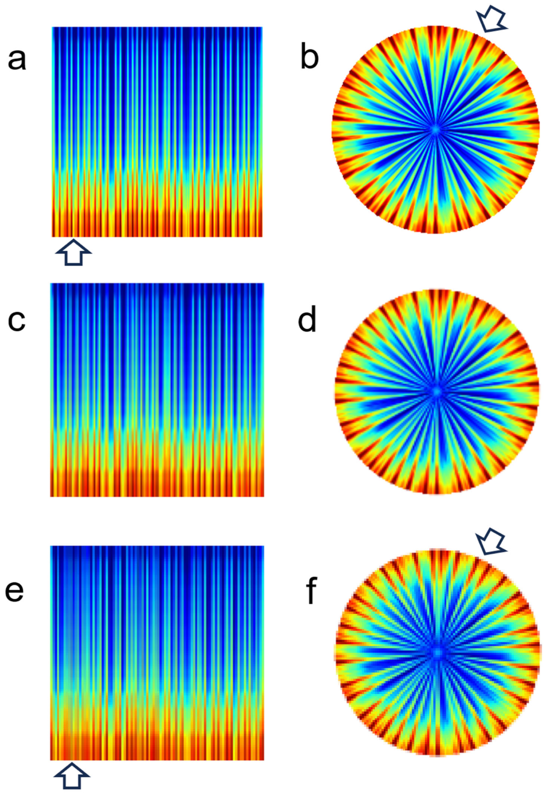
• We demonstrated the advantage of polar-transformed ECG spectrograms in approximately 30 s ECG signals compared to conventional rectangular spectrograms.
• We investigated the effects of image resolution on visualization quality in both rectangular and polar spectrograms.
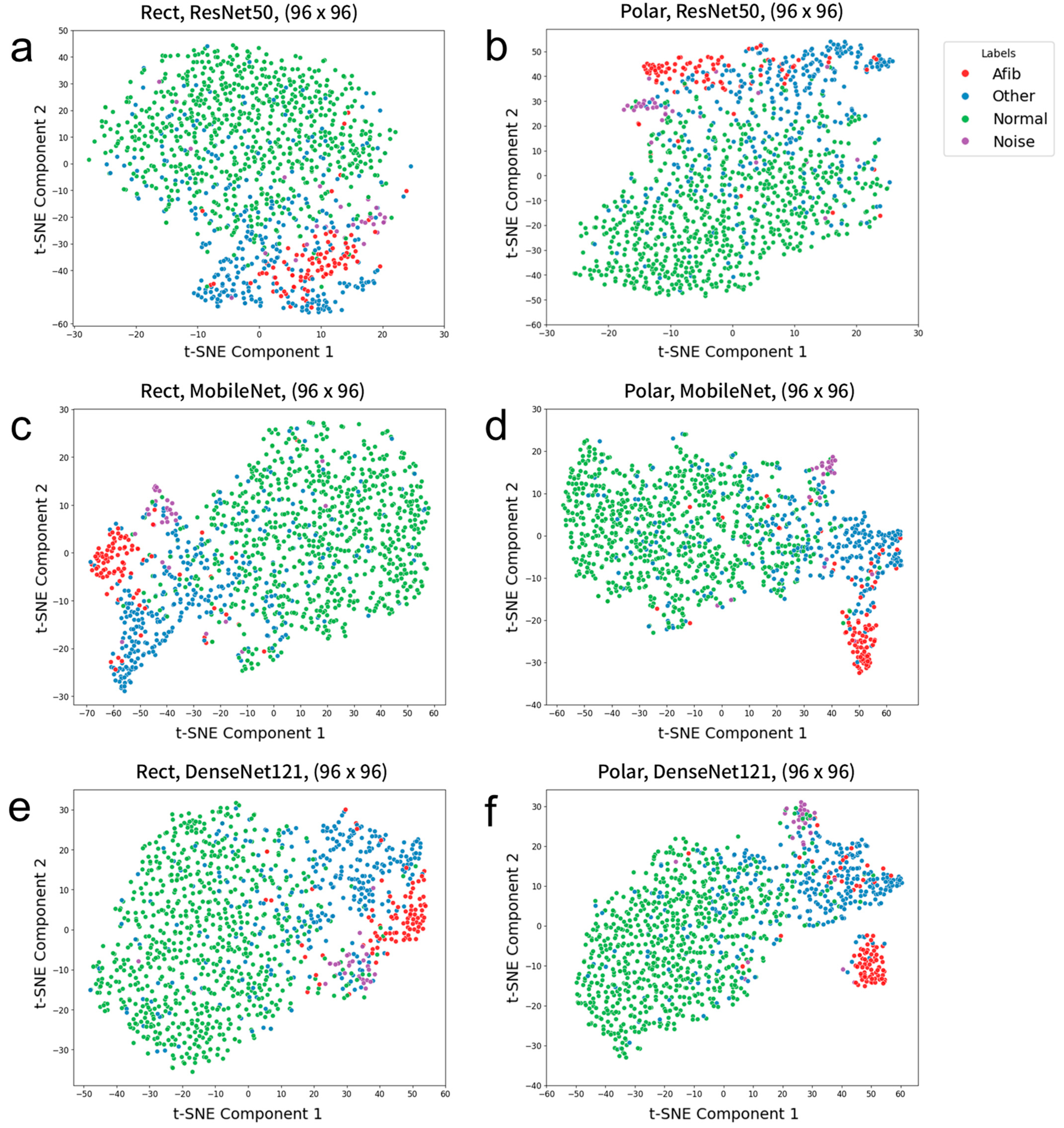
• We assessed the effects of image resolution on deep CNN prediction performance for both rectangular and polar spectrograms.

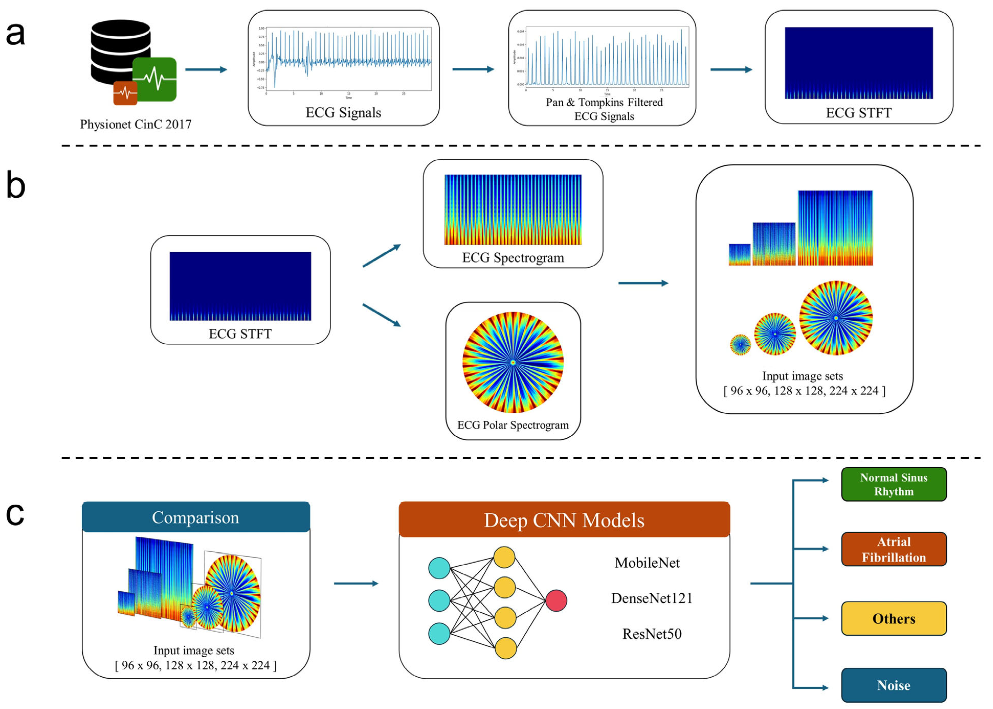
2. Materials and Methods

Figure 1 illustrates a flowchart of our study, which consists of three stages. In the first stage, ECG time series signals underwent preprocessing to produce ECG spectrograms (Figure 1a). In the second stage, logarithmic transformations were applied to the ECG spectrograms, and both rectangular and polar spectrograms were generated along with their corresponding class labels to serve as input data for developing and evaluating the deep learning classifier models (Figure 1b,c).

2.1. Data

ECG data utilized in this study were provided by the PhysioNet/CinC Challenge 2017 (https://physionet.org/content/challenge-2017/1.0.0 (accessed on 6 June 2025)) [31]. The dataset comprised single-lead ECG waveforms with 8528 data samples with the median duration of 30 s. Each recording was categorized into one of four classes: normal sinus rhythm, atrial fibrillation (Afib), other rhythm, or noise (too noisy to classify). The “other rhythm” category included all arrhythmic heartbeats excluding atrial fibrillation.

2.2. Preprocessing of ECG Signals

For ECG signal preprocessing, the Pan–Tompkins (P-T) algorithm [32] was employed, which utilizes a series of low-pass, high-pass, and derivative filters to remove background noise and improve the detection of heartbeat frequency. After the preprocessing, the output signal retained the frequency content of the ECG signal, while background signals irrelevant to the QRS detection were removed. The P-T algorithm is effective for identifying abnormalities in heart rhythm, but it can result in the loss of signals within the R-R intervals, potentially reducing the accuracy in detecting certain heart diseases such as myocardial infarction or hypertrophic cardiomyopathy.

We computed short-time Fourier transform (STFT) on the ECG signal and applied logarithmic transformation to obtain the final spectrograms. We used the stft() function from the SciPy library of the Python programming language (version 3.11) to generate spectrograms [33]. The length of each segment was set to 64 samples, and the number of samples to overlap between segments was set to 32 samples.

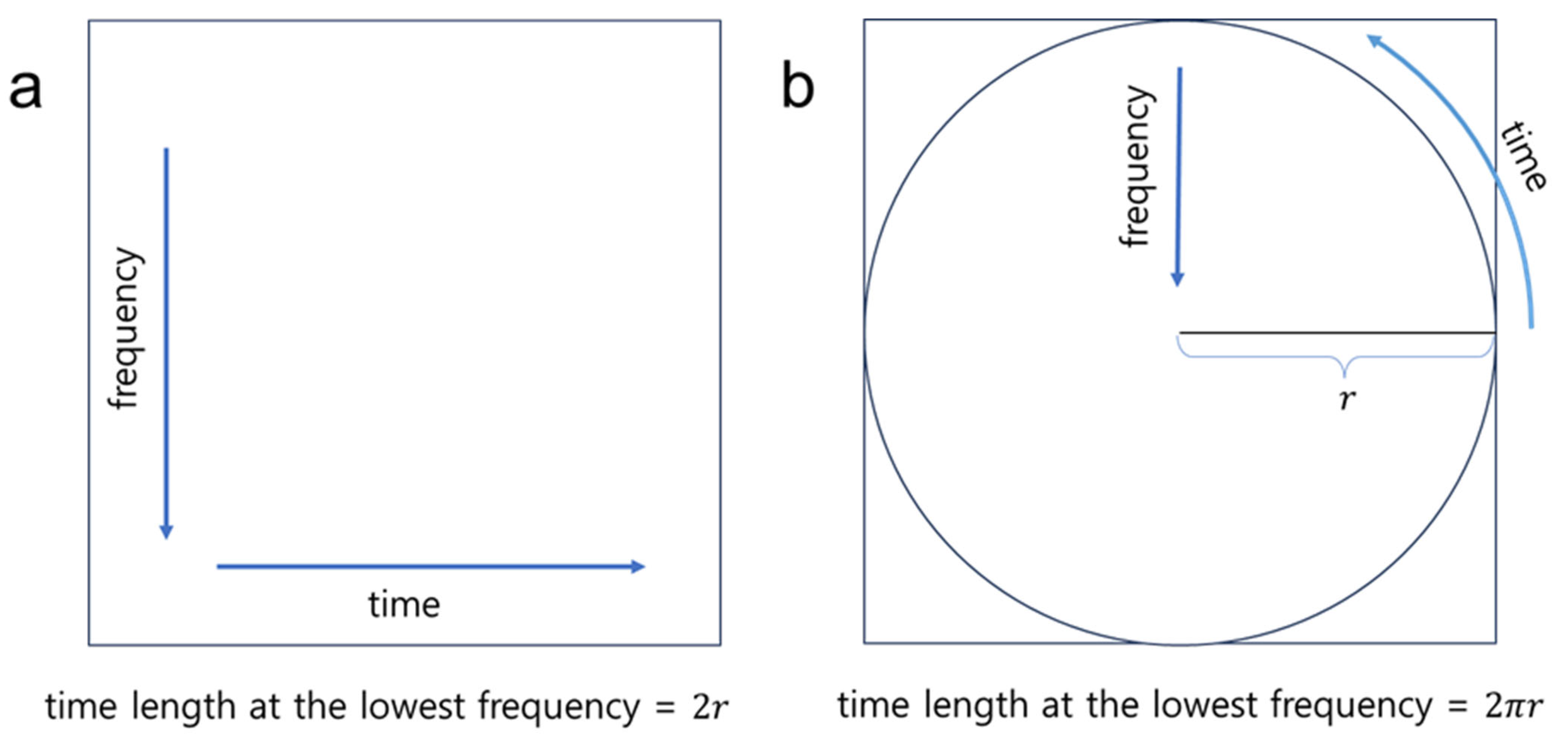
2.3. Polar Transformation

We first mapped the 2D spectrograms to polar coordinates [25]. The resulting scatter plots had unfilled spaces. We used linear interpolation to fill these gaps and obtained the polar-transformed spectrogram images [34]. After interpolation, the polar-transformed spectrogram images exhibited a densely spaced, high-intensity low-frequency region. We implemented a reverse polar transformation, which resulted in wider spacing between peaks in the low-frequency region. The reverse polar transformation is advantageous over the non-reverse polar transformation. With the reverse polar transformation, the low frequency region is located in the periphery of the polar space so that it enhances the distinction between atrial fibrillation (AF) and normal sinus rhythm signals. The polar-transformed images were colored using the “jet” colormap, which shows a color spectrum from blue to red. Image intensity values were rescaled to the range [0, 255] as unsigned 8 bit integers, and images were saved in .png format for subsequent deep learning model development and testing.

Figure 2 compares the rectangular and polar spectrogram layouts. Given identical image dimensions ($2r$ x $2r$), the polar spectrogram (Figure 2b) covers a greater distance (i.e., $2\pi r$ vs. $2r$) at the lowest frequency compared to the conventional rectangular spectrogram (Figure 2a). Note that the four corners in Figure 2b remain empty in the polar spectrogram representation.

2.4. Deep Learning

From the total of 8528 ECG recordings, 5977 with a duration of 30 s were selected for training, validation, and testing of deep CNN models. Polar-transformed spectrograms from 4781 recordings formed the model development group, and polar-transformed spectrograms from 1196 recordings were reserved for testing. The number of recordings in each class for the model development and test groups is summarized in

Table 1. Number of recordings for model development and test.

Class	Model Development	Test
Atrial fibrillation (Afib)	409	90
Normal sinus rhythm	2924	754
Other rhythm	1352	323
Noise	96	29
Total	4781	1196

. Data augmentation schemes were not utilized to address class imbalance. From the model development group, a five-fold cross validation was performed to train and validate five deep CNN models. The deep CNN models were implemented using the Keras library [35]. Pretrained MobileNet [36], ResNet50 [12], and DenseNet121 [37] models, which were pretrained with the ImageNet dataset [14], served as baseline feature extractors. Their weights were frozen during model training. The features extracted using the pretrained models underwent global average pooling (GAP) [38] followed by fully connected layers. The output was classified into one of four categories: atrial fibrillation, normal sinus rhythm, other rhythm, or noise. The Adam optimizer [39] was used during training with sparse categorical cross-entropy as the loss function. Training and validation accuracy were monitored at every epoch.

Each input image was resized to dimensions of 224 × 224 × 3, which is the default setting for the Keras deep learning library. After experimenting with various learning rate values, the learning rate was set to 0.001. Training and validation were performed for up to 50 epochs, and model parameters were saved at each epoch. For each fold, we chose the epoch showing the highest validation accuracy.

2.5. Evaluation

SSIM (Structural Similarity Index Measure) and PSNR (Peak Signal-to-Noise Ratio) were used to objectively evaluate image quality in rectangular and polar-transformed spectrograms. SSIM assesses image similarity by evaluating luminance, contrast, and structural similarity between two images [40], with values closer to 1.0 indicating greater similarity. PSNR calculates the mean square error between two images [40], with higher PSNR values indicating better image quality. For calculating SSIM and PSNR for images sized 128 × 128 and 96 × 96, we used the 224 × 224 images as reference images. A two-sample unpaired t test was performed to determine if the rectangular and polar SSIM or PSNR values are significantly different.

Deep learning training was conducted on a Windows PC (12th Gen Intel^® Core™ i9-12900K, 32 GB RAM (Intel, Santa Clara, CA, USA), and NVIDIA GeForce RTX 3080 with 10 GB memory (Nvidia, Santa Clara, CA, USA)). For each deep learning model, we compared two schemes: (A) rectangular spectrograms and (B) polar-transformed spectrograms, each processed by the P-T method. We tested three prediction methods: MobileNet, ResNet50, and DenseNet121, with final predictions based on soft-voting across five-fold cross-validation.

The Scikit-learn library was used to calculate F1-score, precision, recall, accuracy, and confusion matrices [41]. For a given class c, precision ($P_c$), recall ($R_c$), and F1-score (${F1}_c$) are defined as follows:

$$P_c={\displaystyle \frac{{TP}_c}{{TP}_c+{FP}_c}}$$

(1)

$$R_c={\displaystyle \frac{{TP}_c}{{TP}_c+{FN}_c}}$$

(2)

$${F1}_c={\displaystyle \frac{2\times P_c\times R_c}{P_c+R_c}}$$

(3)

${TP}_c$, ${FN}_c$, and ${FP}_c$ represent the number of true positives, false negatives, and false positives for class c, respectively.

Since our study deals with a multi-class classification problem, we adopted macro-average calculations for the evaluation. The noise class was excluded for the calculation of F1-score according to the PhysioNet/CinC Challenge 2017 guidelines. Thus, we calculated the macro F1-score as follows:

$$F1={\displaystyle \frac{{F1}_N+{F1}_A+{F1}_O}{3}}.$$

(4)

The accuracy score was calculated as:

$$\mathrm{A}\mathrm{c}\mathrm{c}={\displaystyle \frac{\mathrm{N}\mathrm{u}\mathrm{m}\mathrm{b}\mathrm{e}\mathrm{r} \mathrm{o}\mathrm{f} \mathrm{c}\mathrm{o}\mathrm{r}\mathrm{r}\mathrm{e}\mathrm{c}\mathrm{t} \mathrm{p}\mathrm{r}\mathrm{e}\mathrm{d}\mathrm{i}\mathrm{c}\mathrm{t}\mathrm{i}\mathrm{o}\mathrm{n}\mathrm{s}}{\mathrm{T}\mathrm{o}\mathrm{t}\mathrm{a}\mathrm{l} \mathrm{n}\mathrm{u}\mathrm{m}\mathrm{b}\mathrm{e}\mathrm{r} \mathrm{o}\mathrm{f} \mathrm{s}\mathrm{a}\mathrm{m}\mathrm{p}\mathrm{l}\mathrm{e}\mathrm{s}}}.$$

(5)

3. Results

Figure 3 compares rectangular and polar spectrograms illustrating the effect of image resolution on image quality for normal sinus rhythm. As image resolution decreases, spacing between adjacent R-R intervals becomes blurrier in both rectangular and polar spectrograms. Polar-transformed spectrograms (Figure 3b,d,f) exhibit wider spacing between adjacent R-R intervals compared to rectangular spectrograms (Figure 3a,c,e).

In

Table 2. Quantitative comparisons of spectrogram image quality.

Image Dimensions	Metric	Rect	Polar	p-Value
128 × 128	SSIM	0.748 ± 0.053	0.880 ± 0.012	<0.001
	PSNR	17.20 ± 1.37 (dB)	21.05 ± 1.01 (dB)	<0.001
96 × 96	SSIM	0.576 ± 0.081	0.790 ± 0.019	<0.001
	PSNR	14.94 ± 1.43 (dB)	18.59 ± 1.01 (dB)	<0.001

, SSIM and PSNR values were compared between rectangular and polar-transformed spectrograms. We considered all rectangular and polar spectrogram images for evaluation. As can be seen from Table 2, polar-transformed images exhibited higher SSIM and PSNR values compared to rectangular images across all image resolutions (p-value < 0.001). Although lower image resolutions resulted in decreased SSIM and PSNR values for both polar and rectangular spectrograms, polar-transformed spectrograms maintained superior image quality relative to rectangular spectrograms.

Figure 4 compares rectangular and polar spectrograms illustrating the impact of image resolution on image quality for atrial fibrillation. At high resolutions (224 × 224), both rectangular and polar spectrograms clearly distinguish adjacent R-R intervals (Figure 4a,b, arrows). However, at lower resolutions (96 × 96), the polar spectrogram (Figure 4f, arrow) maintains distinguishable spacing between adjacent R-R intervals, while the rectangular spectrogram (Figure 4e, arrow) does not appear distinguishable.

Table 3. Comparison of model capacity and feature map dimensions for three different input image dimensions.

Baseline Network	Input Image Dimensions	The Number of Weight/Bias Parameters in the Baseline network	The Number of Weight/Bias Parameters in the Dense Layers	Feature Map Dimensions (After the First Layer of the Baseline Network)	Feature Map Dimensions (After the Last Layer of the Baseline Network)
ResNet50	96 × 96	23,587,712	23,719,364	(64, 48, 48)	(2048, 3, 3)
	128 × 128	23,587,712	23,719,364	(64, 64, 64)	(2048, 4, 4)
	224 × 224	23,587,712	23,719,364	(64, 112, 112)	(2048, 7, 7)
MobileNet	96 × 96	3,228,864	3,294,980	(32, 48, 48)	(1024, 3, 3)
	128 × 128	3,228,864	3,294,980	(32, 64, 64)	(1024, 4, 4)
	224 × 224	3,228,864	3,294,980	(32, 112, 112)	(1024, 7, 7)
DenseNet121	96 × 96	7,037,504	7,103,620	(64, 48, 48)	(1024, 3, 3)
	128 × 128	7,037,504	7,103,620	(64, 64, 64)	(1024, 4, 4)
	224 × 224	7,037,504	7,103,620	(64, 112, 112)	(1024, 7, 7)

summarizes changes in weight/bias parameters and feature map dimensions across various input image sizes for each baseline network. Given the baseline network, the number of parameters remained constant regardless of input image size, while feature map dimensions decreased by 3/7 when image dimensions changed from 224 to 96. Training deep neural networks with 96 × 96 images was approximately 2–3 times faster compared to training with 224 × 224 images. The consistent number of parameters in dense layers across varying image sizes was due to the use of Global Average Pooling (GAP) layers just after the extraction of features at the penultimate layer of the baseline network.

Table 4. Prediction results on test data.

Baseline Network	Input Image Dimensions	Type	F1A	F1N	F1O	Macro F1-Score	Macro Precision	Macro Recall	Accuracy
ResNet50	96 × 96	Rect	0.6338	0.8879	0.6401	0.7206	0.6727	0.8092	0.8743
		Polar	0.7681	0.7284	0.6503	0.7681	0.7284	0.8283	0.8820
	128 × 128	Rect	0.7058	0.9072	0.6938	0.7690	0.7283	0.8307	0.8937
		Polar	0.7483	0.8901	0.6531	0.7638	0.7638	0.8206	0.8806
	224 × 224	Rect	0.7619	0.9100	0.7338	0.8019	0.7791	0.8301	0.9025
		Polar	0.7607	0.9052	0.7069	0.7909	0.8299	0.7617	0.8931
MobileNet	96 × 96	Rect	0.7354	0.8895	0.6432	0.7560	0.7151	0.8202	0.8797
		Polar	0.7034	0.8920	0.6505	0.7486	0.6989	0.8355	0.8806
	128 × 128	Rect	0.7600	0.9052	0.7164	0.7930	0.7456	0.8646	0.8974
		Polar	0.7625	0.8903	0.6857	0.7795	0.7521	0.8155	0.8843
	224 × 224	Rect	0.8275	0.9148	0.7390	0.8271	0.8049	0.8601	0.9103
		Polar	0.8068	0.9001	0.6967	0.7968	0.7786	0.8375	0.8943
DenseNet121	96 × 96	Rect	0.7058	0.8928	0.7012	0.7666	0.7375	0.8110	0.8846
		Polar	0.7382	0.8970	0.7091	0.7814	0.7431	0.8422	0.8903
	128 × 128	Rect	0.7600	0.9052	0.6987	0.7880	0.7365	0.8741	0.8977
		Polar	0.7790	0.9079	0.6929	0.7933	0.7678	0.8339	0.8983
	224 × 224	Rect	0.8284	0.9150	0.7529	0.8321	0.8069	0.8641	0.9117
		Polar	0.8132	0.9179	0.7079	0.8238	0.8488	0.7841	0.8993

summarizes the prediction performance of various deep CNN models on test data. Polar spectrogram results showed performance comparable to rectangular spectrogram results. For example, at the 96 × 96 image resolution using ResNet50, polar spectrograms achieved a higher macro F1-score (0.7681) compared to rectangular spectrograms (0.7206). When DenseNet121, which produced the highest macro F1-scores at 224 × 224 resolution, was used at 96 × 96 resolution, polar spectrograms consistently showed superior performance across all metrics compared to rectangular spectrograms.

Figure 5 presents t-Distributed Stochastic Neighbor Embedding (t-SNE) visualizations of the penultimate feature distributions. Averaged penultimate features from the five cross-validated models were used as input to TSNE’s fit_transfrom() function in Scikit-Learn. The sample distributions indicate that the polar spectrograms are on par with rectangular spectrograms across all three models. Notably, polar spectrogram samples exhibited tighter clustering compared to rectangular spectrogram samples, as observed with DenseNet121 (Figure 5e,f).

Figure 6 compares confusion matrices for test data predictions using polar and rectangular spectrograms with the DenseNet121 model at various input dimensions. For the normal sinus rhythm and other rhythm classes, the prediction performances of polar and rectangular spectrogram models are comparable. However, for the atrial fibrillation class at 96 × 96 resolution, the polar spectrogram model demonstrates slightly superior prediction performance compared to the rectangular spectrogram model (compare Figure 6e,f).

4. Discussion

We demonstrated the comparison of polar-transformed spectrograms with conventional rectangular spectrograms in terms of visual appearance and deep-leaning-based prediction performance. Polar-transformed spectrograms offer significant advantages over conventional rectangular spectrograms in clearly resolving R-R intervals at lower image resolutions. Furthermore, deep-learning-based arrhythmia prediction performance using polar-transformed spectrograms was comparable to rectangular spectrograms.

A limitation of current approach with polar-transformed spectrograms is the use of the fixed temporal duration (30 s). However, this is a proof-of-concept study, focusing on the advantages of polar-transformed spectrograms. The polar representation itself cannot reveal the temporal duration. As a result, unless the temporal duration of ECG signals is fixed, it is challenging to distinguish between conditions like bradycardia or tachycardia and normal sinus rhythm. It is worth investigating the effectiveness of flexible temporal duration in polar-transformed images for the identification of cardiac arrhythmia. For example, one can embed temporal duration into one of the four corners in the polar-transformed image or use multi-modal inputs by incorporating the temporal duration as an attribute in the neural network.

As the number of samples (i.e., temporal duration of the ECG signal) increases, it becomes difficult to visualize the R-R intervals even in polar-transformed spectrograms, although polar spectrograms are superior to rectangular spectrograms in resolving the R-R intervals given the same image size. Hence, optimal selection of temporal duration for polar image generation may be necessary by taking into account a trade-off between image resolution and temporal duration in ECG signals, when adopting polar representations in the continuous monitoring of cardiac rhythm abnormality. It may be desirable to generate a video that contains frames of polar-transformed spectrograms.

On-device computing with deep learning has drawn a significant degree of attention in the research community since it alleviates the burden of cloud computing by locally processing and analyzing the sensors’ data [42]. However, on-device computing is resource-constrained, and deep learning on edge devices requires lightweight architectures with lower precision (i.e., fewer bits per weight, post-training quantization from float32 to uint8 type) and fewer network connections (i.e., pruning) [42]. Recent studies investigated the comparison of various model architectures with regard to prediction accuracy and memory usage [43]. Quantitative evaluation of memory usage, inference speed, and power consumption on actual edge devices using polar-transformed spectrograms represent important directions for future research.

5. Conclusions

This study investigated the potential benefits of polar-transformed ECG spectrograms compared to conventional rectangular ECG spectrograms for the visualization and deep-learning-based prediction of cardiac arrhythmias. Polar-transformed spectrograms provided improved visualization of R-R intervals, particularly at lower image resolutions, compared to conventional rectangular spectrograms. Moreover, deep learning prediction performance using polar-transformed spectrograms was comparable to that using conventional rectangular spectrograms. The findings of this simulation study suggest that polar-transformation could be effectively utilized in edge computing scenarios, where reduced computing resources such as memory and power consumption are desirable.

References

1. Siontis, K.C.; Noseworthy, P.A.; Attia, Z.I.; Friedman, P.A. Artificial intelligence-enhanced electrocardiography in cardiovascular disease management. Nat. Rev. Cardiol. 2021, 18, 465–478. [Google Scholar] [CrossRef] [PubMed]
2. Joglar, J.A.; Chung, M.K.; Armbruster, A.L.; Benjamin, E.J.; Chyou, J.Y.; Cronin, E.M.; Deswal, A.; Eckhardt, L.L.; Goldberger, Z.D.; Gopinathannair, R.; et al. 2023 ACC/AHA/ACCP/HRS Guideline for the Diagnosis and Management of Atrial Fibrillation: A Report of the American College of Cardiology/American Heart Association Joint Committee on Clinical Practice Guidelines. Circulation 2024, 149, e1–e156. [Google Scholar] [CrossRef] [PubMed]
3. Sanna, T.; Diener, H.C.; Passman, R.S.; Crystal, A.F.S.C. Cryptogenic stroke and atrial fibrillation. N. Engl. J. Med. 2014, 371, 1261. [Google Scholar] [CrossRef] [PubMed]
4. Attia, Z.I.; Noseworthy, P.A.; Lopez-Jimenez, F.; Asirvatham, S.J.; Deshmukh, A.J.; Gersh, B.J.; Carter, R.E.; Yao, X.; Rabinstein, A.A.; Erickson, B.J.; et al. An artificial intelligence-enabled ECG algorithm for the identification of patients with atrial fibrillation during sinus rhythm: A retrospective analysis of outcome prediction. Lancet 2019, 394, 861–867. [Google Scholar] [CrossRef] [PubMed]
5. Ansari, M.Y.; Qaraqe, M.; Charafeddine, F.; Serpedin, E.; Righetti, R.; Qaraqe, K. Estimating age and gender from electrocardiogram signals: A comprehensive review of the past decade. Artif. Intell. Med. 2023, 146, 102690. [Google Scholar] [CrossRef] [PubMed]
6. Ebrahimi, Z.; Loni, M.; Daneshtalab, M.; Gharehbaghi, A. A review on deep learning methods for ECG arrhythmia classification. Expert Syst. Appl. X 2020, 7, 100033. [Google Scholar] [CrossRef]
7. Kumar, A.; Kumar, S.A.; Dutt, V.; Dubey, A.K.; García-Díaz, V. IoT-based ECG monitoring for arrhythmia classification using Coyote Grey Wolf optimization-based deep learning CNN classifier. Biomed. Signal Process. Control 2022, 76, 103638. [Google Scholar] [CrossRef]
8. Hannun, A.Y.; Rajpurkar, P.; Haghpanahi, M.; Tison, G.H.; Bourn, C.; Turakhia, M.P.; Ng, A.Y. Cardiologist-level arrhythmia detection and classification in ambulatory electrocardiograms using a deep neural network. Nat. Med. 2019, 25, 65–69. [Google Scholar] [CrossRef] [PubMed]
9. Tesfai, H.; Saleh, H.; Al-Qutayri, M.; Mohammad, M.B.; Tekeste, T.; Khandoker, A.; Mohammad, B. Lightweight Shufflenet Based CNN for Arrhythmia Classification. IEEE Access 2022, 10, 111842–111854. [Google Scholar] [CrossRef]
10. Cao, P.; Li, X.Y.; Mao, K.D.; Lu, F.; Ning, G.M.; Fang, L.P.; Pan, Q. A novel data augmentation method to enhance deep neural networks for detection of atrial fibrillation. Biomed. Signal Process. Control 2020, 56, 101675. [Google Scholar] [CrossRef]
11. Song, M.S.; Lee, S.B. Comparative study of time-frequency transformation methods for ECG signal classification. Front. Signal Process. 2024, 4, 1322334. [Google Scholar] [CrossRef]
12. He, K.; Zhang, X.; Ren, S.; Sun, J. Identity mappings in deep residual networks. In Proceedings of the Computer Vision–ECCV 2016: 14th European Conference, Amsterdam, The Netherlands, 11–14 October 2016; Proceedings, Part IV 14. pp. 630–645. [Google Scholar]
13. Alzubaidi, L.; Zhang, J.L.; Humaidi, A.J.; Al-Dujaili, A.; Duan, Y.; Al-Shamma, O.; Santamaría, J.; Fadhel, M.A.; Al-Amidie, M.; Farhan, L. Review of deep learning: Concepts, CNN architectures, challenges, applications, future directions. J. Big Data-Ger. 2021, 8, 53. [Google Scholar] [CrossRef] [PubMed]
14. Deng, J.; Dong, W.; Socher, R.; Li, L.J.; Li, K.; Li, F.F. ImageNet: A Large-Scale Hierarchical Image Database. In Proceedings of the 2009 IEEE Conference on Computer Vision and Pattern Recognition, Miami, FL, USA, 20–25 June 2009; pp. 248–255. [Google Scholar] [CrossRef]
15. Al Rahhal, M.M.; Bazi, Y.; Al Zuair, M.; Othman, E.; BenJdira, B. Convolutional Neural Networks for Electrocardiogram Classification. J. Med. Biol. Eng. 2018, 38, 1014–1025. [Google Scholar] [CrossRef]
16. Eltrass, A.S.; Tayel, M.B.; Ammar, A. A new automated CNN deep learning approach for identification of ECG congestive heart failure and arrhythmia using constant-Q non-stationary Gabor transform. Biomed. Signal Process. 2021, 65, 102326. [Google Scholar] [CrossRef]
17. Çinar, A.; Tuncer, S.A. Classification of normal sinus rhythm, abnormal arrhythmia and congestive heart failure ECG signals using LSTM and hybrid CNN-SVM deep neural networks. Comput. Methods Biomech. Biomed. Eng. 2021, 24, 203–214. [Google Scholar] [CrossRef] [PubMed]
18. Huang, J.S.; Chen, B.Q.; Yao, B.; He, W.P. ECG Arrhythmia Classification Using STFT-Based Spectrogram and Convolutional Neural Network. IEEE Access 2019, 7, 92871–92880. [Google Scholar] [CrossRef]
19. Khorrami, H.; Moavenian, M. A comparative study of DWT, CWT and DCT transformations in ECG arrhythmias classification. Expert Syst. Appl. 2010, 37, 5751–5757. [Google Scholar] [CrossRef]
20. Krak, I.; Stelia, O.; Pashko, A.; Efremov, M.; Khorozov, O. Electrocardiogram classification using wavelet transformations. In Proceedings of the 2020 IEEE 15th International Conference on Advanced Trends in Radioelectronics, Telecommunications and Computer Engineering (TCSET), Online, 25–29 February 2020; pp. 930–933. [Google Scholar]
21. Li, C.; Zheng, C.; Tai, C. Detection of ECG characteristic points using wavelet transforms. IEEE Trans. Biomed. Eng. 1995, 42, 21–28. [Google Scholar] [CrossRef] [PubMed]
22. Mewada, H.; Pires, I.M. Electrocardiogram signal classification using lightweight DNN for mobile devices. Procedia Comput. Sci. 2023, 224, 558–564. [Google Scholar] [CrossRef]
23. Ozaltin, O.; Yeniay, O. A novel proposed CNN–SVM architecture for ECG scalograms classification. Soft Comput. 2023, 27, 4639–4658. [Google Scholar] [CrossRef] [PubMed]
24. Rashidah Funke, O.; Ibrahim, S.N.; Ani Liza, A.; Hunain, A. Classification of ECG signals for detection of arrhythmia and congestive heart failure based on continuous wavelet transform and deep neural networks. Indones. J. Electr. Eng. Comput. Sci. 2021, 22, 1520–1528. [Google Scholar] [CrossRef]
25. Kwon, D.; Kang, H.; Lee, D.; Kim, Y.C. Deep learning-based prediction of atrial fibrillation from polar transformed time-frequency electrocardiogram. PLoS ONE 2025, 20, e0317630. [Google Scholar] [CrossRef] [PubMed]
26. Zhivomirov, H. A novel visual representation of the signals in the time-frequency domain. UPB Sci. Bull. Ser. C Electr. Eng. Comput. Sci. 2018, 80, 75–84. [Google Scholar]
27. Alqudah, A.M.; Alqudah, A. Deep learning for single-lead ECG beat arrhythmia-type detection using novel iris spectrogram representation. Soft Comput. 2022, 26, 1123–1139. [Google Scholar] [CrossRef]
28. Zyout, A.; Alquran, H.; Mustafa, W.A.; Alqudah, A.M. Advanced Time-Frequency Methods for ECG Waves Recognition. Diagnostics 2023, 13, 308. [Google Scholar] [CrossRef] [PubMed]
29. Obeidat, Y.; Alqudah, A.M. A hybrid lightweight 1D CNN-LSTM architecture for automated ECG beat-wise classification. Trait. Du Signal 2021, 38, 1281–1291. [Google Scholar] [CrossRef]
30. Banerjee, R.; Ghose, A. A Light-Weight Deep Residual Network for Classification of Abnormal Heart Rhythms on Tiny Devices. In Proceedings of the Joint European Conference on Machine Learning and Knowledge Discovery in Databases, Turin, Italy, 18–22 September 2023; Volume 1753, pp. 317–331. [Google Scholar] [CrossRef]
31. Clifford, G.D.; Liu, C.; Moody, B.; Li-wei, H.L.; Silva, I.; Li, Q.; Johnson, A.; Mark, R.G. AF classification from a short single lead ECG recording: The PhysioNet/computing in cardiology challenge 2017. In Proceedings of the 2017 Computing in Cardiology (CinC), Rennes, France, 24–27 September 2017; pp. 1–4. [Google Scholar]
32. Pan, J.; Tompkins, W.J. A real-time QRS detection algorithm. IEEE Trans. Biomed. Eng. 1985, 32, 230–236. [Google Scholar] [CrossRef] [PubMed]
33. Virtanen, P.; Gommers, R.; Oliphant, T.E.; Haberland, M.; Reddy, T.; Cournapeau, D.; Burovski, E.; Peterson, P.; Weckesser, W.; Bright, J.; et al. SciPy 1.0: Fundamental algorithms for scientific computing in Python. Nat. Methods. 2020, 17, 352. [Google Scholar] [CrossRef] [PubMed]
34. Jackson, J.I.; Meyer, C.H.; Nishimura, D.G.; Macovski, A. Selection of a convolution function for Fourier inversion using gridding (computerised tomography application). IEEE Trans. Med. Imaging 1991, 10, 473–478. [Google Scholar] [CrossRef] [PubMed]
35. Chollet, F.O. Deep Learning with Python, 2nd ed.; Manning Publications: Shelter Island, NY, USA, 2021; pp. 68–94. [Google Scholar]
36. Howard, A.G.; Zhu, M.; Chen, B.; Kalenichenko, D.; Wang, W.; Weyand, T.; Andreetto, M.; Adam, H. Mobilenets: Efficient convolutional neural networks for mobile vision applications. arXiv 2017, arXiv:1704.04861. [Google Scholar]
37. Huang, G.; Liu, Z.; Van Der Maaten, L.; Weinberger, K.Q. Densely connected convolutional networks. In Proceedings of the IEEE Conference on Computer Vision and Pattern Recognition, Honolulu, HI, USA, 21–26 July 2017; pp. 4700–4708. [Google Scholar]
38. Zhou, B.; Khosla, A.; Lapedriza, A.; Oliva, A.; Torralba, A. Learning deep features for discriminative localization. In Proceedings of the Conference on Computer Vision and Pattern Recognition, Las Vegas, NV, USA, 27–30 June 2016; pp. 2921–2929. [Google Scholar]
39. Kingma, D.P.; Ba, J. Adam: A method for stochastic optimization. arXiv 2014, arXiv:1412.6980. [Google Scholar]
40. Hore, A.; Ziou, D. Image quality metrics: PSNR vs. SSIM. In Proceedings of the 2010 20th International Conference on Pattern Recognition, Istanbul, Turkey, 23–26 August 2010; pp. 2366–2369. [Google Scholar]
41. Pedregosa, F.; Varoquaux, G.; Gramfort, A.; Michel, V.; Thirion, B.; Grisel, O.; Blondel, M.; Prettenhofer, P.; Weiss, R.; Dubourg, V. Scikit-learn: Machine learning in Python. J. Mach. Learn. Res. 2011, 12, 2825–2830. [Google Scholar]
42. Merenda, M.; Porcaro, C.; Iero, D. Edge Machine Learning for AI-Enabled IoT Devices: A Review. Sensors 2020, 20, 2533. [Google Scholar] [CrossRef] [PubMed]
43. Rahman, S.; Pal, S.; Yearwood, J.; Karmakar, C. Analysing performances of DL-based ECG noise classification models deployed in memory-constraint IoT-enabled devices. IEEE Trans. Consum. Electron. 2024, 70, 704–714. [Google Scholar] [CrossRef]
Figure 1. Flowchart of our study. (a) Signal preprocessing including Pan–Tompkins ECG signal filtering. (b) Generation of ECG spectrogram and its polar transformation as input to a deep neural network architecture. (c) Deep learning model development and test.
Applsci 15 07980 g001
Figure 2. Illustrative comparison of (a) the rectangular spectrogram and (b) the polar-transformed spectrogram.
Applsci 15 07980 g002
Figure 3. Effect of resolution on image quality—normal sinus rhythm. (a) Rectangular spectrogram at 224 × 224 resolution. (b) Polar spectrogram at 224 × 224 resolution. (c) Rectangular spectrogram at 128 × 128 resolution. (d) Polar spectrogram at 128 × 128 resolution. (e) Rectangular spectrogram at 96 × 96 resolution. (f) Polar spectrogram at 96 × 96 resolution.
Applsci 15 07980 g003
Figure 4. Effect of resolution on image quality—atrial fibrillation. (a) Rectangular spectrogram at 224 × 224 resolution. (b) Polar spectrogram at 224 × 224 resolution. (c) Rectangular spectrogram at 128 × 128 resolution. (d) Polar spectrogram at 128 × 128 resolution. (e) Rectangular spectrogram at 96 × 96 resolution. (f) Polar spectrogram at 96 × 96 resolution.
Applsci 15 07980 g004
Figure 5. t-SNE scatter plots obtained using the (a,b) ResNet50, (c,d) MobileNet, and (e,f) DenseNet121 models for the prediction of four classes using test datasets with the image dimensions of 96 × 96. (a,c,e) Rectangular spectrograms as input. (b,d,f) Polar spectrograms as input.
Applsci 15 07980 g005
Figure 6. Confusion matrices when applying the DenseNet121 models to test data. Deep learning prediction results on polar-transformed spectrogram images when (a) 224 × 224, (c) 128 × 128, and (e) 96 × 96 images were used as input. Deep learning prediction results on rectangular spectrogram images when (b) 224 × 224, (d) 128 × 128, and (f) 96 × 96 images were used as input. A: atrial fibrillation; N: normal sinus rhythm; O: other rhythm; ~: noise.
Applsci 15 07980 g006