Article

Application of Dynamic Time Warping (DTW) in Comparing MRT Signals of Steel Ropes

by
Justyna Tomaszewska
1,*,
Mirosław Witoś
2 and
Jerzy Kwaśniewski
3
1
Faculty of Aviation, Polish Air Force University, Dywizjonu 303 nr 35, 08-521 Dęblin, Poland
2
Air Force Institute of Technology, Ks. Bolesława 6, 01-494 Warszawa, Poland
3
Faculty of Mechanical Engineering and Robotics, AGH University, al. Mickiewicza 30, 30-059 Kraków, Poland
*
Author to whom correspondence should be addressed.
Appl. Sci. 2025, 15(14), 7924; https://doi.org/10.3390/app15147924
Submission received: 30 May 2025 / Revised: 4 July 2025 / Accepted: 10 July 2025 / Published: 16 July 2025
(This article belongs to the Section Aerospace Science and Engineering)

Abstract

Steel wire ropes used in transport and aerospace applications are critical components whose failure can lead to significant safety, operational, and environmental consequences. Current diagnostic practices based on magnetic rope testing (MRT) often suffer from signal misalignment and subjective interpretation, particularly under varying operational conditions or in polymer-impregnated ropes with delayed damage indicators. This study explores the application of the Dynamic Time Warping (DTW) algorithm to enhance the reliability of MRT diagnostics. The research involved analyzing long-term MRT recordings of wire ropes used in mining operations, including different scanning resolutions and signal acquisition methods. A mathematical formulation of DTW is provided along with its implementation code in R and Python. The DTW algorithm was applied to synchronize diagnostic signals with their baseline recordings, as recommended by ISO 4309:2017 and EN 12927:2019 standards. Results show that DTW enables robust alignment of time series with slowly varying spectra, thereby improving the comparability and interpretation of MRT data. This approach reduces the risk of unnecessary rope discard and increases the effectiveness of degradation monitoring. The findings suggest that integrating DTW into existing diagnostic protocols can contribute to safer operation, lower maintenance costs, and reduced environmental impact.

1. Introduction

Steel wire ropes are essential components in vertical and horizontal transport systems including cranes, mine hoists, offshore structures, aircraft arresting systems, and cableways [1]. Their operational reliability directly affects human safety, equipment durability, and economic performance. Among various non-destructive testing (NDT) methods, magnetic rope testing (MRT) remains the most widely adopted diagnostic technique due to its ability to detect internal and external defects without dismantling the rope. Unlike visual inspection, which covers only surface-level damage and ~20% of the rope cross-section, MRT offers a full-profile magnetic assessment and is standardized under several international norms (e.g., ISO 4309:2017 [2], EN 12927:2019 [3]). MRT is relatively cost-effective, robust, and applicable to ropes in a wide range of industrial environments.
gaDespite technological advancements, MRT still suffers from diagnostic uncertainty due to signal degradation caused by rope elongation, external wire abrasion, corrosion, and inconsistent data acquisition settings. Steel wire ropes consist of multiple outer and inner strands, whose surface wear manifests over time through visible damage such as strand flattening or broken wires. The number of broken outer wires is directly correlated with the rope’s consumption level relative to its expected service life [4,5,6]. Figure 1 shows different levels of corrosion observed in ropes exposed to harsh environments.
Corrosion risk is minimized through protective measures such as galvanized coatings with zinc, aluminum, and magnesium (e.g., BEZINAL® 3000) or zinc, aluminum, and sodium (e.g., ZINCAL®); factory lubrication with in-service relubrication; polymer-impregnated strand fills; and polymer sheathing [1,10]. In aggressive conditions, ropes made of corrosion-resistant high-alloy steels (e.g., X5CrNiMo17-12-2, X1CrNiMoCuN20-18-7, X1CrNi25-21) are preferred [EN 10088-1:2005 [11]; EN 10088-5:2009 [12]]. However, these austenitic steels are paramagnetic and therefore not suitable for MRT.
Wear and fatigue are also influenced by structural design, such as the contact type between wires (Figure 2a), compacted strand geometry (Figure 2b), and outer surface construction (Figure 2c). Additional factors include strand core type (Figure 2d–e), motion parameters, and interacting element geometry. These factors help minimize contact stresses, protect against galvanic layer wear, and reduce crack initiation.
During operation, steel wires are subjected to complex stress states caused by repeated bending, torsion, and axial loads. These forces lead to localized strain hardening, fatigue-induced microstructural degradation, and progressive mechanical softening. As the fatigue process evolves, the average tensile strength of the wires decreases—a phenomenon particularly evident in ropes with polymer cores such as the 6 × 36 construction [17]. This mechanical degradation is accompanied by alterations in magnetic properties, including shifts in magnetic permeability and remanence, which further complicate the interpretation of magnetic rope testing (MRT) signals. These combined magneto-mechanical effects reduce the clarity of diagnostic features, especially in advanced rope designs where internal damage may not produce a strong magnetic response.
Laboratory-based empirical formulas (Equation (1)) describe the fatigue life of steel wire ropes under bending in controlled conditions [1]. The rope is described by a MISO (Multi-Input Single-Output) model considering only a single mechanical parameter. However, real-world degradation progresses faster due to variable loads, environmental exposure, and human factors. The adjusted fatigue life considering exploitation quality is given in Equation (2).
g   N = b 0 + b 1 + b 3 · l g D d · l g S d 2 0.4 · l g R o 1770 + b 2 · l g D d + l g f d + l g f L + l g f E
l g   N u = lg N K j e u s e r   o f   r o p e           K j e > 1.0
where bi—constants for the wire ropes of the important rope constructions; fd, fL, and fC—the endurance factors; d [mm]—nominal rope diameter; D [mm]—sheave diameter, S [N]—rope tensile force; R0 [N/mm2]—nominal tensile strength; l [mm]—bending length. During operation, the wires and strands of the rope are subjected to simultaneous bending, torsion, and tension, which is described by a MIMO (Multi-Input Multi-Output) model. Since rope degradation depends on unknown user-specific variables and material scatter, the service life must be treated as a random variable. Thus, the failure risk is defined by Equation (3), in line with ISO/IEC Guide 73:2002.
R i s k = P r o b a b i l i t y   o f   e v e n t   · C o n s e q u e n c e   o f   e v e n t
The safe operation of wire ropes exposed to
  • Corrosion;
  • Premature rust and oxidation;
  • Mechanical wear;
  • Internal and external wire breaks;
  • Fatigue in bends;
  • Tension breaks;
  • Core failure fatigue;
  • Shear breaks;
  • Heat damage;
  • requires continuous technical monitoring. This is mandated by EU legislation [18] and national regulations [19].
Over the past 150 years, the sudden failure of steel wire ropes has led to numerous critical incidents in mine hoists, elevators, cableways, offshore cranes, and suspension bridges. Notable examples include the Robinson Deep Mine disaster [20], the Stresa–Mottarone cable car collapse [21], and the Morbi bridge failure [22,23]. Common causes include undetected corrosion, fatigue degradation, and diagnostic errors linked to limitations of the current inspection techniques or human factors.
In contrast to military systems—where daily inspections and redundancy protocols are enforced—most civilian users rely on periodic MRT or visual checks. However, visual inspections assess only ~20% of the rope’s cross-section, and MRT interpretation can be ambiguous due to signal noise, overlap, and indirect measurement [22,23].
To improve diagnostics, methods such as acoustic emission (AE) [24], ultrasonics [25], FBG strain sensing [26], weak magnetic excitation [27], and modal analysis [28] have been proposed. Still, practical adoption is limited by equipment cost, complexity, and sensitivity to conditions.
Both MRT and MPM share inherent weaknesses: they rely on indirect magnetic symptoms, suffer from defect signal averaging, and depend on operator interpretation. This introduces a trade-off between
  • Type I errors (false positives)—premature rope discard and increased carbon footprint (up to 2300 kg CO2 per ton of steel),
  • Type II errors (false negatives)—missed critical damage with safety risks.
Moreover, advanced MRT algorithms typically focus on localized anomalies like broken wires or pitting corrosion [29]. They rarely address the deeper mechanical changes preceding visible failure such as magnetic permeability shifts, strand rearrangement, or changes in rope geometry due to elongation or compaction. These effects are particularly problematic in polymer-filled and compacted ropes, where progressive elongation during service life alters the relative position of rope segments between inspections. As a result, signal synchronization becomes increasingly unreliable over time, directly impacting discard criteria and diagnostic consistency [16].
To reduce the risk of Type II errors, users apply safety factors (e.g., K > 5 in mining), frequent MRT inspections, and conservative discard rules. Still, unnecessary rope replacements remain common, contributing to excessive material loss and carbon emissions, especially in large-diameter ropes.
Although standards like ISO 4309:2017 and EN 12927:2019 recommend minimum scan resolution (≤1 mm), signal-to-noise thresholds (SNR > 2.0), and baseline comparisons, they do not address how to compensate for rope elongation over time. This directly impacts the consistency of magnetic signatures and undermines comparisons across inspections—particularly in polymer-impregnated ropes.
Recent advances in structural health monitoring (SHM) have increasingly leveraged optical fiber sensing and data-driven modeling techniques for deformation assessment in infrastructure. Ref. [30] developed a distributed optical fiber monitoring system based on BOTDA and fiber Bragg grating (FBG) sensors, enabling 3D tracking of pipeline and soil deformation under lateral displacement and demonstrating effectiveness in recovering strain distribution even under environmental noise. Furthermore, [31] implemented a long-gauge FBG sensing system integrated with STOA-Bi-LSTM-GAN to recover missing data and reconstruct deformation fields with <10% error under data loss conditions. These studies exemplify the increasing capability of advanced SHM methods to detect gradual, distributed damage—insight that directly aligns with our DTW-enhanced MRT approach for early fault detection in wire ropes.
The originality of this work lies in the novel application of the Dynamic Time Warping (DTW) algorithm to the synchronization and differential analysis of low-frequency (LF) magnetic signals obtained during magnetic rope testing (MRT). While DTW is widely used in speech processing, bioinformatics, and time-series clustering, its deployment in rope diagnostics, particularly for compensating signal distortion due to elongation and scan variability, remains unexplored.
The research addresses a key gap in MRT-based diagnostics: the limited ability of traditional signal processing to adapt to resolution degradation, mechanical strain evolution, and internal changes in polymer-impregnated wire ropes. Existing MRT algorithms focus primarily on localized discontinuities such as wire breaks or corrosion pits, whereas our approach enables the detection of broader spectrum shifts and synchronization challenges across repeated scans.
This contribution is especially relevant for steel ropes used in safety-critical applications (e.g., mining, transport, offshore), where long-term signal stability and resolution adaptation are crucial. The method also offers compatibility with standard MRT equipment and is applicable across various software platforms (e.g., R 4.4.2, Python 3.9.21, MATLAB R2024b), enhancing its potential for industry adoption.
The structure of the article includes the following: (1) an introduction and literature review, (2) a theoretical section on MRT signal modeling and DTW implementation, (3) the characterization of rope samples and measurement conditions, and (4) experimental validation using active and archival MRT data, followed by a discussion of the results and practical implications.

2. Materials and Methods
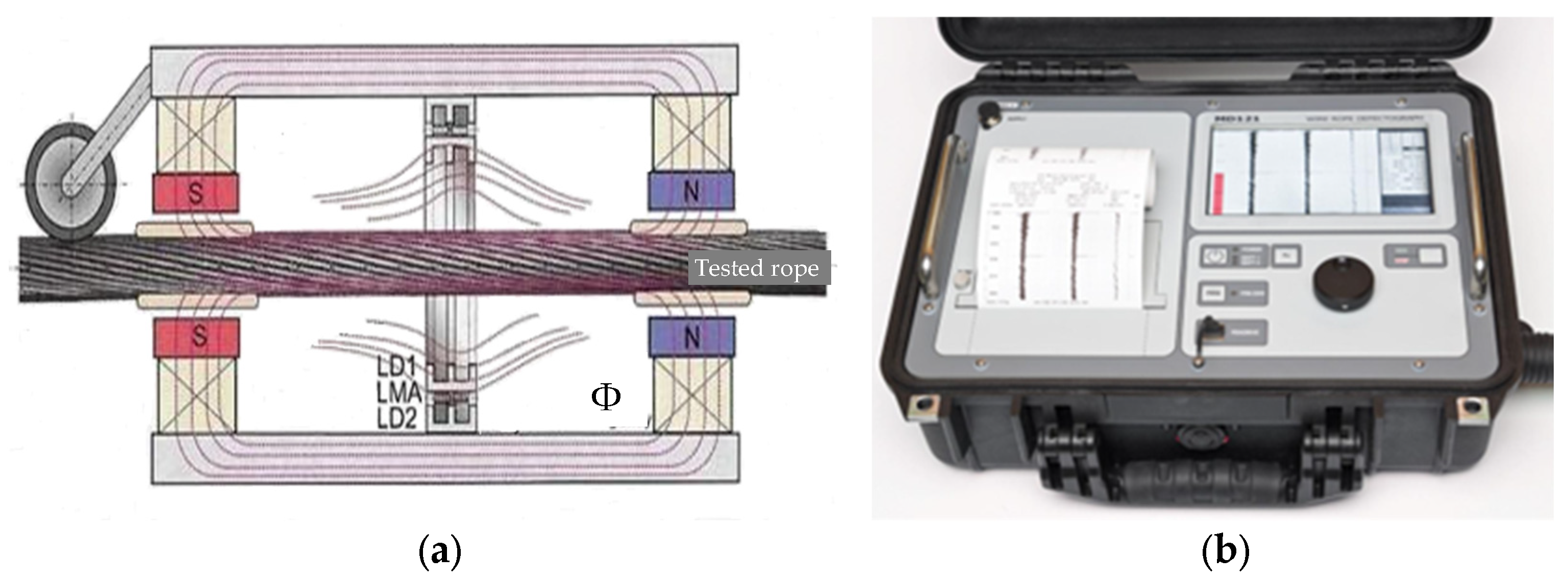
2.1. MRT Methods

Information about the current technical condition of the rope is obtained during non-destructive testing using the MRT magnetic method. Measurement data from MRT tests are recorded by the measurement path containing (Figure 3) the following:
  • A measuring head with
  • the circuit of longitudinal magnetization of a fragment of a steel rope based on permanent magnets and magnetoguides;
  • two searching coils on the E-core, wrapping the tested rope in two different ways, which generate LF1 and LF2 signals (also marked in the literature as LD1 and LD2, local defect) proportional to the speed of changes in the magnetic flux (features of magnetic anomalies) and the location of the defect in the cross-section of the rope, taking into account the influence of the structural features of the E-core and the rope magnetization circuit on the signal spectrum;
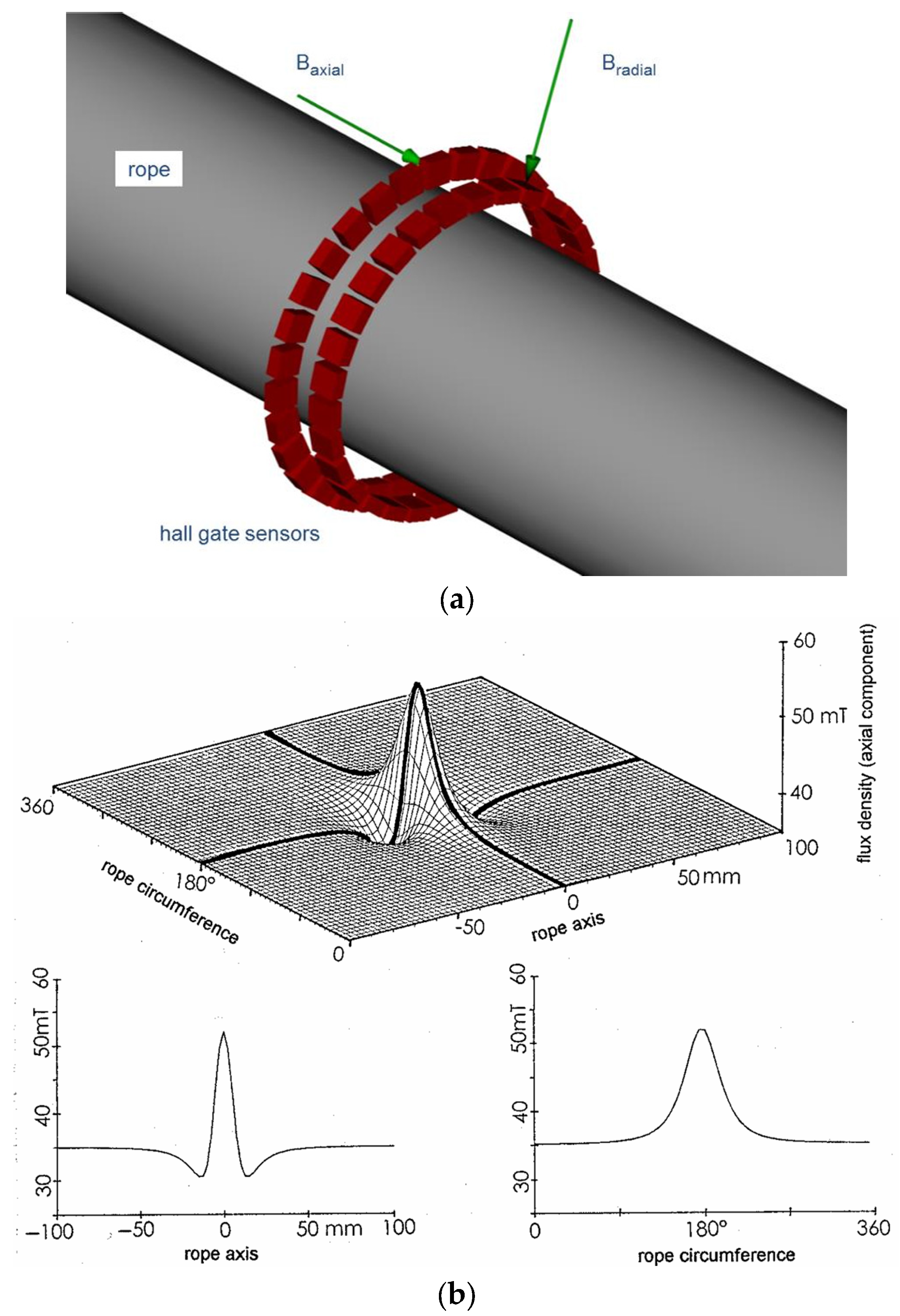
  • two Hall sensors with a magnetic field concentrator located between the coils, which record the scattering field around the rope and generate a resultant LMA signal proportional to the strength of the magnetic field.
  • A defectograph in which
  • the influence of changes in the speed of rope scanning (type from 0.15 m/s to 4 m/s) on the amplitude of LF1 and LF2 signals using the signal from the encoder is compensated;
  • signals  L F 1 , L F 2 , L M A and recording time t are sampled in parallel with a set frequency in the TIMER mode or the resolution of the rope displacement scan in the ENCODER mode;
  • measurement data discrete in time are saved on a non-volatile memory carrier;
  • the course of the recorded time series is illustrated on the screen;
  • measurement data are pre-processed (filtration and calculation of additional variables—rope scanning speed in ENCODER mode, LF1 integrals, defined diagnostic estimates);
  • a simplified analysis of measurement data is carried out according to preset criteria in the time domain or order, including visual comparison of the results with the previous recording (reference result);
  • the function of printing test results on a thermal printer or an external printer is available;
  • data transfer to an external computer (for extended data analysis and data archiving) is carried out using a standard RS-232 or USB 2.0 port.

2.1.1. Numerical Model of Search Coils

Search coils LF1 and LF2—main components of the MRT measurement path—are the generic name of a widespread class of sensors consisting of loops of conducting wire exposed to a magnetic field B and generating an output voltage VC via Faraday’s induction law [33,34]. For a coil, shown in Figure 4a, made with NT closed turns spanning an area A with normal unit vector n and boundary A , the output voltage V c is given by the total rate of change of the linked magnetic flux Φ as in Equation (4). The negative sign (from Lenz’s law) means that the induced electromotive force e m f tends to generate a current which, by the right-hand rule, gives rise to a field opposing the variation in the flux. A typical distribution of the magnetic field in the vicinity of a round-twisted rope is illustrated in Figure 4b. The distribution of the magnetic field contains information about
  • The structural features of the rope—each outer strand generates a clear cyclic change in the magnetic field. Internal and medullary convolutions are also a source of weak cyclic magnetic anomalies.
  • The technical condition of the rope.
V c = d Φ d t = L c d i d t = d d t A B n d A = A B d t n d A A v x B d l
where
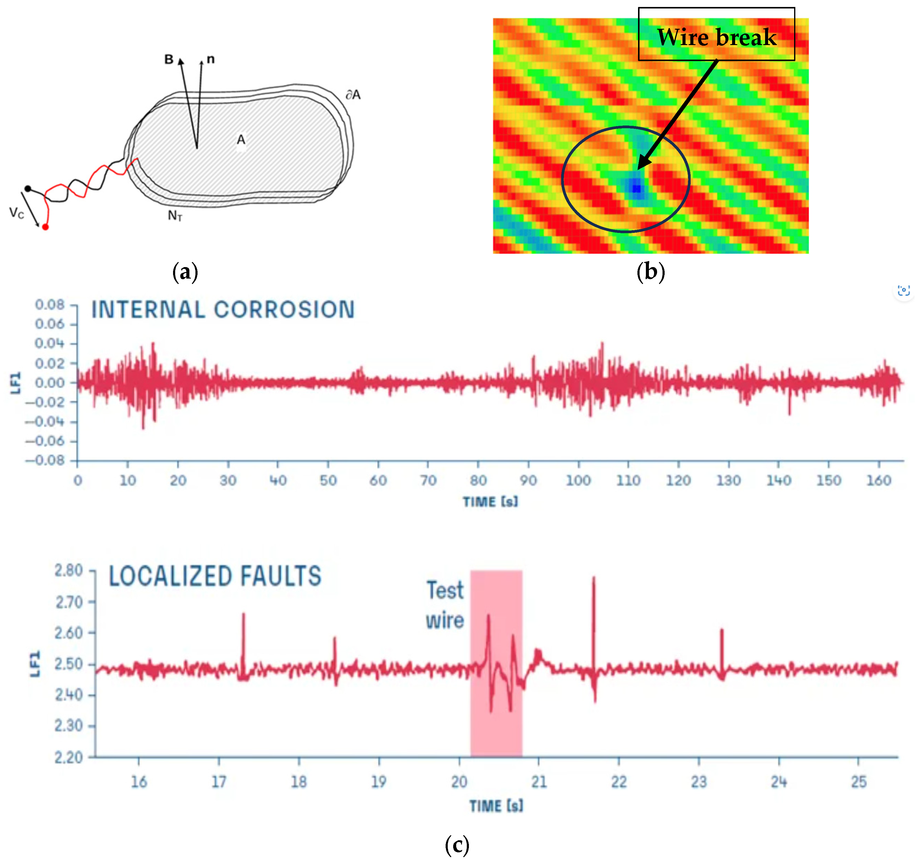
  • Vc is the induced voltage across the coil,
  • Φ is the magnetic flux through the surface A,
  • Lc denotes the inductance of the coil, and di is the electric current flowing through it,
  • B is the magnetic flux density,
  • n is the unit normal vector to the surface,
  • v is the velocity of the conductor.
The output voltage can be derived from Equation (4) for three canonical cases as follows:
V c , i = Φ t = A c d B d t A c B ω A c B v
where
  • Ac is the effective cross-sectional area of the coil,
  • ω is the angular velocity of rotation,
  • ∇B represents the spatial gradient of the magnetic field.
The first case relates to a fixed coil in a time-varying magnetic field. The second case involves a coil rotating at angular speed ω in a constant magnetic field. The third case concerns a coil translating at speed v in a constant field with a gradient.
The dominant component of the induced voltage signal in coils LF1 and LF2 is the first case (Equation (5)), generated mainly by local wire damage (cracks, abrasion, spot corrosion). The second and third cases result from the design features of the measuring head and the lack of peripheral symmetry of the cylindrical coils and the longitudinal symmetry of the distribution of the magnetic field near the rope. The second case reproduces information about the torsional vibrations of the rope and the asymmetry of the arrangement of the rope strands around the circumference. The third case reflects the information about the longitudinal vibrations of the rope, the asymmetry of the strand pitch, and the influence of changes in the speed of the rope scanning on the position of the magnetic plane of the neutral measuring head. The signal from a coreless coil is described by Equation (6).
V c = d Φ d t = A c d B d t + A c B ω + A c B v
The frequency characteristics of the coil—a series circuit R c L c —are described by the impedance expressed by Formula (7) and the goodness of the coil described by Formula (8). The time constant τ of the coil without the influence of the winding capacitance is given by Formula (9), and the change in voltage and current in transients is described by Formulas (10) and (11) :
Z c ω s = Z c ω s e j φ ω s = R ω s + j X ω s = R c + j ω s L c j 1 ω s C c
Q = X L R
τ = R c L c
u t = I · R c + L c d i t d t = V · e τ · t
i t = V R 1 e τ · t
where
  • e is the base of the Natural Logarithm = 2.71828,
  • R = R c is the actual part of the coil impedance,
  • X = X L X c is the imaginary part of the coil impedance (reactance),
  • X L = ω s L c is the inductive reactance of the coil,
  • X C = 1 / ω s C c is the capacitive reactance of the coil related to the winding-to-turn capacitance,
  • ω s = 2 π f s is the circular frequency of a signal (magnetic field) with a frequency of  f s ,
  • Z c = R 2 + X 2 is an impedance module,
  • φ is the phase angle between the voltage and electric current.
The study used a GP-type measuring head developed at the AGH University of Science and Technology, in which the LF1 and LF2 coils are series N L F 1 circuits and cylindrical coils evenly distributed around the circumference and N L F 2 wound on an E-type ferromagnetic core in order to
  • Reduce inter-turn capacitances,
  • Increase the inductance of the coil and the amplitude of the induced voltage, μ = μ m μ 0 ,
  • Differentiate the induced signal on the basis of known core design features.
The LF1 and LF2 signals recorded in the defectograph reproduce the resultant signals of the cylindrical coils, taking into account the following:
  • Coil nonlinearity resulting from the influence of the magnetization characteristics of the ferromagnetic core B H on the instantaneous values of current i t in the coil winding and hysteresis and eddy current losses in the core. For low-magnetic-field frequencies, the unit power of the losses P F e , h in the ferromagnetic and hysteresis cores is proportional to the frequency (12), and the unit power of eddy current losses P e c is proportional to the square of the frequency (13);
  • Local heterogeneity of the magnetic permeability of rope wires (influence of different degrees of their degradation and current material strain, abrasion, and cracking of wires);
  • Actual characteristics of the point sensitivity of the LF1 and LF2 coils, taking into account the heterogeneity of their sensitivity along the circuit, depending on the number of cylindrical coils distributed along the circuit on a given radius and the parameters of the magnetic field concentrator;
  • E-core parameters;
  • The impact of transmission line parameters;
  • Parameters of the defectograph input circuit;
  • The impact of the scanning speed compensation system;
  • Continuous quantization parameters in Analog-to-Digital convectors (ADCs).
    P F e , h = σ h · f · B m n
    P e c = σ e c · f 2 · B m 2
where
  • σ h is the coefficient depending on the grade of core material;
  • σ w is the coefficient depending on the grade of core material, its geometry and construction;
  • f is the frequency;
  • B m is the amplitude of magnetic induction in the core;
  • n is the power exponent equal to 1.6 for B m 0,1   T ; 1,0   T and 2.0 for   B m 1,0   T ; 1,6   T .
The nonlinearity of the LF1 and LF2 coils means that the fundamental frequencies of the source of the local magnetic anomaly and their harmonics and the frequencies of the modulation products are expected in the signal spectrum. As the density of defects in the rope increases, the spectrum will be further modified by the effect of averaging the spectra of individual defects, considering the distance between defects. Discrete signals L F 1 k and signals L F 2 k recorded in the flaw detector are described by the signal model (Equation (14)):
L F i k = s i g n a l L F i k + n o i s e L F i k
where
  • k is the discrete time;
  • s i g n a l L F i is the voltage component at the coil output generated by the technical condition of the wire rope L F i ;
  • n o i s e L F i is the voltage component at the coil output generated by other sources of magnetic field heterogeneity L F i .
A measurement head equipped with two LF sensing coils LF1 and LF2, positioned at different radii R1 and R2, enables quantitative analysis of rope defects (anomaly sources) and localization of their position relative to the axis of the measurement head. This process takes into account a magnetic anomaly model, the amplitudes of the magnetic anomalies recorded in the LF1 and LF2 channels, and calibration data from the measurement system, as described by Equations (15) and (16) [38].
r R = k · A 1 A 2 1 / m 1 k A 2 A 1 1 / m
A 0 = A 1 · r m
where
r = R 1 r is the distance from the anomaly source to the inner sensing coil LF1; R = R 2 R 1 is the fundamental signal that depends only on the flaw parameters and is independent of the flaw location and the geometry of the search coils;
A 1 = k 1 A 0 R 1 r m is the amplitude of the magnetic anomaly recorded by the LF1 coil;
A 2 = k 2 A 0 R 2 r m is the amplitude of the magnetic anomaly recorded by the LF2 coil.
Reliable detection of rope defects and meeting the criterion of defect symptoms according to EN 12927:2019 requires minimizing the noise level, including the following components:
  • Signal harmonics that reproduce the structural features of the rope and the measuring head, and in the current data analysis algorithms, MRT methods are considered structural noise;
  • Color noise being the resultant of quantization noise, thermal noise of the measurement path, and external low-frequency electromagnetic interference.
For this purpose, various non-standardized algorithms for the analysis of MRT measurement data in the time, frequency, rope scanning distance, order, and modulation domains are used around the world [39,40,41,42], which, together with the design features of the measuring head, often constitute the manufacturer’s know-how. As a result, the user of the MRT test track is not able to fully use the diagnostic potential of the existing testing equipment and software and optimally adapt the diagnostic criteria to new types of steel ropes, especially polymer-impregnated steel ropes. Such a situation is one of the premises for the occurrence of type II errors in MRT diagnoses and occasional cases of emergencies due to breaking of steel ropes.
The spectral complexity of the LF1 and LF2 signals makes these signals preferable for numerical synchronization of data from periodic technical inspections of the rope, which will ensure the objective comparison of test results recommended by the ISO 4309 standard and minimize the impact of the human factor on the probability of diagnosis. One of the possible methods for the automatic synchronization of time series with a similar spectrum is the DTW algorithm—Dynamic Time Warping.

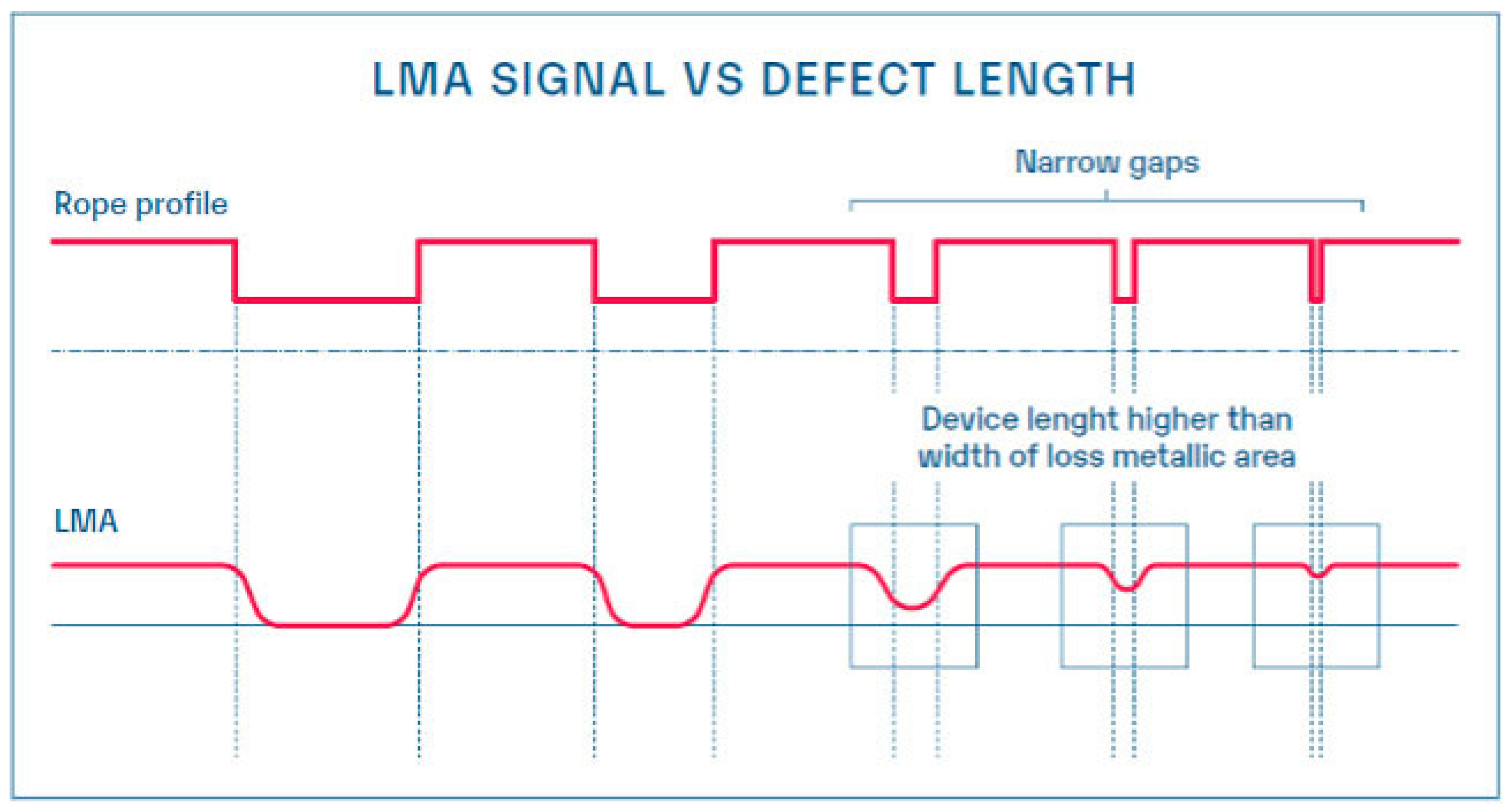
2.1.2. Numerical Model of the LMA Signal

The LMA (Loss of Metallic Area) signal generated by Hall sensors has been used to indirectly detect changes in the average magnetic properties of the rope fragment material, including magnetic permeability [43], coercivity, and remanence μ m H c B r . Changes in the magnetic properties of the rope material can be caused by, among others, the current state of stress, change in the diameter of the rope, local plastic deformation of the wires or the rope, corrosion of the wires, fatigue of the material, and changes in the temperature of the material [44]. A higher number of broken or corroded wires corresponds to a greater reluctance of the tested rope fragment. In the MRT method, the Hall sensor can be mounted as follows:
  • In the air gap under the pole piece of the magnetization circuit in order to record the induction of the magnetizing field F of the rope   B m . With the known parameters of the magnetizing circuit (geometry, magnetomotive force, and magnetic flux Φ m ), the signal indirectly reflects the magnetic reluctance R = F / Φ m l / μ m · S w r S w r of a fragment of the tested rope with a cross-section of the ferromagnetic part (the rope fragment is a component of the main magnetic circuit) and the existing state of magnetization of the rope.
  • Inside the measuring head, in which the rope is fully demagnetized B m , B m , in order to record the scattered magnetic field inside the head Φ i n , depending on the existing magnetization of the rope, the magnetic parameters prevailing in the air gaps of both pole pieces of the measuring head, local magnetic anomalies of the rope, and broadband Barkhausen noise.
  • Outside near the probe in order to record the external scattered magnetic field Φ o u t of the probe and the level of magnetization of the rope when magnetizing the rope along the “original” magnetization curve, taking into account the position of the Hall sensors relative to the external magnetic neutral axis.
In contrast to the coils’ Hall effect, sensors can measure magnetic field strength in a static mode, as they are based on the Lorentz force acting across the sensor (Figure 5).
The response of a Hall effect sensor is given by the formula in Equation (17) up to the point of saturation determined by the constraints of the power supply:
V H = R H i · B s
where
  • V H 
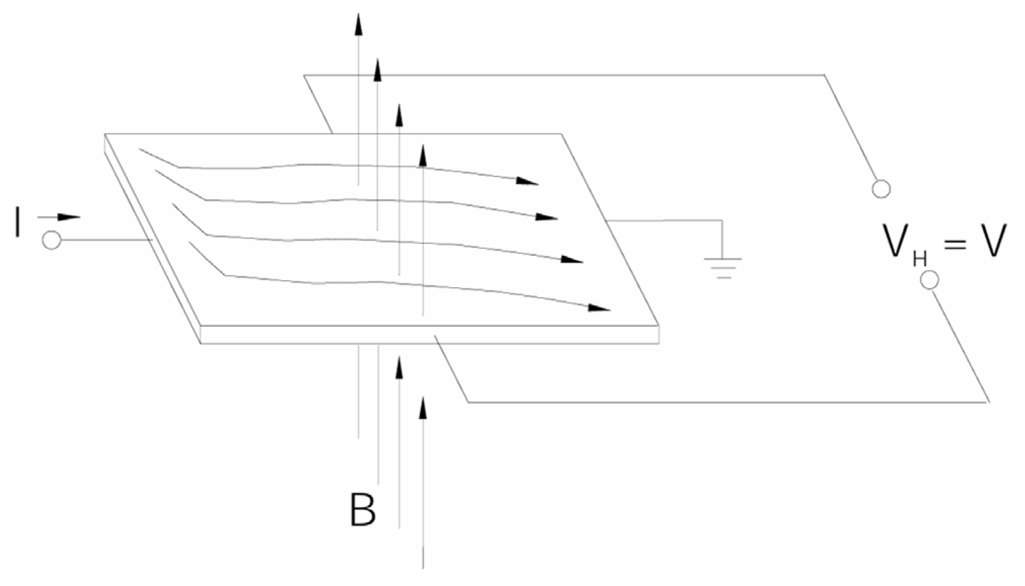
is the output voltage of the Hall sensor;
  • R H is the resistance of the Hall sensor;
  • i is the electric current;
  • s is the thickness of the conductor;
  • B is the magnetic flux density (the only changing parameter in the input).
Hall sensors have many advantages, including being cheap, small, and having the ability to detect both the presence and direction of a magnetic field at a given point in space. They are highly resistant to dust, dirt, and moisture, making them ideal for use in harsh environmental conditions and in typical MRT conditions. Fast response times allow them to be used effectively in dynamic applications. Hall effect sensors are available with different sensitivities, which facilitates their proper selection at the stage of designing the measuring head for a given range of wire rope diameters. The signals of several Hall effect sensors evenly arranged around the rope can be converted to a conventional 2D curve that shows the same typical defect signals as the search coil (Figure 6). The approximate relationship between the LF signal and the LMA is described in Formula (18). The measuring head for testing wire ropes with multiple Hall sensors instead of search coils was developed at the end of the twentieth century at the Technical University of Stuttgart and is known as the “STUTTGART High Resolution Magnetic Rope Testing Method” [46].
V H t d t = R H i s · d B t d t V L F t
The existing differences between the signal from the search coil and the derivative of the signal from the Hall sensor result from the size of the cross-sectional area of the magnetosensitive element in which the measurement of the surrounding magnetic field is performed (it is larger for the coil) and the nonlinearity introduced by the ferromagnetic core of the coil. Using these methods, it is possible to access more information about a defect from the shape of the magnetic field:
  • The location around the rope circumference (e.g., upper or lower side of a track rope),
  • The shape of the defect,
  • The arrangement of clusters of wire breaks,
  • The depth within the rope (for stranded ropes) and the distribution of wire breaks, e.g., in a single strand.
The theoretical signature of the magnetic anomaly from a broken single wire of a wire rope is described by the dipole model and the Nussbaum formulas in Equations (19) and (20). The actual magnetic signature of rope defects changes as the damage density and rope type increase. The signatures of the internal defects of the rope are weakened in multi-layer polymer-impregnated steel ropes, which results from the lack of mechanical contact of individual layers of the strands.
B a x i a l z n = I · π d 2 16 π · k B z k · 2 · z k z n 2 a 2 z k z n 2 + a 2 5 / 2
B r a d i a l z n = I · cos α · π d 2 16 π · k B z k · 3 · z k z n · a z k z n 2 + a 2 5 / 2
where
  • B a x i a l is the axial component of magnetic flux density of the defect field;
  • B r a d i a l is the radial component of magnetic flux density of the defect field;
  • a is the distance from a measuring point on the surface to the rope axis;
  • d is the wire diameter;
  • I is the current;
  • z k ,   z n is the longitudinal coordinate in relation to the wire break end;
  • α is the angle;
  • B is the difference in flux density.
In addition to their advantages, Hall sensors also have some weaknesses. Temperature fluctuations can affect their accuracy, so they require the implementation of temperature compensation mechanisms. Precise calibration is often crucial to guarantee accurate magnetic field measurements. Hall sensors typically exhibit higher noise and lower sensitivity compared with other magnetic field sensors, and they require a current-stabilized power supply to operate. The current consumption of a Hall effect sensor is much higher than that of magnetoresistive (AMR, GMR, TMR) and magnetoimpedance (MI) sensors. The LMA signal is much more sensitive to the external environment (electromagnetic interference, moving ferromagnetic objects) than the LF signal of the search coil. Before the MRT results are graphically displayed, the LMA signal is usually highly filtered by software procedures that can significantly alter it (Figure 7). If the defect area is longer than the distance between the pole pieces of the measuring head, then the reduction in the volume and cross-section of the rope are proportional—the LMA signal correctly reproduces the LMV volume changes in the metallic part of the steel rope not impregnated with polymer. If the fault is shorter than the pole piece spacing, the LMA signal has a lower amplitude than expected and does not correctly reproduce the volumetric changes in the metallic part. In the case of polymer-impregnated steel rope, the LMA signal will also change as the gap between successive layers of strands changes. A filtered LMA signal provides better trend tracking and interpretation, but the end user should remain in control of all processes. The use of closed algorithms over which the client has no control can be dangerous and is a prerequisite for the occurrence of type I and II errors in the diagnosis from MRT examinations.
The LMA discrete signal model is described by Equation (21):
L M A k = s i g n a l L M A k + n o i s e L M A k
where
  • k is discrete time;
  • s i g n a l L M A is the LMA voltage component at the output of the Hall sensor generated by the technical condition of the wire rope;
  • n o i s e L M A is the LMA voltage component at the output of the Hall sensor generated by other sources of magnetic field heterogeneity.
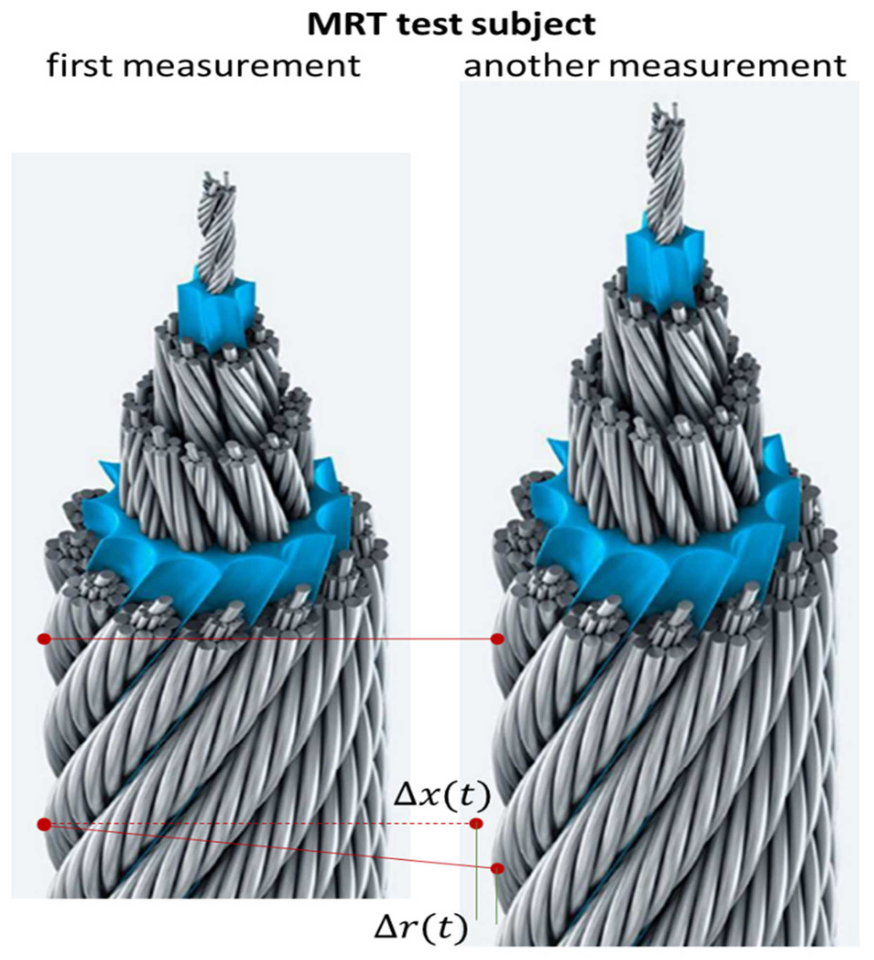
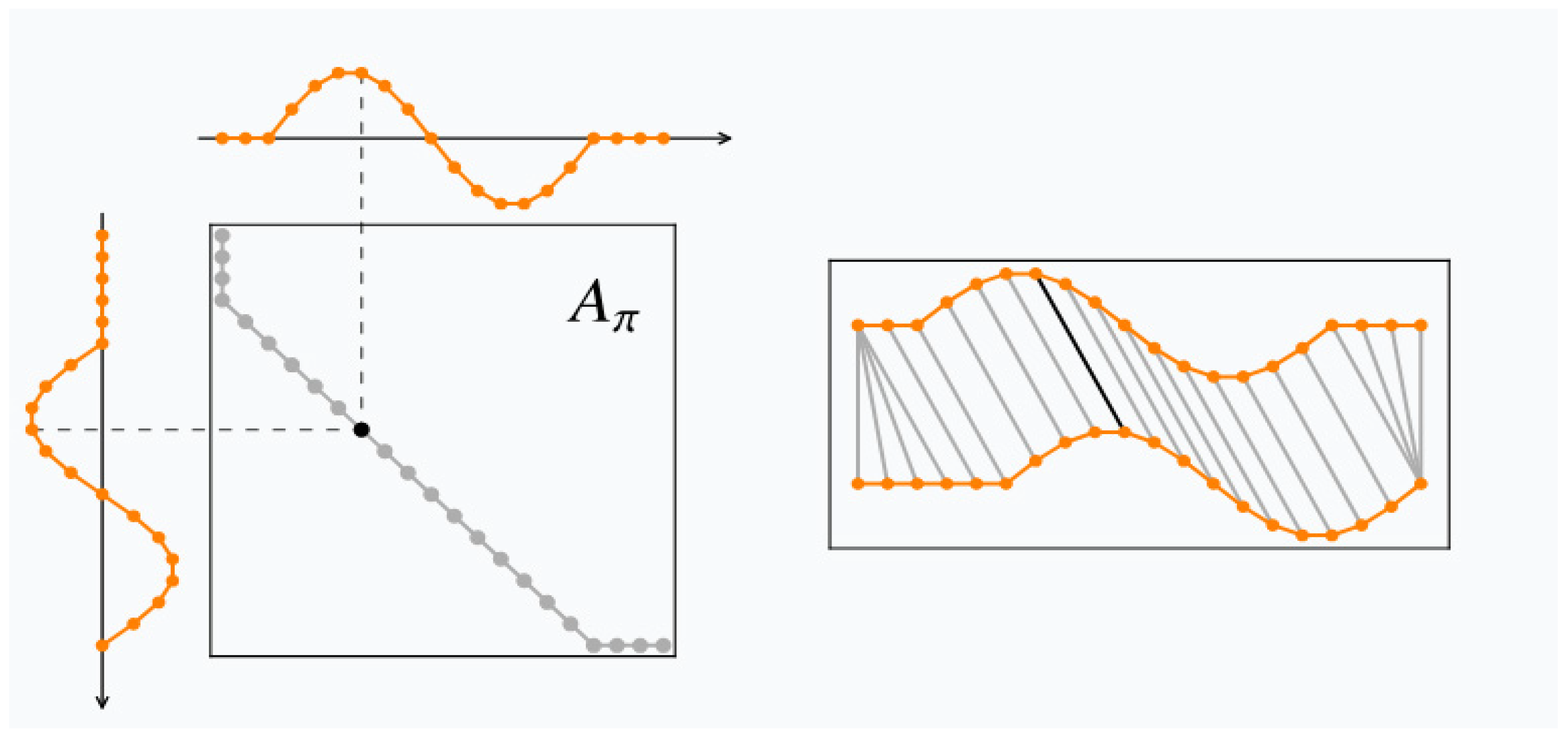
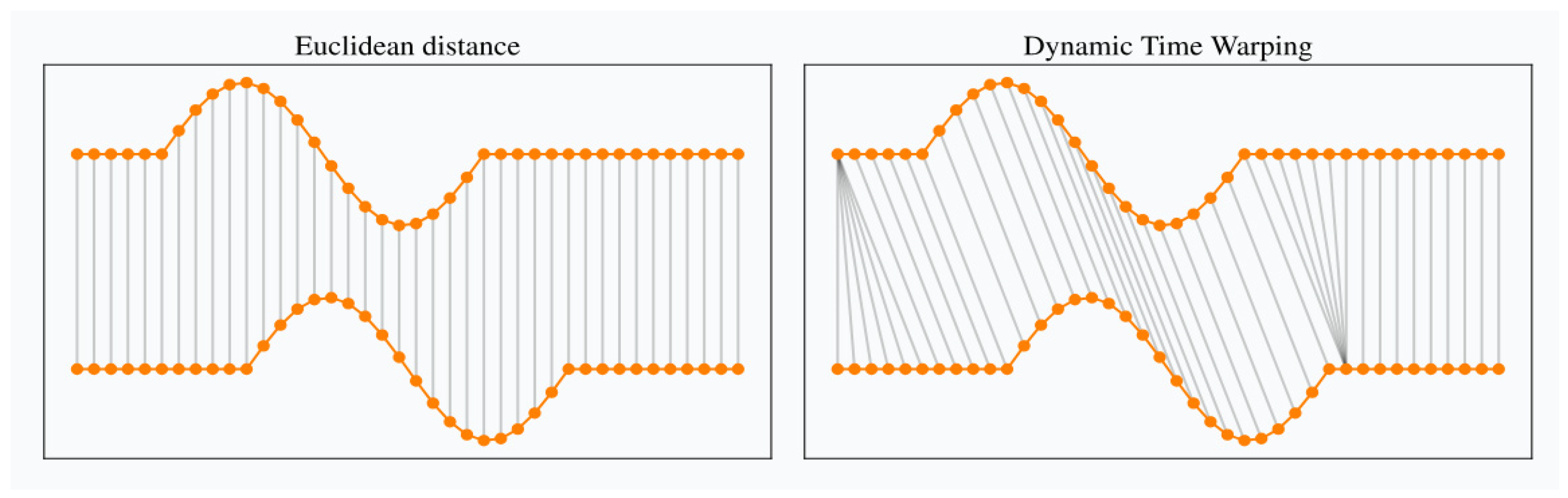
The reliable detection of rope defects and meeting the defect symptom criterion according to EN 12927:2019 requires minimizing the noise level. The small number of Hall sensors used in the GP head, the averaging of the measured magnetic field information, and temperature drift make the LMA signal less suitable than the LF signal for synchronizing data from periodic MRT inspections of the rope, especially in the phase preceding the appearance of wire breakage or developed internal corrosion of compact ropes.
Despite the advantages of a multi-sensor probe head, including the ability to obtain measurement results in the form of a magnetogram, the majority of MRT users worldwide use a single Hall sensor measurement path. In the GP head used in Poland, only two Hall sensors are used, located on the same radius as 180 degrees, which measure the average scattered magnetic field inside the magnetic circuit (measuring head, rope fragment, air gaps between the rope and the pole pieces of the magnetizing circuit based on permanent magnets). The LMA signal recorded in the MD121 flaw detector is a low-resolution low-band filtered signal, which excludes its use for time-series synchronization from periodic non-destructive testing.

2.2. Algorithm DTW

Time-series synchronization can provide a better understanding of the interaction mechanisms between two different signals or systems [49]. Synchronization analysis between spatially separated features is a fundamental procedure in visual pattern recognition [50]. The goal of synchronization measurement and analysis is to characterize the relationship between two systems (e.g., current and reference), which may be identical, non-identical, or different. As coupling strength increases, systems may experience phase synchronization (PS), generalized synchronization (GS), lag synchronization (LS), or complete synchronization (CS) [51].
Synchronization is most often estimated using coherence and spectral properties of the signals. However, this approach is not suitable for characterizing signals that are non-stationary and is limited to capturing linear dependencies between time series.
Because of the analysis of the MRT method, it was found that the synchronization of time series from periodic MRT tests of wire ropes should be carried out based on LF1 and LF2 signals from search coils, which for each channel represent the MISO (Multi-Input, Single-Output) class system. Elongation of the wire rope (structural, operational, final degradation phase) changes the position of the points mapping the same fragment of the rope in the LF signal on the horizontal axis, both in the TIMER and ENCODER modes (Figure 8).
As a result, during rope operation, the spectral content of the harmonic components in the LF1 and LF2 signals, as well as the colored noise ε(k), changes. However, the following remain constant:
  • The proportions between characteristic frequencies resulting from the rope’s pitch and its structural features (such as the number of outer, inner, and core strands);
  • The main component of the colored noise, which reflects dynamic phenomena in the rope system, the noise of the measurement channel, and the level of electromagnetic interference near the measurement head.
L F i r e f k = j a j k · sin ω j · k + φ k + ε i k L F i b k = j a j k + a j k · sin ω j ω j · k + φ k + φ k + ε i k + ε i k
where I = 1,2..k is the discrete time of signal recording; ω = 2πf is the angular frequency of the harmonic signal component; φk is the initial phase of the signal; Δεi is the change in noise characteristics relative to the reference signal.
The spectral features of the above signals, including information about the type of colored noise, are described by power spectral density (PSD) functions, which are normalized to a constant frequency interval width, most commonly, 1 Hz. The power spectral density is denoted by S(f) and is given by
S f = lim f   0 X f 2 f
For a discrete time signal x n   , there is a relationship between the power spectral density S x f and autocorrelation function R x m , which can be given as follows:
S x e i 2 π f   m = + R x m e i 2 π f m
For long ropes, e.g., those used in a mining hoisting machine, the total elongation of the wire rope may exceed many times the pitch of the rope, and the phase shift of the current signal L F b relative to the reference signal L F r e f (e.g., the first recording) will increase with the length of the rope scan. The first step in the synchronization of measurement data should be the automatic determination of the initial offset of the next MRT recording in the extreme position of the rope system, e.g., in the upper or lower skip position, because the rope may be subject to
  • Periodic shortening by the user to equalize the stresses in the multi-rope system and maintain the skip stop parameters at a given level;
  • Automatic shortening under the influence of torsional torsion.
With the change in the length of the rope, its diameter and the pitch of the coiling of the strands in the individual layers of the rope and the distance between the strands change, which leads to an increase in the air gap in the measuring head and a change in the spectrum of the analyzed signal. Significant changes in the spectrum occur especially in the initial phase of operation of polymer-impregnated steel ropes, during the arrangement of strands and the adjustment of the thickness of the polymer layer to the rope-loading parameters. The values of characteristic frequencies related to the structural features of the rope and the characteristics of color noise change. Along with the progressive degradation of the rope (wire breakage, wire abrasion, corrosion, deformation of the rope shape), additional characteristic frequencies and modulation products also appear in the signal spectrum, which change between successive MRT tests. The spectrum also includes characteristic frequencies representing
  • Rope dynamics—transverse and longitudinal vibrations and level of material effort related to the actual operating conditions of the rope system changing between successive MRT tests;
  • Modal properties of the rope, which change under the influence of unknown load history, current loads, temperature, and the technical condition of the rope.
Periodic recording of magnetic anomalies in MRT studies can be performed with different sampling frequencies (TIMER mode, different forward speed of the rope), encoder resolutions (ENCODER mode), and ADC resolution (different flaw detectors). For such a complex problem, it is not possible to use simple methods of time-series synchronization based on the Euclidean distance.
A characteristic feature of MISO systems is the ambiguity of the solution to the opposite problem—the identification of input signals based on the output signal. In the case of MRT studies, this problem is mapped by the probability of diagnosis P O D < 1.0 and must also be considered when testing new algorithms for the analysis of measurement data.
In terms of analysis, the problem of time-series synchronization from MRT studies fits into the classic area of numerical analysis of discrete signals in time with a similar, but not the same, spectrum and initial offset. A common algorithm used for this class of problems is Dynamic Time Wrapping (DTW). DTW can be used to compare sequences with unequal lengths and unsynchronized sequences. DTW is a measure of similarity between two time series that was introduced in the literature by Vintsyuk [52,53] and Sakoe and Chiba [54]. The original use of DTW was speech analysis applications [55]. In addition to speech analysis, DTW is now also widely used in machine learning, medical sciences, econometrics, chemometrics, healthcare, marketing, sports analytics, robotics, epidemiology, and general time series mining, but it is not used in non-destructive testing (NDT) and condition monitoring (SHM) systems of wire ropes. The code of the classic DTW algorithm and examples of its use are currently available in the following software:
  • Matlab [56,57,58,59];
  • C++ [60];
  • R—package dtw described in [61];
  • Python—dtw-python package [62], which is a clone of the dtw package from R. Python also includes the fastdtw [63,64] package (installation: pip install fastdtw), which is time-optimized and, for a window of 10,000 data points, is over 200 times faster than the classic DTW, with no information about the quality of time series fitting.
The Fast DTW algorithm is also available in Java [60,65]. Theoretical foundations along with a mathematical description of DTW and sample codes are included in blogs [66,67].
The DTW algorithm relies on the time alignment of the series to assess their similarity. All objects in the time series x = x 0 ,   x 1 , , x n are in the same space R p .
Two time series will be analyzed for the MRT study, x = L F r e f k and x = L F b k , of appropriate lengths n and m , which are a subset of the recorded measurement data from the rope test. It is assumed that all elements of the time series x and x lie in the same p-dimensional space, while the exact timestamps in which the observations occur are ignored—only their order matters. The optimization problem is described by the formula in Equation (25).
D T W q x , x = min π A x , x i , j π d x i , x j q 1 / q
where
  • π is an alignment path of length K , which is a sequence of pairs of indices K i 0 , j 0 , , i K 1 , j K 1 ;
  • A x , x is the set of all acceptable paths.
For a route to be considered acceptable, it should meet the following conditions.
The beginning (or end) of the time series is matched to each other:
  • π 0 = 0,0 ;
  • π K 1 = n 1 , m 1 .
The sequence monotonically builds up in both i as well as j , and all time-series indexes should appear at least once, which can be saved as follows:
  • i k 1 i k i k 1 + 1 ;
  • j k 1 j k j k 1 + 1 .
DTW paths can be represented by a binary matrix whose non-zero entries correspond to the fit between the time series elements. Such a representation is related to the representation of the sequence of indices used above by Equation (25) and illustrated in Figure 9—non-zero entries in the binary matrix are represented as dots, and an equivalent sequence of matches is created on the right side:
A π i , j = 1         i f   i , j π 0         o t h e r w i s e  
Using matrix notation, dynamic time curvature can be written as minimizing the dot product between matrices:
D T W q x , x = min π A x , x A π , D q x , x 1 / q
where D q x , x stores the distance d x , x under q .
Dynamic time warping seeks a time alignment that minimizes the Euclidean distance between aligned series. To do this, it adjusts the timing of the data points to minimize the difference between the two datasets. DTW can be used to compare sequences of unequal length and unsynchronized sequences, which is an advantage of this algorithm over simple methods, i.e., Euclidean distance, which is effective only if the sequences are of equal length and perfectly aligned. A comparison of the fitting of the series using the Euclidean distance method and DTW is illustrated in Figure 10.
In addition to time-series synchronization, DTW provides more reliable automatic identification of signal characteristics including noisy signals. This is because the aligned time series are very similar, which is a known invariant of Dynamic Time Warping. The shape of the signature of a given signal feature obtained from averaging several time series is not deformed (Figure 11).
DTW is a semi-metric that has the basic properties of metrics:
  • x , x , D T W q x , x 0 ;
  • x , D T W q x , x = 0 .
DTW, however, does not satisfy the triangular inequality and identities of the indistinguishable, but is invariant for time changes and time shifts regardless of their time span. During the time-series analysis, additional constraints can be imposed on the set of allowable paths in order to obtain invariance for only local deformations in a given analysis window and to limit the analyzed set of time deformations, which speeds up the calculation. Such restrictions, e.g., in the form of the Sakoe–Chiba band or the Itakura parallelogram, translate into the enforcement of non-zero entries in the A π to stay close to the diagonal [53,54].
Time series comparison via DTW involves several key steps:
  • Detrending and z-score normalization of the time series—a preprocessing step that addresses DTW’s sensitivity to trend differences. Detrending removes any increasing or decreasing trends in the time series, while z-score normalization scales the values to a mean of zero and a standard deviation of one.
  • Computation of the distance matrix between all pairs of samples—the matrix contains pairwise distances between all combinations of samples in the two time series. Although Euclidean distance works well in many cases, other metrics may be more appropriate, depending on the data.
  • Computation of a cost matrix from the distance matrix—the cost matrix is derived from the distance matrix by recursively accumulating distances from neighbor to neighbor, starting from the initial corner (bottom left) to the final corner (top right). Different neighborhood rules define how these costs are propagated, e.g.,
Orthogonal only: accumulation occurs in x and y directions only, ignoring diagonals.
Orthogonal and diagonal moves: diagonal movements are also considered, typically weighted by a factor of √2 (1.414) to balance with orthogonal steps. The value of each cell in the matrix represents the slope or effort required to pass through it.
Finding the least-cost path within the cost matrix is the step where time warping occurs. The least-cost path minimizes the total cost from start to end of the cost matrix, optimally aligning the two time series.
Computation of a similarity metric based on the least-cost path—the simplest approach is to sum the distances of all points along the path. When comparing time series of different lengths, additional normalization is performed.
Typical options include the following:
(a) Sum of lengths: normalize by the combined length of both time series; (b) automatic distance summation: normalize by the sum of distances between neighboring samples in each series.
Normalized metrics enable comparisons across datasets with varying characteristics.

2.3. Subject of Research

The verification of the possibility of using the DTW algorithm in the extended MRT data analysis was performed as follows:
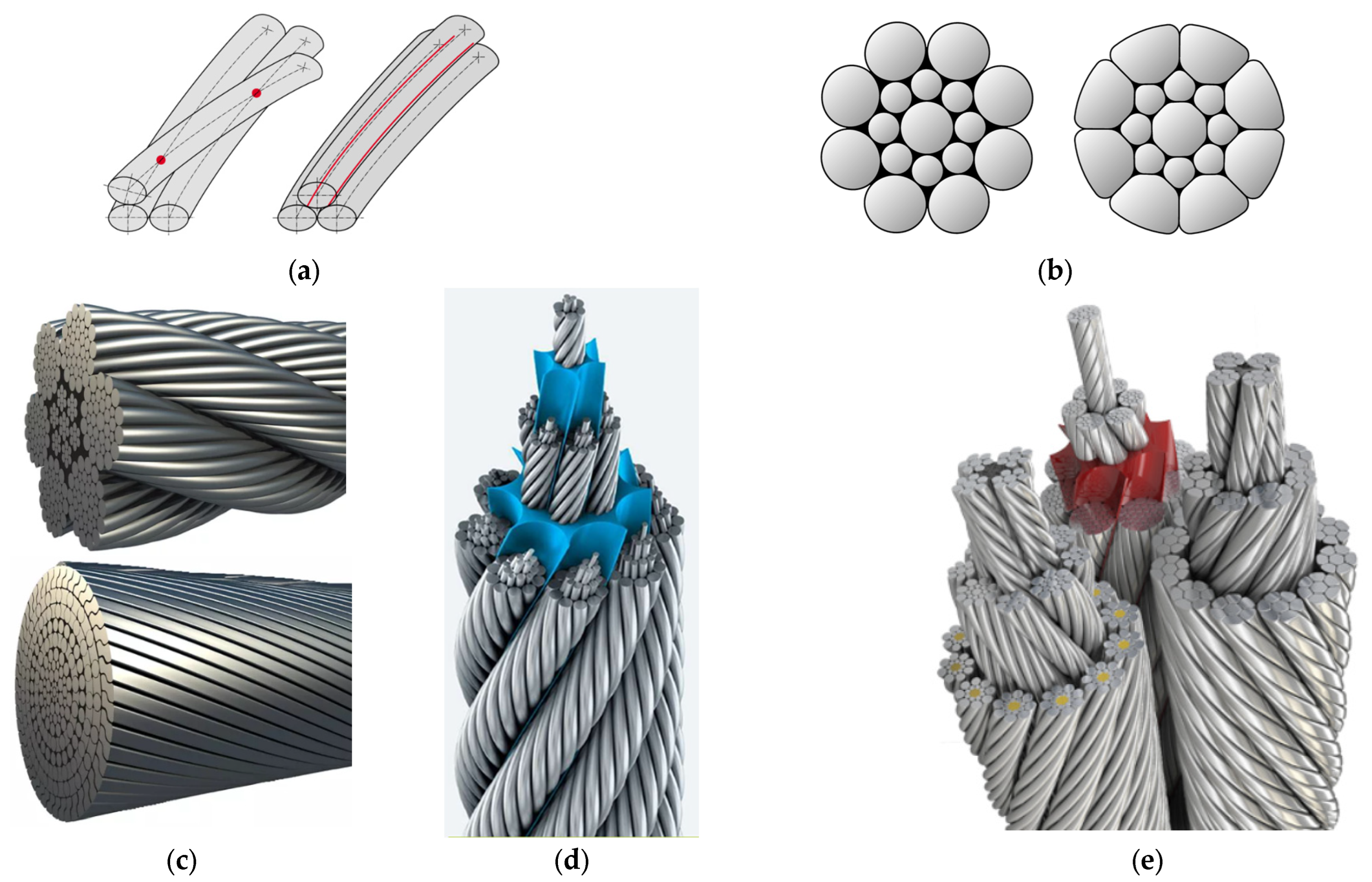
  • During an active experiment in the AGH UST laboratory carried out on a looped (endless) single-layer six-strand Seale 6x19+NF steel rope with a Drumet natural Figure 12a. At the stage of production and braiding, artificial defects in the structure of various types were modeled into the lines and introduced at different depths of the rope cross-section [68]. The rope was located in a dry room and was not exposed to corrosion and fatigue. It was subject to demagnetization during classes with students mastering the technology of MRT testing and verification of new measurement paths and algorithms for steel rope diagnostics. The analyzed measurement data came from a recording in which the rope was not loaded with longitudinal force and was set in translational motion at a set stabilized forward speed through a wheel driven by an electric motor controlled from an inverter. The laboratory stand ensured long-term reproducibility of the diagnostic symptoms of rope damage.
  • During passive experiments based on archival results from periodic tests of the technical condition of steel ropes using the MRT method in the Polish hard coal and copper mining industry, including the following:
  • Two-layer round-strand steel rope 22.0 17x7+Ao Z/s-n-I-N-g-1570-WT-75/TT-2 containing 119 wires in 11 external strands and 6 internal strands on a natural fiber core (Figure 12b), used since 6.12.2004 in the “Guido” shaft of the Coal Mining Museum in Zabrze as a carrying rope for a cage hoist. Rope diameter 22 mm, rope coil stroke 180 mm, total rope length 190 m, safety factor when applied 9.84, min. safety factor 7.5. There is one stable wire break in the rope, which has so far been used for the initial synchronization of time series by the visual method. The symptom of wire breakage was used in the DTW algorithm to optimize the width of the rope fragment analysis window. Characteristics of the mining shaft hoist are as follows: hoisting machine B 1200/AC; hoisting class II; type, felling machine; driving speed 2 m/s; environmental conditions in exhaust shaft, wet; pulling depth, 170 m; number of pulls, approx. 5/week. Corrosion processes dominate in the lines.
(a)
Single-layer wire rope NRHD24 by Arcelor Mittal containing 360 wires in 12 outer strands and 12 Warrington type core strands (Figure 12c). Rope used in a copper mine as an equalization rope is exposed to material fatigue and corrosion of external and core wires in places where the zinc-based protective layer is worn.
(b)
Double-layer steel line impregnated with STRATOPLAST MF 40.0 8x26WS+EPIWRC 1960 B/N(Zn/Al) z/Z (s/S) by CASAR containing wires in 8 outer strands, 6 inner strands, and 3 core strands. The strands are separated from each other by a polymer layer (Figure 12d). A rope mined in a hard coal mine in an exhaust shaft with aggressive shaft waters. Hoisting machine with KOEPA wheel; traveling speed 16 m/s; pulling number, more than 400/day. The line mainly involves fatigue processes in the presence of developing pitting corrosion of the outer wires in places where the protective layer of Bekaert BEZINAL® 3000 has been wiped off. The risk of corrosion of wires of the internal and core strands is very low until the polymer layer is damaged.

3. Results

The input data for the analysis of time-series synchronization using the DTW algorithm consisted of text files exported by the MD121 View software (developed by Zawada NDT) from binary files generated during periodic MRT inspections of steel wire ropes. These files are archived by certified inspectors performing MRT diagnostics.
Extended analysis of the MRT data was carried out using the commercial software DEWESoftX 2024.3 for signal filtering and spectral analysis [69] and the open-source R 4.4.2 environment with the DTW package [60] developed by Toni Giorgino at the Institute of Biophysics (IBF-CNR), Milano. This software is distributed under the terms of the GNU General Public License Version 2, June 1991.

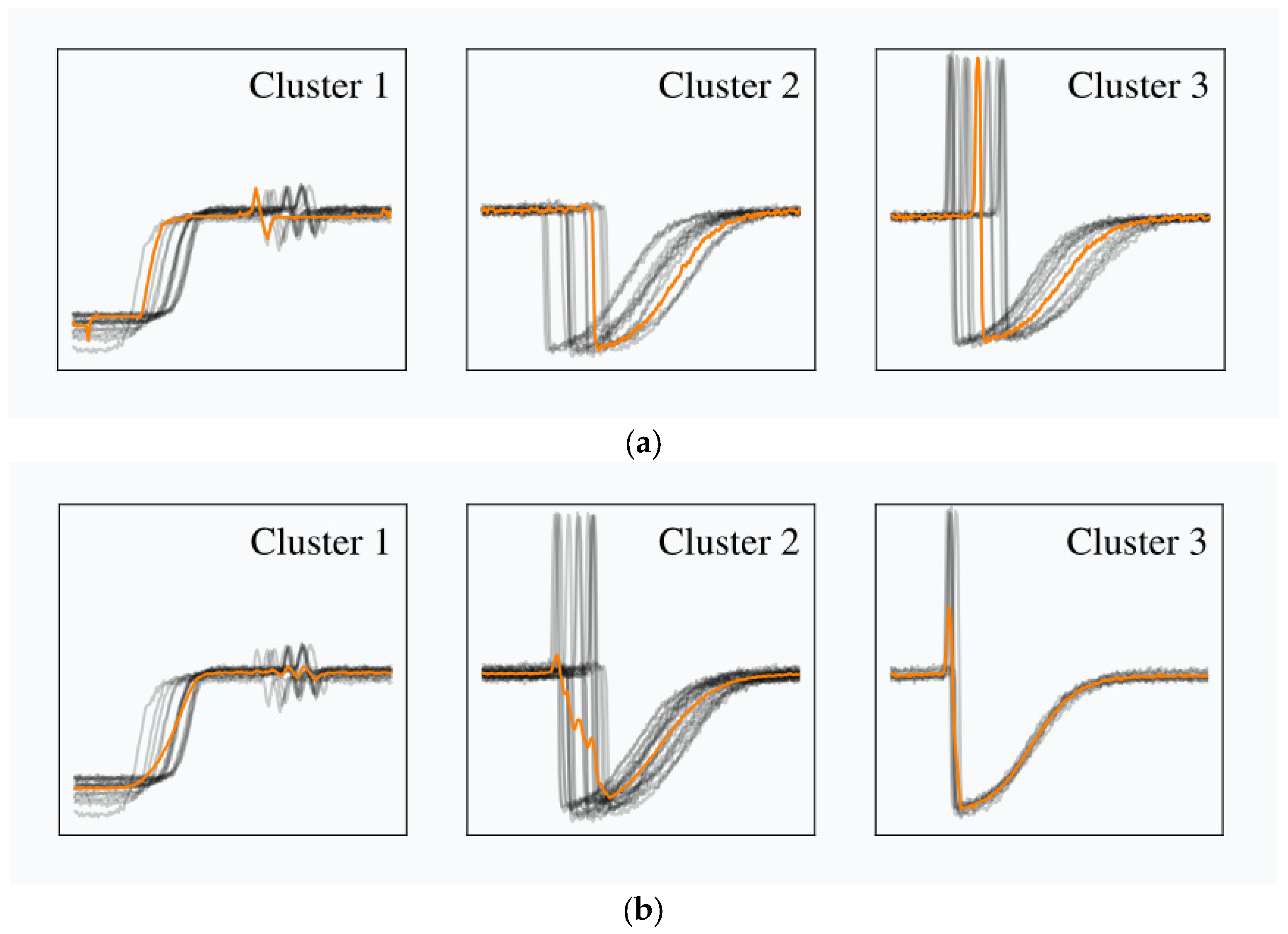
3.1. Active Experiment

The aim of the laboratory tests was to verify the effectiveness and stability of automatic time-series synchronization based on the DTW algorithm using measurement data obtained with different resolutions of scanning ropes with known defects (Figure 13) in ENCODER and TIMER mode. The synchronized segment of the time series was randomly extracted from various parts of the “current” recording, and then, attempts were made to automatically match it to the reference signal with varying initial offsets and sampling frequencies. Examples of the results of the research are illustrated in Figure 13, Figure 14, Figure 15 and Figure 16.
On the basis of the laboratory tests, it was found that the DTW algorithm with additional constraints on the set of acceptable paths correctly synchronized two time series of signals, both in the presence of a strong symptom of a single magnetic anomaly or a group of similar symptoms of magnetic anomalies evenly distributed along the rope, as well as in areas without anomalies of magnetic defects in the rope based on the rope’s structural noise. DTW without local restrictions on the set of permissible paths can generate erroneous synchronization when the analyzed signals are sampled with a significant difference in resolution, and the signal spectrum is dominated by only the fundamental harmonics of the rope construction noise (conducive to the aliasing effect) and weak symptoms of single wire fractures (Figure 16). The risk of mis-synchronization of measurement data can be reduced by considering the results of the synchronization of LF1 and LF2 signals, taking into account the acceptable level of residual signal energy d _ L F i = L F i b L F i r e f   calculated outside the zones of strong magnetic anomalies. An additional criterion for verifying time-series synchronization must also account for the rope’s structural features, determined experimentally, as well as quantitative changes in the PSD spectrum.
The accuracy metrics used were precision (28), recall (29), and the F1 measure (30), which were calculated according to [70]:
P r e c i s i o n = T r u e   P o s i t i v e T r u e   P o s i t i v e + F a l s e   P o s i t i v e
R e c a l l = T r u e   P o s i t i v e T r u e   P o s i t i v e + F a l s e   N e g a t i v e
F 1 m e a s u r e = 2 × P r e c i s i o n × R e c a l l P r e c i s i o n + R e c a l l
where
  • Precision is the ratio of correctly predicted positive observations to the total number of correctly predicted positive observations;
  • Recall is the ratio of correctly predicted positive observations to all observations in the wire rope patterns class;
  • F1 measure is the weighted average of precision and recall.
It was found that DTW can be used to synchronize data recorded in ENCODER mode with different resolutions, np. max. 1.0 mm required by ISO 4309:2017 and 2.5 mm or 5.0 mm used by some MRT users prior to the revision of this standard. It is also possible to synchronize hybrid time series from the measurements in TIMER mode and ENCODER mode, which reduces the risk of misdiagnosis caused by wheel slippage in ENCODER mode and enables the detection of faulty operation of the LF signal compensation system in the flaw detector.
Along with the increase in the difference in the sampling resolution of the signal L F k , the level of residual noise associated with quantization noise and the dynamics of signal changes in magnetic anomaly zones increases, which in the future may be used as a new diagnostic symptom of the MRT method. The residual signal from DTW significantly improves the signal-to-noise ratio—a criterion for objective assessment of the quality of the MRT diagnostic symptom according to EN 12927:2019—and its quantitative and qualitative analysis can be used to verify the correctness of time-series synchronization.
The results of the active experiment confirm the accuracy of the DTW-based time-series synchronization approach under controlled laboratory conditions using known artificial defects, and thus, serve as a preliminary validation of the model.

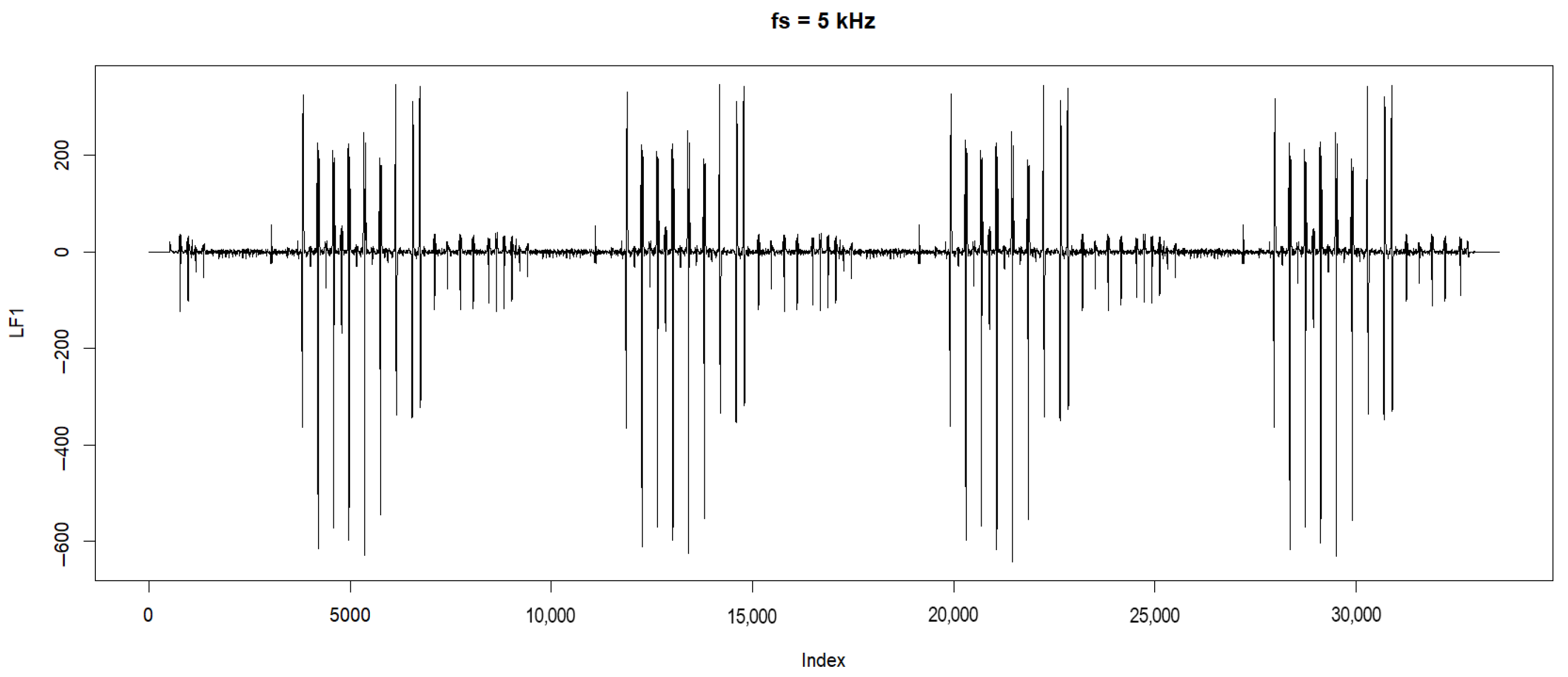
3.2. Passive Experiment

The aim of this stage of the study was as follows:
  • Optimization of the analysis window width is necessary because, for time series x and x’ of length m and n, respectively, and the same ordering, there exist O 3 + 2 2 n n different paths in A x , x , which exponentially increases the required memory and data processing time. The length of the ropes tested in actual industrial installations was many times greater than that of the rope used in the active experiment, and due to the available computational power and data processing time, it was necessary to perform DTW analysis on successive segments of the current recording, taking into account the previous alignment results with the reference data.
  • Verification of the effectiveness of the DTW algorithm in industrial conditions of MRT testing considering that the dynamics of rope operation and its degradation processes are impossible to reproduce in laboratory conditions.
To reduce the time required for initial synchronization of the measurement data, only time series recorded in the same rope movement direction were analyzed. The initial offset resulted from the starting position of the transport vessel (upper skip), the periodic manual shortening of the rope by the user, and the natural elongation/shortening of the rope during operation due to load differences and progressive fatigue degradation of the rope material. The maximum offset between the analyzed time series occurred at the final position of the hoisting vessel.
Automatic recognition of the two rope scanning directions and synchronization of such time series will be developed in future research.
  • The research included data from long-term monitoring of wire ropes of various types and two resolutions of rope scanning in the ENCODER mode:
  • Not less than 1.0 mm, required by ISO 4309:2017;
  • Either 2.5 mm or 5.0 mm, used until the introduction of the amendment to the above-mentioned standard in 2017, and the MRT method still found in some users.
Examples of research results are illustrated in Figure 17, Figure 18, Figure 19, Figure 20, Figure 21 and Figure 22.
Based on the analysis of MRT data from 2020 to 2024 for an over 170-m round-strand steel rope from the Guido shaft, the following was shown (Figure 17 and Figure 18):
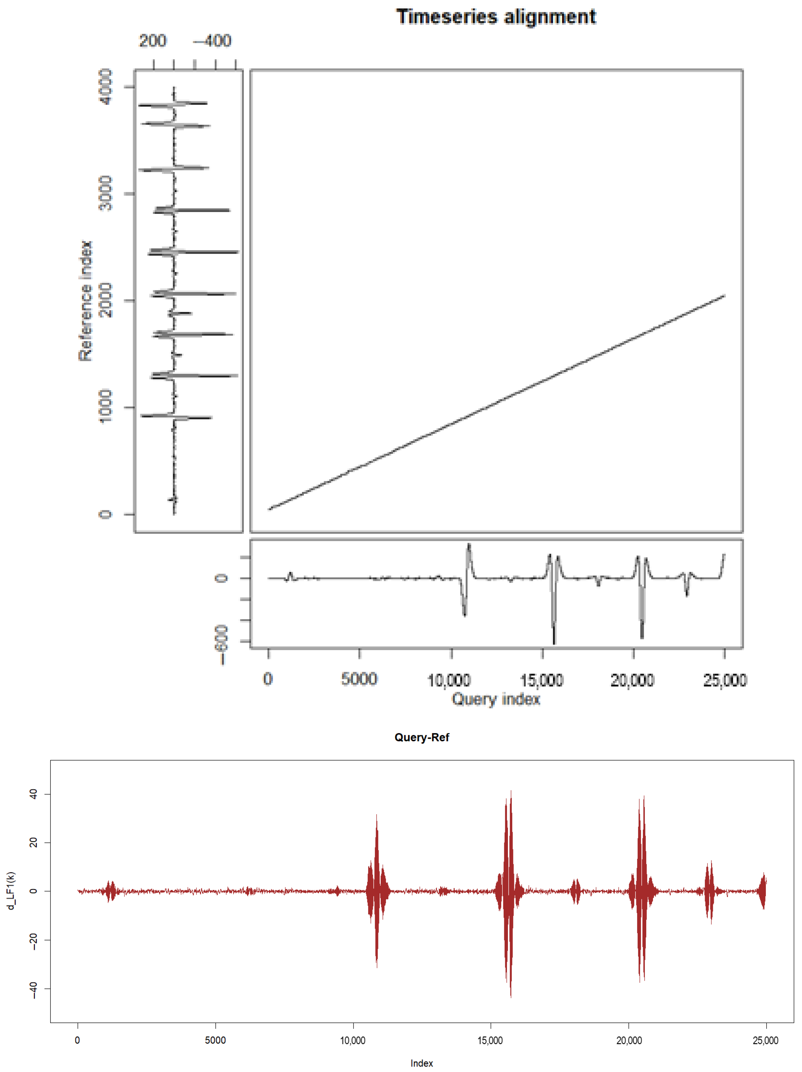
  • The possibility of realizing LF time series matching using the Euclidean distance method in a window not exceeding 1.5 m of rope length and the DTW algorithm in a window of about 9 m;
  • The need to perform DTW analysis with the use of a movable window (similar to the fast Fourier transform, SFFT) due to the limitation of the required memory volume needed to store the calculation results and the calculation time of a single rope fragment;
  • Repeatability of the results of time-series synchronization obtained with the DTW algorithm for LF1 and LF2 signals, with a slight offset between the synchronized LF1 and LF2 signals increasing with the rope’s lifetime, probably resulting from the design features of the GP heads and differences in the magnetic field spectrum on the two rays of the search coils;
  • The ability to monitor progressive corrosion of wires before reaching the ignition criterion of the current diagnostic rule and with a small impact of cyclic material fatigue (lack of broken wires) and abrasions;
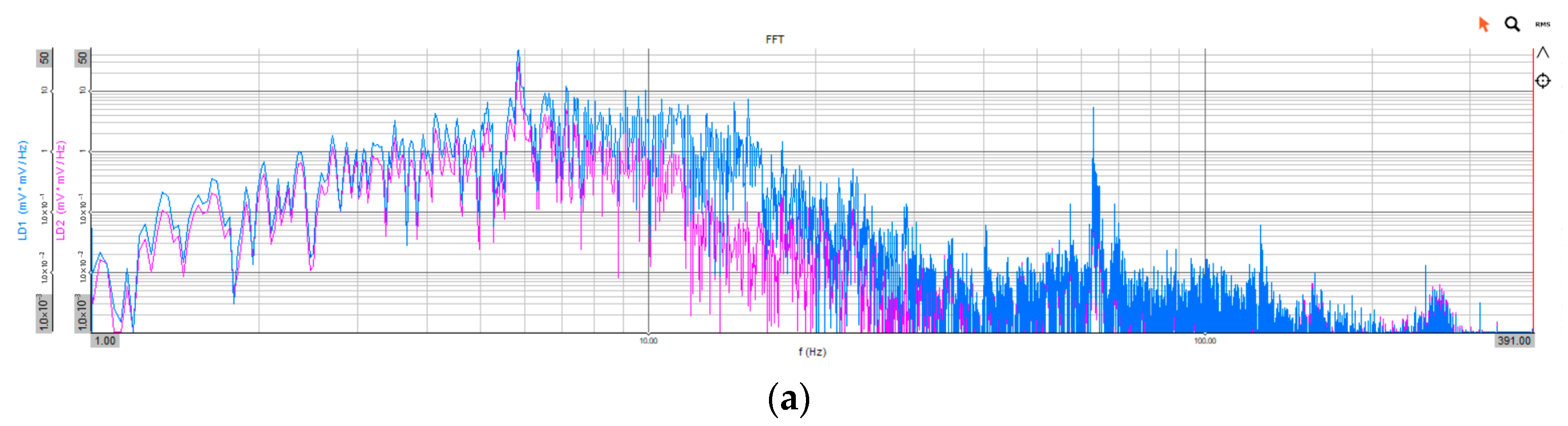
  • The desirability of analyzing harmonic components and noise in the LF signal in the aspect of rope system diagnostics, including longitudinal and transverse vibrations of the rope. After many years of operation, the rope shows repeatability of the frequency of harmonic signals, reflecting the rope’s pitch and the distance between the strands, which are amplitude-modulated along the tested rope—the influence of longitudinal, transverse, and torsional vibrations of the rope.
Based on the analysis of MRT data from 2019 to 2023 for over 680 m NRHD24 steel wire ropes from the copper mine shaft, the effectiveness of LF1 and LF2 time-series synchronization was confirmed for ropes with a multi-strand Warrington steel core despite observed changes in signal characteristics between subsequent experiments. Upon analyzing the signals, distinct differences are observed in the following:
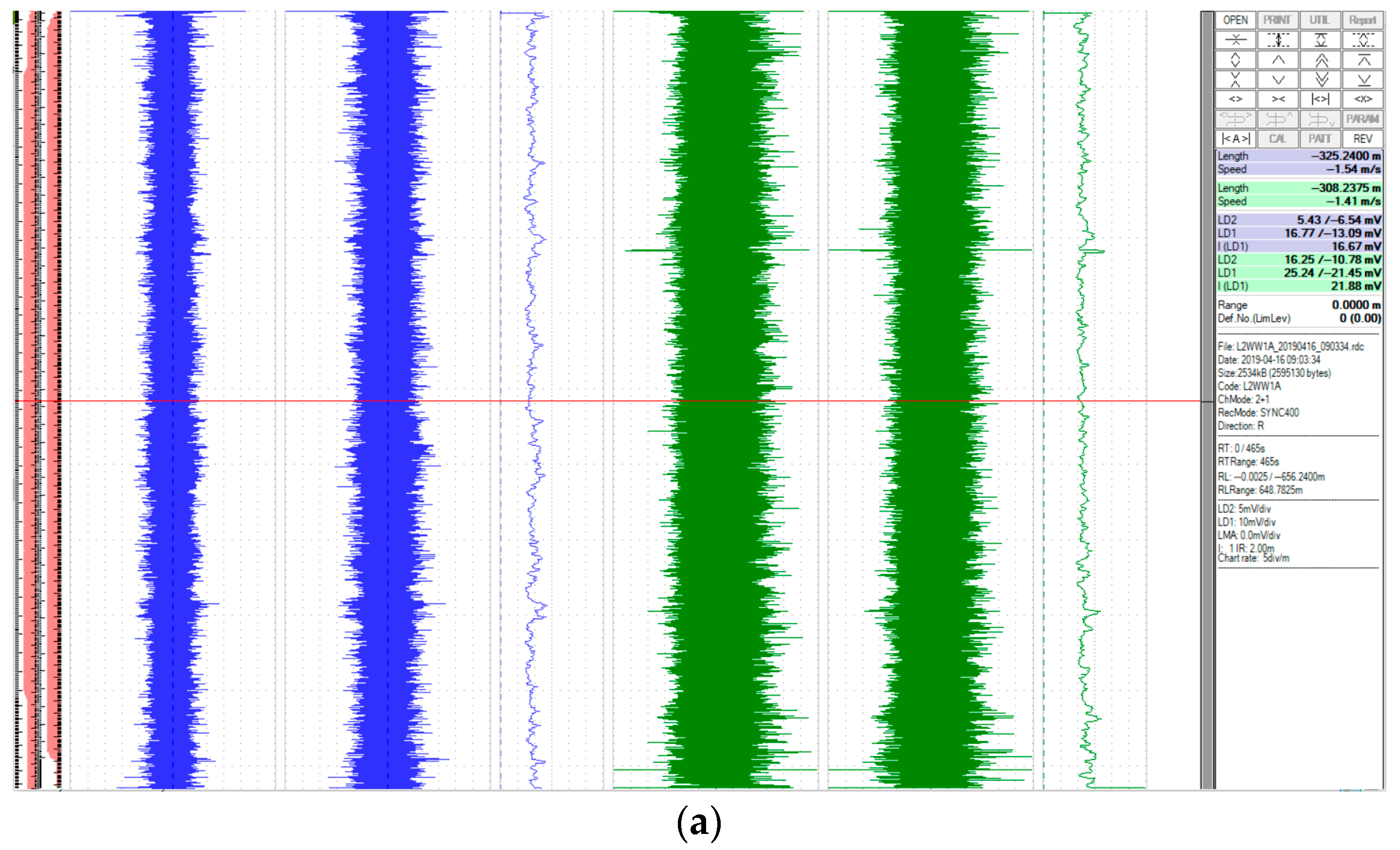
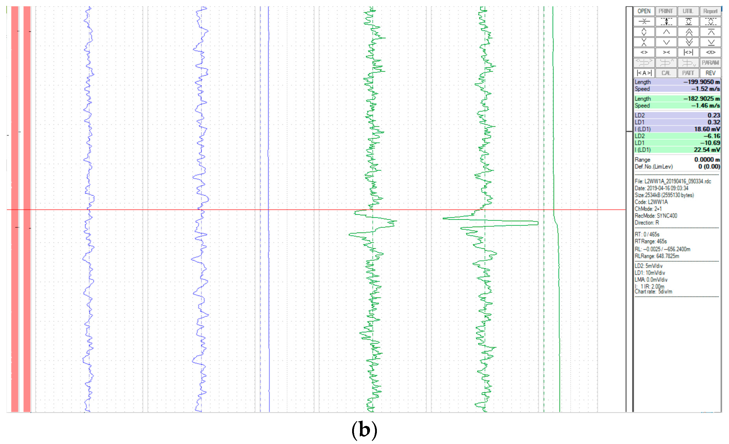
  • The spectrum of the signal that can be visually seen in the time series imaged in the MD121 View software (Figure 19);
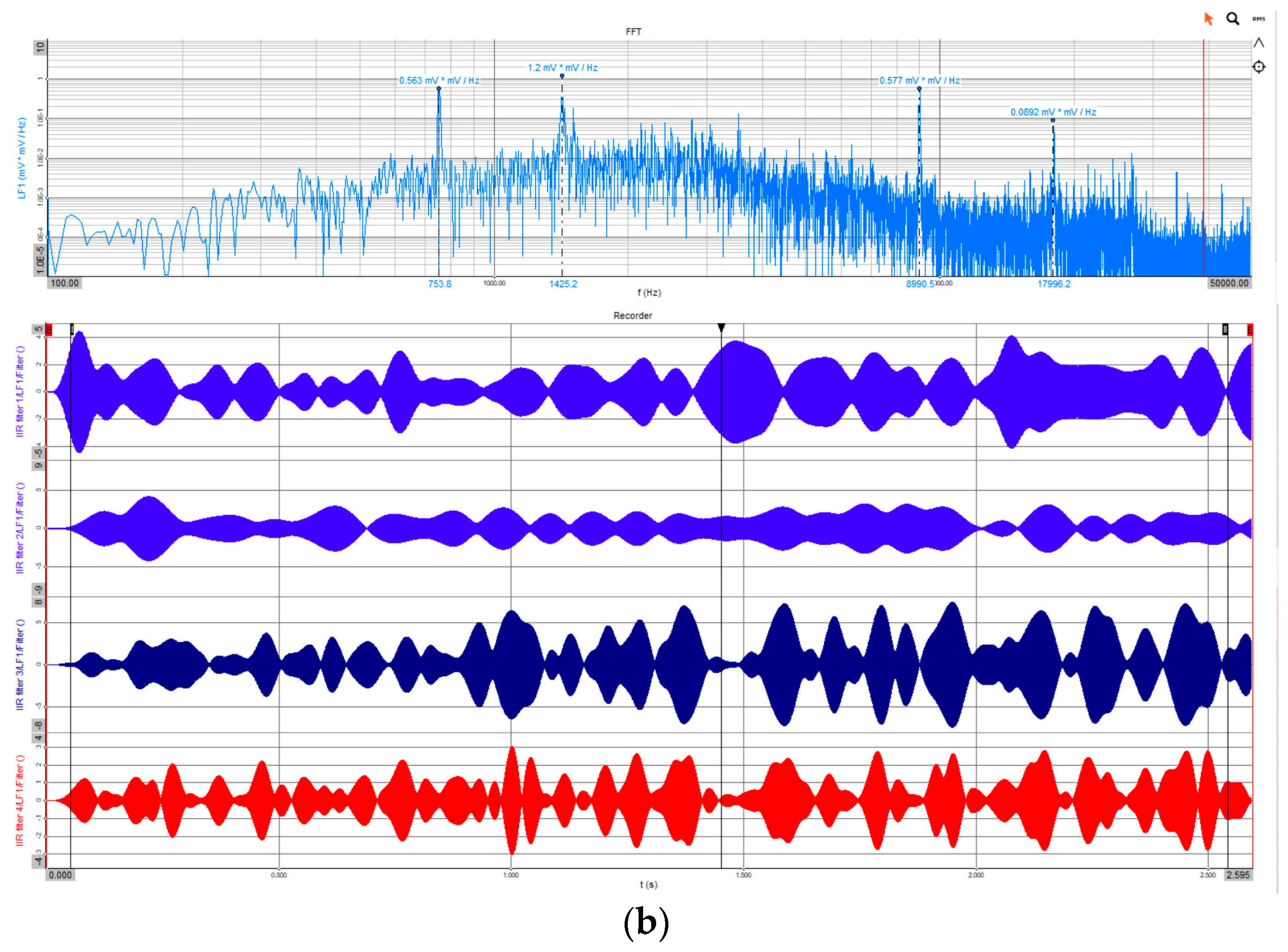
  • Color noise, which increases in the subsequent years of operation of the NRHD24 rope as opposed to the noise of the round-strand rope (Figure 20);
  • Amplitude modulation parameters of harmonic components of signals (Figure 20).
In the residual DTW signal, the following symptoms occur: a broken single wire per 183 m of rope, increasing corrosion of the wires, and processes of cyclic fatigue of the material (Figure 21).
A characteristic feature of the operation of polymer-impregnated steel ropes, e.g., STRATOPLAST MF, is the extended time of strand laying and the accompanying significant change in the LF signal spectrum. The spectrum includes characteristic frequencies (TIMER mode) or characteristic orders related to the reference length of the rope (ENCODER mode, apparent frequency), which reflect both the structural features of the rope (number of strands, number of strand layers and the distances between them) as well as the vibration components of the rope (dynamic conditions of the rope system and modal properties of the rope) (Figure 22).
For all the analyzed steel ropes, it was found that after synchronizing the LF time series with the DTW algorithm, it is possible to diagnose the progressive degradation of the rope’s technical condition more precisely, especially in the initial phase of degradation preceding the appearance of
  • the first break of the wire,
  • excessive abrasion of the wire,
  • developed corrosion
and exceeding the signal-to-ratio SNR > 2 (linear scale) criterion for a reliable diagnostic symptom required by EN 12927:2019.
The accuracy of synchronization between two time series was assessed based on the quality of stitching synchronized fragments of reference data along the entire rope length. It was found that the highest synchronization errors occurred for polymer-impregnated ropes and did not exceed 5.0% in ENCODER mode at a measurement discretization resolution of 2.5 mm (400 points per meter of rope). The synchronization quality was affected by significant changes in the PSD spectrum. For steel wire ropes, with a sampling resolution of 1.0 mm (1000 points per meter of rope) and relatively stable PSD characteristics, the synchronization error level did not exceed 1.5%.

4. Discussion

This study demonstrates the applicability of Dynamic Time Warping (DTW) for improving the interpretation of magnetic rope testing (MRT) signals, particularly in steel wire ropes subjected to non-uniform loading, variable resolution, and elongation-induced inconsistencies. The proposed approach enhances signal synchronization across repeated measurements and allows for more accurate detection of rope defects, including subtle changes often missed by threshold-based analysis.
The principal contribution lies in applying DTW to low-frequency (LF) magnetic signals recorded in varying operational modes (TIMER/ENCODER), showing that alignment of degraded or offset signals can still yield diagnostically relevant differences. This is especially valuable for polymer-impregnated ropes, in which internal damage develops before any visible anomalies.
Nevertheless, several limitations remain. The experimental validation was performed on a limited set of rope types and operating scenarios. The method has not yet been deployed in real-time systems or under conditions of high external noise. In addition, integration with other diagnostic modalities (e.g., LMA, vibration, tension) was beyond the scope of this work, though such fusion would likely improve robustness.
These constraints highlight the need for continued development and broader validation before the technique can be adopted in industrial diagnostics.

5. Conclusions and Future Work

This study presents a novel application of the Dynamic Time Warping (DTW) algorithm for time-series alignment in magnetic rope testing (MRT). The approach was preliminarily validated through both active and passive experiments using steel wire ropes of varying construction, including polymer-filled variants.
Key findings include the following:
  • DTW enables synchronization of LF signals with differing spectral content and sampling resolution, helping to detect subtle defects even when standard alignment fails.
  • A differential analysis of DTW-aligned signals proved sensitive to changes in sampling resolution and scan speed, revealing the risk of diagnostic loss when encoder resolution drops below critical thresholds (e.g., 1000 pulses/meter at 1 m/s).
  • Elongation-induced desynchronization and spectrum drift—particularly in polymer-impregnated ropes—can be mitigated through early and repeated MRT scans combined with adaptive DTW analysis.
Looking ahead, future work should focus on the following:
  • Integrating DTW-based alignment with real-time digital twin systems for predictive diagnostics.
  • Developing hybrid models that combine MRT data with physical load parameters (e.g., tension, vibration) for condition-aware simulations.
  • Applying wavelet and segmentation techniques for trend detection beyond hard thresholding.
  • Exploring AI classifiers trained on DTW-aligned signal features to distinguish mechanical wear, corrosion, or fatigue.
  • Enabling on-device DTW processing in embedded monitoring systems for continuous diagnostics in critical sectors like mining, offshore, and aviation.
Ultimately, the proposed methodology aims to improve rope safety, reduce premature disposal, and support sustainable infrastructure through smarter diagnostics and lifecycle management.

Author Contributions

Conceptualization, M.W. and J.K.; field data acquisition, J.K. and M.W.; methodology, M.W.; data organization, J.T. and M.W.; software, M.W. and J.T.; calculations, M.W. and J.T.; validation, M.W. and J.T.; formal analysis, J.K. and M.W.; writing—original draft preparation: M.W. and J.K.; writing—review and editing: J.T.; visualization, M.W. and J.K.; supervision: J.T. All authors have read and agreed to the published version of the manuscript.

Funding

The research work was supported by the Ministry of Science and Higher Education of Poland within the framework of subventions for the development of science awarded to Polish Air Force University, Air Force Institute of Technology, and AGH University.

Institutional Review Board Statement

Not applicable.

Informed Consent Statement

Not applicable.

Data Availability Statement

The authors regret to inform that the data used in this study cannot be made publicly available due to industrial confidentiality agreements. The MRT measurement data were obtained during periodic inspections of steel wire ropes performed in operational environments and are subject to non-disclosure restrictions imposed by the industrial partners. Consequently, the raw signal recordings and related metadata cannot be shared or deposited in public repositories.

Acknowledgments

The authors would like to thank the Zespołowi Rzeczoznawców Urządzeń Technicznych “AUTORYTET” from Polkowice (https://zrut.pl (accessed on 13 April 2025)) for providing free of charge the digital version of archival measurement data from MRT tests of steel ropes NRHD-24 and the Zawada NDT Kazimierz Zawada company from Zabrze (z-ndt.com (accessed on 13 April 2025)) for providing the latest version of the MD-121 Visew software and consultations free of charge.

Conflicts of Interest

The authors declare no conflicts of interest.

References

  1. Feyrer, K. Wire Ropes: Tension, Endurance, Reliability, 2nd ed.; Springer: Berlin/Heidelberg, Germany, 2015; ISBN 978-3-642-54995-3. [Google Scholar]
  2. ISO 4309:2017; Cranes—Wire Ropes—Care and Maintenance, Inspection and Discard. International Organization for Standardization: Geneva, Switzerland, 2017. Available online: https://www.standards.govt.nz/shop/iso-43092017 (accessed on 30 May 2025).
  3. EN 12927:2019; Safety Requirements for Cableway Installations Designed to Carry Persons—Ropes. European Committee for Standardization (CEN): Brussels, Belgium, 2019. Available online: https://standards.iteh.ai/catalog/standards/cen/392a2e7b-40c5-4aaa-97ba-b31653b7962e/en-12927-2019?srsltid=AfmBOooq-t6Oxldcw-wejLY-X8ilox3_KzvZgX8SkYBV39sQLKSdRmnz (accessed on 30 May 2025).
  4. Close, M. What is Wire Rope? Understanding the Specifications and Construction. Maz. Co. 2018. Available online: https://www.mazzellacompanies.com/learning-center/what-is-wire-rope-specifications-classifications-construction/ (accessed on 30 May 2025).
  5. Verreet, R. Technical-Documentation (Casar). 1997. Available online: https://www.casar.de/Portals/0/Documents/Brochures/technical-documentation.pdf (accessed on 30 May 2025).
  6. Kwasniewski, J.; Tobys, J.; Nocek, K.; Witos, M.; Krakowski, T.; Molski, S. Wyzwania badawcze w diagnostyce lin impregnowanych polimerem//Research challenges in the diagnosis of polymer impregnated steel wire ropes. In Proceedings of the Poprawa bezpieczeństwa, efektywności i ekonomiki pracy urządzeń szybowych dzięki zastosowaniu nowoczesnych rozwiązań i technologii, Szczyrk, Poland, 13–15 March 2025. [Google Scholar] [CrossRef]
  7. Yang, Y.; Yuan, X.; Li, Y.; He, Z.; Zhang, S.; Zheng, S. Effect of time-varying corrosion on the low-cycle fatigue mechanical properties of wire rope. Ocean. Eng. 2022, 250, 111027. [Google Scholar] [CrossRef]
  8. Ridge, I.M.L. Tension–torsion fatigue behaviour of wire ropes in offshore moorings. Ocean. Eng. 2009, 36, 650–660. [Google Scholar] [CrossRef]
  9. Witoś, M.; Zieja, M.; Tomaszewska, J.; Matlak, R. Assessment of the Probability Diagnosis of Non-Destructive Testing. In Proceedings of the International Conference on Safety Problems in the Mining Industry—Mechanization, Automation, Logistics and Transport, Wisła, Poland, 16–18 November 2022. [Google Scholar]
  10. CASAR Drahtseilwerk Saar GmbH CASAR Stratoplast M. 2019. Available online: https://www.casar.de/Portals/0/Stratoplast%20M.pdf (accessed on 30 May 2025).
  11. EN 10088-1:2005; Stainless Steels—Part 1: List of Stainless Steels. European Committee for Standardization (CEN): Brussels, Belgium, 2005. Available online: https://standards.iteh.ai/catalog/standards/cen/952db42f-8160-4518-8932-c51bc76f8715/en-10088-1-2005?srsltid=AfmBOoqbSewaBucBF7qv0gg-HmqJtTb2yJWA26nLyBGBAxYNc8gpnumB (accessed on 30 May 2025).
  12. EN 10088-5:2009; Stainless Steels—Part 5: Technical Delivery Conditions for Bars, Rods, Wire, Sections and Bright Products of Corrosion-Resisting Steels for Construction Purposes. European Committee for Standardization (CEN): Brussels, Belgium, 2009.
  13. Toth, G.L. Contribuţii la Studiul şi Cercetării Influenţei Construcţiei şi Condiţiilor de Utilizare Asupra Fiabilităţii Cablurilor Din Oţel. Ph.D. Thesis, Universitatea “Politehnica” din Timişoara, Facultatea de Mecanică, Catedra de Rezistenţa Materialelor, Timişoara, Romania, 2007. [Google Scholar]
  14. CASAR Drahtseilwerk Saar GmbH Compacting 2012. Available online: https://www.casar.de/Portals/0/Documents/Product-Information/compacting.pdf (accessed on 30 May 2025).
  15. Bekaert Bridon Dyform® 6. Available online: https://ropes.bekaert.com/gb/en/home/products/bridon-dyform6 (accessed on 30 May 2025).
  16. ArcelorMittal WireSolutions Wire Ropes. Available online: https://barsandrods.arcelormittal.com/wiresolutions/wireropes/home/EN (accessed on 30 May 2025).
  17. Yordanova, R.; Yankova, S. Evaluation of the Mechanical Properties of Steel Wire Rope During Its Operation in the Mining Industry. J. Chem. Technol. Metall. 2025, 60, 163–172. [Google Scholar] [CrossRef]
  18. Directive 2006/42/EC of the European Parliament and of the Council of 17 May 2006 on Machinery, and Amending Directive 95/16/EC (recast). 2006. Available online: https://eur-lex.europa.eu/eli/dir/2006/42/oj/eng (accessed on 30 May 2025).
  19. Rozporządzenie Ministra Energii z dnia 23 listopada 2016 r. w sprawie szczegółowych wymagań dotyczących prowadzenia ruchu podziemnych zakładów górniczych 2017. Available online: https://isap.sejm.gov.pl/isap.nsf/DocDetails.xsp?id=WDU20170001118 (accessed on 30 May 2025).
  20. Peake, A. The Role of Steel Wire Ropes in Mine Safety; CSIR Consulting and Analytical Services: New Delhi, India, 2006. [Google Scholar]
  21. BBC News Italy cable car fall: 14 dead after accident near Lake Maggiore. BBC News, 24 May 2021.
  22. Pandey, T. 141 Dead, Gujarat Bridge Was Disaster Waiting to Happen: 10 Points. NDTV. 31 October 2022. Available online: https://azertag.az/en/xeber/141_dead_gujarat_bridge_in_india_was_disaster_waiting_to_happen-2356496 (accessed on 30 May 2025).
  23. Langa, M. Morbi Bridge Collapse Tragedy: 141 Deaths Reported So Far. Hindu. 31 October 2022. Available online: https://www.thehindu.com/news/national/the-death-toll-in-morbi-bridge-collapse-tragedy-exceeds-130/article66076100.ece (accessed on 30 May 2025).
  24. Liu, S.; Sun, Y.; Jiang, X.; Kang, Y. A Review of Wire Rope Detection Methods, Sensors and Signal Processing Techniques. J. Nondestruct. Eval. 2020, 39, 85. [Google Scholar] [CrossRef]
  25. Rossteutscher, I.; Blaschke, O.; Dötzer, F.; Uphues, T.; Drese, K.S. Improved EMAT Sensor Design for Enhanced Ultrasonic Signal Detection in Steel Wire Ropes. Sensors 2024, 24, 7114. [Google Scholar] [CrossRef] [PubMed]
  26. Zhu, W.; Liu, G.; Zhong, Z.; Li, Q. Development of wire rope breakage monitoring sensor driven by FAST feeder module. Measurement 2025, 255, 118076. [Google Scholar] [CrossRef]
  27. Zhang, S.; Zhang, J.; Li, X.; Du, X.; Zhao, T.; Hou, Q.; Jin, X. Quantitative risk assessment of typhoon storm surge for multi-risk sources. J. Environ. Manag. 2022, 327, 116860. [Google Scholar] [CrossRef]
  28. Barsi, F.; Carboni, B.; Lacarbonara, W. A new mechanical model of short wire ropes: Theory and experimental validation. Eng. Struct. 2025, 323, 119217. [Google Scholar] [CrossRef]
  29. Wang, H.; Wang, H.; Liu, Q. TW-YOLO: High-precision Steel Wire Rope Detection Algorithm Based on Triplet Attention. Adv. Comput. Commun. 2025, 6, 48–54. [Google Scholar] [CrossRef]
  30. Shen, B.; Wang, X.; Sun, M.; Qian, W. Deformation Monitoring Model of Buried Pipeline Mechanical Parts Based on the Distributed Optical Fiber Monitoring System. J. Eng. 2024, 2024, 6621011. [Google Scholar] [CrossRef]
  31. Sun, Z.; Wang, X.; Han, T.; Huang, H.; Huang, X.; Wang, L.; Wu, Z. Pipeline deformation monitoring based on long-gauge FBG sensing system: Missing data recovery and deformation calculation. J. Civ. Struct. Health Monit. 2025, 1–21. [Google Scholar] [CrossRef]
  32. MD121 Wire Rope Defectograph—Zawada NDT. Available online: http://www.z-ndt.com/MD121.pdf (accessed on 25 May 2025).
  33. Ellingson, S. Electromagnetics, 1st ed.; VT Publishing: Blacksburg, VA, USA, 2018; ISBN 978-0-9979201-9-2. [Google Scholar]
  34. Tumanski, S. Induction coil sensors—A review. Meas. Sci. Technol. 2007, 18, R31. [Google Scholar] [CrossRef]
  35. Buzio, M. Fabrication and calibration of search coils 2011. arXiv 2011, arXiv:1104.0803. [Google Scholar] [CrossRef]
  36. ROTEC GmbH ROTEC—Your Specialist in Rope and Cableway Technology. 2025. Available online: https://ro-tec.net/en/product-development/magnetic-rope-testing-devices/ (accessed on 30 May 2025).
  37. LF LMA Technology for Rope Testing|Mennens|Mennens Netherlands. Available online: https://www.mennens.nl/en/services/magnetic-rope-testing/lf-lma (accessed on 27 June 2025).
  38. Weischedel, H.R. Electromagnetic Inspection of Wire Ropes Using Sensor Arrays; University of Rhode Island: Kingston, RI, USA, 1982; Available online: https://apps.dtic.mil/sti/tr/pdf/ADA149016.pdf (accessed on 30 May 2025).
  39. Wang, H.; Zheng, H.; Tian, J.; He, H.; Ji, Z.; He, X. Research on quantitative identification method for wire rope wire breakage damage signals based on multi-decomposition information fusion. J. Saf. Sustain. 2024, 1, 89–97. [Google Scholar] [CrossRef]
  40. Debeleac, C.; Nastac, S.; Musca (Anghelache), G.D. Experimental Investigations Regarding the Structural Damage Monitoring of Strands Wire Rope within Mechanical Systems. Materials 2020, 13, 3439. [Google Scholar] [CrossRef]
  41. Canova, A.; Furno, E.; Buco, A.; Ressia, M.; Rossi, D.; Vusini, B. The wavelet analysis: Application to the magneto-inductive testing. E-J. Nondestruct. Test. 2014, 19. [Google Scholar]
  42. Tytko, A. Application of signal analysis in magnetic testing of wire ropes. In Proceedings of the AMAS Course–NTM 2, Warsaw, Poland, 20–22 May 2002. [Google Scholar]
  43. Martyna, R.; Martyna, M. Polish technology for testing wire ropes of the largest rope devices in the world. Nondestr Uctive Test. A Nd Diagn. 2017, 3, 11–16. [Google Scholar]
  44. Bozorth, R.M. Ferromagnetism; Wiley & Sons: Hoboken, NJ, USA, 1993; ISBN 978-0-470-54462-4. [Google Scholar]
  45. Honeywell Inc. Hall Effect_ Sensing and Application; Honeywell Inc.: Charlotte, NC, USA, 1998. [Google Scholar]
  46. Nussbaum, J.-M. High Resolution Magnetic Induction Wire Rope Test. Available online: https://repository.mines.edu/entities/publication/4a8eea39-5ccd-43df-a442-97f437dc1202 (accessed on 30 May 2025).
  47. OITAF Survey of Magnetic Rope Resting of Steel Wire Ropes. 2015. Available online: https://oitaf.org/wp-content/uploads/2023/12/525530_Book-3-1.pdf (accessed on 30 May 2025).
  48. AMC Instruments to LF or to LMA? That Is the Question! 2023. Available online: https://www.aemmeci.com/en/blog/media-article/41-to-lf-or-to-lma-that-is-the-question.html (accessed on 30 May 2025).
  49. Kreuz, T.; Mormann, F.; Andrzejak, R.G.; Kraskov, A.; Lehnertz, K.; Grassberger, P. Measuring synchronization in coupled model systems: A comparison of different approaches. Phys. D Nonlinear Phenom. 2007, 225, 29–42. [Google Scholar] [CrossRef]
  50. Stam, C.J.; Van Dijk, B.W. Synchronization likelihood: An unbiased measure of generalized synchronization in multivariate data sets. Phys. D Nonlinear Phenom. 2002, 163, 236–251. [Google Scholar] [CrossRef]
  51. Shang, D.; Shang, P. The Fisher-DisEn plane: A novel approach to distinguish different complex systems. Commun. Nonlinear Sci. Numer. Simul. 2020, 89, 105271. [Google Scholar] [CrossRef]
  52. Vintsyuk, T.K. Speech discrimination by dynamic programming. Cybern. Syst. Anal. 1972, 4, 52–57. [Google Scholar] [CrossRef]
  53. Itakura, F. Minimum Prediction Residual Principle to Speech Recognition. IEEE Trans. Acoust. Speech Signal Process. 1975, 23, 67–72. [Google Scholar] [CrossRef]
  54. Sakoe, H.; Chiba, S. Dynamic programming algorithm optimization for spoken word recognition. IEEE Trans. Acoust. Speech Signal Process. 1978, 26, 43–49. [Google Scholar] [CrossRef]
  55. Shearme, J.; Leach, P. Some experiments with a simple word recognition system. IEEE Trans. Audio Electroacoust. 1968, 16, 256–261. [Google Scholar] [CrossRef]
  56. Wang, Q. Dynamic Time Warping (DTW). 2025. Available online: https://www.mathworks.com/matlabcentral/fileexchange/43156-dynamic-time-warping-dtw (accessed on 30 May 2025).
  57. Micó, P. Continuous Dynamic Time Warping. 2025. Available online: https://www.mathworks.com/matlabcentral/fileexchange/16350-continuous-dynamic-time-warping (accessed on 30 May 2025).
  58. Cur, K.; Gołda, P.; Izdebski, M.; Świergolik, S.; Radomyski, A. Development of aviation infrastructure in selected European countries: Statistical analysis and implications. Aviat. Secur. Issues 2023, 4, 107–137. [Google Scholar] [CrossRef]
  59. Serantoni, C.; Riente, A.; Abeltino, A.; Bianchetti, G.; Maria De Giulio, M.; Salini, S.; Russo, A.; Landi, F.; De Spirito, M.; Maulucci, G. Integrating Dynamic Time Warping and K-means clustering for enhanced cardiovascular fitness assessment. Biomed. Signal Process. Control 2024, 97, 106677. [Google Scholar] [CrossRef]
  60. Kumtepeli, V.; Perriment, R.; Howey, D.A. DTW-C++: Fast dynamic time warping and clustering of time series data. J. Open Source Softw. 2024, 9, 6881. [Google Scholar] [CrossRef]
  61. Giorgino, T. Computing and Visualizing Dynamic Time Warping Alignments in R: The dtw Package. J. Stat. Softw. 2009, 31, 1–24. [Google Scholar] [CrossRef]
  62. DynamicTimeWarping Contributors Dtw-Python: Dynamic Time Warping in Python. 2024. Available online: https://pypi.org/project/dtw-python/ (accessed on 30 May 2025).
  63. Salvador, S.; Chan, P. FastDTW: Toward accurate dynamic time warping in linear time and space. Intell. Data Anal. 2007, 11, 561–580. [Google Scholar] [CrossRef]
  64. Tanida, K. fastdtw: Fast Dynamic Time Warping Implementation in Python. 2019. Available online: https://pypi.org/project/fastdtw/ (accessed on 30 May 2025).
  65. Maestre, R. FastDTW: A Python Implementation of the FastDTW Algorithm. Available online: https://github.com/rmaestre/FastDTW (accessed on 30 May 2025).
  66. Tavenard, R. An Introduction to Dynamic Time Warping. 2020. Available online: https://rtavenar.github.io/blog/dtw.html (accessed on 30 May 2025).
  67. Benito, B.M. A Gentle Intro to Dynamic Time Warping. 2025. Available online: https://www.blasbenito.com/post/dynamic-time-warping/ (accessed on 30 May 2025).
  68. Kwaśniewski, J. Personnel Certification System in the MTR Method; AGH: Kraków, Poland, 2010. [Google Scholar]
  69. Dewesoft Downloads. Available online: https://dewesoft.com/download (accessed on 25 May 2025).
  70. Powers, D.M.W. Evaluation: From precision, recall and F-measure to ROC, informedness, markedness and correlation 2020. arXiv 2020, arXiv:2010.16061. [Google Scholar] [CrossRef]
Figure 1. Steel wire rope corrosion: (a) after less than 12 months of service in offshore marine conditions [7,8]; (b) after 18 months of low-load operation during shaft deepening in a mining environment [9].
Applsci 15 07924 g001
Figure 2. Examples of structural design solutions for steel wire ropes: (a) point contact between wires with stress concentration (left) and linear contact with stress distribution (right) [13]; (b) standard strand (left) and compacted strand (right) [14]; (c) Bridon Dyform® 6 and Bridon Tiger® Full Lock Guide ropes by Bekaert [15]; (d) Casar Stratoplast M [10]; (e) ArcelorMittal wire rope solutions [16].
Applsci 15 07924 g002
Figure 3. Measuring track for MRT tests: (a) GP-type measuring head with a measuring wheel equipped with an incremental encoder [6]; (b) MD121 flaw defectograph [32].
Applsci 15 07924 g003
Figure 4. The following were imaged: (a) a search coil [35]; (b) distribution of the magnetic field in the vicinity of the round-twisted rope inside the MRT measuring head—the external strands of the rope are a clear source of cyclostationary harmonic magnetic anomalies revealing the spike of rope twisting [36]; (c) mapping local defects and corrosion in the LF signal [37].
Applsci 15 07924 g004
Figure 5. Operating principle of the Hall sensor [45].
Applsci 15 07924 g005
Figure 6. (a) Sensor arrangement for a high-resolution testing system [47], (b) theoretical leakage field for a single wire break [46].
Applsci 15 07924 g006
Figure 7. Representation of rope defect in the LMA signal [48].
Applsci 15 07924 g007
Figure 8. Illustrative (not to scale) effect of rope elongation ∆x(t) between successive MRT inspections. Elongation causes a shift in the position of a given rope segment and changes in rope diameter; in polymer-impregnated ropes, it also alters the spacing between strand layers.
Applsci 15 07924 g008
Figure 9. Dynamic time warping path represented as a binary matrix: On the left, each dot on the path indicates a non-zero entry in matrix Ap corresponding to a match between an element of the time series x and an element of the series x′. On the right, a single element of series x may correspond to multiple elements of series x′, and vice versa; several elements of x may be matched to a single element of x′ [66].
Applsci 15 07924 g009
Figure 10. Comparison between Euclidean distance and Dynamic Time Warping (DTW) [66].
Applsci 15 07924 g010
Figure 11. Comparison of clustering results using different distance measures: (a) clustering based on Dynamic Time Warping (DTW) k-means, which accounts for nonlinear time distortions in the alignment of time series; (b) clustering using Euclidean k-means, which performs rigid, point-to-point comparisons. Each subfigure shows time series grouped into a cluster and their centroid (in orange) [66].
Applsci 15 07924 g011
Figure 12. Cross-sectional views of selected steel wire ropes: (a) Seale 6x19-NF rope by Drumet, consisting of 115 wires; (b) round-stranded rope 22.0 17x7+Ao Z/s-n-I-N-g-1570-WT-75/TT-2, consisting of 119 wires; (c) NRHD-24 rope by ArcelorMittal, consisting of 360 wires [16]; (d) STRATOPLAST MF 40.0 8x26WS+EPIWRC 1960 B/N(Zn/Al) z/Z (s/S) rope by CASAR, polymer impregnated, consisting of 331 wires [10].
Applsci 15 07924 g012
Figure 13. The LF1(k) signal of an endless Seale 6x19+NF rope with simulated defects showing 32 signatures of magnetic anomalies from known defects in the structure and repeated diagnostic symptoms over four cycles.
Applsci 15 07924 g013
Figure 14. Synchronization of two LF1 signals sampled in TIMER mode at 400 Hz and 5 kHz in a zone with significant magnetic anomalies. The differential signal reveals quantization noise and highlights the effects of sampling rate differences, particularly at locations of structural defects in the rope.
Applsci 15 07924 g014
Figure 15. Synchronization of LF1 signals containing wire break symptoms recorded independently in ENCODER mode, with a resolution of 1.0 mm (1000 pulses per meter of rope), and in TIMER mode, at a frequency of 1 kHz: (a) synchronized time series; (b) differential signal of the overlapping segment; (c) averaged signal of the overlapping segment.
Applsci 15 07924 g015
Figure 16. Incorrect synchronization of time series sampled at 400 Hz and 5 kHz by the DTW algorithm due to the absence of local constraints on the set of admissible paths.
Applsci 15 07924 g016
Figure 17. Synchronization of LF1 time series (2020–2024) for a round-stranded steel rope from the Guido shaft using Euclidean distance. Reliable alignment with a single wire break anomaly is limited to a window of approximately 1.5 m.
Applsci 15 07924 g017
Figure 18. MRT data analysis of a round-stranded steel rope from the Guido shaft (ENCODER mode, 1.0 mm resolution): FFT spectra of LF1 (a) and LF2 signals (b) from 2020 and 2023 show reduced structural noise and consistent lay pitch peak; (c) DTW-based synchronization of LF1 time series (2020 vs. 2024) within a 9 m window; (d) resulting differential signal after alignment.
Applsci 15 07924 g018aApplsci 15 07924 g018b
Figure 19. Analysis of NRHD-24 steel rope degradation from a copper mine using MD121 View software: (a) full signal recording of LF1, LF2, and I(LF1) from 2019 and 2023 showing amplitude growth and the appearance of a single wire break in 2023 at 183 m; (b) zoomed signal comparison near the defect zone reveals desynchronization between years and changes in the time-domain spectral characteristics.
Applsci 15 07924 g019aApplsci 15 07924 g019b
Figure 20. Analysis of LF signal features of the NRHD-24 steel rope based on MRT data: (a) 2019; (b) 2023. The PSD of the LF1 signal exhibits harmonic components modulated by rope vibrations. In 2023, a more than tenfold increase in the second harmonic amplitude of the outer strands is observed.
Applsci 15 07924 g020aApplsci 15 07924 g020b
Figure 21. DTW-based synchronization of LF signals from the MRT inspection of the NRHD24 rope: (a) aligned time series around the wire break symptom at 183 m; (b) binary alignment path matrix; (c) differential signal dLF after DTW, showing enhanced signal-to-noise ratio of the diagnostic feature.
Applsci 15 07924 g021aApplsci 15 07924 g021b
Figure 22. Analysis of the DTW algorithm for steel rope impregnated with polymer STRATOPLAST MF 40.0 8 × 26WS+EPIWRC 1960 B/N(Zn/Al) z/Z (s/S) [6] (a) spectra of 1/24 octave rows of LF1 and LF2 signals after the first month of rope operation; (b) spectra of 1/24 octave rows of LF1 and LF2 signals after seven months of rope operation; (c) the LF1 signal components induced by rope vibrations separated by bandstop filtration; (d) DTW differential signal after positive synchronization of LF1 signal fragments recorded with a resolution of 2.5 mm (400 encoder pulses/rope meter).
Applsci 15 07924 g022
Disclaimer/Publisher’s Note: The statements, opinions and data contained in all publications are solely those of the individual author(s) and contributor(s) and not of MDPI and/or the editor(s). MDPI and/or the editor(s) disclaim responsibility for any injury to people or property resulting from any ideas, methods, instructions or products referred to in the content.

