Time–Frequency-Domain Fusion Cross-Attention Fault Diagnosis Method Based on Dynamic Modeling of Bearing Rotor System

Abstract

Deep learning (DL) and machine learning (ML) have advanced rapidly. This has driven significant progress in intelligent fault diagnosis (IFD) of bearings. However, methods like self-attention have limitations. They only capture features within a single sequence. They fail to effectively extract and fuse time- and frequency-domain characteristics from raw signals. This is a critical bottleneck. To tackle this, a dual-channel cross-attention dynamic fault diagnosis network for time–frequency signals is proposed. This model’s intrinsic correlations between time-domain and frequency-domain features, which overcomes single-sequence limitations. The simulation and experimental data validate the method. It achieves over 95% diagnostic accuracy. It effectively captures complex fault patterns. This work provides a theoretical basis for better fault identification in bearing–rotor systems.

1. Introduction

In energy transportation, the pipeline system is the core carrier for transporting fluid resources such as oil and tap water, and its safety and operational efficiency directly affect the national energy strategy [1]. Modern pipeline transportation networks rely on key rotating equipment such as pump units and compressors to continuously provide power. As the core component of such rotating equipment, the bearing’s health condition has a direct impact on the pipeline system’s dependability [2,3,4,5]. However, due to long-term operation and complex working conditions, the aging or failure of equipment is inevitable. In severe cases, it may even cause casualties. Therefore, to guarantee the regular operation of mechanical equipment, a dependable and effective intelligent bearing fault diagnosis (FD) solution is required [6].

In recent years, in order to deeply reveal the failure mechanism of locally defective bearings, many scholars have not only relied on theoretical modeling, but also utilized the collaborative means of high-precision numerical simulation and experimental methods [7,8]. Jafari et al. [9] studied the vibration characteristics induced by spalling defects of the bearings under various speeds and axial force parameters, using simulations and experimental verifications. Alkomy and Shan [10] developed a five-degree-of-freedom dynamics model, taking into account static and dynamic unbalance, as well as waviness perturbations of the bearing components, and demonstrated that waviness perturbations of the bearings have a significant effect on micro-vibrations. Dipen and Patel [11] studied the influence of the waviness defect parameter on the frequency amplitude. They found that the vibration was intense when the waviness order was equal to the number of balls. Larizza et al. [12] established a numerical model of rolling bearings using measured defect profiles, which can accurately predict the vibration characteristics of defective bearings. Mufazzal et al. [13] introduced the theories of additional deflection and multiple impacts to establish a bearing dynamics model. The dynamic behavior of defective bearings under different conditions was accurately simulated. Tingarikar and Choudhury [14] established a dynamic model of a bearing with waviness in the raceway and added dynamic loads. The vibration response of the bearing was obtained. Govardhan and Choudhury [15] conducted a detailed analysis of rolling bearings with defects in different components under harmonic load conditions. They found that the bearings with inner ring defects had no additional harmonic components. In order to analyze the influence of local outer ring faults on bearings’ dynamic characteristics in depth, Luo et al. [16] proposed and verified a nonlinear model of contact force and stiffness considering angular changes. Zhang et al. [17] established a raceway irregular defect model integrating edge propagation and morphological features. This model revealed the influence of the rolling element–defect contact mechanism varying with size on the vibration response. The above-mentioned research reveals that the location and size of local defects have a significant impact on the vibration response. These studies provided theoretical support and an engineering basis for fault identification and health management. Meanwhile, various methods for FD have made great progress. Traditional signal processing methods have been widely applied. However, traditional signal processing methods mainly rely on expert experience, lack self-learning ability, and have relatively poor generalization in the face of complex working conditions [18]. With the development of deep learning (DL) and machine learning (ML), intelligent fault diagnosis (IFD) has also made significant progress [19]. ML-based fault detection techniques use shallow learning models, including support vector machines [20], random forests [21], and decision trees [22], to learn the characteristics of the original signals and accomplish fault categorization. However, IFD has not yet been completely realized, and these ML models’ decision-making capabilities still rely on the extraction and selection of defect statistical data.

In response to some deficiencies of ML, DL-based techniques have advanced significantly in the last several years. Compared with ML, DL does not require human experience for feature engineering. Moreover, when dealing with substantial volumes of data, the model can usually demonstrate good performance, because abundant data enables the model to learn the underlying patterns more effectively while mitigating the risk of overfitting. Lee et al. [23] proposed a bearing fault diagnosis model using a self-attention-based LSTM autoencoder with graph convolutional networks (GCNs), which addresses the issues of imbalanced fault data and data complexity. Borré et al. [24] proposed a hybrid convolutional neural network (CNN-LSTM), and by employing quantile regression in the network output, the proposed method aims to manage the uncertainty present in the data. Djaballah et al. [25] proposed a hybrid model combining long short-term memory (LSTM) networks, random forest (RF) classifiers and gray wolf optimization (GWO) algorithms, which significantly improved the accuracy and performance indicators of fault detection. Thuan [26] proposed a fault diagnosis method for bearing composite defects based on zero-shot learning. The experimental results showed that the proposed method achieved a high accuracy of 75.64% in diagnosing compound bearing faults. Hassannejad et al. [27] innovatively proposed a neural network for bearing fault diagnosis based on physical mechanisms. This new type of network shows higher accuracy in classifying bearing signals of different fault types. Gao et al. [28] established a convolutional neural network with convolutional attention and multi-channel features. This method converts one-dimensional signals into two-dimensional time–frequency signals and adds Gaussian white noise, improving the model’s accuracy. Li et al. [29] proposed a fault diagnostic technique intended to overcome the low-accuracy issues brought on by conventional models’ inadequate generalization. Their method combined multi-level residual attention mechanisms with multi-scale sliding convolutional neural networks. Specifically, a multi-scale parallel convolution strategy was employed to enhance feature extraction. The model’s diagnostic performance and capacity for generalization were greatly enhanced by this approach. Although the accuracy rate of FD by the above-mentioned methods is very high, these methods do not take into account the impact of signals in the frequency domain on FD. And the time-domain signals may contain noise, which will affect the results of FD. However, following the FFT’s conversion of time-domain inputs into frequency-domain signals, the influence of noise will be reduced.

There is a potential correlation between frequency-domain features and time-domain features (for example, some faults suddenly change in the time domain corresponding to high-frequency components in the frequency domain), and cross-attention can explicitly model this cross-domain dependency. Lee et al. [30] proposed a novel self-supervised feature learning framework, namely the notch filter augmented multi-channel self-supervised learning (NFA-MSSL), which can extract torque-invariant and fault-related features by transferring frequency-domain knowledge to the time domain, thereby addressing the issue of significant data distribution differences. Kim and Kim [31] proposed an accurate and noise-resistant deep learning model for diagnosing bearing faults. They designed a time–frequency multi-domain fusion block and incorporated the physics of bearing faults into the model parameters, thereby improving the fault classification accuracy in noisy environments. Snyder et al. [32] utilized the self-attention mechanism module to consider the relationship between signal input segmentation, which can effectively capture the dependencies in the signal data. Chen et al. [33] suggested a bearing FD model based on one-dimensional convolutional neural networks for the fusion of frequency-domain and time-domain features driven by simulation data. The simulation data was obtained through dynamic modeling. Hou et al. [34] established a transfer learning model. The simulation signals were utilized as source-domain data for transfer learning FD by creating a blend of fault pulses and measured normal cardinal line data. Xie et al. [35] established a small-sample diagnosis method driven by simulation and test data through bearing dynamics modeling, which was applied to the bearings of high-speed rail axle boxes. However, when actually collecting the bearing’s vibration signals, it will be affected by environmental noise, and the collection of experimental data is very difficult. These problems will all affect the diagnostic results of the model.

In response to the above problems, this paper proposes an FD method of a convolution cross-attention mechanism with dual channels in the frequency domain and time domain. Firstly, the bearing’s dynamic model is established. It is solved using the Runge–Kutta theory. And frequency-domain and time-domain data of the simulation are generated. Then, a convolutional neural network is used to extract the global and local information, and it can be input into the cross-attention mechanism model for feature fusion. Finally, the model’s accuracy is verified through experiments to provide technical support for FD and identification.

2. Relevant Theoretical Models

2.1. Bearing Dynamics Modeling

The bearing model is composed of the inner ring, rolling elements and the inner ring. When constructing the bearing dynamics model, assumptions are made as follows:

(1)

The outer ring is fastened to the bearing housing.

(2)

The inner ring rotates smoothly along with the shaft.

(3)

The elements are arranged at equal intervals on the raceway for pure rolling.

At time t, the j-th rolling element’s angular position is ϕ_j, which can be expressed as

$${\varphi }_j={\omega }_{c}t+{\displaystyle \frac{2\pi (j-1)}{N_b}}+{\varphi }_0 j=\mathrm{1,2},\dots ,N_b$$

(1)

When a bearing malfunctions, the contact force inside the bearing will change significantly, which impacts the bearing’s motion state. The fault model assumes a rectangular notch on the outer circle. The position angle of the fault is ϕ_F, the width of the fault is W_F, the corresponding angle of the fault is Δϕ_F, and the depth is C_d. The contact force between the rings and the rolling element varies as the rolling element moves through the fault point. Thereby generating periodic pulses. The contact state returns to normal after passing the fault. At this time, the total contact deformation is

$${\delta }_j=xsin{\varphi }_j+ycos{\varphi }_j-{\delta }_0-{\beta }_j{C}_d$$

(2)

where x and y represent the bearing’s displacements in the x and y directions, respectively, δ₀ is the radial clearance, and β_j is the judgment function, which can be described as

$${\beta }_j=\left\{\begin{array}{c}1,{\varphi }_F<{\varphi }_J\le {\varphi }_F+\Delta {\varphi }_F\\ 0,\mathit{else}\end{array}\right.$$

(3)

The contact force of the bearing can be obtained from Harris contact theory as

$$\left\{\begin{array}{c}{F}_x=K{\sum }_{j=1}^{N_b}{R}_j{{\delta }_j}^n\mathit{cos}{\varphi }_j\\ F_y=K{\sum }_{j=1}^{N_b}{R}_j{{\delta }_j}^n\mathit{sin}{\varphi }_j\end{array}\right.$$

(4)

where F_x and F_y represent the contact forces in the x and y directions, respectively, n is related to the contact mode, K represents the stiffness coefficient of the bearing contact, and R_j is the judgment function, which can be expressed as

$$R_j=\left\{\begin{array}{c}1,{\delta }_j>0\\ 0,\mathit{else}\end{array}\right.$$

(5)

The contact stiffness coefficient K can be expressed as

$$K={\left[{\displaystyle \frac{1}{(1/k_i{)}^{1/n}+(1/k_o{)}^{1/n}}}\right]}^n$$

(6)

where k_o is the rolling element’s contact stiffness coefficient with the outer raceway, and k_i is the rolling element’s contact stiffness coefficient with the inner raceway. They can be expressed as

$$\left\{\begin{array}{c}{k}_i=({\displaystyle \frac{{\pi }^2{e}^2{E}^2{\xi }_2}{4.5{\xi }_1\sum {\rho }_i}})\\ k_o=({\displaystyle \frac{{\pi }^2{e}^2{E}^2{\xi }_2}{4.5{\xi }_1\sum {\rho }_o}})\end{array}\right.$$

(7)

where ρ_i/ρ_o are the contact curvatures between the inner/outer rings, respectively, and the rolling elements; E is the equivalent elastic modulus; e is the ellipticity parameter; ξ₁ and ξ₂ are the first and second types of elliptic integrals, respectively.

According to Newton’s second law, the outer ring dynamic equation of the bearing can be obtained as

$$\left\{\begin{array}{c}{m}_o\ddot{x}+c_o\dot{x}+k_{o}x=F_{hx}+F_x\\ m_o\ddot{y}+c_o\dot{y}+k_{o}y=F_{hy}+F_y-m_{o}g\end{array}\right.$$

(8)

where m_o represents the outer ring mass, c_o represents the outer ring damping, and F_h represents the load.

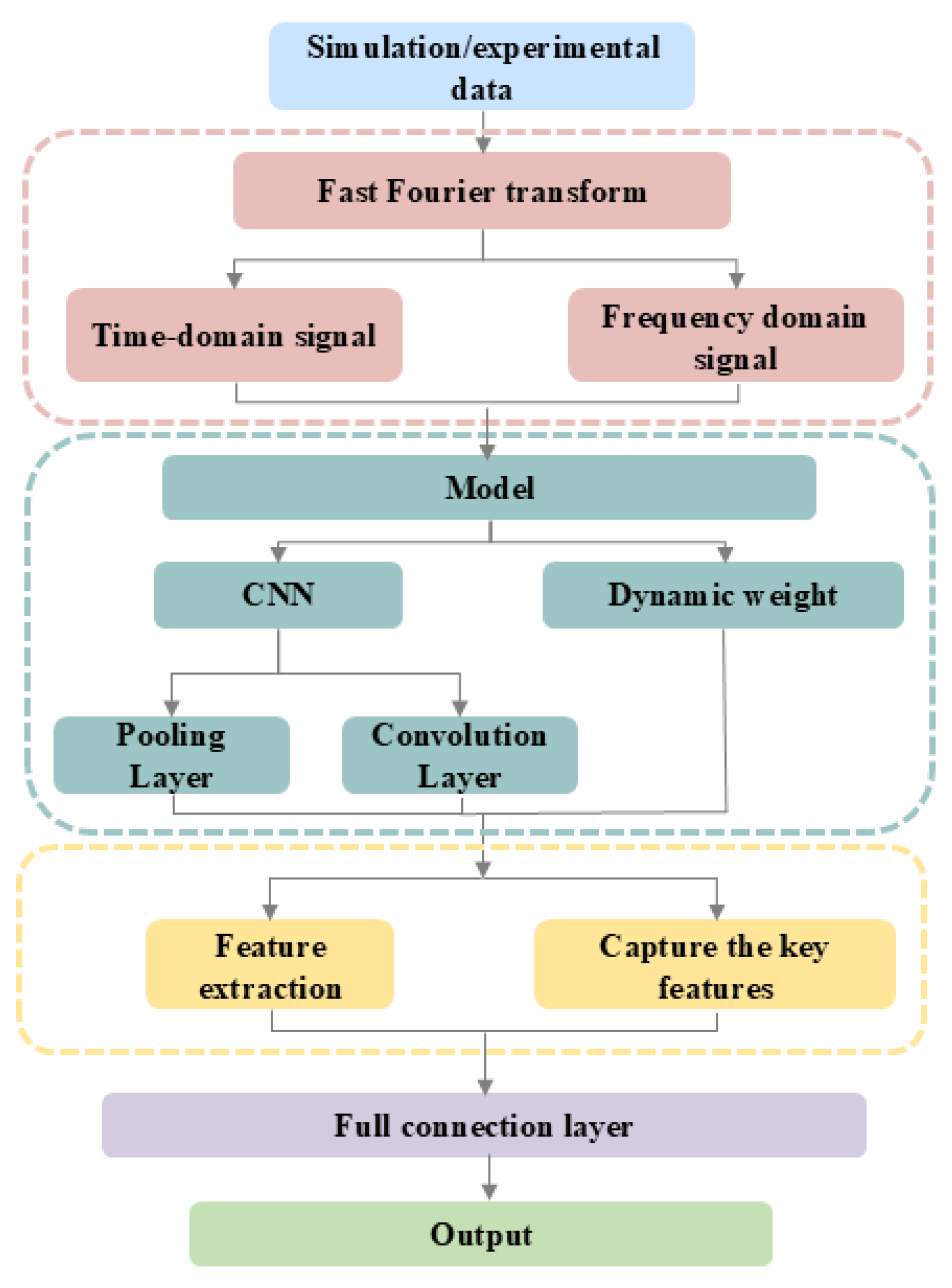
2.2. CNN + Transformer Network Architecture

For signals with non-stationary characteristics, time–frequency methods can simultaneously provide both time and frequency information [36]. For stable signals such as vibration signals of faulty bearings, the FFT can accurately extract the amplitudes and phases of each frequency component. However, the time–frequency method may instead introduce redundant information. There is a lot of environment noise in the time-domain signal, which will make the effective features in the signal blurred. By using the FFT to convert the observed signal into a frequency-domain signal, it is possible to observe more directly which frequency components dominate the signal, which is also conducive to improving the model’s efficiency. The computational complexity of the Discrete Fourier Transform is reduced from O(N²) to O(N logN). The specific process is as shown in Equation (9) as follows:

$$X\left[k\right]=\sum _{n=0}^{N-1}x[n]e^{-j2\pi kn/N}$$

(9)

where e^−j2πkn/N is a complex exponential function, and k is the index in the frequency domain.

A CNN + Transformer transfer learning network is proposed in this paper. The frequency-domain signals of one-dimensional fault signals after FFT transformation and the time-domain features of the signals themselves are extracted for global features through the CNN convolutional pooling layer. Subsequently, the Transformer encoder captures the dependencies in the sequence data. Finally, decisions on classification are made using the fully connected layer. The classification is output through the softmax activation function. The network’s main architecture is shown in Figure 1.

The feature extractor aims to extract the shallow features of the vibration signal, and to extract the shallow features, a convolutional neural network is built. The convolution part is one of the most common CNN models. The convolution layer is the CNN’s core part, and its primary purpose is to extract characteristics from signals. When all the time–frequency signals from the source domain enter the convolution layer, through several convolution kernels of the same size, the convolution operation results of the signal after several convolution kernels can be output. The process of the time–frequency signal passing through the convolutional layer is shown in Equation (10).

$$y\left[n\right]=\sum _{m=0}^{M-1}x\left[n+m-{\displaystyle \frac{M-1}{2}}\right]h[m]$$

(10)

where y[n] represents the output signal value at position n, x[n] represents the input signal value at position n, h[n] is the convolution kernel value at position n, and M is the length of the convolution kernel.

The network can learn complex functional relationships and output accurate prediction results, mostly relying on the nonlinear characteristics of the activation function. When the traditional activation functions Sigmoid (S-shaped function) and tanh (hyperbolic tangent function) input the extreme-value region, the gradient is close to 0, which is prone to causing the vanishing gradient problem and further affecting the training effect of the network. The ReLU (Modified Linear Unit) function can alleviate these situations. The ReLU function is shown in Equation (11).

$$ReLU\left(x\right)=\mathrm{m}\mathrm{a}\mathrm{x}(0,x)$$

(11)

where x is the feature output by the previous convolution layer. The number of samples that need to be trained is relatively large. After the samples undergo convolution and the ReLU function, the maximum feature value of a certain region is selected as the representative through the max pooling layer, effectively compressing the features and reducing the number of training parameters. The max pooling operation is shown in Equation (12).

$$O\left[i\right]=ma{x}_m\left\{I\left[i+m\right]\right\}$$

(12)

where O[i] represents the value of the output feature, I[i + m] represents the input feature value i + m, m represents the offset within the window, and max_m represents the maximum value of the given window.

Furthermore, entering the batch normalization layer can accelerate the training of neural networks. By normalizing the activation values of each batch of data, the problem of internal covariate shift can be reduced. The batch normalization is shown in Equation (13):

$$\left\{\begin{array}{c}{\mu }_B={\displaystyle \frac{1}{m}}\sum _{i=1}^m{x}_i\sigma \\ {\sigma }_B^2={\displaystyle \frac{1}{m}}\sum _{i=1}^m(x_i-{\mu }_B{)}^2\\ {\widehat{x}}_i={\displaystyle \frac{x_i-{\mu }_B}{\sqrt{{\sigma }_B^2+ϵ}}}\\ y_i=\gamma {\widehat{x}}_i+\beta \end{array}\right.$$

(13)

where x_i is the previous layer’s input feature, μ_B is the batch mean, ${\widehat{x}}_i$ is the normalized feature value, γ and β are learnable parameters, and ϵ is a numerically stable tiny positive number. For numerical stability, the parameter is a small positive value.

2.3. Transformer Feature Fusion

2.3.1. Attention Mechanism

The self-attention mechanism is one of the most common attention mechanisms. It correlates the features at different positions in the sequence signal to capture the internal correlations of the data features. The self-attention feature calculates the attention through three parameters (Q, K, V), where Q represents the element being queried, K is the position encoding representing the feature, and V is each element’s value. The specific calculation process of this mechanism is shown in Equation (14):

$$Self-Attention\left(Q,K,V\right)=Softmax({\displaystyle \frac{x{W}_Q(x{W}_K{)}^T}{\sqrt{d_k}}})x{W}_V$$

(14)

where x represents the input feature and d_k is the input layer dimension.

The self-attention mechanism’s capacity to collect effective characteristics is inferior to the CNN’s because it operates on the concept of filtering out significant information and excluding uninteresting information. Only on the basis of extensive datasets can the self-attention mechanism successfully create precise global links. When the dataset is small, its effectiveness is not as good as that of the CNN.

The multi-head attention mechanism achieves different linear transformations of the same input feature by stacking encoding layers. In particular, Q, K and V undergo h linear mappings, each of which takes place simultaneously and produces a distinct output head. Ultimately, to create multi-head attention, all of the output heads are linked and projected. The specific process is shown in Equation (15):

$$\left\{\begin{array}{c}Multihead\left(Q,K,V\right)=Concat(hea{d}_1,\dots ,hea{d}_h)W^O\\ hea{d}_i=Attention(Q{W}_i^Q,K{W}_i^K,V{W}_i^V)\end{array}\right.$$

(15)

The cross-attention mechanism combines these two features with the same input dimension and divides them into two parts. One part serves as the query matrices Q, whose function is to weight the key values of the other input feature to determine how to aggregate the values of this input feature. The attention weights are computed using the key values, and the values are weighted and summed based on these weights to obtain the final output. Equation (16) illustrates the cross-attention mechanism’s computation process:

$$Cross-Attention\left(X_1,X_2\right)=({\displaystyle \frac{X_1{W}_1^Q(X_2{W}_2^K{)}^T}{\sqrt{d_k}}}{X}_2{W}_2^V)$$

(16)

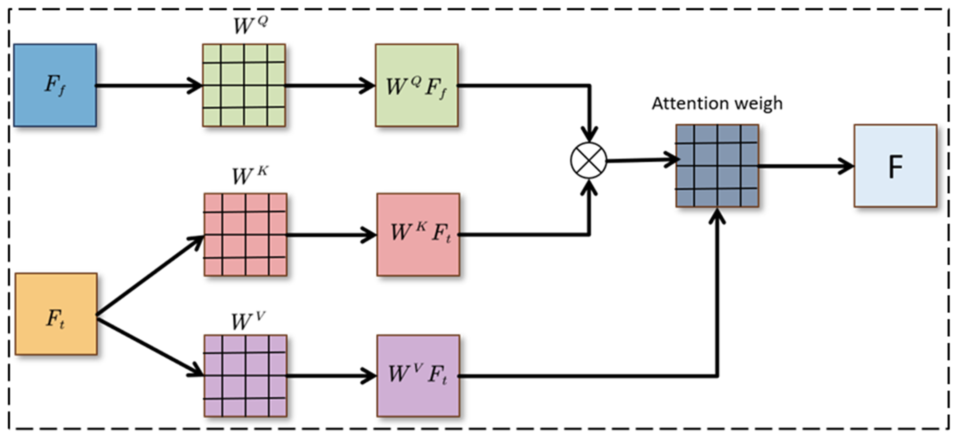
2.3.2. Cross-Attention Mechanism

To emphasize the time-domain characteristics of bearing rotation, it is essential to reduce the influence of external environmental noise. To this end, an attention mechanism is incorporated into the Transformer framework. This mechanism enables the model to focus on the operational signals of the bearing while effectively suppressing external interference. The specific calculation formula is shown in Equation (17):

$$\left\{\begin{array}{c}{F}_t=softmax({\displaystyle \frac{F_{t_K}{F}_{t_Q}^T}{\sqrt{d_t}}})F_{t_V}\\ F_f=softmax({\displaystyle \frac{F_{f_K}{F}_{f_Q}^T}{\sqrt{d_t}}})F_{f_V}\end{array}\right.$$

(17)

where F_f and F_t represent the attention features of the time-domain signal and the frequency-domain signal, respectively, while F_tK, F_tQ and F_tV are all features from the time-domain signal. F_fK, F_fQ and F_fV are all characteristics from frequency-domain signals; d_f and d_t represent the characteristic dimensions of the signals in the frequency domain and the time domain, respectively; softmax represents the activation function.

During the simulation process, when the bearing operates under an ideal state, the time-domain signal will not be disturbed by external factors. However, when the bearing is actually operating, the time-domain signal will be disturbed by external factors, resulting in the time-domain signal containing a lot of other characteristic information. Therefore, to better extract modal information from the time series, a cross-attention mechanism is employed. During this process, the features of each mode are effectively fused to enhance representation quality. Through the cross-attention mechanism’s processing, the model focuses on the relationships between different features to enhance the model’s robustness.

Through the cross-attention mechanism for time-domain and frequency-domain signals, the core of enhancing the anti-interference ability of the fault diagnosis model lies in deeply integrating the complementary advantages of dual-domain features and achieving dynamic adaptive filtering. This mechanism first acquires the time-domain waveform and frequency-domain spectral features through parallel feature extraction channels, and then uses the bidirectional cross-attention weight allocation strategy to construct a dual-domain feature correlation matrix. In this process, external interference signals lack consistent time-domain and frequency-domain correlation. The attention mechanism automatically suppresses their corresponding feature weights. The true fault features, due to their strong time–frequency coupling, will obtain a significant weight increase and form a dynamic perception filter based on feature correlation. Ultimately, this mechanism enhances the cross-domain consistency features and significantly improves the anti-interference ability against external factors.

Figure 2 illustrates the feature fusion module’s operation. The query matrix W^QF_f of F_f is used to calculate the correlation with F_t, thereby calculating the cross-concern of F_f against F_t. This mechanism can enhance the information exchange between the two feature matrices, so as to facilitate better fusion of the information between the two feature matrices. The cross-attention mechanism and the self-attention mechanism may be used to extract the correlations between the points in the sequence. The correlations among the different points in different sequences are different, which can serve as the basis for our classification, as shown in Equation (18):

$$\left\{\begin{array}{c}Cross-Attention\left(F_f,F_t\right)=softmax({\displaystyle \frac{Q_f(K_t{)}^T}{\sqrt{d_k}}})V_t\\ =softmax({\displaystyle \frac{(W^Q{F}_f(W^K{F}_t{)}^T}{\sqrt{d_k}}})W^V{F}_f\end{array}\right.$$

(18)

where W^Q, W^K and W^V are learning parameters; d_k is the query matrix Q dimension. The multi-head attention mechanism is computed multiple times to capture diverse feature representations. The resulting attention outputs from different heads are then superimposed to form a unified representation. A linear transformation is applied to both the superimposed feature representation A_T and the original feature representation A_T. This process yields the final cross-attention feature representation A_ft, which maps frequency-domain features to the time-domain sequence.

$$A_T=Concat(Cross-Attention\left(F_f,F_t\right))$$

(19)

$$A_{ft}=Linear\left(A_T\right)$$

(20)

The resulting feature representation is F when the frequency-domain features are added and combined with the cross-attention mechanism’s time-domain sequence feature representation and the time-domain signal attention feature F_t. On this basis, the attention mechanism is applied to calculate the attention. Through the extraction and fusion of the self-attention mechanism and the cross-attention mechanism, H is the last representation provided to the adaptive layer.

$$\left\{\begin{array}{c}F=A_{ft}+F_t\\ M=tanh(W_m\cdot F+b_m)\end{array}\right.$$

(21)

$$\alpha =softmax(W^T\cdot M)$$

(22)

$$H=F\cdot {\alpha }^T$$

(23)

where W_m denotes the weight matrix corresponding to the attention mechanism layer depth, W_T is the initialization parameter random matrix, b_m is the bias vector, and α is the input assignment weight.

2.3.3. Domain Adaptive Classifier

This paper introduces an adaptive fusion module designed to integrate self-attention and cross-attention features, aiming to remove redundant information across different feature sets. The adaptive fusion process consists of three main stages: global average pooling (GAP), feature compression, and feature expansion. Initially, the input feature undergoes GAP to produce the feature vector Z. Subsequently, Z is linearly transformed and compressed to one quarter of its original dimension, yielding the compressed vector Z_cmps:

$$Z_{cmps}=ReLU\left(FC\left(Z,W_{cmps}\right)\right),Z_{cmps}\in R^{{\displaystyle \frac{n}{4}}}$$

(24)

where ReLU stands for the nonlinear activation function and FC for the fully connected layer. Since W_cmps is a learnable parameter, dynamically modifying the parameter during the backpropagation process can reduce the redundant information among the feature sets. Finally, the features are mapped to the 0–1 interval through the Sigmoid activation function, and the fusion weights of the learned feature matrix and the original feature matrix are multiplied:

$$Z_{exc}=\phi \left(FC\left(Z_{cmps},W_{exc}\right)\right),Z_{exc}\in R^n$$

(25)

where W_exc is the expansion coefficient and $\phi \left(x\right)={\displaystyle \frac{1}{1+e^{-x}}}$ represents the Sigmoid activation function.

Figure 3 depicts the flowchart of the proposed method. Firstly, a bearing fault dynamics model is established, and it is solved using the Runge–Kutta theory. The obtained simulation/experiment data is subjected to Fast Fourier Transform to obtain frequency-domain signals with fault characteristics. The time–frequency signals are processed through the CNN module to obtain global features. The cross-attention mechanism captures the global features extracted by the CNN module. Based on the dynamic weight allocation, larger weights are assigned to the signals with more obvious fault features. Finally, the precise classification results are output.

3. Dynamics Simulation and Experimental Verification

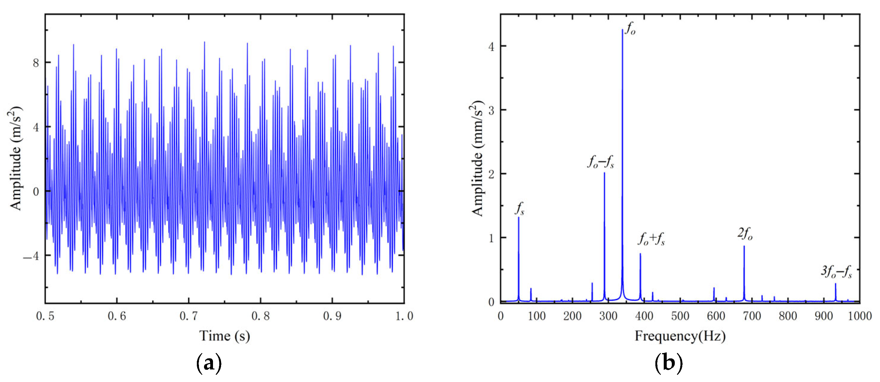
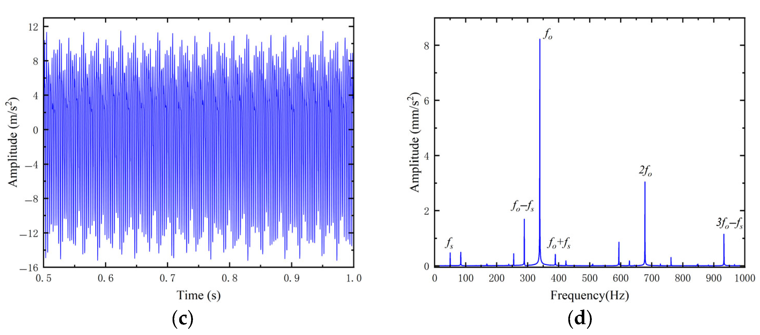
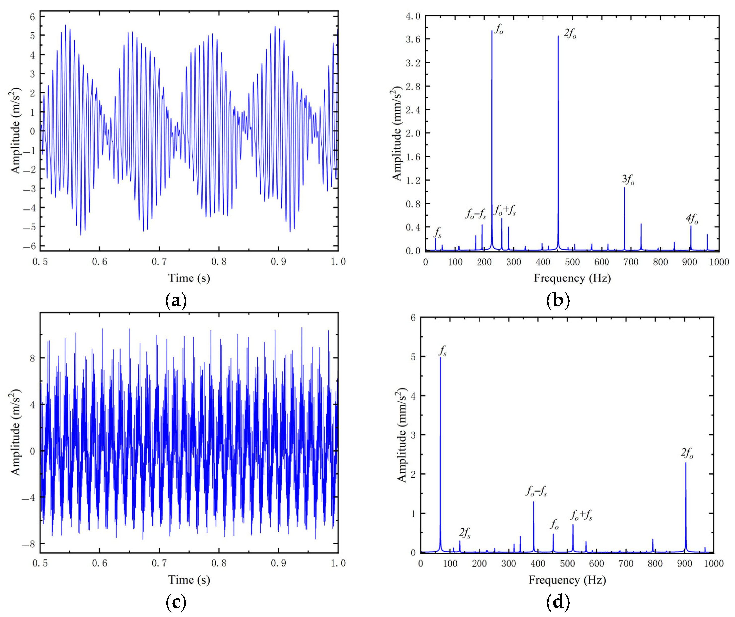
3.1. Dynamics Simulation Analysis

In this simulation, the 7008CE bearing (Svenska Kullager-Fabriken, Dalian, China) is used. The assumed width is 1 mm. The fault is located on the bearing outer raceway. The vibration characteristics at 3000 rpm are shown in Figure 4. As seen in Figure 4a, when the outer ring has a single point of failure, there is a distinct shock response in the time-domain waveform. As seen in Figure 4b, in addition to the rotation frequency, the outer ring fault characteristic frequencies and their combined frequencies appear in the spectrum diagram. The outer ring fault theoretical characteristic frequency of this bearing is 340.85 Hz, and the simulation characteristic frequency is 339.05 Hz, which differs from the theoretical frequency domain by 1.8 Hz. The axis trajectory is rather chaotic, and the motion state of the bearing is rather complex. The phase trajectory is composed of multiple irregular closed curves, and chaotic attractors of multiple periods appear in the Poincare section.

Figure 5 shows the time–frequency-domain graphs of different fault widths at 3000 rpm. It can be seen that as the width of the fault increases, the amplitude of the vibration becomes larger, the amplitude of the fault characteristic frequency becomes more obvious, and the impact characteristics become more obvious. This is because the increase in the size of the fault causes the internal excitation force of the bearing to increase, thereby changing its vibration characteristics. However, it will not affect the fault characteristic frequency of the bearing and the magnitude of its multiples.

The time–frequency-domain graphs of the bearing’s steady-state vibration response at various speeds and time intervals are displayed in Figure 6. With an increase in speed, the vibration period shortens, the time domain becomes a more complex multi-period trigonometric function, and the fluctuation becomes intense. The amplitude of the rotation frequency becomes larger and gradually takes the dominant position. This is because the centrifugal force of the bearing increases with an increase in the speed. Additionally, when speed rises, so does the vibration amplitude.

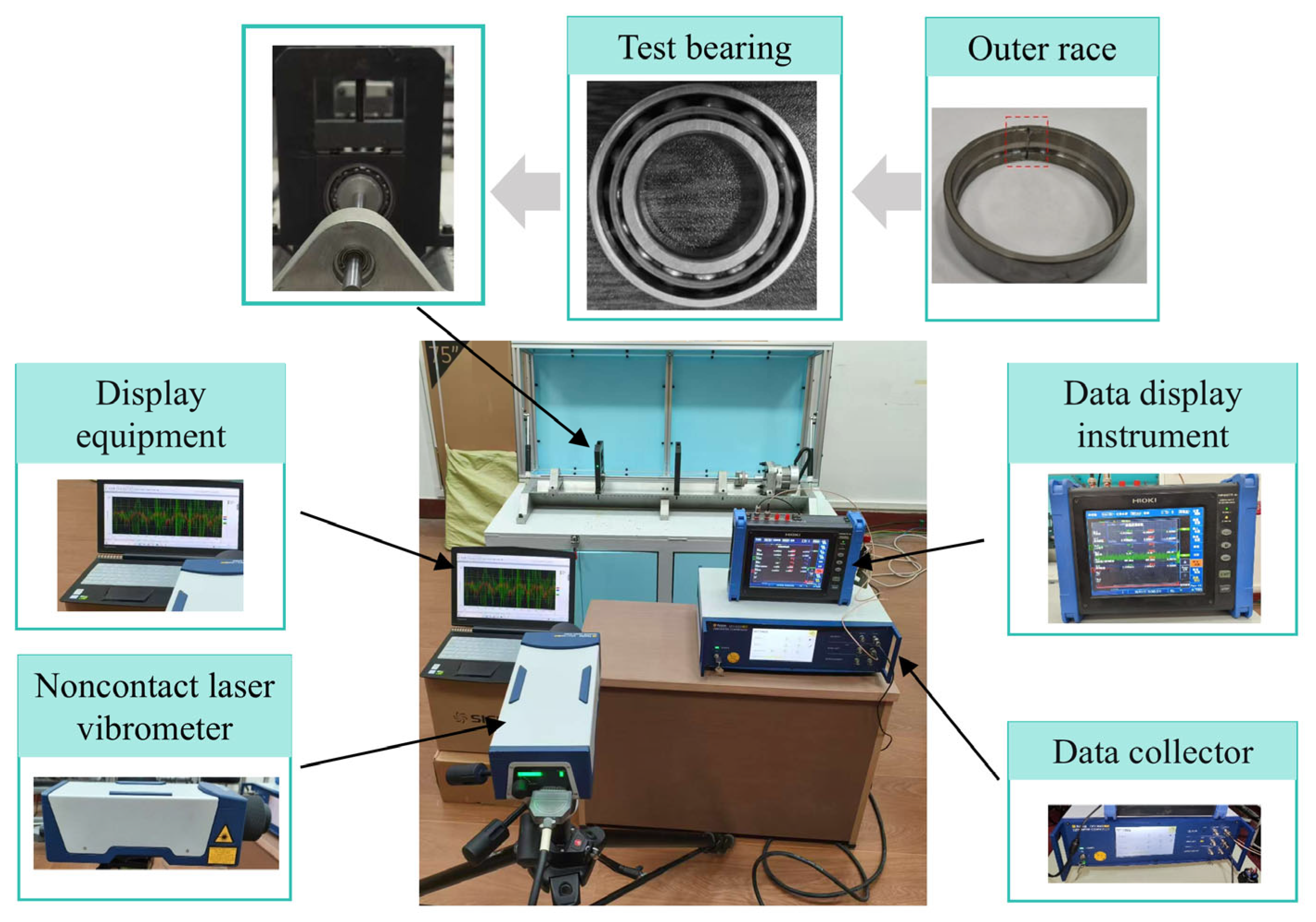
3.2. Experiment Setup

Four distinct health states’ bearing data are included in the simulation dataset: health state (N), fault width 0.5 mm (IF), fault width 1 mm (OF), and fault width 2 mm (R). We classified the bearing states into four categories based on the fault width. Each state of the bearing contains 236 samples, and each sample contains 1024 data points. To capture the highest correlation among samples in the time series, a sliding window with a 0.5 overlap ratio is applied. The dataset is then partitioned into training, validation, and test sets in a 7:2:1 ratio. The experimental setting environment is as follows: The GPU is NVIDIA RTX 4090 (NVIDIA Corporation, Santa Clara, CA, USA), the CPU is Intel i9-14900KF (Intel Corporation, Santa Clara, CA, USA), and the running environment is the python3.8 pytorch framework. The model is trained with an initial learning rate of 0.001, over 50 epochs, using a batch size of 32.

The bearing data were gathered using the high-speed bearing–rotor test platform depicted in Figure 7 in order to confirm the correctness of the suggested model. According to the requirements of the experimental verification,

Table 1. Introduction to data details.

Healthy State	Label	Sample Number
N	0	238
IR	1	236
OR	2	235
R	3	237

provides a thorough overview of the data used. The test platform is composed of a laser acquisition instrument, a data acquisition instrument, a drive motor and a bearing test platform. The vibration of the system was measured using a German Polytec OFV-505 (Polytec GmbH, Waldbronn, Germany) non-contact laser vibrometer. Data acquisition was performed with a HIOKI MR8875-30 data logger (Hioki E.E. Corporation, Nagano, Japan). The sampling frequency was 20 kHz. The rated power of the motor is 11 kW, the maximum current of the motor is 22.3 A, and the rated torque of the motor is 7 N·m. The speed was set to 2000 r/min. The model’s generality was confirmed by extracting the simulation and experimental signals, and the data can also further validate the model. Due to limitations in experimental conditions, signals collected experimentally contain more noise than simulated signals.

Figure 8 displays the model’s accuracy curve. When the training begins, when the quantity of iterations rises, the model continuously optimizes until it converges. When the model passes through the 20th epoch, the accuracy rate can be stably above 95%, and the loss function shows a downward trend, proving the robustness of the method we proposed. Furthermore, we have also drawn the confusion matrix of the classification task and the t-SNE visualization classification diagram, as shown in Figure 9. As shown in Figure 9, the method proposed in this paper achieves high classification accuracy. This further demonstrates the robustness and effectiveness of the proposed approach. Extensive training was performed using simulation and experimental data to determine hyperparameter values. Their specific values are shown in

Table 2. The structural parameters of the network model.

Module	Layer	Parameters	Output Shape	Comment
Input Layer	Original Signal		(32, 1, 1024)	Batch Size = 32 Signal = 1024
	FFT		(32, 1, 512)
CNN	Convolution 1	(2, 16)	(32, 16, 512)
	Convolution 2	(2, 32)	(32, 32, 512)
	Convolution 3	(1, 64)	(32, 64, 128)
Transformer (Attention)	Input Dimension	64	(32, 128, 64)
	Encoder Layer	2	(32, 128, 64)
	Attention Head	4	(32, 128, 64)

.

To further verify the generalization of the proposed method under actual operating conditions, radial loads of 200 N, 500 N and 1000 N were applied to the bearing using an experiment platform. Data collected under these three different radial loads were used for validation. As shown in Figure 10, confusion matrices and t-SNE visualization plots show that our method has excellent generalization ability.

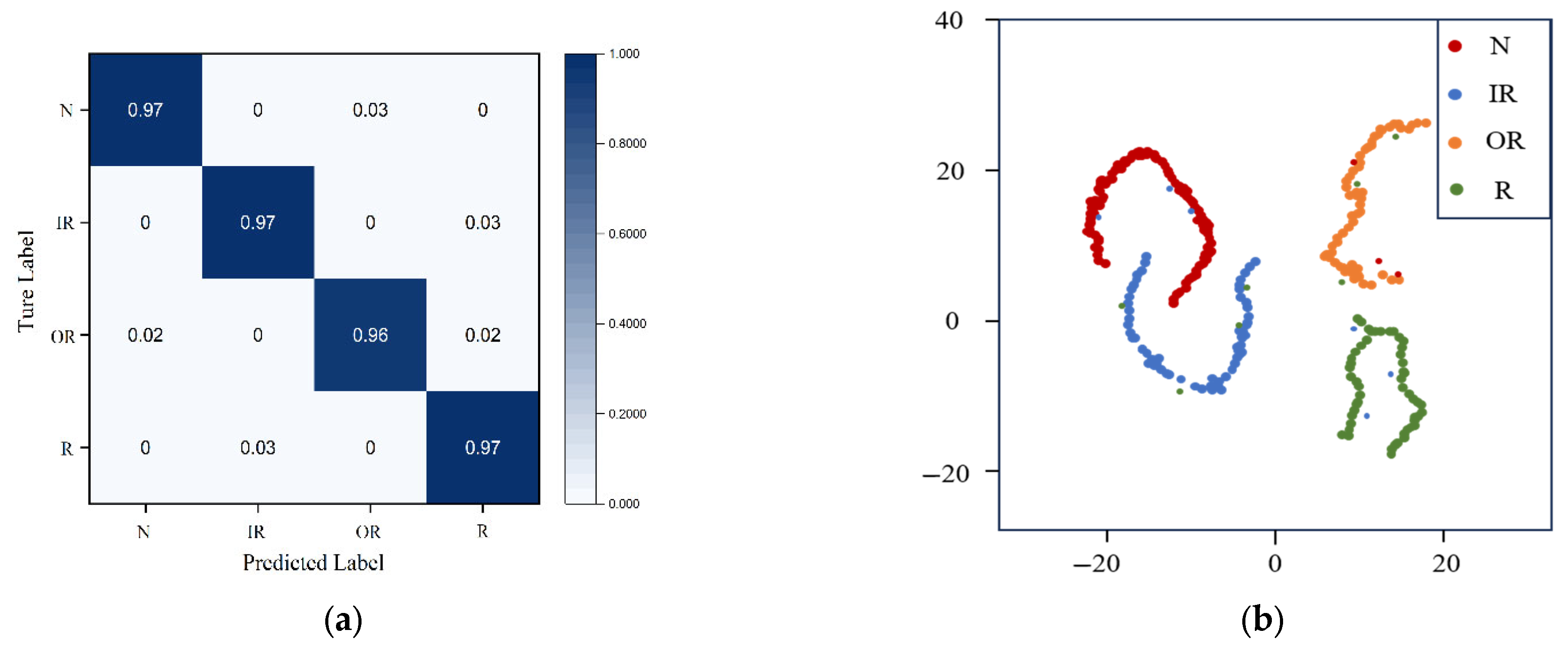
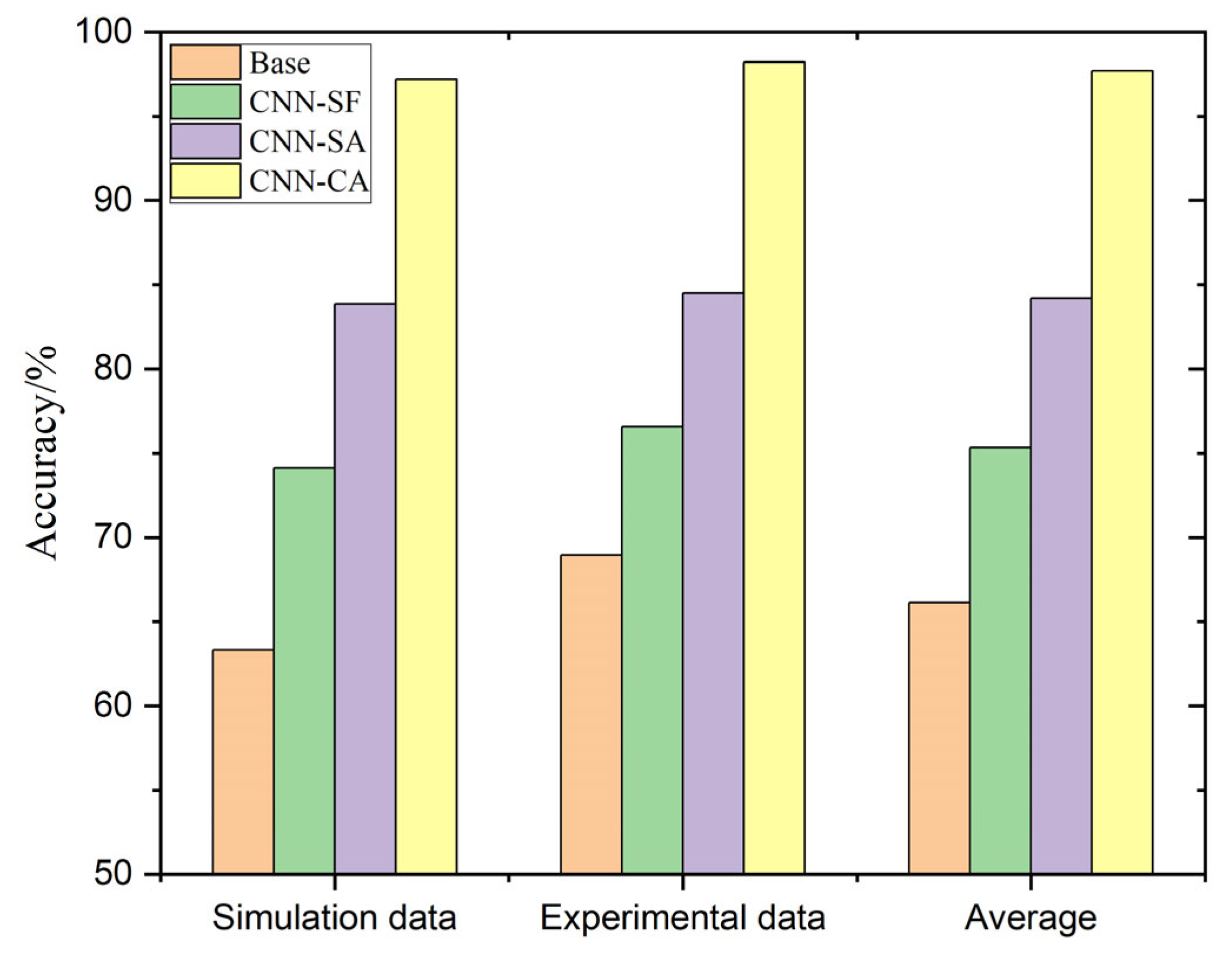
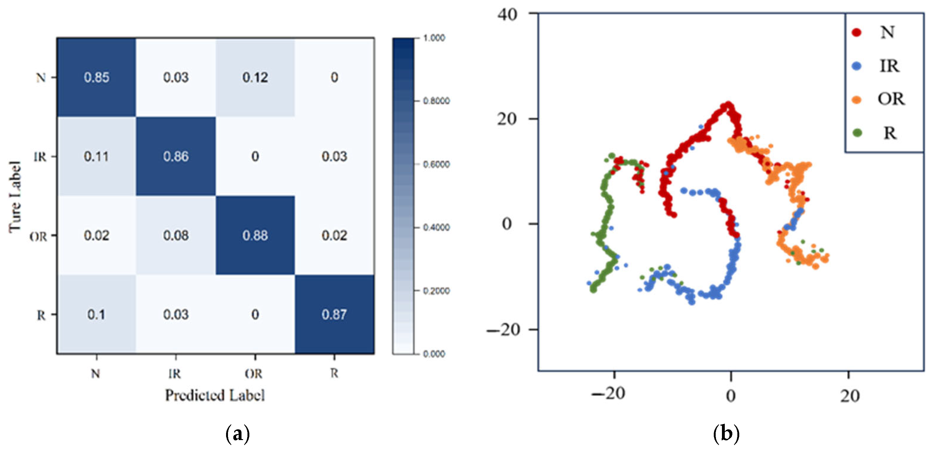
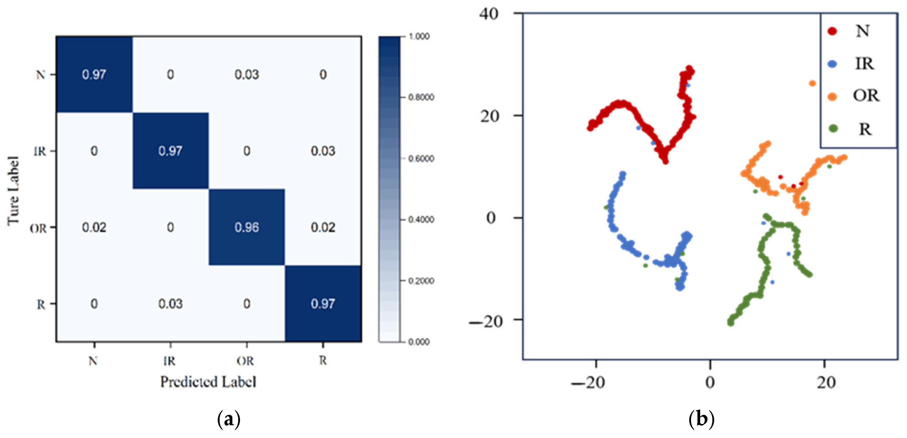
3.3. Method Comparison

To further evaluate the validity of the model, three methods were adopted to compare with the method proposed in this section. The comparison results are shown in Figure 11, where Base represents the method proposed in this paper. Although the verification accuracy rates of all four methods can reach over 80%, it can be seen from the comparison result graph that the method proposed in this paper is superior to the other methods. To verify the effectiveness of dynamic weight allocation, an ablation study was designed. The baselines include Base (a basic CNN), CNN-SF (CNN with static fusion), CNN-SA (CNN with self-attention mechanism) and CNN-CA (our proposed method). Both experimental and simulation data validate the method. Figure 12 shows that cross-attention with dynamic weights achieves higher accuracy. Other methods, without dynamic weights, have relatively lower accuracy. This ablation study further confirms that CNN-CA outperforms other CNN-fused methods in accuracy.

In order to see the comparison results more intuitively, we drew the confusion matrices of ResNet, BiLSTM and CNN and the t-SNE classification visualization diagrams. As shown in Figure 13, although the classification result of the ResNet method reaches 90%, compared to the approach proposed in this study, it is marginally worse. Although the residual structure of ResNet can alleviate the vanishing gradient problem and extract deep features, its fixed skip connection mechanism lacks the ability of dynamic feature interaction. It is difficult to adaptively capture the complex correlations among multi-sensor signals or features of different frequency bands like the cross-attention mechanism. ResNet has a relatively weak ability to model the global context of multi-scale fault features in the feature fusion stage. However, cross-attention can more effectively integrate local details and global dependencies through the interaction between feature channels/spaces, especially having a stronger recognition ability for weak fault signals and time-varying features under non-stationary working conditions.

As shown in Figure 14, although the classification accuracy of BiLSTM has reached more than 80%, it can be seen from t-SNE that the classification results are relatively poor and the classification points are relatively scattered. Although BiLSTM can effectively model the long-term bidirectional dependency relationship of temporal signals, its recursive structure lacks the inherent local spatial feature extraction ability of CNN when dealing with high-dimensional and multi-channel sensor signals, making it difficult to efficiently capture the key local patterns in fault signals. The serial computing characteristics of BiLSTM lead to its low efficiency in parallelization processing of long sequence data.

As shown in Figure 15, the classification of the CNN not only has a lot of confusion but also has a classification accuracy rate lower than 80%, and the classification points are particularly scattered. Although the CNN can effectively extract local spatial features through convolutional layers, its fixed receptive field and static weight allocation mechanism cause difficulty in adaptively focusing on the key fault areas. The cross-attention mechanism can enhance the representation ability of weak fault features through dynamic weight adjustment. The hierarchical stacking structure of the CNN is prone to losing fine-grained fault information in deep networks, while cross-attention, through bidirectional information fusion between feature maps, can integrate local details and global dependencies more robustly.

Furthermore, in order to further verify this generalization method, as shown in Figure 16, we verified it using simulation data, and the accuracy rate reached more than 95%.

4. Conclusions

In this paper, aiming to solve the problems of insufficient utilization of time–frequency features in bearing FD and the weak interaction ability of dynamic features in traditional models, a deep dynamic learning network based on dual-channel cross-attention of time–frequency signals is proposed. By establishing the faulty bearing’s dynamic model, the simulated vibration signal is obtained and decomposed into dual-channel features in the time domain and frequency domain through the FFT. Combined with the CNN, local and global features are extracted, and a cross-attention mechanism is designed to achieve the dynamic interaction and weight distribution of features in the time domain and frequency domain. It significantly enhances the model’s sensitivity to weak fault characteristics and robustness under noise interference. The experimental results show that in the simulation dataset and the data of the self-built bearing test platform, the proposed method is superior to ResNet, BiLSTM and the traditional CNN model in terms of accuracy (above 95%) and classification stability. Especially under non-stationary working conditions, it effectively reduces the misjudgment rate through the complementarity of time–frequency features. Furthermore, the introduction of domain adaptive classifiers further optimizes the feature fusion process and reduces the interference of redundant information. This study validates the effectiveness of the cross-attention mechanism for cross-modal feature fusion. The findings offer a novel approach to IFD in complex industrial environments.

References

1. Shang, L.; Zhang, Z.; Tang, F.; Cao, Q.; Pan, H.; Lin, Z. CNN-LSTM hybrid model to promote signal processing of ultrasonic guided lamb waves for damage detection in metallic pipelines. Sensors 2023, 23, 7059. [Google Scholar] [CrossRef]
2. Zhao, Y.; Zhang, N.; Zhang, Z.; Xu, X. Bearing fault diagnosis based on mel frequency cepstrum coefficient and deformable space-frequency attention network. IEEE Access 2023, 11, 34407–34420. [Google Scholar] [CrossRef]
3. Zegai, M.L.; Bendjebbar, M.; Belhadri, K.; Doumbia, M.L.; Hamane, B.; Koumba, P.M. Direct torque control of Induction Motor based on artificial neural networks speed control using MRAS and neural PID controller. In Proceedings of the 2015 IEEE Electrical Power and Energy Conference (EPEC), London, ON, Canada, 26–28 October 2015; pp. 320–325. [Google Scholar] [CrossRef]
4. Douiri, M.R.; Cherkaoui, M.; Douiri, S.M. Rotor resistance and speed identification using extended kalman filter and fuzzy logic controller for induction machine drive. In Proceedings of the 2012 International Conference on Multimedia Computing and Systems, Tangiers, Morocco, 10–12 May 2012; pp. 1182–1187. [Google Scholar] [CrossRef]
5. Douiri, M.R.; Cherkaoui, M.; Nasser, T.; Essadki, A. A neuro fuzzy PI controller used for speed control of a direct torque to twelve sectors controlled induction machine drive. In Proceedings of the 2011 International Conference on Multimedia Computing and Systems, Ouarzazate, Morocco, 7–9 April 2011; pp. 1–6. [Google Scholar] [CrossRef]
6. Chen, Z.; Yang, Y.; He, C.; Liu, Y.; Liu, X.; Cao, Z. Feature extraction based on hierarchical improved envelope spectrum entropy for rolling bearing fault diagnosis. IEEE Trans. Instrum. Meas. 2023, 72, 1–12. [Google Scholar] [CrossRef]
7. Wang, Z.; Li, G.; Zhou, X.; Zhang, H.; Lin, Z.; Jia, S. Dynamic analysis of deep groove ball bearing with localized defects and misalignment. J. Sound Vib. 2024, 568, 118071. [Google Scholar] [CrossRef]
8. Liu, K.; Wang, D.; Chen, B.; Shi, X.; Feng, Y.; Li, W. Vibration characteristics investigation of a single/dual rotor-bearing-casing system with local bearing defects. Mech. Syst. Signal Process. 2025, 225, 112227. [Google Scholar] [CrossRef]
9. Jafari, S.M.; Rohani, R.; Rahi, A. Experimental and numerical study of an angular contact ball bearing vibration response with spall defect on the outer race. Arch. Appl. Mech. 2020, 90, 2487–2511. [Google Scholar] [CrossRef]
10. Alkomy, H.; Shan, J. Modeling and validation of reaction wheel micro-vibrations considering imbalances and bearing disturbances. J. Sound Vib. 2021, 492, 115766. [Google Scholar] [CrossRef]
11. Dipen, S.S.; Patel, V.N. Theoretical and experimental vibration studies of lubricated deep groove ball bearings having surface waviness on its races. Measurement 2018, 129, 405–423. [Google Scholar] [CrossRef]
12. Larizza, F.; Howard, C.Q.; Grainger, S.; Wang, W. A nonlinear dynamic vibration model of a defective bearing: The importance of modelling the angle of the leading and trailing edges of a defect. Struct. Health Monit. 2020, 20, 2604–2625. [Google Scholar] [CrossRef]
13. Mufazzal, S.; Muzakkir, S.M.; Khanam, S. Theoretical and experimental analyses of vibration impulses and their influence on accurate diagnosis of ball bearing with localized outer race defect. J. Sound Vib. 2021, 513, 116407. [Google Scholar] [CrossRef]
14. Tingarikar, G.; Choudhury, A. Vibration analysis-based fault diagnosis of a dynamically loaded bearing with distributed defect. Arab. J. Sci. Eng. 2021, 47, 8045–8058. [Google Scholar] [CrossRef]
15. Govardhan, T.; Choudhury, A. Amplitudes of components in vibration spectra of rolling bearings with localized defects under harmonic loads. J. Vib. Control 2020, 27, 1537–1547. [Google Scholar] [CrossRef]
16. Luo, M.; André, H.; Guo, Y.; Peng, Y. Analysis of contact behaviours and vibrations in a defective deep groove ball bearing. J. Sound Vib. 2024, 570, 118104. [Google Scholar] [CrossRef]
17. Zhang, X.; Bai, C.; Jin, Y.; Wang, J. Nonlinear vibration characteristics of a rotor bearing system with irregular raceway defect. Nonlinear Dyn. 2025, 113, 11259–11281. [Google Scholar] [CrossRef]
18. Song, X.; Li, Z.; Liu, Y. MVB fault diagnosis based on time-frequency analysis and convolutional neural networks. Sci. Rep. 2025, 15, 5271. [Google Scholar] [CrossRef] [PubMed]
19. Zhang, P.; Chen, R.; Yang, L.; Zou, Y.; Gao, L. Recent progress in digital twin-driven fault diagnosis of rotating machinery: A comprehensive review. Neurocomputing 2025, 634, 129914. [Google Scholar] [CrossRef]
20. Han, T.; Zhang, L.; Yin, Z.; Tan, A.C. Rolling bearing fault diagnosis with combined convolutional neural networks and support vector machine. Measurement 2021, 177, 109022. [Google Scholar] [CrossRef]
21. Chen, S.; Yang, R.; Zhong, M. Graph-based semi-supervised random forest for rotating machinery gearbox fault diagnosis. Control Eng. Pract. 2021, 117, 104952. [Google Scholar] [CrossRef]
22. Wang, X.; Gu, H.; Wang, T.; Zhang, W.; Li, A.; Chu, F. Deep convolutional tree-inspired network: A decision-tree-structured neural network for hierarchical fault diagnosis of bearings. Front. Mech. Eng. 2021, 16, 814–828. [Google Scholar] [CrossRef]
23. Lee, D.; Choo, H.; Jeong, J. Gcn-based lstm autoencoder with self-attention for bearing fault diagnosis. Sensors 2024, 24, 4855. [Google Scholar] [CrossRef]
24. Borré, A.; Seman, L.O.; Camponogara, E.; Stefenon, S.F.; Mariani, V.C.; Coelho, L.d.S. Machine fault detection using a hybrid CNN-LSTM attention-based mode. Sensors 2023, 23, 4512. [Google Scholar] [CrossRef] [PubMed]
25. Djaballah, S.; Saidi, L.; Meftah, K.; Hechifa, A.; Bajaj, M.; Zaitsev, I. A hybrid LSTM random forest model with grey wolf optimization for enhanced detection of multiple bearing faults. Sci. Rep. 2024, 14, 23997. [Google Scholar] [CrossRef] [PubMed]
26. Thuan, N.D. A novel bearing fault diagnosis method for compound defects via zero-shot learning. J. Mech. Sci. Technol. 2024, 38, 4603–4610. [Google Scholar] [CrossRef]
27. Hassannejad, R.; Ettefagh, M.M.; Mossayebi, Y.B. Adaptive wavelet-informed physics-based CNN for bearing fault diagnosis. Int. J. Progn. Health Manag. 2025, 16, 1–20. [Google Scholar] [CrossRef]
28. Gao, H.; Ma, J.; Zhang, Z.; Cai, C. Bearing fault diagnosis method based on attention mechanism and multi-channel feature fusion. IEEE Access 2024, 12, 45011–45025. [Google Scholar] [CrossRef]
29. Li, Y.; Men, Z.; Bai, X.; Xia, Q.; Zhang, D. A bearing fault diagnosis method based on M-SSCNN and M-LR attention mechanism. Struct. Health Monit. 2025, 24, 830–852. [Google Scholar] [CrossRef]
30. Lee, S.K.; Kim, H.; Chae, M.; Oh, H.J.; Yoon, H.; Youn, B.D. Self-supervised feature learning for motor fault diagnosis under various torque conditions. Knowl.-Based Syst. 2024, 288, 111465. [Google Scholar] [CrossRef]
31. Kim, Y.; Kim, Y.K. Physics-informed time-frequency fusion network with attention for noise-robust bearing fault diagnosis. IEEE Access 2024, 12, 12517–12532. [Google Scholar] [CrossRef]
32. Snyder, Q.; Jiang, Q.; Tripp, E. Integrating self-attention mechanisms in deep learning: A novel dual-head ensemble transformer with its application to bearing fault diagnosis. Signal Process. 2025, 227, 109683. [Google Scholar] [CrossRef]
33. Chen, Y.; Shi, J.; Hu, J.; Shen, C.; Huang, W.; Zhu, Z. Simulation data driven time-frequency fusion 1D convolutional neural network with multiscale attention for bearing fault diagnosis. Meas. Sci. Technol. 2025, 36, 035109. [Google Scholar] [CrossRef]
34. Hou, W.; Zhang, C.; Jiang, Y.; Cai, K.; Wang, Y.; Li, N. A new bearing fault diagnosis method via simulation data driving transfer learning without target fault data. Measurement 2023, 215, 112879. [Google Scholar] [CrossRef]
35. Xie, J.; Tian, L.; Lin, M.; Yang, B.; Yang, J.; Wang, T. A small sample diagnosis method driven by simulation and test data: Applied to axle box bearings of high-speed train. Meas. Sci. Technol. 2023, 34, 125044. [Google Scholar] [CrossRef]
36. Elouaham, S.; Latif, R.; Nassiri, B.; Dliou, A.; Laaboubi, M.; Maoulainine, F. Analysis electroencephalogram signals using ANFIS and periodogram techniques. Int. Rev. Comput. Softw. 2013, 8, 2959–2966. [Google Scholar]
Figure 1. The network’s main architecture.
Applsci 15 07908 g001
Figure 2. Cross-attention mechanism.
Applsci 15 07908 g002
Figure 3. The flowchart of the proposed method.
Applsci 15 07908 g003
Figure 4. Dynamic characteristics of the bearing at 3000 rpm: (a) time domain, (b) frequency domain, (c) shaft center trajectory, (d) blue lines are phase trajectory and red crosses are Poincare mapping.
Applsci 15 07908 g004
Figure 5. Vibration under different fault widths: (a) 0.5 mm time domain, (b) 0.5 mm frequency domain, (c) 2 mm time domain, (d) 2 mm frequency domain.
Applsci 15 07908 g005aApplsci 15 07908 g005b
Figure 6. Vibration at different rotational speeds: (a) 2000 rpm time domain, (b) 2000 rpm frequency domain, (c) 4000 rpm time domain, (d) 4000 rpm frequency domain.
Applsci 15 07908 g006
Figure 7. Experiment platform for bearing–rotor system.
Applsci 15 07908 g007
Figure 8. Model accuracy curve.
Applsci 15 07908 g008
Figure 9. (a) The model confusion matrix; (b) the t-SNE visualization diagram.
Applsci 15 07908 g009
Figure 10. The model confusion matrix and the t-SNE visualization diagram: (a,b) 200 N, (c,d) 500 N (e,f) 1000 N.
Applsci 15 07908 g010
Figure 11. Comparison chart of the accuracy rates of four different models, blue represents Base, purple represents CNN, red represents BiLSTM, and yellow represents ResNet.
Applsci 15 07908 g011
Figure 12. Accuracy comparison.
Applsci 15 07908 g012
Figure 13. (a) ResNet confusion matrix; (b) t-SNE visualization diagram.
Applsci 15 07908 g013
Figure 14. (a) BiLSTM confusion matrix; (b) visualization diagram.
Applsci 15 07908 g014
Figure 15. (a) CNN confusion matrix; (b)visualization graph.
Applsci 15 07908 g015
Figure 16. (a) The confusion matrix of the simulation data; (b) the t-SNE visualization classification diagram.
Applsci 15 07908 g016