1. Introduction
Time series data mining has applications in many areas [
1,
2]. Time series are commonly used for data classification, fault detection, pattern recognition, and prediction [
3]. However, supervised methods such as convolutional neural networks (CNNs) are not suitable for datasets with non-uniform lengths [
4]. The Hidden Markov Model (HMM) can adapt to some datasets, but its performance is poor [
5,
6]. Recurrent Neural Networks (RNNs) can also be used to process temporal data, but there are problems of long training time and difficulty in convergence [
7]. The SBD (Shape-Based Distance) algorithm has the advantages of high computational efficiency, ease of comparison, and strong adaptability [
8]. The SBD algorithm is currently mainly applied in the fields of time series clustering, anomaly detection, etc. [
9].
With the rapid development of the coal industry in China, the intensity of mining in mines continues to rise, resulting in frequent non-natural seismic events during the mining process, which seriously threaten the life and property safety of on-site workers. According to the monitoring data released by the Seismic Network of Shandong Province, 337 natural seismic events and 561 non-natural seismic events were monitored in 2020; 304 natural seismic events and 269 non-natural seismic events occurred in 2021. The frequency of non-natural seismic events has clearly surpassed that of natural seismic events. Therefore, it is very important to identify and classify microseismic events in a timely and accurate manner [
10], providing an important guarantee for the production safety of coal mines [
11]. Domestic and foreign research on coal mine microseismic events mainly focuses on the focal mechanism [
12], the optimization of the microseismic sensor network, etc. [
13], while research on the identification of microseismic events is relatively insufficient. Recent studies have focused on unsupervised representation learning for seismic data [
14] and lightweight architectures for real-time detection [
15], yet challenges remain in robust shape-based similarity metrics under noisy conditions [
16].
The motivation for this study stems from the urgent need to improve the classification and clustering of microseismic events—particularly in distinguishing between microseisms, blasting events, and background noise. In mining environments, the ability to accurately and efficiently identify such events is crucial for ensuring operational safety and optimizing early warning systems [
17]. However, the waveform signals of different microseismic events often exhibit highly similar characteristics, making classification a challenging task [
18]. Moreover, the presence of noise and the lack of labeled datasets further complicate traditional analytical approaches [
19].
The research on microseismic waveform identification began in the 1960s and initially relied on manual observation, but this method was inefficient. Over time, scholars at home and abroad have developed various microseismic waveform identification techniques. For example, researchers such as Chen Anguo reviewed the existing microseismic identification technologies [
20]; Feng Tian et al. developed a microseismic signal identification method based on the VGG4-CNN model, which requires data to be labeled manually [
21]. In addition, Li Jiaming et al. improved the LeNet5 convolutional neural network and proposed a new microseismic monitoring waveform identification technology [
22]. Pan Yishan et al. further classified microseismic waveforms into categories such as coal compression type, roof fracture type, and fault dislocation type for detailed research [
23]. To solve the practical problems of large fluctuations in the accuracy of conventional mathematical methods when disturbed by noise and over-reliance on labels by supervised learning methods, this paper proposes a new unsupervised learning method. Based on the classic Shape-Based Distance (SBD) algorithm, a multi-scale fusion spatial convolutional autoencoder is proposed for feature extraction of the original waveform. The introduction of a time-limited window enables the SBD algorithm to better help two microseismic waveforms find corresponding points, thereby improving the calculation speed of the SBD algorithm, and a SBD algorithm that fuses volatility is proposed to further improve the accuracy and robustness of the proposed algorithm.
2. Related Technologies
2.1. Deep Learning
Deep learning, as a machine learning technology based on artificial neural networks, relies on multi-level network architectures to conduct hierarchical extraction and transformation of data, thereby constructing more advanced and abstract data representations [
24]. This technology has the ability to automatically identify features from a large number of unlabeled data in an unsupervised or semi-supervised environment. At the same time, in a supervised environment, it optimizes network parameters by using labeled data. Deep learning has shown unique advantages in dealing with high-dimensional, nonlinear, and complex data and is able to excavate the potential rules and structures within the data. In multiple fields such as computer vision [
25], speech recognition [
26], natural language processing [
27], and bioinformatics [
28], deep learning has demonstrated outstanding achievements and has become one of the key technologies promoting the development of artificial intelligence.
2.2. Convolutional Neural Network
The deep neural network that uses convolution kernels to extract local features from input data is called the convolutional neural network. It is characterized by the interleaving of convolutional layers and pooling layers and is equipped with one or more fully connected layers at the end. Through the convolution layer, this network can grasp the spatial layout of the data and the stability of its migration; with the help of the pooling layer, the scale and complexity of the data can be simplified; and the fully connected layer is responsible for completing various tasks such as classification and regression [
29]. In multiple fields such as image recognition and speech processing, convolutional neural networks have demonstrated their wide applicability and excellent performance.
2.3. Convolutional Autoencoder
The neural network architecture that simplifies and reproduces data through convolution operations is called the convolutional autoencoder [
30], including the convolutional encoding part responsible for compressing the data to a low-dimensional space and the convolutional decoding part responsible for restoring these data to the original state. This model is particularly good at capturing the spatial layout and characteristics of the data, making it very suitable for processing high-dimensional content such as images and videos. In terms of specific applications, convolutional autoencoders perform well in tasks such as image denoising, image creation, and feature extraction.
2.4. SBD Algorithm
The Shape-Based Distance (SBD) algorithm is an algorithm used to compare and measure the similarity of time series. It effectively handles time series with variations in speed and length on the time axis. The basic idea is to align two time series by finding an optimal alignment to maximize their similarity on the timeline.
First, we define the distance metric function between two time series and as , representing the distance between the i-th data point of the time series X and the j-th data point of the time series Y. Then, we define an cumulative distance matrix D, where represents the minimum cumulative distance between the first i data points of the time series X and the first j data points of the time series Y.
The dynamic programming process of the SBD algorithm can be expressed as
Here, represents the minimum cumulative distance between the first data points of the time series X and the first j data points of the time series Y, represents the minimum cumulative distance between the first i data points of the time series X and the first data points of the time series Y. represents the minimum cumulative distance between the first data points of the time series X and the first data points of the time series Y.
Ultimately, by calculating the bottom-right element
of the matrix
D, the SBD distance can be obtained, that is, the
. Here,
N and
M are the lengths of the two time series, respectively [
31,
32].
3. MDCAE Feature Extraction Model
Traditional feature extraction methods and downsampling techniques, such as the convolutional auto-encoder (CAE), mainly focus on extracting local features around points and ignore the importance of global features, which may lead to the loss of some features during the extraction process. Therefore, the features extracted by this method have difficulty comprehensively representing the global attributes of the data. In this study, by integrating multi-scale convolution [
33] and dilated convolution technology [
34,
35], the trade-off between the receptive field and resolution was addressed, and a new feature extraction model was proposed. This model is called Multi-scale fusion convolution and Dilated Convolution Auto-Encoder (MDCAE), effectively achieving comprehensive feature extraction.
3.1. Multi-Scale Fusion Convolution Block
The multi-scale fusion convolution model incorporates the strategies of multi-scale processing and feature integration and belongs to a type of convolutional neural network. This model adopts convolution kernels of various sizes, strides, and spatial configurations to capture the features of the image at different scales [
36]. Through the use of methods such as merging, weighting, or weight learning, the integration of features at different scales is achieved. This enables the model to simultaneously grasp high-order semantic and low-order detail information, thereby demonstrating higher capabilities in handling object detection or segmentation tasks in complex scenes. For time series data, the adoption of this multi-scale fusion convolution technology can ensure that the extracted features simultaneously reflect the neighboring data points and global data information, avoiding the omission of important information during the feature extraction process.
3.2. Spectral Regularization Term
Spectral regularization [
37,
38] technology introduces the square of the spectral norm of the weight matrix as a regularization term to the loss function, aiming to constrain the maximum linear transformation ability of the model, thereby avoiding overfitting and enhancing the generalization ability of the model. The spectral norm, defined as the largest singular value of the matrix, measures the degree of deformation of the input data caused by the matrix. In the field of deep learning, especially in the application of generative models, spectral regularization has a significant effect on improving the stability and output quality of the model. When a larger batch size is adopted, spectral regularization is particularly effective in improving the generalization performance of the model.
3.3. MDCAE Model
The characteristic that distinguishes MDCAE from the standard Convolutional Auto-Encoder [
39,
40] is that it integrates the design of multi-scale convolution layers and dilated convolution layers, optimizing the processing ability of time series data. Compared with traditional convolution layers, the introduction of multi-scale fusion convolution layers enhances the model’s ability to extract features in different observation fields, allowing the model to pay attention to the information of nearby and distant points simultaneously. The dilated convolution layer aims to expand the perception range of the convolution without the need to increase the number of convolution layers, which significantly reduces the number of parameters of the model. In addition, causal convolution, as a special convolution method, is suitable for time series analysis, ensuring that the model output is only related to past inputs, avoiding the influence of future data, and maintaining the causal relationship of the time series.
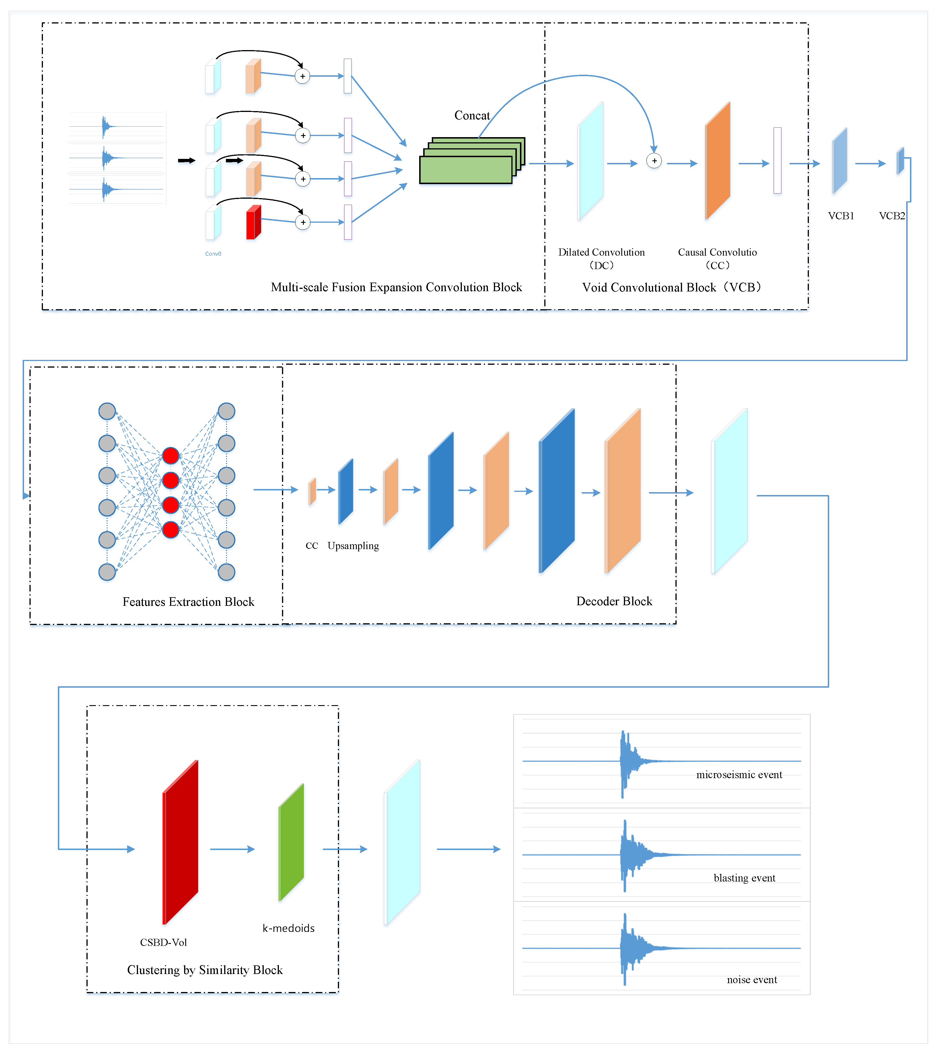
In this model, all convolution layers adopt a one-dimensional design, and the data dimensions processed include the number of variables and the corresponding waveforms. The overall structure of MDCAE is divided into four main parts: multi-scale fusion expanded convolution module, dilated convolution module, feature extraction module, and decoding module. The initial part of the multi-scale fusion expanded convolution module performs data extraction through four standard convolution blocks of convolution kernels of size 1; followed by three expanded convolution blocks using convolution kernels of sizes 3, 5, and 7; and a final maximum pooling layer. The convolution results of the four different scales are processed by the residual block and spectral regularization and then concatenated and output by columns. The dilated convolution module includes a dilated convolution layer, a residual block, a causal convolution layer with a stride of 2, and a spectral regularization layer. The feature extraction module is composed of three fully connected layers, of which the first layer contains 256 neurons, the second layer 50, and the third layer again 256. The features extracted by the second layer are the target features. The decoding module is composed of alternating causal convolution layers and upsampling layers, and finally, the dilated convolution layer is used to reconstruct the data waveform. The detailed network structure diagram is shown in
Figure 1.
The model consists of four main modules: the multi-scale fusion convolution block, the dilated convolution block, the feature extraction module, and the decoder. Each component is specifically designed to extract rich, robust features from microseismic time-series signals. The multi-scale convolution block utilizes kernels of various sizes (1, 3, 5, and 7) to capture both local and global information. The dilated convolution block expands the receptive field without increasing parameters. The feature extraction module compresses the data into a 50-dimensional latent space, which is then decoded to reconstruct the input waveform. Spectral normalization is incorporated in multiple layers to stabilize training and enhance generalization.
4. Similarity Measurement Model and Clustering Model
In the task of time series clustering, existing similarity measurement methods frequently encounter challenges such as the improper alignment of time series or excessive computational complexity, which directly affect the accuracy of the clustering results. Therefore, optimizing the current similarity measurement technology is of importance and practical value. The Shape-Based Distance (SBD) algorithm can more effectively capture the patterns and trends in time series, especially when the amplitudes and baselines of time series may be inconsistent [
41]. The time complexity of the SBD algorithm is
, which is superior in computational efficiency to traditional distance-based measurement methods represented by the Dynamic Time Warping (DTW) algorithm, especially when dealing with longer time series. Therefore, we apply the SBD algorithm to microseismic waveform recognition to improve the recognition speed and clustering effect.
4.1. The Basis of Time Series Clustering
The core task of time series clustering is to group according to the similarity between time series. This process aims to identify and assign similar patterns and trends to different categories. These patterns may include the periodicity, trend, or other features. Clustering algorithms evaluate the distance between time series by applying similarity metrics (such as Euclidean distance or Dynamic Time Warping distance) and accordingly group similar sequences into one category. The challenges faced by time series clustering include dealing with high-dimensional data, where each sequence may contain hundreds to thousands of data points. At the same time, time series are often accompanied by problems of noise and missing values, which need to be properly handled before clustering. Typical clustering algorithms, such as k-means, hierarchical clustering, and DBSCAN, all adopt different strategies to adapt to the characteristics and similarity metrics of time series. In time series clustering, the selection of an appropriate algorithm and distance metric standard is the key [
42,
43].
Time series clustering is usually divided into three major steps: feature extraction, similarity measurement, and the clustering algorithm.
The goal of feature extraction is to transform the original time series into representative and distinguishable features so that machine learning algorithms can handle them more effectively. This step is dedicated to extracting the main information in the time series.
Similarity measurement is crucial in time series analysis. It is responsible for defining and calculating the similarity or distance between sequences and is the cornerstone of many analysis tasks. This module improves the accuracy of the clustering results by comparing different time series and evaluating their similarity.
The goal of the clustering algorithm is to divide a set of time series into clusters so that sequences within the same cluster are highly similar, while sequences between clusters are significantly different. The quality of clustering largely depends on the similarity measurement method adopted.
4.2. SBD Algorithm with Constrained Time Window Fusing Volatility
The application of the SBD algorithm with a constrained time window (CSBD) [
44] in time series clustering analysis aims to improve the clustering accuracy by improving the similarity measurement method. Compared with the traditional SBD algorithm, this algorithm introduces the constrained time window technology to capture the shape similarity of time series more flexibly at different time scales, thereby improving the accuracy and reliability of the clustering results.
Volatility was initially introduced as a concept to measure the fluctuation of financial markets or asset prices and is usually used for the classification of financial time series [
45]. Since vibration data has similar characteristics to financial time series, this paper proposes a method to calculate the volatility of vibration waveform sequences and combines the SBD algorithm to propose the SBD algorithm fusing volatility to improve the classification accuracy.
Our definition of volatility is shown in Equation (2):
Here,
represents the coefficient of variation, which is used to reflect the degree of dispersion of the variable;
represents the kurtosis, which is an indicator used to describe the sharpness or tail thickness of the data distribution;
represents the range of the data; and
represents the interquartile range of the data. The calculation of
and
is as follows:
Here,
represents the variance of the data, and
represents the average value of the data.
Here, E represents the expected value; represents the mean value of the variable.
The core idea of this algorithm is that by defining an appropriate size of the constrained time window, the algorithm can perform local similarity measurement on different parts of the time series and then comprehensively evaluate the overall shape similarity. This method allows the algorithm to capture short-term fluctuations and long-term trends in the time series and provides a more fine-grained similarity comparison method for time series with different characteristics.
During the operation, the original time series data is first preprocessed with data fusing volatility, and then the algorithm is initialized by selecting an appropriate size of the constrained time window. This step is crucial for capturing the key shape features of the time series. Subsequently, the algorithm sets a constrained time window on each time series, calculates the shape similarity of the data within the window, and integrates these local similarity measurements into a global similarity measurement. In this way, the SBD algorithm with a constrained time window can more accurately reflect the similarity between time series.
In the clustering stage, this algorithm uses the calculated global similarity measurement matrix and adopts the k-medoids method to assign time series to each cluster according to the shape similarity. This clustering strategy that combines the constrained time window technology and shape similarity not only improves the flexibility and adaptability of the time series clustering task but also enhances the interpretability and practicality of the clustering results. To ensure the accuracy and reliability of the clustering effect, the algorithm further adopts three indicators, namely the Silhouette Coefficient (SC), the Rand Index (RI), Adjusted Rand Index (ARI), and the Normalized Mutual Information (NMI), to comprehensively evaluate the clustering results. This comprehensive evaluation mechanism ensures the quality of the clustering results, enabling the algorithm to provide more accurate and meaningful clustering solutions when dealing with complex time series data. The CSBD-Vol algorithm is shown in
Algorithm A1. The pseudocode of
Algorithm A1 is provided in
Appendix A.
4.3. Algorithm Structure
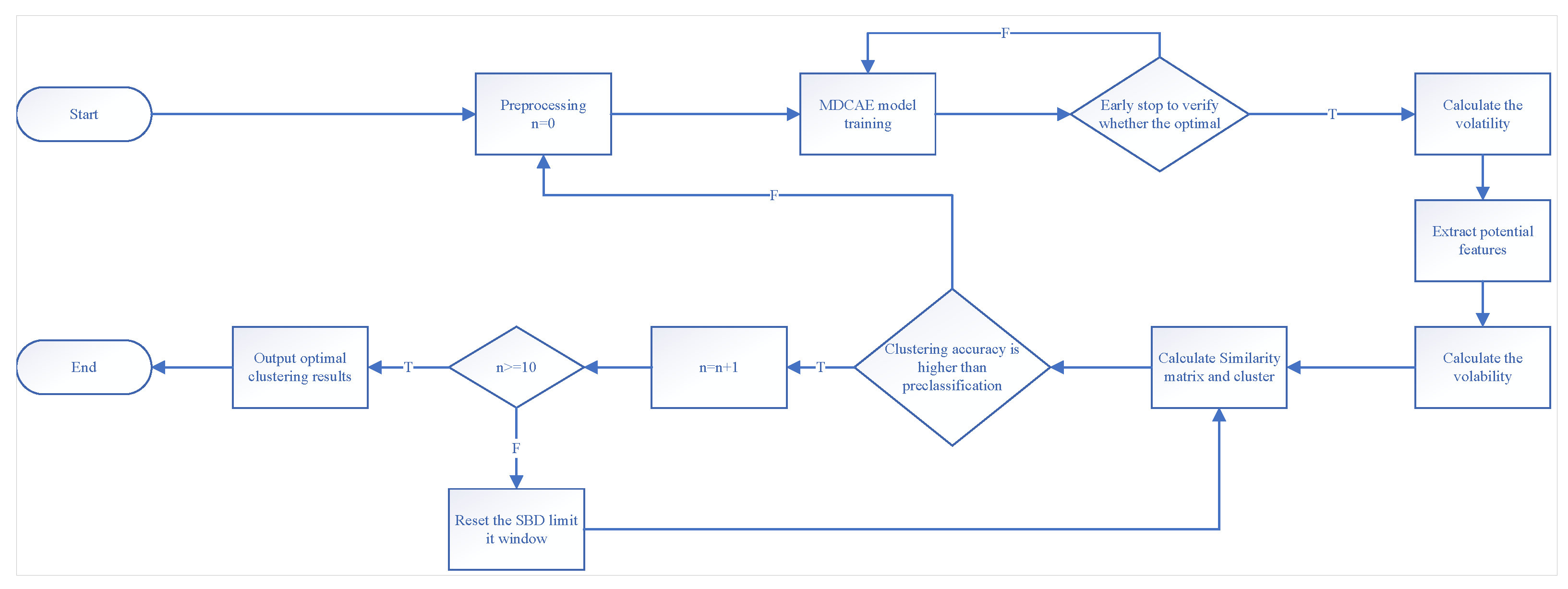
The detailed process of the MDCAE-CSBD-Vol algorithm is shown in
Figure 2.
Firstly, the time series data is input into the system, and the max–min normalization processing of the data is performed to ensure that the data is compared on the same scale. The normalization formula is as follows:
where
represents the maximum value of the time series within this time period, and
represents the minimum value.
Although max–min normalization ensures that different time series are brought to a common scale, it may obscure differences in variance and potentially distort the relative distances between data points. To mitigate this issue, the proposed MDCAE-CSBD-Vol model incorporates several robustness mechanisms. First, the MDCAE architecture leverages multi-scale fusion and dilated convolutions to extract hierarchical features that capture both local fluctuations and global patterns, which are less sensitive to raw value scales. Second, spectral regularization is applied during training to prevent overfitting to particular scale ranges. Finally, in the similarity measurement phase, we introduce a volatility-based distance metric that includes statistical descriptors such as variance, kurtosis, and interquartile range. These enhancements ensure that the model maintains robustness against the limitations of basic normalization and preserves essential shape characteristics of the time series.
After the time series data is input into the system, the combination of the MDCAE model and the CSBD algorithm, after performing the max–min normalization processing of the data, ensures the comparison of different time series on a unified scale. This process covers the calculation of the maximum and minimum values of the data within a specific time period. Then, based on the normalized data, the model is initialized according to the characteristics of the specific time series data, and the appropriate size of the constrained time window and the optimal number of iterations are determined. During the model training stage, the early stopping method is used to determine whether the best model fitting effect is achieved. Specifically, we monitor the changes in four clustering evaluation metrics: Silhouette Coefficient (SC), Rand Index (RI), Adjusted Rand Index (ARI) and Normalized Mutual Information (NMI). If none of these indicators improve significantly within 10 consecutive iterations, the training is terminated early. This prevents overfitting and reduces unnecessary computation.
After the training is completed, the low-dimensional feature vectors extracted by the model are used to perform the initial k-means clustering, and the evaluation index of the clustering effect, such as the Rand Index (RI), is recorded at the same time. At this time, the CSBD algorithm calculates the shape similarity index of each time series based on the extracted feature vectors and constructs the similarity matrix. Using this matrix, the algorithm performs iterative clustering, and dynamically adjusts the size of the constrained time window during the process until the clustering effect no longer improves significantly and then outputs the final clustering result to complete the clustering analysis task of the time series.
5. Experiment
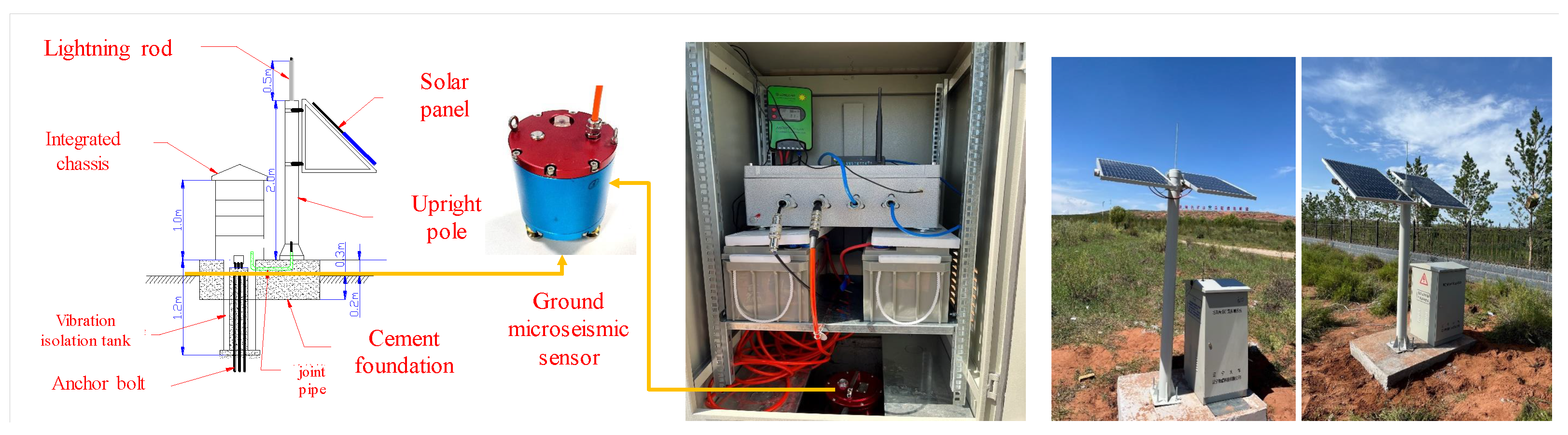
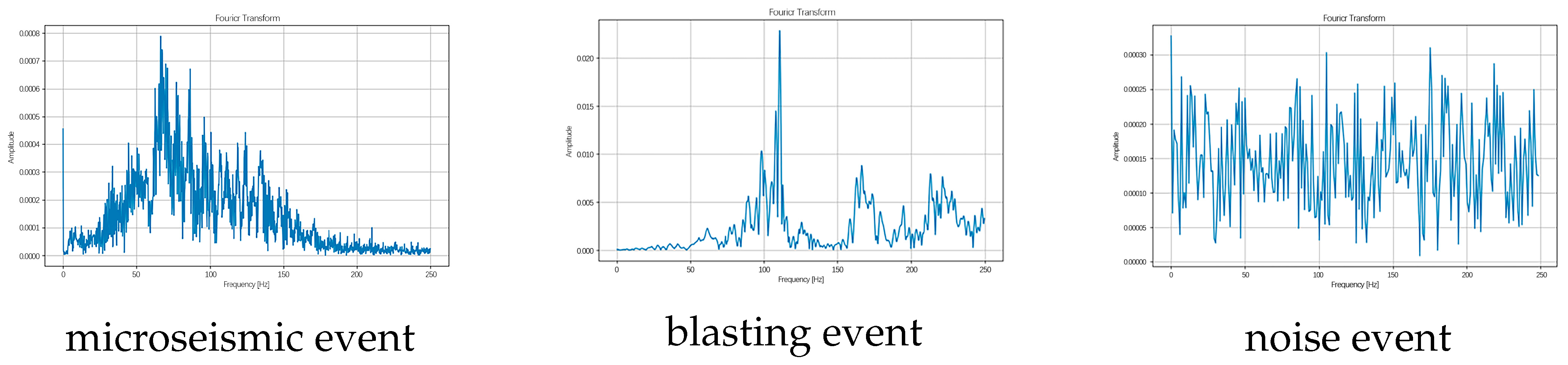
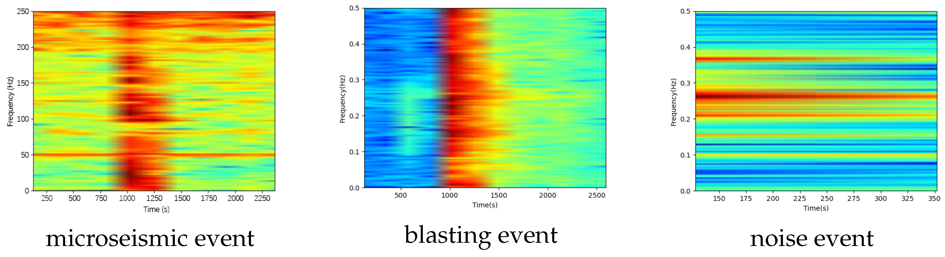
We used the microseismic monitoring data of the 802 working faces in a certain mining area, combined with the experimental dataset of the production cost. The microseismic data was collected by the equipment of the ground microseismic detection station, as shown in
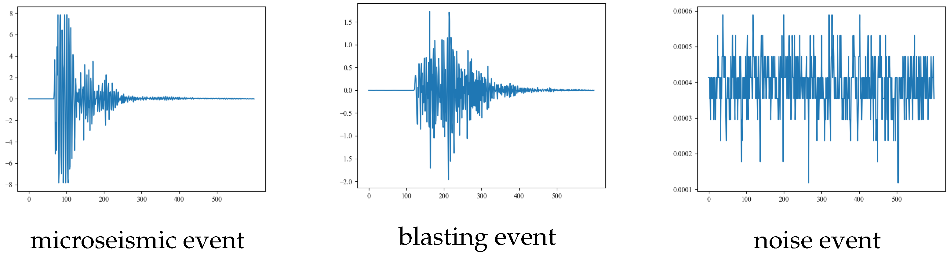
Figure 3 specifically. The sampling frequency of the microseismic monitoring data was 500 Hz. The experimental dataset contains 500 microseismic event waveforms, 500 blasting event waveforms, and 500 non-event waveforms (noise waveforms).
Figure 4 and
Figure 5 show the corresponding waveforms and spectrograms, while the time series diagrams are presented in
Figure 6. The length of each data segment is 600, and the data is normalized by the maximum and minimum values.
5.1. Evaluation Indicator
When evaluating the performance of unsupervised clustering algorithms, key indicators include the Silhouette Coefficient, the Rand Index, the Adjusted Rand Index, and the Normalized Mutual Information.
The Silhouette Coefficient (SC) [
46] can be used to assess the compactness of clustering results. Its value range is between −1 and 1, and a larger value indicates better clustering effects. The calculation formula of the Silhouette Coefficient is as follows:
Here, represents the average distance of other samples within the cluster to which i belongs, and represents the minimum average distance of i to the samples of other clusters.
The Rand Index (RI) provides a method to measure the similarity of clustering results [
47] and is used to evaluate the accuracy of clustering algorithms in data classification tasks. This index is calculated based on the comparison of the number of similar and dissimilar sample pairs within two clustering results. Its value ranges from 0 to 1. A value close to 1 indicates a high degree of consistency in the clustering results, while a value close to 0 indicates significant differences between the two results. When using the Rand Index to evaluate the performance of clustering algorithms in unsupervised learning, it should be noted that the Rand Index may be biased in situations with a large number of categories. Therefore, a comprehensive evaluation should be conducted in combination with other evaluation indicators. In addition, when the Rand Index is applied to cluster analysis with a known label set, it can be used as an indicator to measure the difference between the clustering results and the true labels. The calculation formula of the Rand Index is as follows:
Here, represents the number of samples that are of the same category and are classified in the same cluster, refers to the number of samples of different categories and distributed in different clusters, involves the number of samples of different categories but classified in the same cluster, and refers to the number of samples of the same category but distributed in different clusters.
The Adjusted Rand Index (ARI) optimizes the original Rand Index. The Rand Index does not always remain stable close to zero when dealing with random classification results. Therefore, ARI is introduced to reflect the clustering effect more accurately [
48]. ARI is similar to the Rand Index and is used to assess the consistency of two clustering results. It estimates the similarity by counting the similar or dissimilar sample pairs in the two clustering results and incorporates the consideration of the influence of randomness on clustering. The value of ARI ranges from −1 to 1. The closer the value is to 1, the higher the similarity of the two clustering results; the closer to −1, the greater the difference. When ARI is 0, it means that the clustering results are no different from random assignment. The feature of ARI is that it can eliminate the interference of randomness on clustering judgment and is usually used to evaluate the performance of the clustering algorithm on the actual dataset. The calculation formula of the Adjusted Rand Index is as follows:
Here, is the Rand Index.
The Normalized Mutual Information (NMI) is a measure of the similarity of two clustering results. After applying different clustering algorithms, in order to evaluate the effect of the algorithm or the superiority of parameter configuration, it is often necessary to compare the clustering results [
49]. At this time, the NMI metric can be used to estimate the similarity of the two clustering results. NMI normalizes the mutual information between the two clustering results to generate a value between 0 and 1, which reflects the similarity degree of the two clustering results. The calculation formula of the Normalized Mutual Information is as follows:
Here, represents the mutual information between X and Y, and and represent the entropies of X and Y, respectively. The value range of the Normalized Mutual Information is between 0 and 1, and a larger value indicates greater similarity between the two clustering results.
5.2. Feature Extraction Experiment
To verify the model’s ability to extract and reconstruct features, we conducted the following feature extraction experiment to verify the validity of the model.
We used the vibration waveforms of the 802 working faces in a certain mining area to construct the dataset, with a sampling frequency of 500 Hz. Firstly, the data was preprocessed, and 500 microseismic event waveforms, 500 noise event waveforms, and 500 blasting event waveforms were extracted. These datasets were standardized as the input of the model. The weight initialization of the model adopts variance scaling initialization. This method can adaptively adjust the variance of the initial distribution according to the number of neurons in each layer, alleviate the problems of gradient explosion or gradient disappearance, and improve the training efficiency of the neural network. Compared with the traditional Gaussian distribution initialization and the truncated Gaussian distribution initialization, using variance scaling initialization enables the model to have better generalization ability.
In this model, we used the Adam optimizer, the loss function was set as the mean square error, and the batch size was 128.
Table 1 shows the comparison of the model’s reconstruction performance under different regularization methods.
In this model, using spectral regularization proved to be the best choice, as it outperformed layer normalization and batch normalization in both reconstruction performance and the optimal reconstruction effect after 500 iterations. This confirms that adopting spectral regularization significantly enhances the stability and quality of the reconstruction model.
Subsequently, we conducted a series of ablation experiments to verify the positive impact of various modules on the model’s performance. We compared the model with
MCAE, using multi-scale fusion convolution blocks but not using dilated convolution blocks.
DCAE, using dilated convolution blocks but not using multi-scale fusion convolution blocks.
CAE, an autoencoder that does not use multi-scale fusion convolution blocks or dilated convolution blocks.
For consistency, each model employed variance scaling initialization and spectral regularization as the regularization term, with early stopping set to a patience value of 50 to determine if the optimal solution was reached. The detailed experimental results are presented in
Table 2.
Table 2 summarizes the mean square error (MSE) of all ablation experiment models on the dataset. Compared with other models, the MDCAE model proposed in this paper performs best in the reconstruction effect. For a comprehensive comparison, we compared this model with the ExtraMAE [
50] model, the LSTM-SAE [
51] model, and the Time-VAE [
52] model. The results show that although the optimal number of iterations of our proposed MDCAE model is slightly higher than that of other models, it still performs well in the reconstruction effect.
Table 3 summarizes the MSE scores of all candidate models and the number of iterations to reach the best state.
The ExtraMAE model integrates the concepts of Autoencoder and Matrix Factorization to obtain a compact, low-dimensional representation of time series data and maintain the accuracy of reconstruction.
The basic idea of the LSTM-SAE model is to encode the input sequence through the LSTM layer and then decode and reconstruct it through the reverse LSTM layer. The stacking of multiple LSTM layers helps to learn richer and more advanced sequence features.
The Time-VAE model is a variational autoencoder model for time series data modeling. It is an extension of the standard VAE model specifically designed to handle the features and structures of time series data. By training the Time-VAE model, we can achieve meaningful low-dimensional representation learning of time series data and at the same time have the ability to reconstruct and generate new samples. This latent representation learning can be used in various applications such as data visualization, dimensionality reduction, and anomaly detection.
5.3. Clustering Comparison Experiment
This experiment was conducted on a computer with 11th Gen Intel(R) Core(TM) i7-11700K 3.60 GHz, RAM: 32.0 GB, and graphics card NVIDIA GeForce RTX3050, using python 3.9 and tensorflow-gpu 2.6.0. The data was input into the MDCAE model for training, and then the similarity measurement matrices were extracted using the CSBD-Vol, CSBD, SBD-Vol, and SBD algorithms, respectively, and k-medoids clustering was performed. The results are shown in detail in
Table 4.
From the results presented in
Table 4, it can be seen that the running time cost of the SBD algorithm without adding the constrained time window is higher than that of adding the constrained time window. Moreover, the tail oscillation effect of the time series without adding the constrained time window is extremely sensitive, resulting in a higher classification error rate. Therefore, it can be concluded that for time series clustering, adding a constrained time window is necessary. The volatility proposed in this paper has greatly improved the accuracy and robustness of the algorithm. The CSBD-Vol algorithm, which incorporates volatility and adds a constrained time window, performs excellently in multiple indicators such as the Silhouette Coefficient, the Rand Index, the Adjusted Rand Index, and the standardized mutual information. The final clustering RI reaches more than 87%. This indicates that each component of the algorithm model is indispensable, and they complement each other and play a key role.
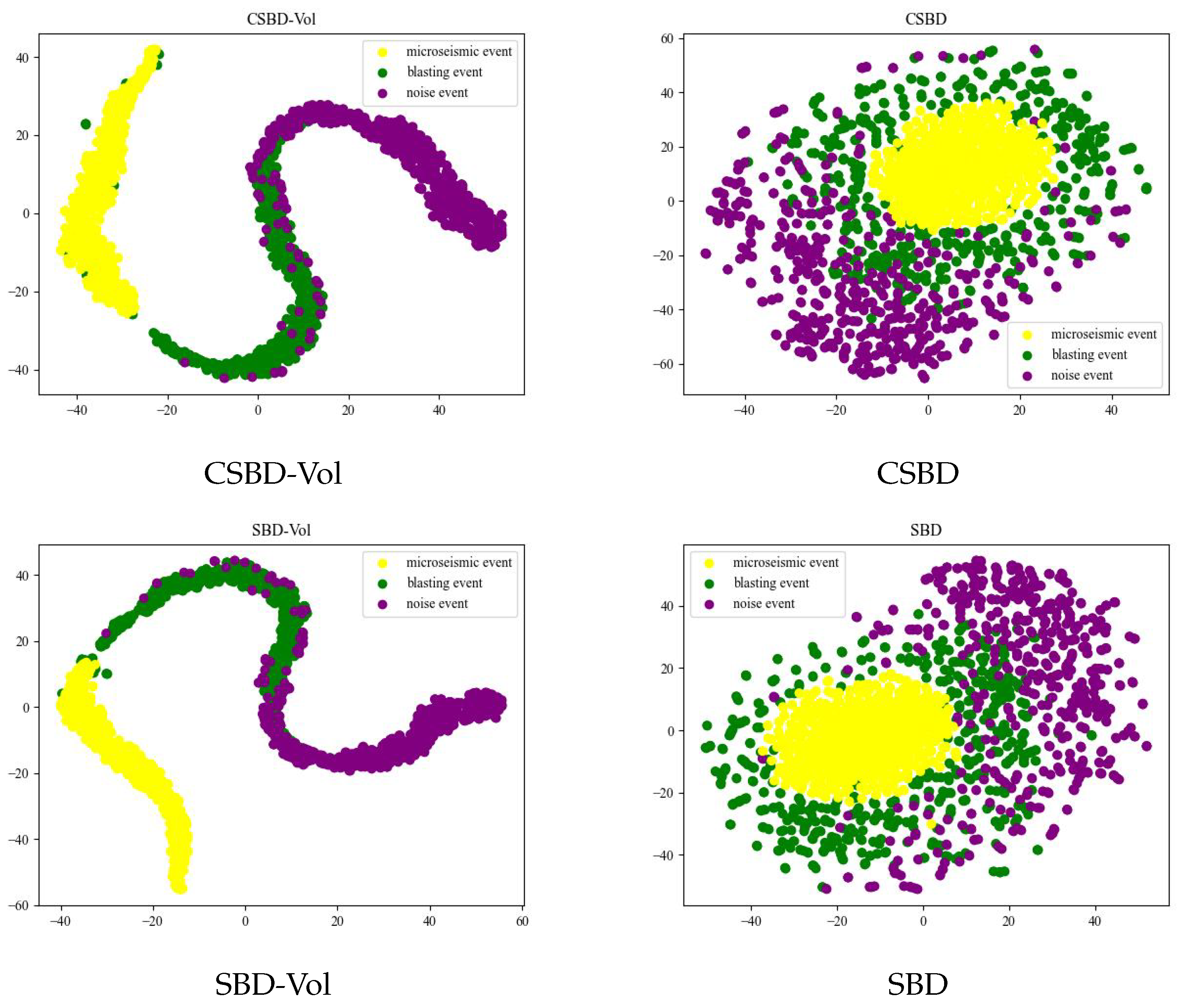
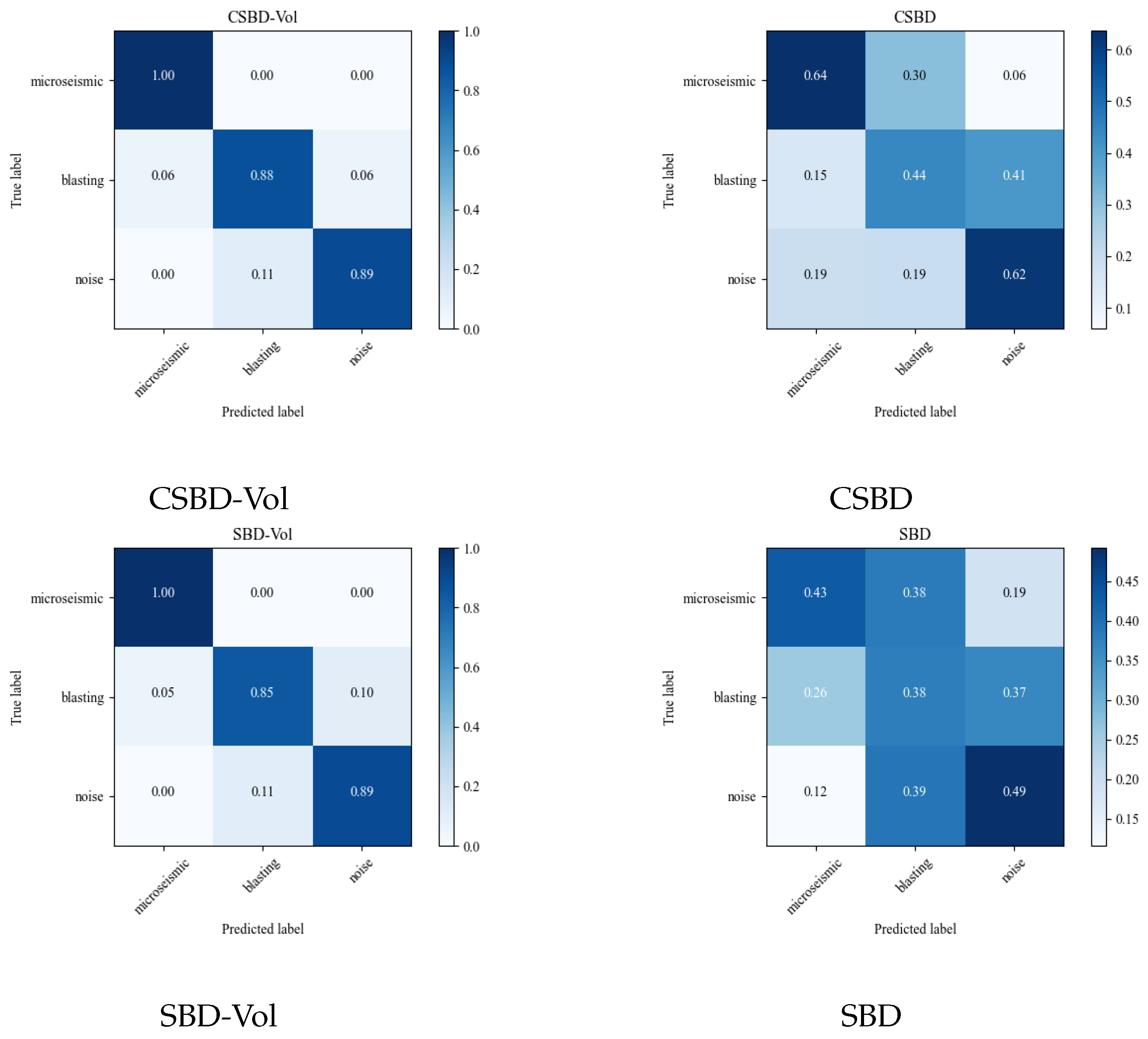
Figure 7 and
Figure 8 present the clustering effects under the four calculation methods of CSBD-Vol, CSBD, SBD-Vol, and SBD, respectively.
According to the results shown in
Figure 7 and
Figure 8, the clustering effect of the CSBD algorithm fused with volatility is significantly better than the original SBD and other algorithms, especially showing significant advantages in the discrimination between microseismic events and other events such as blasting and noise. Therefore, it can be concluded that the CSBD-Vol algorithm proposed in this paper provides a new, more accurate and efficient method for capturing abnormal events in the microseismic system.
6. Conclusions
This paper proposes a k-medoids clustering algorithm that uses MDCAE as the feature extraction module and CSBD as the similarity measurement module and fuses volatility. The main conclusions are as follows.
Despite these promising results, several limitations and delimitations exist. First, the model was primarily validated on microseismic data from a single mining face, which may limit its generalizability across different geological settings. Second, while the proposed volatility metric enhances shape similarity discrimination, it relies on statistical properties that may be sensitive to signal length or preprocessing techniques. Third, we focused solely on unsupervised clustering performance without incorporating domain knowledge or expert labels, which could further refine the results.
Future research should explore multi-source microseismic data integration from different mines to test the robustness and transferability of the model. Additionally, extending the framework to semi-supervised or weakly supervised scenarios could leverage minimal expert labeling to further improve accuracy. Integration with time-series prediction models or real-time event detection systems is also a promising direction.
Scientifically, this work contributes a novel deep clustering architecture that leverages time-window constraints and waveform volatility, which can significantly improve the interpretability and robustness of clustering results. The algorithm enhances waveform characterization and clustering performance in noisy and unlabeled environments, offering a scalable and practical solution for dynamic event monitoring in mining and other geophysical domains.
The MDCAE module shows excellent reconstruction accuracy when dealing with time series problems to improve the feature extraction ability. By introducing strategies such as spectral regularization, multi-scale fusion convolution, and dilated convolution blocks, the MDCAE module overcomes the reconstruction difficulties of the original autoencoder in the face of slight disturbances and solves the balance problem between the number of model parameters and the size of the receptive field. This series of improvements significantly enhances the accuracy of reconstruction.
The Shape-Based Distance (SBD) algorithm shows significant advantages in processing time series data. Firstly, the SBD algorithm optimizes the distance calculation method and can effectively handle the deformation of time series data, which is particularly important in time series data analysis. Secondly, the SBD algorithm optimizes the calculation method of the centroid, making the clustering results more accurate and thereby improving the accuracy of data analysis. In addition, the SBD algorithm supports amplitude scaling and translation invariance, which enables it to better handle the characteristics of time series data and further improves the effect of data analysis.
The CSBD algorithm solves the problem of the excessively high time complexity of traditional distance-based measurement methods represented by the Dynamic Time Warping (DTW) algorithm and introduces a constrained time window to further reduce the time complexity of the algorithm.
The CSBD-Vol algorithm is proposed to solve the problem that the traditional SBD algorithm is easily disturbed by noise. This algorithm introduces a restricted window, thereby reducing the time complexity, and borrows the concept of volatility from the financial field and integrates the redefined volatility formula into the algorithm, thereby solving the problem that the traditional algorithm is sensitive to noise.
The MDCAE-CSBD-Vol algorithm makes full use of the features extracted by MDCAE to measure similarity, thereby improving the clustering efficiency of the model.
To sum up, the MDCAE-CSBD-Vol algorithm belongs to the unsupervised clustering algorithm, eliminating the dependence of traditional deep learning algorithms on labels. It only uses unlabeled data for unsupervised learning and achieves excellent clustering results, providing a new method for the field of microseismic pattern recognition.


