An Algorithm for Mining Frequent Approximate Subgraphs with Structural and Label Variations in Graph Collections

Abstract

Using graphs as a data structure is a simple way to represent relationships between objects. Consequently, it has raised the need for algorithms to process, analyze, and extract meaningful information from graphs. Therefore, frequent subgraph mining (FSM) algorithms have been reported in the literature to discover interesting, unexpected, and useful patterns in graph databases. Frequent subgraph mining involves discovering subgraphs that appear no less than a user-specified threshold; this can be performed exactly or approximately. Although several algorithms for mining frequent approximate subgraphs exist, mining this type of subgraph in graph collections has scarcely been addressed. Thus, we propose AGCM-SLV, an algorithm for mining frequent approximate subgraphs within a graph collection that allows structural and label variations. Unlike other FSM approaches, our proposed algorithm tracks subgraph occurrences and their structural dissimilarities, allowing user-defined partial similarities between node and edge labels, and captures frequent approximate subgraphs (patterns) that would otherwise be overlooked. Experiments on real-world datasets demonstrate that our algorithm identifies more patterns than the most similar state-of-the-art algorithm with a shorter runtime. We also present experiments in which we add white noise to the graph collection at different levels, revealing that over 99% of the patterns extracted without noise are preserved under noisy conditions, making the proposed algorithm noise-tolerant.

1. Introduction

In several areas, such as government, industry, and science, knowledge derived from data is of great importance. Therefore, it is important to develop methods for extracting useful information and knowledge [1,2,3,4]. This problem is studied in pattern mining, a data mining technique that aims to discover interesting, unexpected, and useful patterns [5].

A trend in pattern mining is the development of algorithms designed to analyze complex data such as graphs [6,7]. Graphs have become popular due to their flexibility and simplicity in representing relationships between objects [8,9] and are widely used in science and technology to describe and visualize data [10]. These characteristics have led to the use of graphs in many applications, such as medicine [11,12], chemistry [13,14], bioinformatics [15,16], social networks [17,18,19], linguistics [20,21], computer vision [22,23,24], and image classification [25,26], among others. Despite their advantages, data mining algorithms for pattern mining cannot be directly applied to graphs due to their complex structure. Consequently, it is necessary to develop algorithms capable of mining patterns in graphs [27]. Mining patterns in graphs refers to the mining of frequent subgraphs in a single graph or graph collection.

Frequent subgraph mining (FSM) involves discovering subgraphs that repeat no less than a user-specified threshold [28,29,30] in a single graph or graph collection. FSM can be performed exactly or approximately. Frequent exact subgraph mining aims to mine subgraphs with one-to-one correspondence (isomorphism). Several algorithms have been developed to mine exact frequent subgraphs [31,32,33,34,35,36,37,38,39,40]. In contrast, frequent approximate subgraph mining aims to mine subgraphs allowing variations in their structure or labels. Therefore, approximate FSM allows dealing with distortions found in real-world applications, such as noisy data, data diversity, and uncertain data [41,42,43].

However, despite its usefulness in real-world applications, approximate FSM introduces significant computational challenges. The problem is inherently more complex than frequent exact subgraph mining, as it requires approximate matching techniques that are more computationally expensive.

Although approximate FSM has already addressed structural variations, most algorithms reported in the literature address frequent approximate subgraph mining with structural variations in a single graph [44,45,46]. While the literature mentions that the algorithms for mining subgraphs in a single graph can be extended to mine subgraphs in graph collections [47], it is not an easy task because subgraphs obtained by an algorithm for a single graph differ from those obtained by an algorithm for a graph collection.

The literature describes only one algorithm, REAFUM [48], for mining frequent approximate subgraphs in an undirected graph collection. This algorithm can handle structural and label variations in edges and nodes. Nevertheless, it mines the subgraphs from a small subset of representative graphs in the collection. Therefore, this paper addresses the problem of mining all frequent approximate subgraphs in graph collections, allowing structural and label variations in nodes and edges.

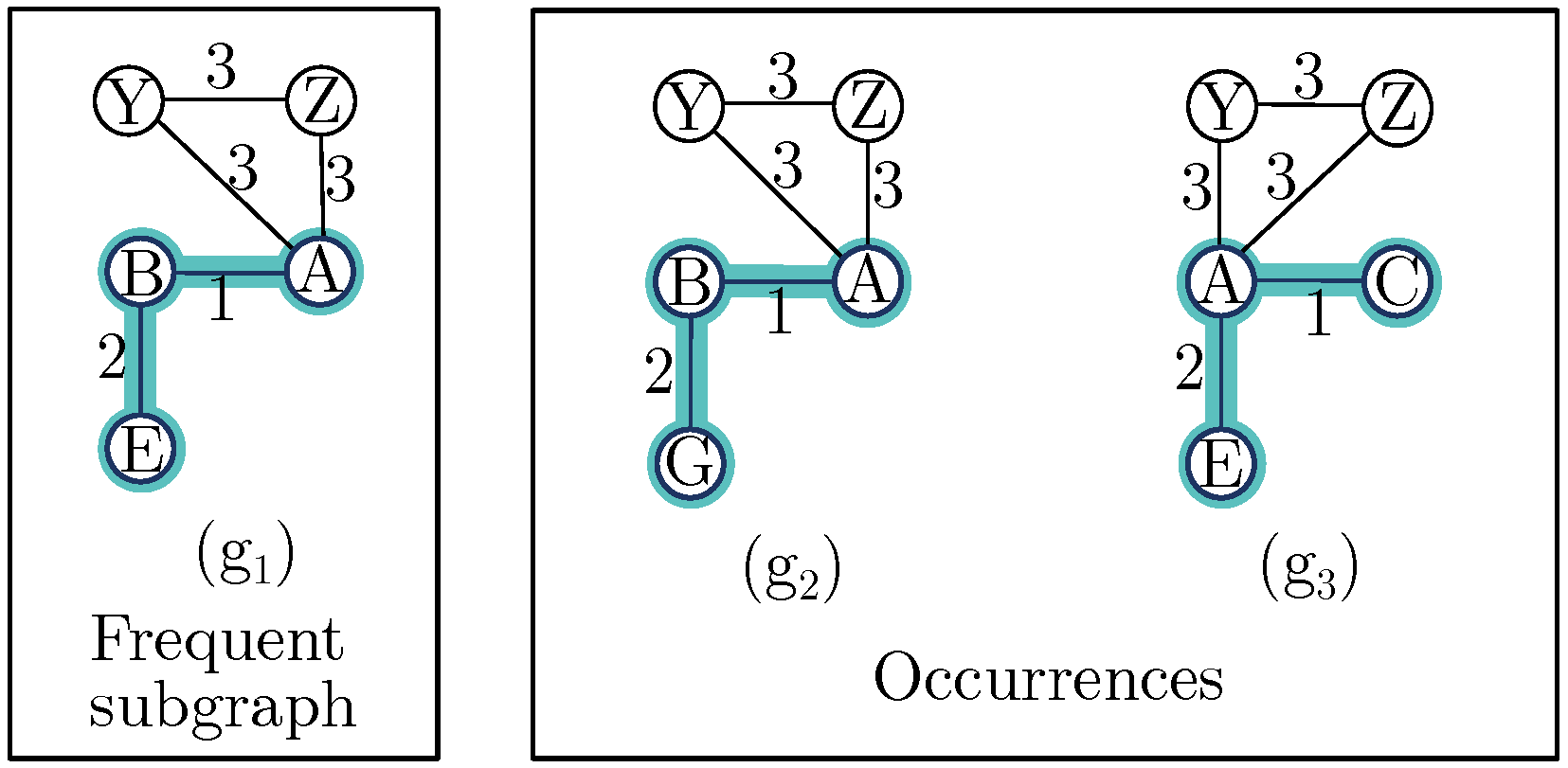
The contribution of this paper is the AGCM-SLV (Approximate Graph Collection Miner with Structural and Label Variations) algorithm (see Section 4), which is designed to mine all frequent approximate subgraphs within an undirected labeled graph collection, allowing variations in both node and edge labels as well as in the structure of the graphs. For handling label variations, the proposed algorithm allows defining partial similarities between the labels of nodes and edges. For handling structural variations, AGCM-SLV stores all the occurrences of a frequent subgraph and its corresponding dissimilarity.

Experiments on real-world datasets reveal that the proposed algorithm mines more frequent approximate subgraphs with structural and label variations in a lower runtime than REAFUM [48], the most similar state-of-the-art algorithm.

This paper is organized as follows: In Section 2, the related work is presented. Section 3 provides some basic concepts. Section 4 introduces the proposed algorithm AGCM-SLV (Approximate Graph Collection Miner with Structural and Label Variations) for mining frequent approximate subgraphs in graph collections that exhibit structural and label variations. In Section 5, the experimental results are shown and discussed. Finally, we provide our conclusions in Section 6.

2. Related Work

In this section, we discuss the previous works most related to ours. Specifically, we focus on frequent approximate subgraph mining algorithms. Frequent approximate subgraph mining has been approached in a single graph or a graph collection.

2.1. Frequent Approximate Subgraphs in a Single Graph

Graph mining algorithms reported in the literature have addressed three problems in a single graph: only structural variations, only label variations, and a combination of label and structural variations.

Algorithms such as SUBDUE [49], SUBDUECL [50], GREW [51], the proposed algorithm in [52], and Ap-FSM [53] address structural variations in a single graph. SUBDUE is based on compressing parts of the graph using node contraction into a single node. Each compression is a frequent segment within the graph, preserving the best ones. SUBDUECL improves the selection of frequent subgraphs when compressing by counting positive and negative examples. GREW is a heuristic algorithm that mines frequent subgraphs from a large graph; it uses edge contraction, compressing frequent subgraphs into new nodes. In [52], an approximate graph matching algorithm that uses node contraction in smaller degree nodes in a single graph is introduced. Another approach is followed by Ap-FSM [53], which mines frequent subgraphs from a single large graph using the distributed framework Pregel. This algorithm selects representative graphs through a sampling technique from the original large graph and focuses on mining frequent subgraphs that are structurally similar to the selected graphs.

In contrast, gApprox [44] introduces variations in nodes labels through a list of similar labels and also incorporates structural variations in edges. The algorithm gApprox uses a variation of edit distance, and to avoid analyzing the subgraph more than once, it introduces a traversal without redundancies. Label variations in a single large graph are also considered by [54], where a cost matrix between the labels is introduced.

Algorithms such as AGrAP [45], MaxAFG [55], the proposed algorithm in [56], and MFP [46] have explored label and structural variations. AGrAP mines all frequent subgraphs into a single undirected labeled graph, allowing label and structure variations in nodes and edges. It also uses a variation of the graph edit distance and traverses the graph using a depth-first search. MaxAFG is an extension of AGRAP; this algorithm mines only maximal frequent subgraphs. The proposed algorithm in [56] introduces a hybrid structural–semantic graph mining approach to mine frequent subgraphs with structural variations based on graph edit distance and semantic node variations in an uncertain graph based on the probability of the presence of an edge. MFP performs frequent subgraph mining, allowing label and structure variation on a single labeled directed graph.

TIPTAP [57] shows the applicability of the structural variations when dealing with an evolving graph, a graph whose structure changes over time. The variations allowed by TIPTAP are based on the insertion and deletion of edges.

2.2. Frequent Approximate Subgraphs in a Graph Collection

Graph mining algorithms reported in the literature have addressed three problems in a graph collection: only structural variations, only label variations, and a combination of label and structural variations.

RAM [58] and UMFGAMW [59] algorithms address structural variations in a graph collection. RAM allows for structural variations in the edges by allowing their absence. It does not allow label variations, and it does not allow structural variations in the nodes. It does not mine all the frequent subgraphs because it performs a random selection of candidates, eliminating those with similar characteristics to candidates that have already been analyzed. UMFGAMW [59] mines uncertain maximal frequent subgraphs in a graph collection. Due to the nature of uncertain graphs, it mines approximate subgraphs with a similar structure based on the probability of an edge’s presence.

APGM [42], and VEAM [41] have addressed label variation. APGM mines clique frequent subgraphs by representing the graph using a canonical adjacency matrix (CAM). To handle the label variations, it uses a node probability substitution matrix. VEAM mines all frequent subgraphs with label variations in nodes and edges. It uses two probability substitution matrices.

Algorithms such as AMgMiner [60], MgVEAM [61], and CliqueAMgMiner [62] have been reported in the literature for frequent subgraph mining in a graph collection of multigraphs with label variations. AMgMiner preprocesses the multigraphs to convert them into canonical adjacency matrix codes. It occupies two probability substitution matrices to allow for label variations in nodes and edges. MgVEAM, unlike the previous one, introduces a method to mine multigraphs without prior preprocessing by creating a canonical adjacency matrix code that takes multigraphs into account. CliqueAMgMiner mines the clique subgraphs of a multigraph collection.

Regarding label and structural variations in a graph collection, the REAFUM [48] framework allows label and structural variations in nodes and edges. It consists of three stages: selection of representative graphs, expansion of the frequent nodes in search of approximate frequent subgraphs, taking into account the variations in label and structure, and finally, a consensual refinement. To the best of our knowledge, REAFUM is the only algorithm reported in the literature for mining frequent subgraphs in a graph collection. It allows label and structural variations in nodes and edges. However, it does not mine all the frequent subgraphs in a collection; instead, it mines them just from a subset of representative subgraphs, nor does it allow partial similarity in labels.

Table 1. Characteristics of frequent approximate subgraphs algorithms.

Algorithm	Label Variations	Structural Variations
For single graph
SUBDUE (1994)	N/A	Node contraction
gApprox (2007)	Nodes	Edges
AGraP (2014)	Nodes and edges	Nodes and edges
MaxAFG (2014)	Nodes and edges	Nodes and edges
Ap-FSM (2018)	N/A	Based on edge uncertainty
MFP (2021)	Nodes and edges	Nodes and edges
TIPTAP (2021)	N/A	Based on edge variation
For graph collection
RAM (2008)	N/A	Edges
APGM (2010)	Nodes	N/A
VEAM (2012)	Nodes and edges	N/A
REAFUM (2015)	Nodes and edges	Nodes and edges
AMGMiner (2016)	Nodes and edges	N/A
MgVEAM (2017)	Nodes and edges	N/A
UMFGAMW (2018)	N/A	Based on edge uncertainty
CliqueAMGMiner (2020)	Nodes and edges	N/A
Proposed AGCM-SLV	Nodes and edges	Nodes and edges

shows that allowing structural variations for mining frequent approximate subgraphs in graph collections has been scarcely studied. This problem has been explored a bit more for mining frequent approximate subgraphs in a single graph, with a few options reported in the literature. Even though there is an algorithm called REAFUM reported in the literature for mining frequent subgraphs in graph collections considering label and structural variations, it does not mine all frequent approximate subgraphs; it only mines some representative frequent subgraphs. To the best of our knowledge, no algorithm can mine all frequent approximate subgraphs in a graph collection considering both structural and label variations. Therefore, as shown in Table 1, we propose AGCM-SLV.

3. Notation and Preliminaries

This section introduces the notation and definitions used throughout the paper. First, we define an undirected labeled simple graph, since it is the type of graph the graph collection contains.

Definition 1

(Undirected labeled simple graph). An undirected labeled simple graph G is a five-tuple $G=\{N,E,L,\mu ,\varphi \}$, where $N\ne \varnothing$ is the set of nodes, $E\subset N\times N$ is the set of undirected edges, L is the set of labels for nodes and edges, μ is the node labeling function $\mu :N\to L$ that assigns to every node in N a label from L, and $\varphi$ is the edge labeling function $\varphi :E\to L$ that assigns to every edge in E a label from L.

From now on, whenever the term graph is used, it will refer to an undirected labeled simple graph.

Next, we define graph collection, i.e.,  the dataset on which the proposed algorithm performs the mining process.

Definition 2

(Graph collection). A graph collection D is a set of n graphs denoted by $D=\{G_1,G_2,\dots ,G_n\}$.

We also define a subgraph since the proposed algorithm mines frequent approximate subgraphs in a graph collection.

Definition 3

(Subgraph). Let $G=\{N,E,L,\mu ,\varphi \}$ and $G^{\prime }=\{N^{\prime },E^{\prime },L^{\prime },{\mu }^{\prime },{\varphi }^{\prime }\}$ be two undirected labeled simple graphs. $G^{\prime }$ is a subgraph of G denoted by $G^{\prime }\subseteq G$ if the following conditions are accomplished: $N^{\prime }\subseteq N$, i.e., the nodes of $G^{\prime }$ are a subset of the nodes of G, and $E^{\prime }\subseteq E$, i.e., the edges of $G^{\prime }$ are a subset of the edges of G, $\forall u\in V^{\prime }:{\mu }^{\prime }\left(u\right)=\mu \left(f\left(u\right)\right)$ such that ${\mu }^{\prime }\left(u\right)\in L^{\prime }$ and $\mu \left(f\right(u\left)\right)\in L$, $\forall (u,v)\in E^{\prime }:(f\left(u\right),f\left(v\right))\in E$, and ${\varphi }^{\prime }(u,v)=\varphi (f\left(u\right),f\left(v\right))$ such that ${\varphi }^{\prime }(u,v)\in L^{\prime }$ and $\varphi \left(f\right(u),f(v\left)\right)\in L$.

An important part of frequent approximate subgraph mining is determining the similarity between graphs. Therefore, a graph similarity measure is required to determine how similar the subgraphs can be. The dissimilarity function used is based on the graph edit distance [63], which consists of counting the operations required to transform one graph into another.

Definition 4

(Dissimilarity function). Let $G_1=(N_1,E_1,L_1,{\mu }_1,{\varphi }_1)$ and $G_2=(N_2,E_2,L_2,{\mu }_2,{\varphi }_2)$ be two graphs, γ be a node label similarity, and δ be an edge label similarity. The dissimilarity function to be used in the proposed algorithm is the sum of all the costs required to transform a graph $G_1$ into a graph $G_2$. Therefore, the dissimilarity of transforming $G_1$ to $G_2$ is given by:

$$dissimilarity(G_1,G_2)=\sum _{i=1}^{k}C{N}_i+\sum _{j=1}^{m}C{E}_j$$

(1)

where $C{N}_i$ represents the sum of the k modification costs for the nodes, and $C{E}_j$ represents the sum of the m modification costs for the edges. (Note: Depending on the specific structure of the graphs, the node modification cost k or the edge modification cost m can be zero.)

The possible modification costs are:

• Substitution of labels on a node or an edge.

• The node label substitution cost is $1-\gamma ({\nu }_1,{\nu }_2)$, where $\gamma ({\nu }_1,{\nu }_2)\in [0,1]$ represents the similarity between the label of the node ${\nu }_1$ and the label of the node ${\nu }_2$.
• The edge label substitution cost is $1-\delta ({ϵ}_1,{ϵ}_2)$, where $\delta ({ϵ}_1,{ϵ}_2)\in [0,1]$ represents the similarity between the label of the edge ${ϵ}_1$ and the label of the edge ${ϵ}_2$.

• Insertion of a node or an edge.

• The node insertion cost of inserting a ${\nu }_1$-labeled node is 1.
• The edge insertion cost of inserting an ${ϵ}_1$-labeled edge is 1.

• Deletion of a node or an edge.

• The node deletion cost of deleting a ${\nu }_2$-labeled node is 1.
• The edge deletion cost of deleting an ${ϵ}_2$-labeled edge is 1.

Since the proposed algorithm performs frequent approximate subgraph mining, it must be defined when a subgraph is considered frequent. To establish this, we introduce the following definitions.

First, we consider whether a subgraph allowing label and structural variations appears in a graph collection. If it appears, each appearance is viewed as an occurrence of the subgraph:

Definition 5

(Occurrence). Let $D=\{G_1,G_2,\dots G_n\}$ be a graph collection of n undirected labeled simple graphs, $G^{\prime }$ be a subgraph, β be a dissimilarity threshold, and $dissimilarity(G_i,G_j)$ be the graph dissimilarity function described in Definition 4. Then $G^{″}$, a subgraph of $G_i\in D$, is an occurrence of $G^{\prime }$ if $dissimilarity(G^{\prime },G^{″})\le \beta$.

Next, we define the support of a subgraph, which counts the number of graphs in the collection in which the subgraph has at least one occurrence:

Definition 6

(Support). Let $D=\{G_1,G_2,\dots G_n\}$ be a graph collection of n undirected labeled simple graphs and β a dissimilarity threshold. The support of a subgraph $G^{\prime }$ in D, denoted as $Support(G^{\prime },D)$, is defined as:

$$Support(G^{\prime },D)=\frac{{\sum }_{j=1}^{n}f(G^{\prime },G_j)}{\left|D\right|}$$

(2)

where,

$$f(G^{\prime },G_j)=\left\{\begin{array}{cc}1\hfill & \mathit{if}\exists G^{″}\mathit{subgraph}\mathit{of}{G}_j\mathit{such}\mathit{that}{G}^{″}\mathit{is}\mathit{an}\mathit{occurrence}\mathit{of}{G}^{\prime }\mathit{in}{G}_j\hfill \\ 0\hfill & otherwise\hfill \end{array}\right.$$

(3)

Before defining a frequent subgraph, we first define a frequent node, which is the simplest form of a frequent subgraph, consisting of a single node:

Definition 7

(Frequent node). Let $D=\{G_1,G_2,\dots G_n\}$ be a graph collection of n undirected labeled simple graphs and α be a support threshold. A node ν is said to be frequent in the graph collection D if the number of graphs in which it appears, divided by the number of graphs in the collection, is greater than or equal to the support threshold α.

Finally, we define frequent subgraph:

Definition 8

(Frequent subgraph). Let $D=\{G_1,G_2,\dots G_n\}$ be a graph collection of n undirected labeled simple graphs, α a support threshold, and β a dissimilarity threshold. A subgraph $G^{\prime }$ is considered frequent within the graph collection D if there exists at least one frequent node ${\nu }_f$, according to α (see Definition 7), such that for each occurrence $G^{″}$ of $G^{\prime }$, according to β (see Definition 5), ${\nu }_f\in V_{G^{″}}$, and $Support(G^{\prime },D)\ge \alpha$.

Another important aspect to consider is to reduce the search space and speed up the mining process. For this purpose, we use the anti-monotonicity property, which is defined as follows:

Definition 9

(Anti-monotonicity property). Let D be a graph collection of n undirected labeled simple graphs, and $G^{\prime }$ and $G^{″}$ be two graphs in the graph collection D. If $G^{″}$ is a subgraph of $G^{\prime }$ then $Support(G^{″},D)\ge Support(G^{\prime },D)$.

The anti-monotonicity property states that if a subgraph is not frequent, then none of its supergraphs is frequent; thus, they can be pruned without affecting the search.

4. Proposed Algorithm

This section presents the proposed algorithm for mining all frequent approximate subgraphs with structural and label variations in nodes and edges in a graph collection, named AGCM-SLV (Approximate Graph Collection Miner with Structural and Label Variations).

AGCM-SLV works as follows: First, the algorithm mines all frequent nodes to obtain a set of frequent subgraphs containing a single node. After that, a subgraph expansion process begins, where frequent subgraphs are expanded into larger candidate subgraphs by connecting neighboring nodes and adjacent edges according to a depth-first traversal strategy. Each expansion (candidate subgraph) is verified to determine if it satisfies both the frequency and dissimilarity thresholds. Otherwise, the candidate subgraph cannot be expanded further and must be pruned (discarded) due to the anti-monotonicity property. The expansion process continues until there are no more frequent subgraphs to expand.

Each frequent subgraph mined P is associated with its occurrences in the graph collection, which determines the subgraph’s frequency. These occurrences can have structural and label variations in both nodes and edges. Label variation results from substituting node or edge labels, while structural variations result from representing additional or missing nodes and edges in the frequent subgraph. Because of these variations in labels and structure, each occurrence has a dissimilarity value with the frequent approximate subgraph it represents. This dissimilarity cannot exceed a predefined dissimilarity threshold ($\beta$). The pseudocode for the proposed algorithm is shown in Algorithm 1.

Algorithm 1 Proposed algorithm: AGCM-SLV

Require:  D: graph collection, $\alpha$: support threshold, $\beta$: dissimilarity threshold, $\gamma$: node dictionary (optional), $\delta$: edge dictionary (optional) Ensure:  FS: all unique FREQUENT_SUBGRAPHS    1: $P\leftarrow$ Obtain all FREQUENT_NODES in the graph collection D    2: for every $subgraph$ $G^{\prime }$ in P do    3:       candidate_subgraphs_list ←EXPAND_FREQUENT_SUBGRAPHS($G^{\prime }$)    4:       for every candidate_subgraphs in candidate_subgraphs_list do    5:              for every occurrence o of $G^{\prime }$ do    6:                     expanded_occurrence ←EXPAND_OCCURRENCE(o)    7:                     if dissimilarity(expanded_occurrence, candidate_subgraphs) ≤ β then    8:                           expanded_occurrence is an occurrence of candidate_subgraphs    9:              if Support(candidate_subgraphs,D) ≥ $\alpha$ then  10:                     if candidate_subgraphs has not been mined then  11:                           insert candidate_subgraphs into P and into FS

4.1. Frequent Nodes

In the first stage, all frequent subgraphs formed by a single node are mined by searching through all nodes in the entire graph collection to find those that fulfill the predefined support threshold. These frequent subgraphs, consisting of a single node, are known as frequent nodes (see Definition 7) and are the first set of frequent candidate subgraphs.

4.2. Expand Frequent Subgraph

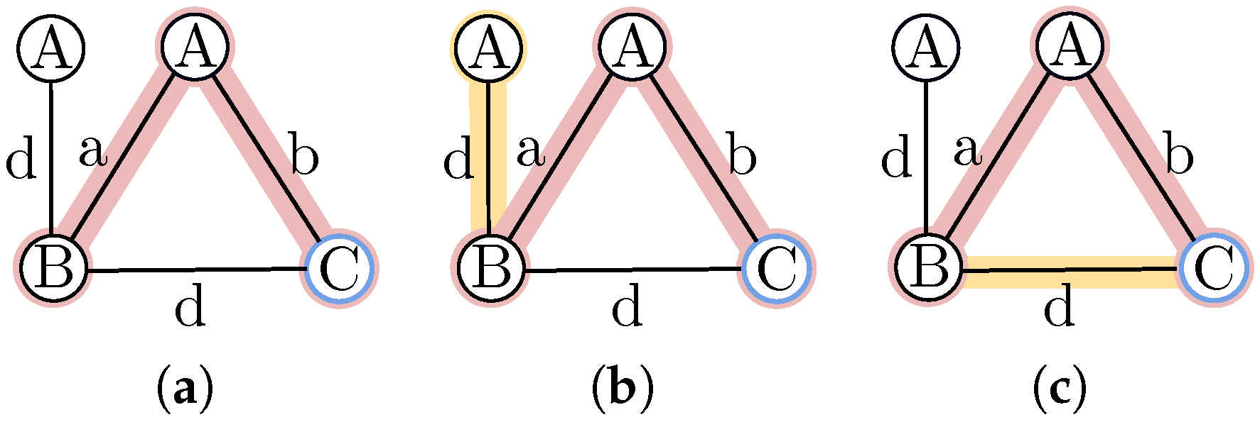
The next step in the proposed algorithm is to expand the current mined frequent subgraphs to obtain new, larger candidate subgraphs. This is achieved by joining each frequent subgraph with one of its neighbor nodes through an edge or by adding an edge in case there is a cycle. This expansion is carried out for every neighbor node or every adjacent edge of the frequent subgraph. Figure 1 shows how a frequent subgraph can be expanded.

4.3. Expand Occurrences

After the candidate subgraphs are generated, the process of identifying their corresponding occurrences within the graph collection begins. To do this, each occurrence of the frequent subgraph that originated the candidate subgraph is expanded.

To explain the expansion process in detail, the following considerations must be established:

• If the node dictionary $\left(\gamma \right)$ or edge dictionary $\left(\delta \right)$, or both, are included, they must be considered when evaluating similarities between labels. Figure 2 illustrates the structure of these dictionaries, each composed of three elements (origin label, similar label, and similarity percentage). In the node dictionary, the node label ‘A’ has a 90% similarity to label ‘B’, while in the edge dictionary, the edge label ‘A’ has a 100% similarity to the edge label ‘B’. It is important to note that the dictionaries’ similarities do not apply in both directions; for example, in the node dictionary, label ‘A’ has a 90% similarity to label ‘B’, but this does not imply that label ‘B’ has a 90% similarity to label ‘A’.
• The new node, ${\nu }_{new}$, is the last node added to a frequent subgraph to form a candidate subgraph.
• A node in a subgraph may have a corresponding node (not necessarily with the same label) in the occurrence, which we will call a mapped node. Since the nodes differ, the maximum allowable dissimilarity must be controlled.
• Not all nodes in the occurrence need to be mapped to nodes in the subgraph. Nodes that are not mapped are called extra nodes.

Before expanding the occurrence $o_{curr}$, it must be verified whether, without modifying it, it fulfills the dissimilarity threshold. Figure 3b shows an example where the occurrence does not expand but is considered a candidate occurrence.

To expand each occurrence $o_{curr}$ of the frequent subgraph that originated the candidate subgraph, the first step is to search for all possible nodes for expansion within the graph containing $o_{curr}$. Each potential expansion node ${\nu }_{exp}$ must be similar to ${\nu }_{new}$. The extra nodes within $o_{curr}$ are also considered in the search. If the $\beta$-occurrence $o_{curr}$ and the candidate subgraph belong to the same graph, the nodes of the candidate subgraph are not considered in the search. From this, there are three possibilities:

• If ${\nu }_{exp}$ is a neighbor of the occurrence $o_{curr}$, a new candidate occurrence $o_{new}$ is created, joining the occurrence $o_{curr}$ with the node ${\nu }_{exp}$, and ${\nu }_{exp}$ is mapped to ${\nu }_{new}$. Figure 3c shows an example of this case, where, ${\nu }_{exp} =$ $\overline{)\mathrm{C}}$ is a neighbor of the occurrence $\overline{)\mathrm{B}}\frac{\mathrm{a}}{}\overline{)\mathrm{A}}$.
• If ${\nu }_{exp}$ is already in the occurrence $o_{curr}$ as an extra node, a new candidate occurrence $o_{new}$ is created, which stays the same as $o_{curr}$, but in it, ${\nu }_{exp}$ is mapped to ${\nu }_{new}$. Figure 3d shows an example where ${\nu }_{exp} =$ $\overline{)\mathrm{C}}$ is already in the occurrence but it was not mapped. $\overline{)\mathrm{C}}$ was an extra node of the $o_{new}$ in $o_{curr}$.
• If, on the other hand, ${\nu }_{new}$ is in the graph of $o_{curr}$ but a path must be created to connect ${\nu }_{exp}$ with $o_{curr}$, the shortest paths connecting ${\nu }_{exp}$ to each node of $o_{curr}$ are searched for. If one path includes another, only the shortest path is considered. For each different path found, a new candidate occurrence $o_{new}$ is created by joining the nodes of the occurrence $o_{curr}$ with the nodes and edges of the path. The intermediate nodes of the path are marked as extra nodes, and ${\nu }_{exp}$ is mapped to ${\nu }_{new}$. Figure 3e shows an example where a path is required to connect ${\nu }_{exp}=$ $\overline{)\mathrm{C}}$. The path with $\frac{\mathrm{d}}{}$ $\overline{)\mathrm{Y}}$ $\frac{\mathrm{b}}{}$ is formed to reach $\overline{)\mathrm{C}}$.

Each occurrence $o_{curr}$ can be expanded through its neighboring edges. If ${ϵ}_{new}$ is a neighbor of the occurrence $o_{curr}$ a new candidate occurrence $o_{new}$ is created, joining $o_{curr}$ with the edge ${ϵ}_{new}$. Figure 3f shows an example, where the occurrence $o_{curr}$ is expanded by adding the edge ${ϵ}_{new}$ $\frac{\mathrm{d}}{}$, and as a result, a cycle is formed.

4.4. Verifying the Support of a Candidate Subgraph

To verify if the candidate subgraph fulfills the threshold and becomes a frequent subgraph, the expansion process ends by verifying if all the new occurrences created fulfill the dissimilarity threshold to support the candidate subgraph. Thus, using Definition 4, the dissimilarity between each new occurrence and the candidate subgraph is computed. This function sums the nodes’ and edges’ modification cost (insertion, deletion, substitution). The substitution of node and edge labels is defined by dictionaries, which specify the substitution cost of the labels. Occurrences that fulfill the dissimilarity threshold are considered occurrences of the candidate subgraph and maintained as candidate subgraph occurrences. Occurrences that do not fulfill the dissimilarity threshold are eliminated.

The support of a candidate subgraph is calculated using its occurrences to determine whether a candidate subgraph is a frequent subgraph (see Definition 6). If the support is greater than the support threshold, the candidate subgraph becomes a frequent subgraph. Otherwise, the candidate subgraph is pruned (discarded), according to the anti-monotonicity property. This property implies that if an expansion of a candidate subgraph does not fulfill the support threshold, then no further expansions will fulfill this threshold. Thus, no more frequent subgraphs can be obtained by expanding this candidate.

Since the processes followed by the proposed algorithm could produce repeated frequent subgraphs, a frequent subgraph is stored only if it has not been stored previously.

4.5. Completeness

Given a graph collection (D), a support threshold ($\alpha$), and a dissimilarity threshold ($\beta$), AGCM-SLV aims to mine all frequent subgraphs within the graph collection D, considering both structural and label variations, allowing a dissimilarity of at most $\beta$ with its occurrences. We can ensure this since all frequent nodes in the graph collection are mined through an exhaustive search, and from these, expansions are made to include larger frequent subgraphs until they can no longer be expanded to form new frequent subgraphs. Thus, they are pruned by applying the anti-monotonicity property. Each frequent subgraph expansion considers that a new candidate subgraph must be created for each edge that connects a neighboring node. The frequent subgraphs may include cycles, which implies inserting an edge without inserting a node. This way, all frequent subgraphs that contain the subgraph that is being expanded are considered as candidates. For each candidate, the occurrences of the expanded subgraph are also expanded. Each occurrence expansion considers structural differences and label differences through dictionaries. The dissimilarity is verified to guarantee that every occurrence fulfills the dissimilarity threshold ($\beta$). Then, the frequency is verified to ensure it satisfies the support threshold ($\alpha$). Hence, all frequent approximate subgraphs that satisfy the dissimilarity and the frequency threshold are mined. All of the above ensures no frequent subgraph is lost; thus, the proposed algorithm mines all the frequent approximate subgraphs according to Definition 8.

To formally prove that AGCM-SLV can mine all frequent subgraphs with structural and label variations, we will show by induction on the size of the frequent subgraph that AGCM-SLV can find all frequent subgraphs as candidate subgraphs and that, for each candidate, AGCM-SLV finds all its corresponding occurrences.

Let $P\left(k\right)$ be a frequent subgraph of size k.

• Base case: When $k=1$, since the AGCM-SLV first stage mines all frequent nodes satisfying the support threshold ($\alpha$) by an exhaustive search in all the graph collection D, every subgraph $P\left(1\right)$ is mined by AGCM-SLV. For every subgraph mined, all its occurrences are found.
• Induction hypothesis: AGCM-SLV mines the set of all frequent approximate subgraphs $P\left(k\right)$ of size k in D (with structural and label variations) and all their occurrences.
• Induction step: We will prove that if $p(k+1)$ is a frequent subgraph with structural and label variations in D, AGCM-SLV mines $P(k+1)$ and all their occurrences.
  If $P(k+1)$ is a subgraph, then due to the anti-monotonicity property, there is a frequent subgraph $P\left(k\right)$ such that $P\left(k\right)\in P(k+1)$. Then, by induction, we have that $P\left(k\right)$ is a subgraph with structural and label variations and all its occurrences in D are found by AGCM-SLV. Then, by applying the subgraph expansion of the algorithm AGCM-SLV described in Section 4.2 to $P\left(k\right)$, we get $P(k+1)$ as a candidate subgraph. Now, applying the expansion of the occurrences of the algorithm AGCM-SLV described in Section 4.3 to each occurrence $O_k$ (the occurrences of $P\left(k\right)$), AGCM-SLV found all occurrences of $P(k+1)$ because every occurrence $O_k+1$ of $P(k+1)$ comes from an occurrence $O_k$ of $P\left(k\right)$.
  $O_{k+1}$ come from the occurrences of $O_k$, then by hypothesis, they are also occurrences of $P(k+1)$; hence, $P(k+1)$ is a frequent subgraph and the expanded occurrences denoted as $O_{k+1}$ their occurrences.
  Hence, $p(k+1)$ and all its occurrence $O_k+1$ are mined by AGCM-SLV.
  Therefore, it is concluded that all frequent subgraphs are mined by AGCM-SLV.

4.6. Time Complexity

First, the proposed algorithm obtains the frequent nodes $\left(N_{frequent}\right)$ in the collection. To do this, all the nodes in the collection are visited; therefore, the time complexity is $O(N_{total}+E_{total})$.

• D = Graph collection $G_1,G_2,\dots ,G_i$.
• $N_{total}$ = Total number of nodes in the graph collection.
• $E_{total}$ = Total number of edges in the graph collection.
• $N_{frequent}$ = Frequent nodes in the graph collection.

From these frequent nodes $\left(N_{frequent}\right)$, the expansion of the subgraph begins. The expansion is made to every edge connected to the frequent subgraphs, and in each expansion, the subgraph grows by one node. In the first iteration, the frequent subgraph is a node; therefore, the frequent subgraph at most can grow $(\overline{N}-1)$ nodes, where $\overline{N}$ is the average number of nodes per graph in the collection D. In the second iteration, it can grow at most $(\overline{N}-2)$, and so on. Hence, in the $i^{th}$ iteration, it can grow at most to $(\overline{N}-i)$ nodes, finishing when the candidate subgraph is not frequent. In the worst-case scenario, we need to consider all possible permutations of nodes, because every possible node could be explored; the total number of distinct subgraphs could be approximated by $\overline{N_{graph}}!$.

• $\overline{N_{graph}}$ = Average number of nodes per graph.

$$T\left(n\right)=O(N_{total}+E_{total})+O(N_{frequent} \ast \left|D\right| \ast \overline{N_{graph}}!)$$

(4)

Thus, the time complexity of the proposed algorithm is combinatorial.

5. Experiments

In this section, we present a set of experiments performed to assess our proposed algorithm AGCM-SLV in different scenarios. Section 5.1 shows, through a toy example, how the proposed algorithm, AGCM-SLV, mines frequent approximate subgraphs with structural and label variations. Section 5.2 presents a comparative analysis between AGCM-SLV and REAFUM, the most similar algorithm found in the literature. In Section 5.3, the impact of varying parameters on the algorithm’s performance is assessed. Section 5.4 shows how the algorithm performs in terms of runtime and memory usage when the dataset increases its size. Finally, Section 5.5 presents how noise impacts on the frequent approximate subgraphs mined by the proposed algorithm.

The datasets used for the experiments are small synthetic datasets and datasets from Network Repository [64], a graph and network repository containing hundreds of real-world networks and benchmark datasets. The experiments were conducted using a computer with two Intel Xeon E5-2620 at 2.40 GHz processors, 256 GB RAM, and Linux Ubuntu 22.

5.1. Frequent Approximate Subgraphs Mined by the Proposed Algorithm

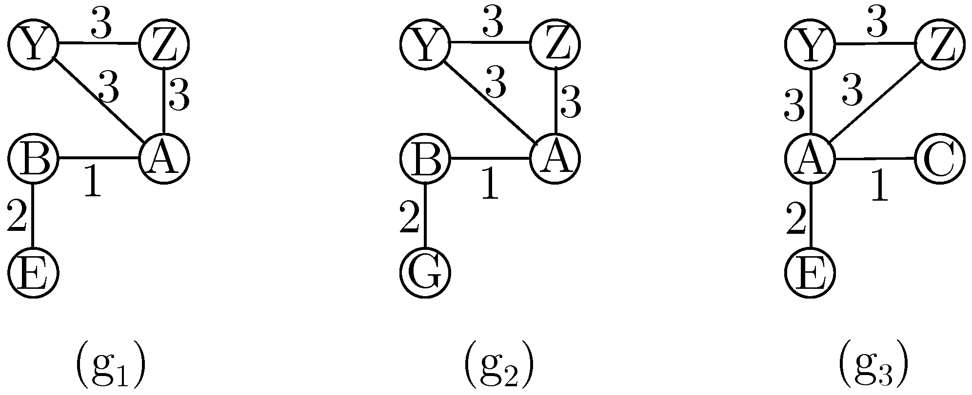
To demonstrate how the proposed algorithm mines frequent approximate subgraphs with structural and label variations, we applied AGCM-SLV to the small graph collection shown in Figure 4, varying the dissimilarity threshold ($\beta$) and introducing different label similarities in the node dictionary ($\gamma$) and edge dictionary ($\delta$).

In a first experiment, we set the support threshold ($\alpha$) to 100% and the dissimilarity threshold ($\beta$) to zero, resulting in AGCM-SLV mining one frequent subgraph, $\overline{)\mathrm{B}}$, as shown in

Table 2. Frequent subgraphs mined by AGCM-SLV in the graph collection of Figure 4 with $\alpha$ = 100% and $\beta$ = 0.

Frequent Subgraph	Occurrences
$\overline{)\mathrm{B}}$	$\overline{)\mathrm{B}}$ $g_1$, $\overline{)\mathrm{B}}$ $g_2$, $\overline{)\mathrm{B}}$ $g_3$

. Since no modifications are allowed, this frequent subgraph has an exact match.

In a second experiment, we set the support threshold ($\alpha$) to 100% and the dissimilarity threshold ($\beta$) to one, resulting in AGCM-SLV mining the additional frequent approximate subgraph $\overline{)\mathrm{B}}\frac{\mathrm{D}}{}\overline{)\mathrm{A}}$, having two frequent subgraphs in total, as shown in the first column of

Table 3. Frequent approximate subgraphs mined by AGCM-SLV with $\alpha$ = 100% and $\beta$ = 1.

Frequent Subgraph	Occurrences
$\overline{)\mathrm{B}}$	$\overline{)\mathrm{B}}$ $g_1$, $\overline{)\mathrm{B}}$ $g_2$, $\overline{)\mathrm{B}}$ $g_3$
$\overline{)\mathrm{B}}\frac{\mathrm{D}}{}\overline{)\mathrm{A}}$	$\overline{)\mathrm{B}}\frac{\mathrm{D}}{}\overline{)\mathrm{A}}$ $g_1$, $\overline{)\mathrm{B}}\frac{\mathrm{D}}{}\overline{)\mathrm{Z}}$ $g_2$, $\overline{)\mathrm{B}}\frac{\mathrm{E}}{}\overline{)\mathrm{A}}$ $g_3$, $\overline{)\mathrm{B}}\frac{\mathrm{F}}{}\overline{)\mathrm{A}}$ $g_3$

. These frequent approximate subgraphs do not present structural variations, as only a single modification in the occurrences is allowed. This modification can be a label substitution on a node or edge.

To demonstrate the label substitution, consider the frequent approximate subgraph $\overline{)\mathrm{B}}\frac{\mathrm{D}}{}\overline{)\mathrm{A}}$, which appears on $g_2$, the occurrence $\overline{)\mathrm{B}}\frac{\mathrm{D}}{}\overline{)\mathrm{Z}}$, where we have a node label substitution: the node label ‘A’ is substituted by the node label ‘Z’. Additionally, the frequent approximate subgraph $\overline{)\mathrm{B}}\frac{\mathrm{D}}{}\overline{)\mathrm{A}}$ has two occurrences with edge label substitutions on $g_3$: $\overline{)\mathrm{B}}\frac{\mathrm{E}}{}\overline{)\mathrm{A}}$ and $\overline{)\mathrm{B}}\frac{\mathrm{F}}{}\overline{)\mathrm{A}}$.

In a third experiment, we set the support threshold ($\alpha$) to 100% and increased the dissimilarity threshold ($\beta$) to two to allow for structural variations. With these parameter values, AGCM-SLV mines five additional frequent approximate subgraphs, having a total of seven mined frequent subgraphs, as shown in the first column of

Table 4. Frequent approximate subgraphs mined by AGCM-SLV with $\alpha$ = 100% and $\beta$ = 2.

Frequent Subgraph	Occurrences
$\overline{)\mathrm{B}}$	$\overline{)\mathrm{B}}$ $g_1$, $\overline{)\mathrm{B}}$ $g_2$, $\overline{)\mathrm{B}}$ $g_3$
$\overline{)\mathrm{B}}\frac{\mathrm{D}}{}\overline{)\mathrm{A}}$	$\overline{)\mathrm{B}}\frac{\mathrm{D}}{}\overline{)\mathrm{A}}$ $g_1$, $\overline{)\mathrm{B}}$ $g_2$, $\overline{)\mathrm{B}}\frac{\mathrm{B}}{}\overline{)\mathrm{Y}}$ $g_2$, $\overline{)\mathrm{B}}\frac{\mathrm{D}}{}\overline{)\mathrm{Z}}$ $g_2$, $\overline{)\mathrm{B}}$ $g_3$, $\overline{)\mathrm{B}}\frac{\mathrm{E}}{}\overline{)\mathrm{A}}$ $g_3$, $\overline{)\mathrm{B}}\frac{\mathrm{F}}{}\overline{)\mathrm{A}}$ $g_3$
$\overline{)\mathrm{B}}\frac{\mathrm{E}}{}\overline{)\mathrm{A}}$	$\overline{)\mathrm{B}}\frac{\mathrm{E}}{}\overline{)\mathrm{A}}$ $g_3$, $\overline{)\mathrm{B}}$ $g_1$, $\overline{)\mathrm{B}}\frac{\mathrm{A}}{}\overline{)\mathrm{A}}$ $g_1$, $\overline{)\mathrm{B}}\frac{\mathrm{D}}{}\overline{)\mathrm{A}}$ $g_1$, $\overline{)\mathrm{B}}$ $g_2$, $\overline{)\mathrm{B}}\frac{\mathrm{B}}{}\overline{)\mathrm{Y}}$ $g_2$, $\overline{)\mathrm{B}}\frac{\mathrm{D}}{}\overline{)\mathrm{Z}}$ $g_2$
$\overline{)\mathrm{B}}\frac{\mathrm{B}}{}\overline{)\mathrm{Y}}$	$\overline{)\mathrm{B}}\frac{\mathrm{B}}{}\overline{)\mathrm{Y}}$ $g_2$, $\overline{)\mathrm{B}}$ $g_1$, $\overline{)\mathrm{B}}\frac{\mathrm{A}}{}\overline{)\mathrm{A}}$ $g_1$, $\overline{)\mathrm{B}}\frac{\mathrm{D}}{}\overline{)\mathrm{A}}$ $g_1$, $\overline{)\mathrm{B}}$ $g_3$, $\overline{)\mathrm{B}}\frac{\mathrm{B}}{}\overline{)\mathrm{Y}}$ $g_2$, $\overline{)\mathrm{B}}\frac{\mathrm{D}}{}\overline{)\mathrm{Z}}$ $g_2$
$\overline{)\mathrm{B}}\frac{\mathrm{A}}{}\overline{)\mathrm{A}}$	$\overline{)\mathrm{B}}\frac{\mathrm{A}}{}\overline{)\mathrm{A}}$ $g_1$, $\overline{)\mathrm{B}}$ $g_2$, $\overline{)\mathrm{B}}\frac{\mathrm{B}}{}\overline{)\mathrm{Y}}$ $g_2$, $\overline{)\mathrm{B}}\frac{\mathrm{D}}{}\overline{)\mathrm{Z}}$ $g_2$, $\overline{)\mathrm{B}}$ $g_3$, $\overline{)\mathrm{B}}\frac{\mathrm{E}}{}\overline{)\mathrm{A}}$ $g_3$, $\overline{)\mathrm{B}}\frac{\mathrm{F}}{}\overline{)\mathrm{A}}$ $g_3$
$\overline{)\mathrm{B}}\frac{\mathrm{F}}{}\overline{)\mathrm{A}}$	$\overline{)\mathrm{B}}\frac{\mathrm{F}}{}\overline{)\mathrm{A}}$ $g_3$, $\overline{)\mathrm{B}}$ $g_1$, $\overline{)\mathrm{B}}\frac{\mathrm{A}}{}\overline{)\mathrm{A}}$ $g_1$, $\overline{)\mathrm{B}}\frac{\mathrm{D}}{}\overline{)\mathrm{A}}$ $g_1$, $\overline{)\mathrm{B}}$ $g_3$, $\overline{)\mathrm{B}}\frac{\mathrm{B}}{}\overline{)\mathrm{Y}}$ $g_2$, $\overline{)\mathrm{B}}\frac{\mathrm{D}}{}\overline{)\mathrm{Z}}$ $g_2$
$\overline{)\mathrm{B}}\frac{\mathrm{D}}{}\overline{)\mathrm{Z}}$	$\overline{)\mathrm{B}}\frac{\mathrm{D}}{}\overline{)\mathrm{Z}}$ $g_2$, $\overline{)\mathrm{B}}$ $g_1$, $\overline{)\mathrm{B}}\frac{\mathrm{A}}{}\overline{)\mathrm{A}}$ $g_1$, $\overline{)\mathrm{B}}\frac{\mathrm{D}}{}\overline{)\mathrm{A}}$ $g_1$, $\overline{)\mathrm{B}}$ $g_3$, $\overline{)\mathrm{B}}\frac{\mathrm{E}}{}\overline{)\mathrm{A}}$ $g_3$, $\overline{)\mathrm{B}}\frac{\mathrm{F}}{}\overline{)\mathrm{A}}$ $g_3$

.

To demonstrate the structural variations, consider the frequent approximate subgraph $\overline{)\mathrm{B}}\frac{\mathrm{D}}{}\overline{)\mathrm{A}}$ and its occurrence $\overline{)\mathrm{B}}$ on $g_2$, which requires two structural variations are required: the deletion of node $\overline{)\mathrm{A}}$ and its corresponding edge.

In a fourth experiment, we set the support threshold ($\alpha$) to 100% and the dissimilarity threshold ($\beta$) to two while providing label similarities in nodes through the node dictionary($\gamma$). This indicates that the node label ‘Z’ has 50% similarity with node label ‘A’ and node label ‘Y’ has 50% similarity with node label ‘A’. In this scenario, AGCM-SLV mines the seven frequent approximate subgraphs shown in the first column of Table 4, plus one frequent approximate subgraph shown in the first column of

Table 5. Additional frequent approximate subgraph mined by AGCM-SLV with $\alpha$ = 100%, $\beta$ = 2 and $\gamma$ with node label Z with 50% similarity to node label A and node label Y with 50% similarity to node label A.

Frequent Subgraph	Occurrences
$\overline{)\mathrm{A}}\frac{\mathrm{A}}{}\overline{)\mathrm{B}}\frac{\mathrm{D}}{}\overline{)\mathrm{A}}$	$\overline{)\mathrm{A}}\frac{\mathrm{A}}{}\overline{)\mathrm{B}}\frac{\mathrm{D}}{}\overline{)\mathrm{A}}$ $g_1$, $\overline{)\mathrm{Z}}\frac{\mathrm{D}}{}\overline{)\mathrm{B}}\frac{\mathrm{B}}{}\overline{)\mathrm{Y}}$ $g_2$, $\overline{)\mathrm{A}}\frac{\mathrm{E}}{}\overline{)\mathrm{B}}\frac{\mathrm{F}}{}\overline{)\mathrm{A}}$ $g_3$

.

To demonstrate the use of the node dictionary ($\gamma$), consider the occurrence $\overline{)\mathrm{Z}}\frac{\mathrm{D}}{}\overline{)\mathrm{B}}\frac{\mathrm{B}}{}\overline{)\mathrm{Y}}$ on $g_2$ of the frequent subgraph $\overline{)\mathrm{A}}\frac{\mathrm{A}}{}\overline{)\mathrm{B}}\frac{\mathrm{D}}{}\overline{)\mathrm{A}}$. In this scenario, the frequent node $\overline{)\mathrm{B}}$ was expanded to $\overline{)\mathrm{A}}$ through the labeled edge ‘D’, while the occurrence was expanded from $\overline{)\mathrm{B}}$ to $\overline{)\mathrm{Z}}$ through the labeled edge ‘D’. The substitution between the node labels ‘A’ and ‘Z’ requires a dissimilarity cost of 0.5. The frequent subgraph was then expanded from the frequent node $\overline{)\mathrm{B}}$ to $\overline{)\mathrm{A}}$ through the labeled edge ‘A’, and the occurrence was expanded from $\overline{)\mathrm{B}}$ to $\overline{)\mathrm{Y}}$ through the labeled edge ‘B’. The edge label ‘B’ is substituted with a dissimilarity cost of 1 between labels ‘B’ and ‘A’, as well as a substitution with a dissimilarity cost of 0.5 between the node labels ‘A’ and ‘Z’. As a result, the frequent subgraph $\overline{)\mathrm{A}}\frac{\mathrm{A}}{}\overline{)\mathrm{B}}\frac{\mathrm{D}}{}\overline{)\mathrm{A}}$ and its occurrence $\overline{)\mathrm{Z}}\frac{\mathrm{D}}{}\overline{)\mathrm{B}}\frac{\mathrm{B}}{}\overline{)\mathrm{Y}}$ on $g_2$ have a dissimilarity of 2.

In a fifth experiment, we set the support threshold ($\alpha$) to 100% and the dissimilarity threshold ($\beta$) to two, but by changing the label similarities in nodes through the node dictionary($\gamma$) file, which indicates that the node label ‘Z’ has 100% similarity with node label ‘A’ and node label ‘Y’ has 100% similarity with node label ‘A’. In this scenario, AGCM-SLV mines the three additional frequent subgraphs, as shown in the first column of

Table 6. Additional frequent approximate subgraphs mined by AGCM-SLV with $\alpha$ = 100%, $\beta$ = 2, and $\gamma$ indicates that node label ‘Z’ has a 100% similarity to node label ‘A’ and node label ‘Y’ has a 100% similarity to node label ‘A’.

Frequent Subgraph	Occurrences
$\overline{)\mathrm{A}}\frac{\mathrm{E}}{}\overline{)\mathrm{B}}\frac{\mathrm{F}}{}\overline{)\mathrm{A}}$	$\overline{)\mathrm{A}}\frac{\mathrm{E}}{}\overline{)\mathrm{B}}\frac{\mathrm{F}}{}\overline{)\mathrm{A}}$ $g_3$, $\overline{)\mathrm{A}}\frac{\mathrm{A}}{}\overline{)\mathrm{B}}\frac{\mathrm{D}}{}\overline{)\mathrm{A}}$ $g_1$, $\overline{)\mathrm{Y}}\frac{\mathrm{B}}{}\overline{)\mathrm{B}}\frac{\mathrm{D}}{}\overline{)\mathrm{Z}}$ $g_2$
$\overline{)\mathrm{B}}\frac{\mathrm{A}}{}\overline{)\mathrm{A}}\frac{\mathrm{C}}{}\overline{)\mathrm{A}}$	$\overline{)\mathrm{B}}\frac{\mathrm{A}}{}\overline{)\mathrm{A}}\frac{\mathrm{C}}{}\overline{)\mathrm{A}}$ $g_1$, $\overline{)\mathrm{B}}\frac{\mathrm{B}}{}\overline{)\mathrm{Y}}\frac{\mathrm{C}}{}\overline{)\mathrm{Z}}$ $g_2$, $\overline{)\mathrm{B}}\frac{\mathrm{D}}{}\overline{)\mathrm{Z}}\frac{\mathrm{C}}{}\overline{)\mathrm{Y}}$ $g_2$, $\overline{)\mathrm{B}}\frac{\mathrm{E}}{}\overline{)\mathrm{A}}\frac{\mathrm{G}}{}\overline{)\mathrm{Z}}$ $g_3$
$\overline{)\mathrm{B}}\frac{\mathrm{D}}{}\overline{)\mathrm{A}}\frac{\mathrm{C}}{}\overline{)\mathrm{A}}$

, for a total of 11 mined frequent subgraphs.

These additional frequent approximate subgraphs were mined due to increased similarity among certain node labels, allowing them to appear in all the graphs within the collection while fulfilling the support threshold. The occurrence $\overline{)\mathrm{Y}}\frac{\mathrm{B}}{}\overline{)\mathrm{B}}\frac{\mathrm{D}}{}\overline{)\mathrm{Z}}$ on $g_2$ of the frequent approximate subgraph $\overline{)\mathrm{A}}\frac{\mathrm{E}}{}\overline{)\mathrm{B}}\frac{\mathrm{F}}{}\overline{)\mathrm{A}}$ serves as an example. According to the node dictionary ($\gamma$), the node labels ‘Z’ and ‘Y’ are equivalent to ‘A’. The variations in the occurrence involve two modifications: the substitution of both edge labels.

Finally, in a sixth experiment, we set the support threshold ($\alpha$) to 100% and the dissimilarity threshold ($\beta$) to two. We introduced label similarities in edges through the edge dictionary($\beta$) and maintained the same label similarities in nodes. As before, according to the node dictionary($\gamma$), node labels ‘Z’ and ‘Y’ are considered 100% similar to node label ‘A’. Moreover, according to the edge dictionary ($\delta$), the edge label ‘F’ is 100% similar to the edge label ‘D’. In this scenario, AGCM-SLV mines an additional frequent approximate subgraph, as shown in the first column of

Table 7. Additional frequent subgraph mined by AGCM-SLV with $\alpha$ = 100%, $\beta$ = 2, $\gamma$ indicates that node label ‘Z’ has a 100% similarity to node label ‘A’ and node label ‘Y’ has a 100% similarity to node label ‘A’; and additionally, $\delta$ indicates that edge label ‘F’ has a 100% similarity to edge label ‘D’.

Frequent Subgraph	Occurrences

, resulting in a total of 12 mined frequent approximate subgraphs.

The additional frequent approximate subgraph was mined due to the introduction of the edge label dictionary ($\delta$) considering that edge label ‘F’ is equivalent to edge label ‘D’, finding the occurrence $\overline{)\mathrm{A}}\frac{\mathrm{E}}{}\overline{)\mathrm{B}}\frac{\mathrm{F}}{}\overline{)\mathrm{A}}$ on $g_3$. The variations in the occurrence involve two modifications: substituting the edge label ‘E’ with ‘A’ and deleting the edge labeled ‘C’.

5.2. Comparison Between AGCM-SLV and REAFUM

This section presents a comparison between our proposed algorithm (AGCM-SLV) and REAFUM, which is the most similar algorithm to ours reported in the literature. Section 5.2.1 analyzes the differences between the frequent subgraphs mined by both algorithms, while Section 5.2.2 compares the number of frequent subgraphs mined and the runtime spent by each algorithm.

5.2.1. Comparison of the Frequent Approximate Subgraphs Mined by Both Algorithms

A comparison of the frequent approximate subgraphs mined by AGCM-SLV and REAFUM was performed. Both algorithms present inherent similarities, such as mining frequent subgraphs in a dataset considering structural and label variations in nodes and edges; nevertheless, this comparison aims to focus on the key differences, such as that REAFUM is designed to mine only some frequent subgraphs, by selecting some representative graphs and performing a representative frequent approximate subgraph refinement. In contrast, AGCM-SLV aims to mine all frequent approximate subgraphs in the dataset. Moreover, REAFUM cannot assign partial similarities to labels in nodes and edges. Meanwhile, AGCM-SLV allows the definition of partial similarities among labels of nodes and edges. To ensure a fair analysis, some considerations were taken into account: only the approximate frequent subgraph mining stage of REAFUM was considered without selecting representative graphs and representative approximate frequent subgraph refinement. For AGCM-SLV, no partial similarities between labels were used, as REAFUM cannot use them.

In this experiment, the small graph collection depicted in Figure 5 was used to illustrate the differences between the frequent approximate subgraphs mined by both algorithms. The parameters set in both algorithms were a support threshold ($\alpha$) of $100\%$ and a dissimilarity threshold ($\beta$) of two, resulting in AGCM-SLV mining 31 frequent subgraphs, while REAFUM mined 20 frequent subgraphs. The results also indicated both algorithms mined 19 frequent approximate subgraphs in common; AGCM-SLV mined 12 additional frequent approximate subgraphs that REAFUM did not mine, while REAFUM mined one additional frequent approximate subgraph that AGCM-SLV did not mine.

The additional frequent approximate subgraph mined by REAFUM, as shown in Figure 6, is $\overline{)\mathrm{A}}\frac{1}{}\overline{)\mathrm{B}}\frac{2}{}\overline{)\mathrm{E}}$ on graph $g_1$, with occurrences $\overline{)\mathrm{A}}\frac{1}{}\overline{)\mathrm{B}}\frac{2}{}\overline{)\mathrm{G}}$ on graph $g_2$, and $\overline{)\mathrm{C}}\frac{1}{}\overline{)\mathrm{A}}\frac{2}{}\overline{)\mathrm{E}}$ on graph $g_3$. Unlike REAFUM, our algorithm analyzed $\overline{)\mathrm{A}}\frac{1}{}\overline{)\mathrm{B}}\frac{2}{}\overline{)\mathrm{E}}$ as a candidate subgraph and pruned it because its occurrence on graph $g_3$ exceeded the dissimilarity threshold, i.e., it did not meet the required support threshold. The occurrence on $g_3$ would require three modifications: The deletion of the edge from $\overline{)\mathrm{A}}$ to $\overline{)\mathrm{E}}$, the insertion of an edge from $\overline{)\mathrm{C}}$ to $\overline{)\mathrm{E}}$, and the substitution of the node label ‘C’ by the node label ‘B’, which exceeds the dissimilarity threshold of two.

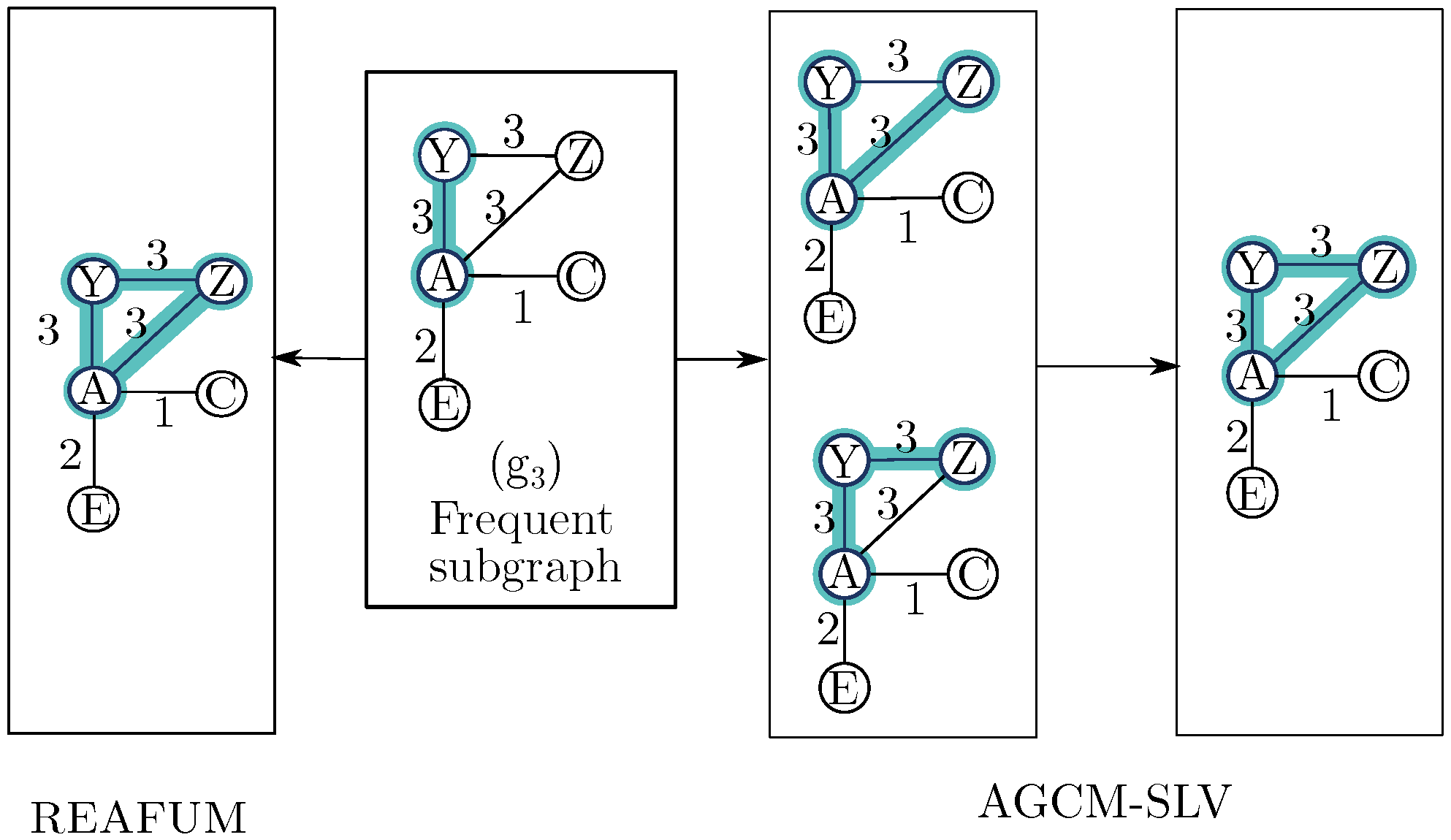
AGCM-SLV mined 12 frequent approximate subgraphs that REAFUM did not. To understand why this happens, the frequent subgraph expansion processes of both algorithms were analyzed. Both algorithms analyze the frequent subgraph’s neighboring nodes while building candidate subgraphs from a previously found frequent subgraph. However, REAFUM connects a neighboring node with all edges that connect it. In contrast, AGCM-SLV creates a separate candidate subgraph for each edge that connects a neighboring node, resulting in a greater diversity of frequent subgraphs. Figure 7 provides an example of this. This figure describes the frequent subgraph expansion process of $\overline{)\mathrm{Y}}\frac{3}{}\overline{)\mathrm{A}}$ in graph $g_3$. In AGCM-SLV, the node $\overline{)\mathrm{Z}}$ is expanded, creating three candidate frequent subgraphs: first, using the edge $\overline{)\mathrm{Y}}\frac{3}{}\overline{)\mathrm{Z}}$, then the edge $\overline{)\mathrm{A}}\frac{3}{}\overline{)\mathrm{Z}}$, and as a later expansion, both edges. In contrast, REAFUM expands node $\overline{)\mathrm{Z}}$ using both edges, resulting in just one candidate subgraph.

5.2.2. Comparison Regarding the Number of Frequent Approximate Subgraphs Mined and Runtime

In this experiment, we compared the performance of REAFUM and our proposed algorithm (AGCM-SLV) with a real-world dataset (PTC-FM [64]). We evaluated how the variation in the parameters $\alpha$ and $\beta$ impacts the number of frequent subgraphs mined and the runtime.

PTC-FM is a dataset that contains compounds labeled according to carcinogenicity in female mice. This dataset includes 349 graphs where nodes represent atoms labeled by atom type, and edges represent chemical bonds and are labeled by bond type.

This experiment uses specific portions of the PTC-FM dataset based on its size.

Table 8. Datasets built from PTC-FM for our experiment.

Dataset	Total Graphs	Average Nodes	Average Edges
1–10	10	16.8	17.1
11–20	10	14.2	14.7
21–30	10	11.9	12.6
31–40	10	12.2	13
1–20	20	15.5	15.9
21–40	20	12.05	12.8
41–60	20	13.1	13.45
61–80	20	14.2	14.3
1–30	30	14.3	14.8
31–60	30	12.8	13.3
61–90	30	13.2	13.3
91–120	30	13.93	14.37
1–40	40	13.77	14.35
41–80	40	13.65	13.88
81–120	40	13.25	13.6
121–160	40	14.12	14.3
1–50	50	13.12	13.56
51–100	50	13.34	13.66
101–150	50	14.58	14.9
151–200	50	15.46	16.02

shows the datasets built from PTC-FM for our experiment.

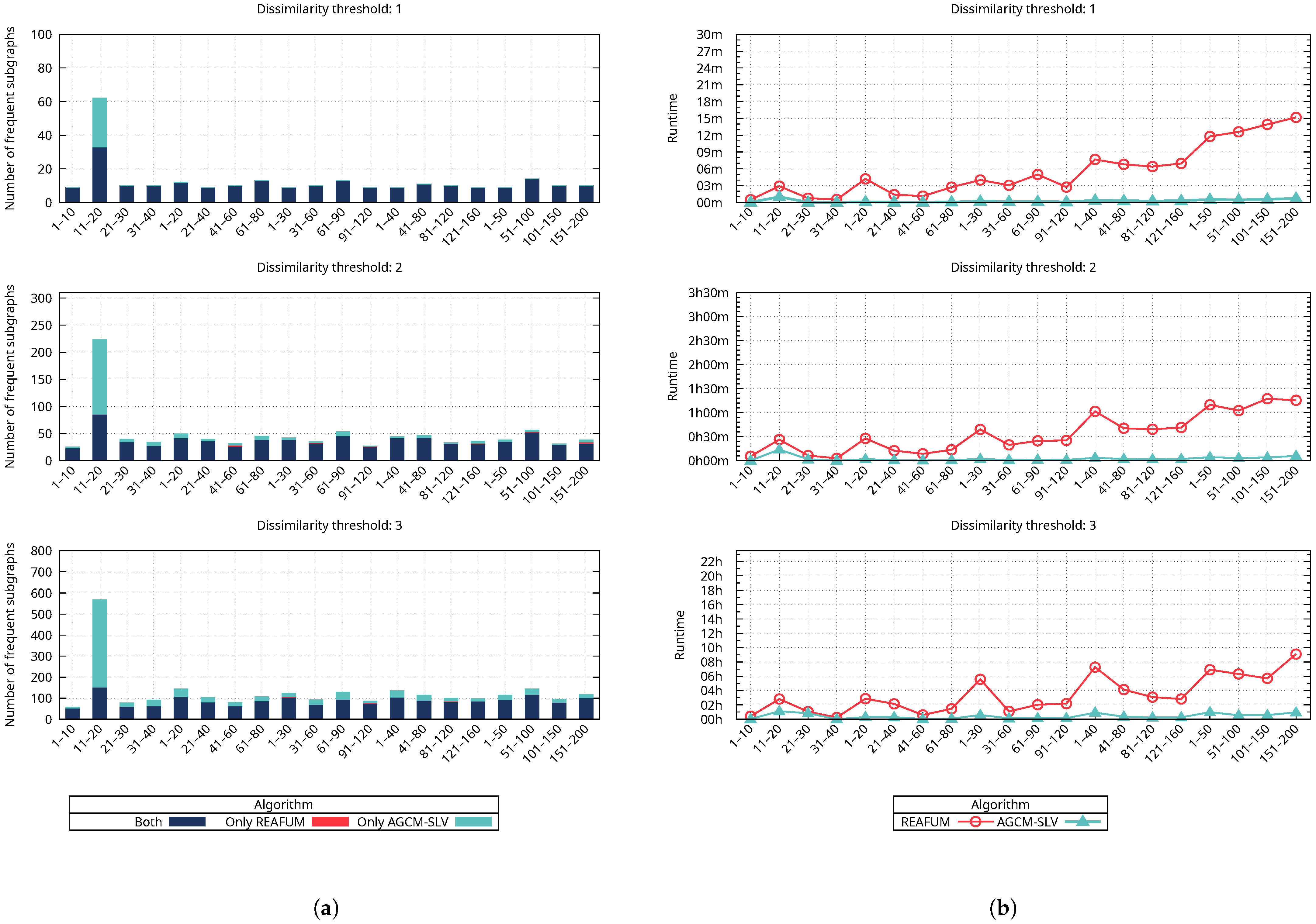
Figure 8a shows how the number of frequent approximate subgraphs mined is affected by varying the dissimilarity threshold, with the support threshold set constant at 90%. The figure contains three horizontal plots showing the number of frequent approximate subgraphs mined, each plot corresponding to a specific value of the dissimilarity threshold (1, 2, and 3). The colored bars represent the number of frequent approximate subgraphs mined for the different cases (both, only REAFUM, and only AGCM-SLV). It is important to emphasize that each plot has a different number of frequent subgraphs on the y-axis scale. In the first plot, when the dissimilarity threshold is 1, the number of frequent approximate subgraphs is up to 100; in the second plot, when the dissimilarity threshold is 2, the number of frequent approximate subgraphs is up to 310; and in the third plot, when the dissimilarity threshold is 3, the number of frequent approximate subgraphs extends up to 800. We need to focus on each plot to compare the number of frequent approximate subgraphs mined by both algorithms. The results reveal that while both algorithms mine most of the frequent subgraphs represented by a blue-colored bar, there are also cases where an algorithm mines additional frequent subgraphs represented by a cyan-colored bar for our proposed algorithm and a red-colored bar for REAFUM. Notice that the red-colored bars representing REAFUM in Figure 8a are not easily seen (see, for example, the second graph of Figure 8a in the last column corresponding to 121–150), since there are a few cases where a small number of frequent approximate subgraphs are mined only by REAFUM. To observe how varying the dissimilarity threshold impacts the number of frequent subgraphs mined, we compare the increase in frequent subgraphs mined across the three plots. The results show that both algorithms mine more frequent approximate subgraphs as the dissimilarity threshold increases.

Figure 8b shows the corresponding runtime in which the frequent approximate subgraphs of Figure 8a were mined by both algorithms. This figure also contains three horizontal plots, which, in this case, show the runtime of mining the frequent approximate subgraphs for both algorithms. Each plot corresponds to a dissimilarity threshold value (1, 2, and 3); the number of frequent approximate subgraphs mined is represented by colored bars for the different cases (both, only REAFUM, and only AGCM-SLV), and the runtime is represented by different line colors for each algorithm (REAFUM and AGCM-SLV). It is important to emphasize that each plot has a different time scale on the y-axis. In the first plot, when the dissimilarity threshold is 1, the runtime is less than 30 min; in the second plot, when the dissimilarity threshold is 2, the runtime is less than 3 h and 30 min; and in the third plot, when the dissimilarity threshold is 3, the runtime grows to more than 22 h. To compare the runtime of both algorithms, we need to focus on each plot, where it is observed that our algorithm’s runtime is shorter in all cases. To observe how varying the dissimilarity threshold impacts the runtime, we compare the increase in the runtime across the three plots. The results show that as the dissimilarity threshold increases, the runtime increases for both algorithms, which is related to the increase in the number of frequent approximate subgraphs mined. However, the runtime increases significantly for REAFUM compared to our proposed algorithm.

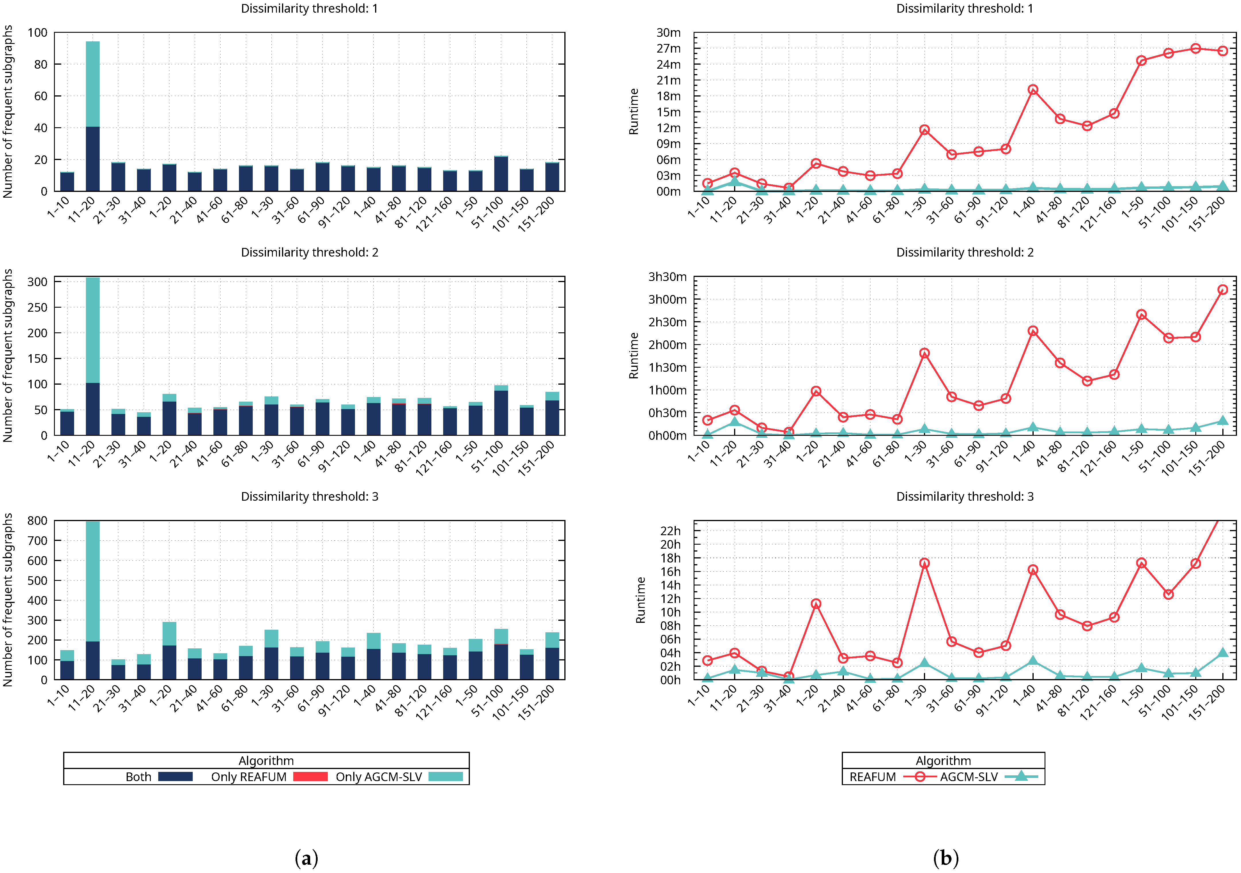
Figure 9 is similar to Figure 8, except that it uses a constant support threshold of 80%. Figure 9a contains three horizontal plots showing the number of frequent approximate subgraphs mined, one for each dissimilarity threshold value (1, 2, and 3). The colored bars represent the number of frequent approximate subgraphs mined for the different cases (both, only REAFUM, and only AGCM-SLV). It is important to analyze how the support threshold impacts the number of frequent approximate subgraphs that are mined. At an 80% support threshold, more frequent subgraphs are mined compared to a 90% support threshold, as fewer occurrences are required for a subgraph to be considered frequent, as shown across the plots.

Figure 9b, on the other hand, contains three horizontal plots, one for each dissimilarity threshold value (1, 2, and 3), showing the corresponding runtime for both algorithms. The red line represents REAFUM, and the blue line represents AGCM-SLV. The results reveal an increase in the number of frequent approximate subgraphs mined as a result of a smaller support threshold, which also impacts the rise in runtime. As with the previous experiment, if the dissimilarity threshold increases, there is a consistent growth in the number of frequent subgraphs and runtime. However, the results show that our proposed algorithm’s runtime increases at a slower rate than REAFUM’s, which is consistent with the previous experiment.

These experiments reveal that varying the dissimilarity or support thresholds impacts the number of frequent approximate subgraphs mined and the runtime for REAFUM and the proposed algorithm. However, our proposed algorithm mines more frequent subgraphs in a shorter runtime than REAFUM’s.

5.3. Analysis of the Performance of AGCM-SLV

We evaluated the performance of our proposed algorithm, AGCM-SLV, on the real-world PTC dataset [64] by analyzing how variations in the dissimilarity threshold ($\beta$) and support threshold ($\alpha$) impact both the number of frequent approximate subgraphs mined and the runtime.

The PTC dataset [64] contains compounds labeled according to carcinogenicity in male mice (MM), male rats (MR), female mice (FM), and female rats (FR). In these four graph collections, the nodes represent atoms and are labeled by atom type, and the edges represent chemical bonds and are labeled by bond type.

Table 9. Description of PTC datasets.

Dataset	Total Graphs	Average Nodes	Average Edges
PTC-FM	349	14.11	14.48
PTC-FR	351	14.56	15.00
PTC-MM	336	13.97	14.32
PTC-MR	344	14.29	14.69

shows the number of graphs in each graph collection and the average number of nodes and edges for the four PTC graph collections.

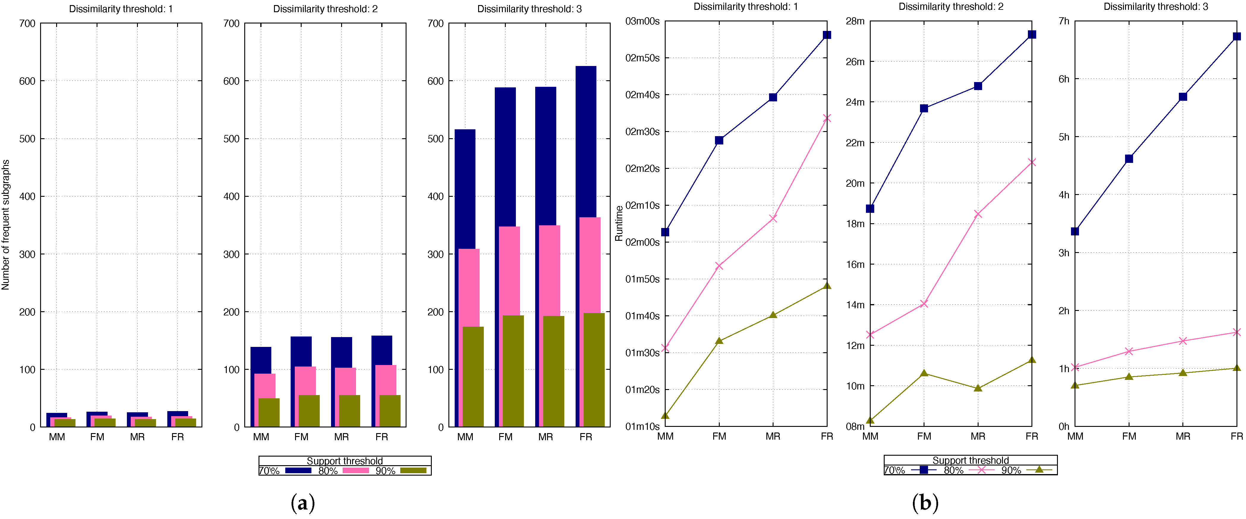
Figure 10a shows the impact of varying the dissimilarity and support thresholds on the number of frequent approximate subgraphs mined. This figure contains three vertical plots showing the number of frequent approximate subgraphs mined across the four graph collections of PTC (FM, FR, MM, and MR). Each plot corresponds to a specific dissimilarity threshold value (1, 2, or 3). In each plot, the colored bars represent the number of frequent approximate subgraphs mined for each support threshold (70%, 80%, and 90%).

To observe the impact of varying the dissimilarity threshold, we compare the increase in the number of frequent approximate subgraphs across the three plots. The results show that as the dissimilarity threshold increases, the number of frequent approximate subgraphs mined also increases. This is because allowing more modifications increases the number of occurrences per candidate subgraph that fulfills the dissimilarity threshold, leading to more frequent approximate subgraphs being mined.

On the other hand, to observe the impact of varying the support threshold, we compare the variation within each plot with the different colored bars. The results reveal that the number of frequent approximate subgraphs mined increases as the support threshold decreases. This is because it is more likely for a frequent approximate subgraph to appear in fewer graphs within the graph collection.

Figure 10b shows the corresponding runtime for mining the frequent approximate subgraphs shown in Figure 10a. This figure also contains three vertical plots, which indicate the runtime of mining the frequent approximate subgraphs across the four graph collections of PTC (FM, FR, MM, and MR). Each plot corresponds to a specific dissimilarity threshold value (1, 2, or 3). The colored lines represent the runtimes for each support threshold (70%, 80%, and 90%).

To observe the impact of varying the dissimilarity threshold on runtime, we need to compare the increase in the runtime across the three plots. It is important to emphasize that each plot has a different timescale on the y-axis. In the first plot, the runtime is less than 3 min with a dissimilarity threshold of 1; in the second plot, it is less than 28 min with a dissimilarity threshold of 2; and in the third plot, it extends up to 7 h with a dissimilarity threshold of 3. As the dissimilarity threshold increases, the runtime also increases because of the rise in the number of frequent approximate subgraphs mined.

On the other hand, to observe how varying the support threshold impacts the runtime, we must compare the variation within each plot with the color lines representing the support thresholds. The runtime increases as the support threshold decreases due to the increase in the number of frequent approximate subgraphs mined. The results reveal that the runtime increases at a higher rate when the dissimilarity threshold is increased compared with the support threshold. For example, when the dissimilarity threshold is 1, the runtime for all the different support thresholds is a few minutes, and it increases to several hours when the dissimilarity threshold is 3.

5.4. Scalability

The PTC dataset was used for the proposed algorithm’s scalability tests. PTC is a dataset composed of four graph collections: PTC-FM, PTC-FR, PTC-MM, and PTC-MR. These collections are described in Table 9. The four PTC collections were combined into a single collection containing 1380 graphs with an average of 14.24 nodes and 14.63 edges per graph.

Multiple tests were conducted using portions of the collections described above based on their size. Each test was performed using dissimilarity thresholds of 1 and 2. Regarding the support threshold, a constant support threshold was set to 70% because a higher threshold did not produce any frequent subgraphs. In each test, runtime and maximum RAM usage were measured to evaluate the resources required to execute our algorithm.

Initially, we ran our algorithm on 100 graphs from both collections, using the parameters described above. Subsequent tests were performed by adding 100 graphs per experiment until all the graphs in the collection were included.

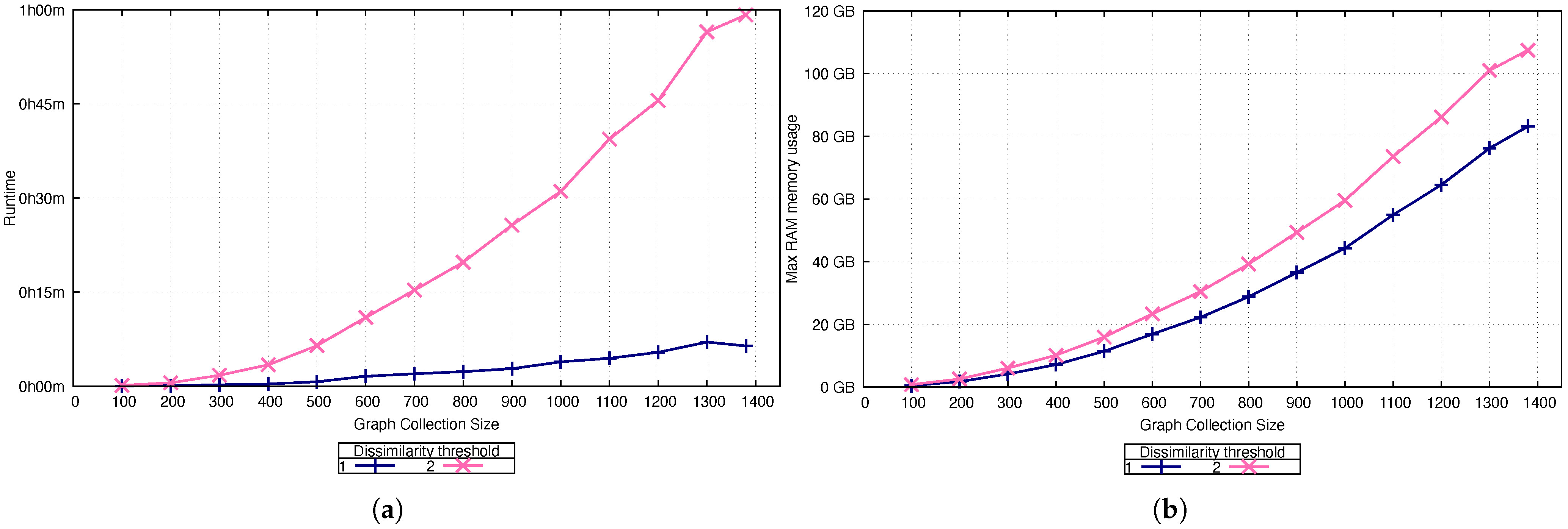
The measured runtimes are presented in Figure 11a, and the maximum memory usage is shown in Figure 11b. We evaluated all 1380 graphs in the collection with both dissimilarities in less than 1 h using a maximum of 120 GB of RAM.

These tests exhibit growth in terms of runtime and memory usage; however, the runtime increased at a faster rate than the memory usage. The results reveal that increasing the dissimilarity threshold significantly affected the runtime, leading to longer runtimes. However, this effect does not extend to the memory usage.

5.5. Impact of Random White Noise in the Proposed Algorithm

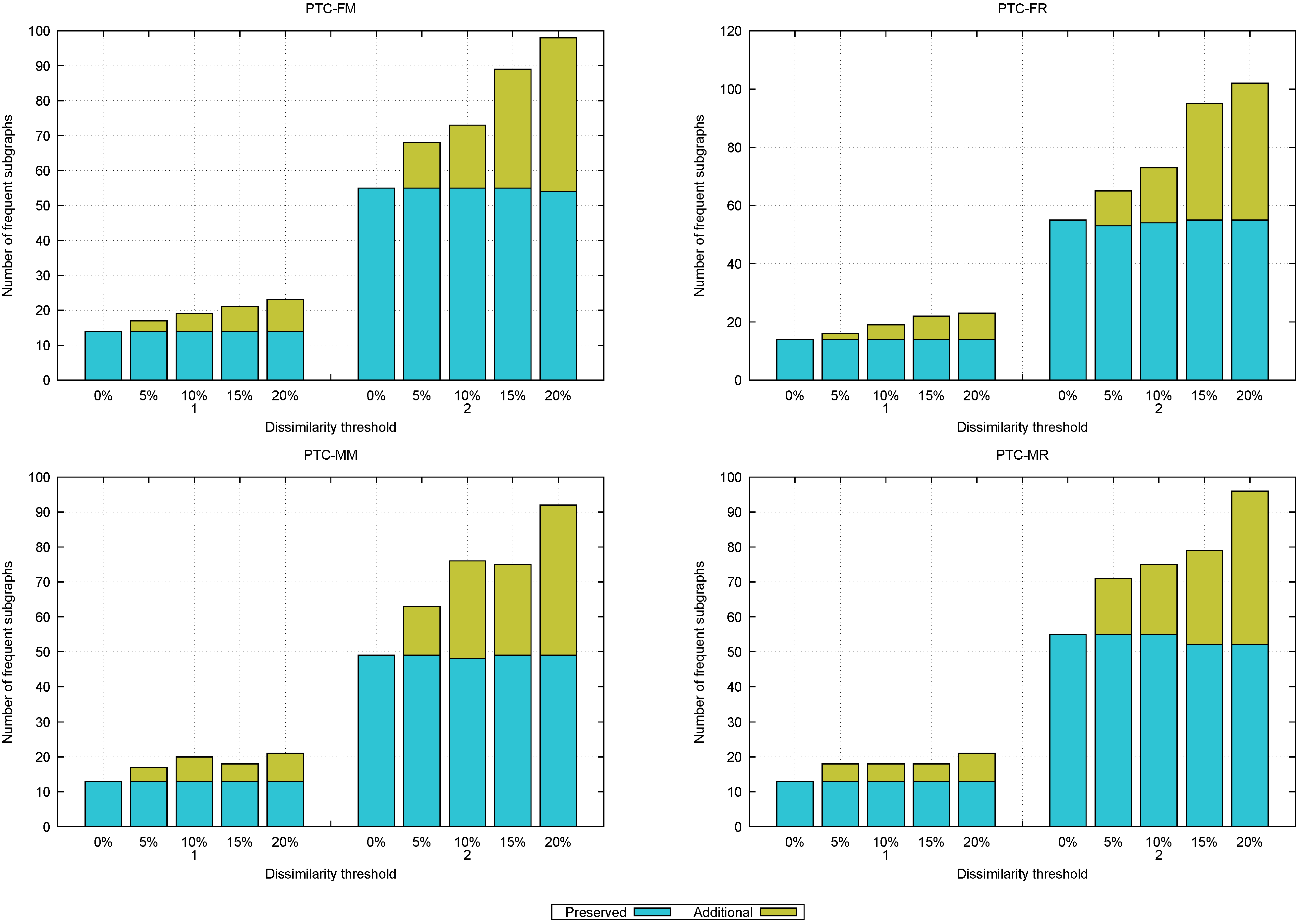
This experiment evaluates the impact of random white noise on the proposed algorithm for mining frequent approximate subgraphs with structural and label variations. To perform this experiment, we introduced 5%, 10%, 15%, and 20% of noise to the PTC datasets in Table 9. Then, we apply our proposed algorithm to the noisy datasets to mine frequent approximate subgraphs at the different noise levels.

Noise was added randomly, including the addition of nodes with their corresponding edges, the addition of only edges, and label substitutions in both nodes and edges. For each noisy dataset, we mined frequent approximate subgraphs using AGCM-SLV, employing dissimilarity thresholds of 1 and 2. In all cases, we used a support threshold of 90%. The frequent approximate subgraphs mined from the original, noise-free datasets served as reference.

Figure 12 shows the impact of different levels of noise on the frequent approximate subgraphs mined. This figure contains four bar graphs, each corresponding to a different PTC dataset (FM, FR, MM, and MR). In each graph, the x-axis represents different noise levels (0% (noise-free), 5%, 10%, 15%, and 20%) grouped by dissimilarity thresholds (1 and 2). The bars are stacked vertically, with each bar’s height indicating the number of frequent approximate subgraphs mined. Each bar is split into two segments: a blue segment labeled Preserved that represents the frequent approximate subgraphs preserved from those mined in the original noise-free (0% noise level) dataset, and a green segment labeled Additional that represents the new frequent approximate subgraphs mined at the current noise level.

The results reveal that as noise increases, the number of frequent approximate subgraphs also increases, suggesting that certain subgraphs become frequent because the noise introduces additional occurrences. These occurrences allow previously infrequent subgraphs to now satisfy the required support threshold and become frequent. Moreover, when noise is included, the majority (99.49% on average) of the frequent approximate subgraphs mined from the noise-free dataset (see 0% in Figure 12) were preserved, indicating the algorithm’s tolerance to white noise.

Table 10. Percentage of frequent approximate subgraphs preserved across different noise levels, compared to those mined in the noise-free datasets, employing a support threshold $\alpha =90\%$ and dissimilarity thresholds $\beta =1$ and $\beta =2$.

Noise Level	$\mathit{\beta }=1$	$\mathit{\beta }=2$
PTC- FM
5%	100%	100%
10%	100%	100%
15%	100%	100%
20%	100%	98.18%
PTC- FR
5%	100%	96.36%
10%	100%	98.18%
15%	100%	100%
20%	100%	100%
PTC- MM
5%	100%	100%
10%	100%	97.96%
15%	100%	100%
20%	100%	100%
PTC- MR
5%	100%	100%
10%	100%	100%
15%	100%	94.55%
20%	100%	94.55%

shows that every frequent subgraph (100%) is maintained when the dissimilarity threshold is 1, and 98.88% are preserved when the dissimilarity threshold is 2. Thus, only a few of the frequent approximate subgraphs are lost. This happens because occurrences disappear (i.e., an occurrence that previously required only two modifications may now need more, making it no longer match the frequent approximate subgraph). As a result, these subgraphs no longer satisfy the required support threshold.

Due to the random nature of the introduced noise, datasets with higher noise levels may sometimes maintain more frequent approximate subgraphs than those with lower noise levels. As the noise level increases, additional frequent approximate subgraphs may appear that are not present in the noise-free dataset. However, the majority of frequent subgraphs from the original dataset are consistently maintained across the different noise levels, which shows the algorithm’s low sensitivity to white noise.

6. Conclusions

Mining frequent approximate subgraphs with structural and label variations in an undirected graph collection has been scarcely studied in the literature. In this paper, we have proposed AGCM-SLV, an algorithm for mining frequent approximate subgraphs with structural and label variations in graph collections. Our algorithm follows a depth-first traversal strategy starting from frequent nodes (which are single-node subgraphs) and expands them, verifying both the support and dissimilarity thresholds while discarding those that do not meet the defined thresholds.

To assess the proposed algorithm, we conducted experiments comparing it with REAFUM, the most similar algorithm to ours reported in the literature. From these experiments, we can conclude that, due to AGCM-SLV expanding frequent subgraphs through their neighboring edges instead of only their neighboring nodes (as REAFUM does), our proposed algorithm mines frequent subgraphs that REAFUM cannot mine in a shorter runtime.

On the other hand, we also performed experiments to analyze the runtime behavior of AGCM-SVL, varying dissimilarity and support thresholds, on real-world datasets. These experiments reveal that AGCM-SLV’s runtime increases at a higher rate when the dissimilarity threshold is increased compared with the support threshold.

Our scalability experiments allow us to conclude that although AGCM-SLV exhibits fast growth in terms of runtime and memory usage as the collection grows. The increase in runtime is faster than the increase in memory usage, especially when increasing the dissimilarity threshold.

Finally, we assessed the impact of random white noise in the graph collection when our proposed algorithm is applied for mining frequent approximate subgraphs with structural and label variations. This experiment allows us to conclude that AGCM-SLV is tolerant to white noise, since more than 99% of the frequent approximate subgraphs mined without noise are preserved in noise conditions.

In our experiments, we address approximate label similarities through dictionaries, as this approach enables the easy definition of similarities among labels across different domains. However, the algorithm can be easily adapted to include user-defined similarity functions for more complex or domain-specific scenarios.

The main limitation of the proposed algorithm is its time complexity, as the algorithm can only be used on relatively small collections of graphs. However, to our knowledge, it is the first algorithm to address the mining of all frequent approximate subgraphs with structural and label variations in graph collections allowing user-defined partial similarities between node and edge labels. This limitation presents an area of opportunity for the development of more efficient algorithms that can operate with larger collections of graphs. Another interesting problem to address as future work is the development of algorithms for mining frequent subgraphs with structural and label variations in dynamic collections of graphs or for streaming data problems, where the graphs change over time. Extending the proposed algorithm to handle more complex relationships between graph nodes, such as those involving multiple edges between them, as in multigraphs, is a task that also deserves future study. Finally, evaluating our algorithm in a real-life application to solve a real-life problem is a very important line of future research.