An Adapter and Segmentation Network-Based Approach for Automated Atmospheric Front Detection

Abstract

This study presents AD-MRCNN, an advanced deep learning framework for automated atmospheric front detection that addresses two critical limitations in existing methods. First, current approaches directly input raw meteorological data without optimizing feature compatibility, potentially hindering model performance. Second, they typically only provide frontal category information without identifying individual frontal systems. Our solution integrates two key innovations: 1. An intelligent adapter module that performs adaptive feature fusion, automatically weighting and combining multi-source meteorological inputs (including temperature, wind fields, and humidity data) to maximize their synergistic effects while minimizing feature conflicts; the utilized network achieves an average improvement of over 4% across various metrics. 2. An enhanced instance segmentation network based on Mask R-CNN architecture that simultaneously achieves (1) precise frontal type classification (cold/warm/stationary/occluded), (2) accurate spatial localization, and (3) identification of distinct frontal systems. Comprehensive evaluation using ERA5 reanalysis data (2009–2018) demonstrates significant improvements, including an 85.1% F1-score, outperforming traditional methods (TFP: 63.1%) and deep learning approaches (Unet: 83.3%), and a 31% reduction in false alarms compared to semantic segmentation methods. The framework’s modular design allows for potential application to other meteorological feature detection tasks. Future work will focus on incorporating temporal dynamics for frontal evolution prediction.

1. Introduction

In atmospheric science, the significance of studying weather fronts lies in the frequent occurrence of severe weather changes near them. For example, regions near frontal systems are often accompanied by extreme weather phenomena such as heavy precipitation, storms, and hail, and fronts are frequently the center of thunderstorms [1,2,3]. Statistics show that frontal precipitation accounts for 51% of global extreme precipitation, and up to 90% of extreme precipitation events are associated with mid-latitude fronts [2]. Therefore, the identification and analysis of fronts are crucial tasks in weather analysis and forecasting, holding significant research importance for socio-economic and even military applications.

Currently, automated methods for front identification mainly fall into two categories: numerical front analysis (NFA) and machine learning (ML) methods. NFA primarily involves selecting a parameter input into a manually defined function and using a threshold to diagnose whether a front exists. Such methods include the gradient method (Gτ), thermal front parameter (TFP) [4,5,6], wind change (WC) [7], F-diagnosis [8], and the process of growing frontiersmen (PGF) [9], among others. However, these methods face limitations such as sensitivity to grid resolution, noise from second derivatives, and challenges in threshold determination [10,11]. The wind-shift method has rarely detected warm fronts [12]. Recent advancements in NFA, such as the dynamic state index (DSI) proposed by [13], attempt to address these issues by incorporating diabatic processes, but they still struggle with feature conflicts and systematic biases.

To overcome these limitations, machine learning-based approaches have gained prominence. Early efforts utilized convolutional neural networks (CNNs) for localized frontal classification [14,15], but these methods suffered from fragmented results due to subregion division. Fully convolutional networks (FCNs) improved upon CNNs by enabling end-to-end processing, yet they failed to capture multi-scale features [16]. The introduction of U-Net architectures marked a significant advancement by leveraging skip connections for deeper feature fusion [17], but challenges remained in resolving feature conflicts among meteorological inputs. Recent studies, such as [18], have explored hybrid models combining U-Net with attention mechanisms to enhance feature compatibility, while [11] proposed the UNET3+ model to improve multi-scale feature aggregation. Despite these efforts, existing methods still face two critical limitations:

• Input Feature Compatibility: direct input of raw meteorological data without adaptive feature fusion leads to suboptimal model performance due to feature conflicts.
• Output Granularity: semantic segmentation networks only provide frontal category information without distinguishing individual frontal systems [16,19].

To address these challenges, this study proposes AD-MRCNN, a novel framework that integrates two key innovations:

• Intelligent Adapter Module: This module performs adaptive feature fusion by dynamically weighting and combining multi-source meteorological inputs (e.g., temperature, wind fields, humidity). It resolves feature conflicts through a normalization–weighting–fusion pipeline, enhancing the synergy of input features while suppressing noise. The adapter’s design is inspired by recent work in feature fusion [17,20], which demonstrated the effectiveness of adaptive weighting in meteorological applications.
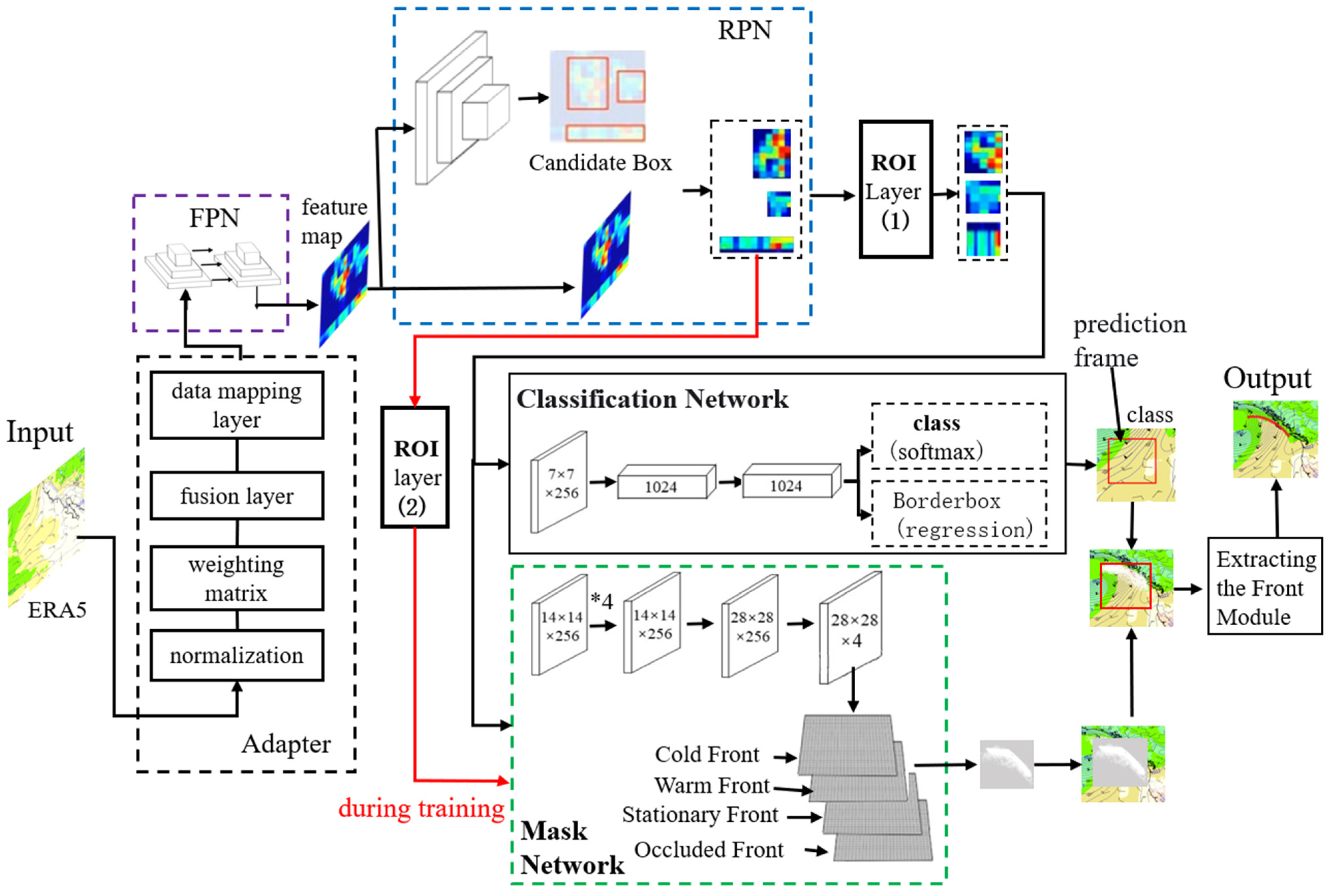
• Enhanced Instance Segmentation Network: Based on Mask R-CNN, this network extends traditional semantic segmentation by simultaneously classifying frontal types (cold/warm/stationary/occluded), localizing spatial boundaries, and identifying distinct frontal systems. The integration of feature pyramid networks (FPNs) and ROI Align ensures precise multi-scale feature extraction, as validated in [20,21].

Our approach is rigorously evaluated using ERA5 reanalysis data (2009–2018), demonstrating superior performance over existing methods (e.g., 85.1% F1-score vs. Unet’s 83.3%). The modular design of AD-MRCNN also allows for potential extensions to other meteorological tasks, such as trough line detection or frontal evolution prediction [22,23].

2. Data and Method

2.1. Data

The input data used in this study were obtained from the fifth-generation global atmospheric reanalysis dataset (ERA5) produced by the European Centre for Medium-Range Weather Forecasts (ECMWF). This dataset encompasses a wide range of global meteorological observations and model output data for the atmosphere, ocean, and land surface from 1979 to the present.

The selected variables include the following:

• Temperature (T), U-wind (U), V-wind (V), and specific humidity (q) at 850 hPa;
• Dew point temperature (T_d) at 2 m;
• Mean sea level pressure (P_msl).

The spatial coverage ranges from 37° W to 165° W and 10° N to 74° N, with a horizontal resolution of 0.25° × 0.25° and a temporal resolution of 3 h. The study period spans from 2009 to 2018, with the following data splits:

• Test set: 2009.
• Training set: 2010–2017.
• Validation set: 2018.

Table 1. Details of the input data used in this study.

Coverage	37° to 165° W
	10° to 74° N
Resolution ratio	0.25° × 0.25°
Interval time	3 h
Meteorological elements	2 m above ground	Dewpoint Temperature (Td2m)
	850 hPa	Temperature (T850hpa)
		specific humidity(q)
		U, Vwind
		Pressure ($P_{\mathrm{m}\mathrm{s}\mathrm{l}}$)
Data set classification	Training Set (2010–2017)
	Validation Set (2018)
	Test set (2009)

provides detailed information on the input data used in this study.

This study produces frontal data for air mass labeling using surface bulletins from the U.S. Weather Prediction Center (WPC). Each frontal system is represented by a series of discrete latitude–longitude coordinate pairs, which are temporally and spatially consistent with the selected ERA5 reanalysis data. To facilitate neural network training, the WPC frontal data undergoes the following processing steps: resolution enhancement, curve fitting, expansion, and labeling of frontal bounding boxes and categories.

Figure 1 illustrates the transformation of WPC frontal data into training labels for the network. Step A involves increasing the resolution of the original WPC frontal data and applying bilinear interpolation to fit the points into a smooth curve. Step B expands the frontal data by marking adjacent non-frontal grid points as frontal points and iterating this expansion three times, thereby increasing the number of frontal grid points to mitigate severe class imbalance. Step C involves using image annotation software (LabelImg, Install labelimg: Enter the following command in cmd, pip install labelimg-i pypi.tuna.tsinghua.edu.cn/simple) to label the bounding boxes and categories of the frontal systems.

2.2. Method

The AD-MRCNN network model proposed in this study is illustrated in Figure 2. It primarily consists of three components: an adapter module, an instance segmentation network, and a frontal line extraction module. The overall workflow of the AD-MRCNN model is as follows: First, six types of meteorological element data at a given time point are input into the adapter, where normalization, data value weighting via weight adjustment, convolutional feature fusion, and mapping to a 0–255 range are performed. Next, the processed data are fed into a pre-trained feature extraction backbone network (FPN) to obtain abstract feature maps. These feature maps are then input into a region proposal network (RPN) to generate a series of candidate ROI bounding boxes. The corresponding regions of these candidate boxes in the feature maps are cropped and sent to the ROI Align layer, where feature maps of varying sizes are resized into uniformly dimensioned abstract feature maps. Finally, these maps are separately input into three branches: one for predicting frontal category grid points, one for bounding box regression, and the mask branch for extracting frontal segmentation information within the identified regions.

2.2.1. Adapter for Adaptive Fusion of Multiple Meteorological Elements

To facilitate the training of the network and improve its accuracy, the proposed model in this study incorporates an adapter, which primarily consists of four components: a normalization layer, a weight layer, a fusion layer, and a data mapping layer. The normalization layer is employed to eliminate the dimensional differences among multi-meteorological-element data, thereby enhancing the model’s convergence speed and precision. This study adopts the Z-score normalization method, with the calculation formula as follows:

$$Z={\displaystyle \frac{X-\mu }{\sigma }},$$

(1)

Here, Z is the normalized value, X is the original meteorological element data, μ is the mean of the original meteorological element data, and σ is the standard deviation of the original meteorological element data.

The weight layer in the adapter can adjust the importance scale among different elements, thereby effectively resolving feature conflicts caused by special weather conditions and geographical locations among multiple meteorological elements. It assigns a weight value to each meteorological element at every grid point within the identification area. During network training, these weight values are continuously adjusted using labels to filter out conflicts and modulate the strength of the correlation between multi-meteorological element features and frontal systems.

Considering that multiple meteorological elements collectively form a systematic representation relative to frontal systems, the fusion layer in the adapter is employed to extract the composite features of these elements. This facilitates the subsequent network in extracting highly abstract features, thereby improving training efficiency and recognition accuracy. The input data shape is [256, 512, 6], where 256 and 512 represent the dimensions of the 2D array in the identification area (the size and dimensions are determined based on practical application requirements; the data shape selected in this paper is chosen merely for computational convenience). The third dimension, 6, indicates that the fusion layer has six input channels, corresponding to six weight matrices. The output data shape of the fusion layer is [256, 512, 3].

Since instance segmentation networks primarily process image data, the 3-channel fused feature data are mapped to the range [0, 255] before being input into the instance segmentation network to ensure better compatibility.

$$Y=a+{\displaystyle \frac{b-a}{X_{max}-X_{min}}}.\left(X-X_{min}\right),$$

(2)

Among them, a and b are the minimum and maximum values of the input data mapping interval, respectively. In this paper, a is set to 0 and b is set to 255. $X_{max}$ is the maximum value in the dataset X, and $X_{min}$ is the minimum value in the dataset X. Y represents the mapped data.

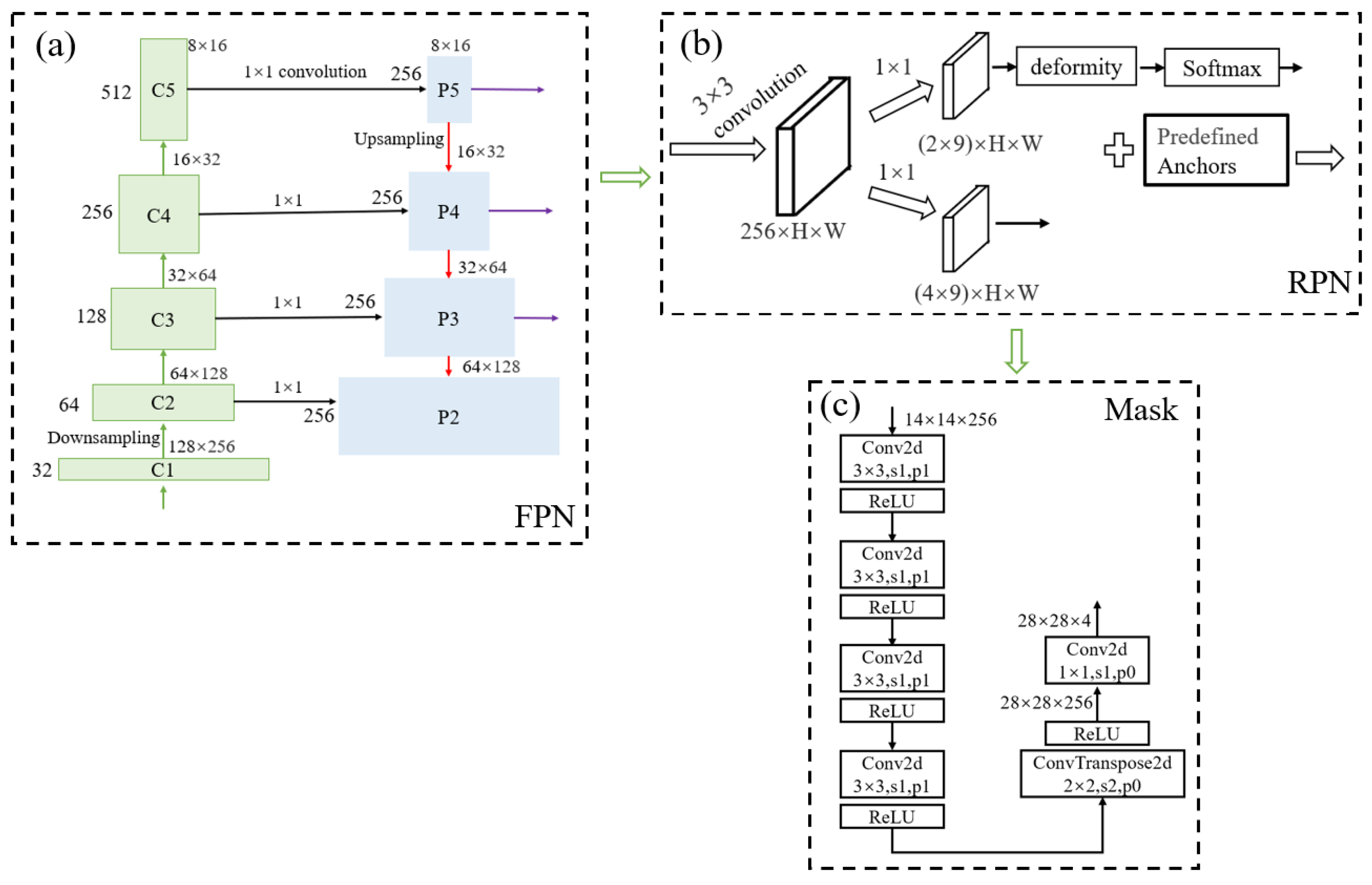
2.2.2. FPN Network Module for Extracting Multi-Meteorological-Element Fusion Features

In the feature extraction module, to enhance the performance of small object detection, the model adopts the feature pyramid network (FPN) [24], a feature fusion mechanism that combines the multi-resolution scale prediction of the SSD network with the multi-resolution feature fusion architecture of Unet. Its operational mechanism is illustrated in Part A of Figure 3 and consists of three components: bottom-up convolution, top-down upsampling, and lateral feature fusion.

Each convolutional layer in the FPN module comprises three operations: convolution, max pooling, and ReLU activation. In all convolutional operations, the kernel size is 3, with a padding of 1 and a stride of 1. All pooling layers use a kernel size of 2, with a padding of 1 and a stride of 1.

2.2.3. The RPN (Region Proposal Network) Module for Obtaining Frontal Candidate Bounding Boxes

The RPN (region proposal network) is used to extract high-quality ROI (region of interest) bounding boxes for atmospheric frontal candidate regions, which are then utilized in subsequent stages. It consists of four main components:

• Anchor Generator—Generates initial anchor boxes based on feature scales and aspect ratios. The scales are set to 8, 16, and 32, while the aspect ratios are 0.5, 1, and 2, resulting in a total of 9 anchor boxes.
• Anchor Target Generator—Determines which anchor boxes are positive samples (fronts) and which are negative samples (non-fronts) by computing the IoU (Intersection over Union) between anchors and ground truth.
• RPN Loss—Computes the classification and regression losses during training.
• Proposal Generator—Produces refined candidate regions through post-processing steps, such as clipping out-of-bound boxes and removing excessively small boxes, to obtain high-confidence ROI proposals.

As illustrated in Figure 3b, the RPN operates via two parallel branches:

• The upper branch classifies anchors into positive/negative samples using a softmax function.
• The lower branch predicts bounding box regression offsets to adjust anchor positions for better localization.

This structure enables efficient and accurate extraction of frontal candidate regions for further analysis.

2.2.4. RoI Align Layer for Handling Frontal Candidate Regions

Within the ROI Align layer, feature maps of varying sizes are transformed into abstract feature maps with consistent dimensions, which are then used by subsequent classification and mask network modules to classify and regress each previously detected ROI, ultimately outputting the final classes and bounding boxes for front detection.

The candidate boxes output by the ROI Align layer may deviate from the ground truth bounding boxes (IoU < 0.5), necessitating fine-tuning to bring them closer to the true target boxes and achieve more accurate localization of the candidate boxes. To better describe the bounding box regression method, we use a four-dimensional vector (x, y, w, h) to represent the window, where (x, y) denotes the center point of the window, and (w) and (h) represent its width and height, respectively. G is denoted as the ground truth bounding box. The bounding box regression is achieved through a mapping function (f($P_x$, $P_y$, $P_w$, $P_h$) = (${\widehat{G}}_x$, ${\widehat{G}}_y$, ${\widehat{G}}_w$, ${\widehat{G}}_h$)), such that (${\widehat{G}}_x$, ${\widehat{G}}_y$, ${\widehat{G}}_w$, ${\widehat{G}}_h$) ≈ ($G_x$, $G_y$, $G_w$, $G_h$). Among them, ($G_x$, $G_y$, $G_w$, $G_h$) represent the true values, and (${\widehat{G}}_x$, ${\widehat{G}}_y$, ${\widehat{G}}_w$, ${\widehat{G}}_h$) represent the predicted values. Boundary box regression utilizes translation and scaling transformations to achieve mapping. The calculation formula for translation transformation is as follows:

$$\left\{\begin{array}{c}{\widehat{G}}_x=P_w{d}_x\left(P\right)+P_x\\ {\widehat{G}}_y=P_h{d}_y\left(P\right)+P_y\end{array}\right.$$

(3)

The calculation formula for scale transformation is as follows:

$$\left\{\begin{array}{c}{\widehat{G}}_w=P_{w}exp\left(d_w\right(P\left)\right)\\ {\widehat{G}}_h=P_{h}exp\left(d_w\right(P\left)\right)\end{array}\right.$$

(4)

Among them, $d_{*}\left(P\right)$ (* represents x, y, w, h) is a set of four linear functions based on [pooling] _5. Here, we denote the feature as ${\varnothing }_5$(P), so $d_{*}\left(P\right)=w_{*}^T{\varnothing }_5\left(P\right)$. The solution expression for $w_{*}$ is

$$w_{*}={arg}_{w_{*}}min\sum ^N{(t_{*}^i-{\widehat{w}}_{*}^T{\varnothing }_5(P^i)}^2+\lambda {‖{\widehat{w}}_{*}‖}^2$$

The translation amount ($t_x$, $t_t$) and scaling amount ($t_w$,$t_h$) are represented as follows:

$$t_x={\displaystyle \frac{G_x-P_x}{P_w}} ,$$

(5)

$$t_y={\displaystyle \frac{G_y-P_y}{P_h}} ,$$

(6)

$$t_w=log\left({\displaystyle \frac{G_w}{P_w}} \right),$$

(7)

$$t_h=log\left({\displaystyle \frac{G_h}{P_h}} \right),$$

(8)

2.2.5. The MASK Network Module for Obtaining Binary Masks

The mask branch network module is illustrated as part C in Figure 3. It adopts a fully convolutional network (FCN) architecture for semantic segmentation. Notably, the softmax function is deliberately omitted in this module to prevent the high-scoring categories from suppressing low-scoring ones. This design avoids the potentially detrimental coupling relationship where all categories compete against each other due to the constraint that their prediction probabilities must sum to 1. Instead of using softmax, the predicted category from the classification branch network is directly employed to extract the corresponding mask, thereby eliminating inter-category competition. Such a decoupling strategy helps improve detection accuracy. Each ROI mask contains four categories corresponding to cold fronts, warm fronts, stationary fronts, and occluded fronts in frontal analysis.

It should be noted that during model training, both category prediction and mask generation are performed simultaneously. During prediction, after obtaining the frontal category results for grid points, these results are then fed into the mask network to generate the corresponding binary masks.

2.3. The Training of the Network

2.3.1. The Loss of the Network

The loss of the model consists of four components: the cross-entropy loss (CELoss) [25] and DLoss [26] for the classification branch, the regression loss for bounding boxes, and the loss for the mask branch.

During training, the classification network module employs both the DLoss function and the CELoss function. The DLoss function measures the similarity between the network’s recognition results and the sample labels, with training focusing more on the mining of frontal regions. However, it may suffer from loss saturation issues. Therefore, using DLoss alone does not yield optimal results. To address this, CELoss—which calculates the average loss per grid point—is incorporated for combined use. The functions are expressed as follows:

$$DLoss=1-{\displaystyle \frac{2*\left|y\cap \stackrel{\wedge }{y}\right|+smooth}{{\left|y\right|}^2+{\left|\stackrel{\wedge }{y}\right|}^2+smooth}},$$

(9)

where y represents the network’s frontal identification result; ŷ denotes the sample label; |y∩ŷ| indicates the number of intersecting grid points between y and ŷ; |y| and |ŷ| represent the number of grid points in y and ŷ, respectively; and smooth is a smoothing parameter (set to 0.1 in this paper). The purpose of squaring the denominator term is to accelerate the convergence speed.

For the classification task and mask branch, the loss calculation employs the CELoss function, which is expressed by the following formula:

$$CELoss=-{\displaystyle \frac{1}{N}}{\displaystyle \sum _{n=1}^N{\displaystyle \sum _{C=1}^C{y}_c^{(n)}\log ({\stackrel{\wedge }{y}}_c^{(n)})}},$$

(10)

Here, N represents the number of samples, C represents the number of classes, y denotes the predicted results, and ŷ denotes the ground truth labels.

The loss function formula for the bounding box regression task is expressed as follows:

$$Loss=\sum _i^N{{(t}_{*}^i-{\widehat{w}}_{*}^T{\varnothing }_5\left(P^i\right))}^2+\lambda {‖{\widehat{w}}_{*}‖}^2,$$

(11)

Here, ∅₅(P) represents the eigenvector, $t_{*}$ is the translation amount, $w_{*}$ denotes the parameters to be learned (* indicates x, y, w, h), and $\lambda {‖{\widehat{w}}_{*}‖}^2$ is the L₂ regularization term.

2.3.2. The Parameter Settings Related to Training the Network

During model training, hyperparameter tuning is performed using the training and validation datasets. Due to the depth of the network, to ensure that the output of the ReLU activation function does not completely vanish, the Kaiming method (He initialization) [27] is first employed to initialize the network parameters. The network utilizes stochastic gradient descent with a mini-batch size of 8 [28] and a momentum of 0.7. To help the gradient descent method escape local minima or saddle points, thereby finding better local optima and improving the model’s robustness and generalization capability, a cyclical learning rate is adopted during training. The maximum value of the cyclical learning rate [29] is set to ${10}^{-2}$, the minimum to ${10}^{-5}$, with a step size of 5 and a shrinkage factor of 2. Each cycle involves the learning rate decreasing from the maximum to the minimum value and then returning to the maximum, after which the learning rate is divided by the shrinkage factor. The maximum number of training iterations is set to 100, but early stopping is triggered if there is no improvement in validation loss for 30 consecutive iterations.

2.4. Model Prediction

During model prediction, the mask network obtains the most accurate candidate bounding box and a single-channel 28 × 28 feature map from the first ROI Align layer. These are then resized to match the predicted target candidate box dimensions and overlaid onto the corresponding region of the original multi-meteorological-element visualization map to generate the mask. A threshold is subsequently applied to convert this mask into a binary image—specifically, areas with predicted values exceeding the threshold (set at 0.5 in this study) are classified as frontal zones, while the remaining regions are designated as background (non-frontal). This process yields the frontal category information, bounding box data, and mask output for the identified region at a specific time. Building on this, the model’s frontal line extraction module further refines the results by performing two operations within the mask area: first, selecting the maximum temperature gradient value per row, followed by a curve-fitting operation to ultimately derive the final frontal identification results.

3. Results and Discussion

3.1. Evaluation Metrics

From the perspectives of fairness and comprehensiveness, this paper adopts accuracy (ACC), precision (P), recall (R), mean intersection over union (mIoU), and the F₁ score—to assess the performance of various methods on the dataset in the experiments. For a detailed introduction to the types of indicators, refer to [30,31]. Their calculation equations are as follows:

$$ACC\left(Y,\widehat{Y}\right)={\displaystyle \frac{1}{n}}\sum _{i=1}^n\delta \left(y_i,{\widehat{y}}_i\right),$$

(12)

Here, Y represents the true labels, Ŷ denotes the identified frontal surfaces, n indicates the total number of frontal surfaces in all labels, and the Dirac delta δ(.) is an indicator function where δ(.) = 1 when $y_i={\widehat{y}}_i$, otherwise δ(.) = 0.

$$P={\displaystyle \frac{TP}{TP+FP}},$$

(13)

$$R={\displaystyle \frac{TP}{TP+FN}},$$

(14)

$$F_1=2{\displaystyle \frac{P\times R}{P+R}},$$

(15)

$${IoU}_i={\displaystyle \frac{{TP}_i}{{TP}_i+{FP}_i+{FN}_i}},$$

(16)

$$mIoU={\displaystyle \frac{1}{N}}\sum _{i=1}^N{IoU}_i,$$

(17)

Among them, i represents the frontal category, and N denotes the total number of frontal categories (including non-frontal classes), which is five in this study. TP represents the total number of accurately predicted fronts, while FP indicates the total number of fronts misidentified as non-fronts. FN denotes the total number of non-fronts misidentified as fronts.

The evaluation in this study targets frontal objects, considering an identification as correct when the distance between the labeled and recognized results is within nine grid points. This criterion accounts for errors arising from both the expansion of network labels during data preprocessing and the post-processing of network identification results.

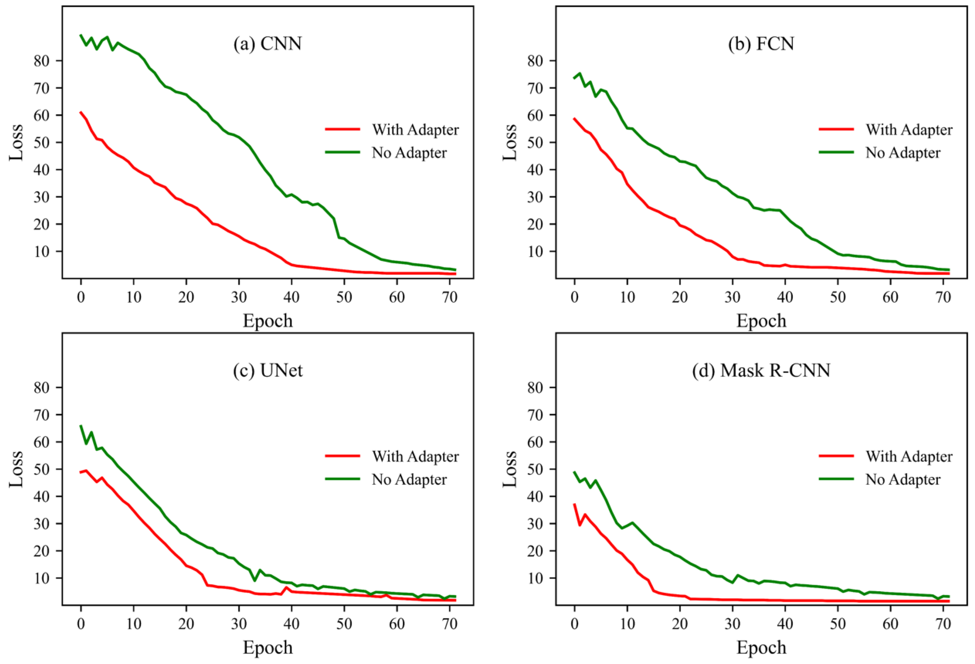
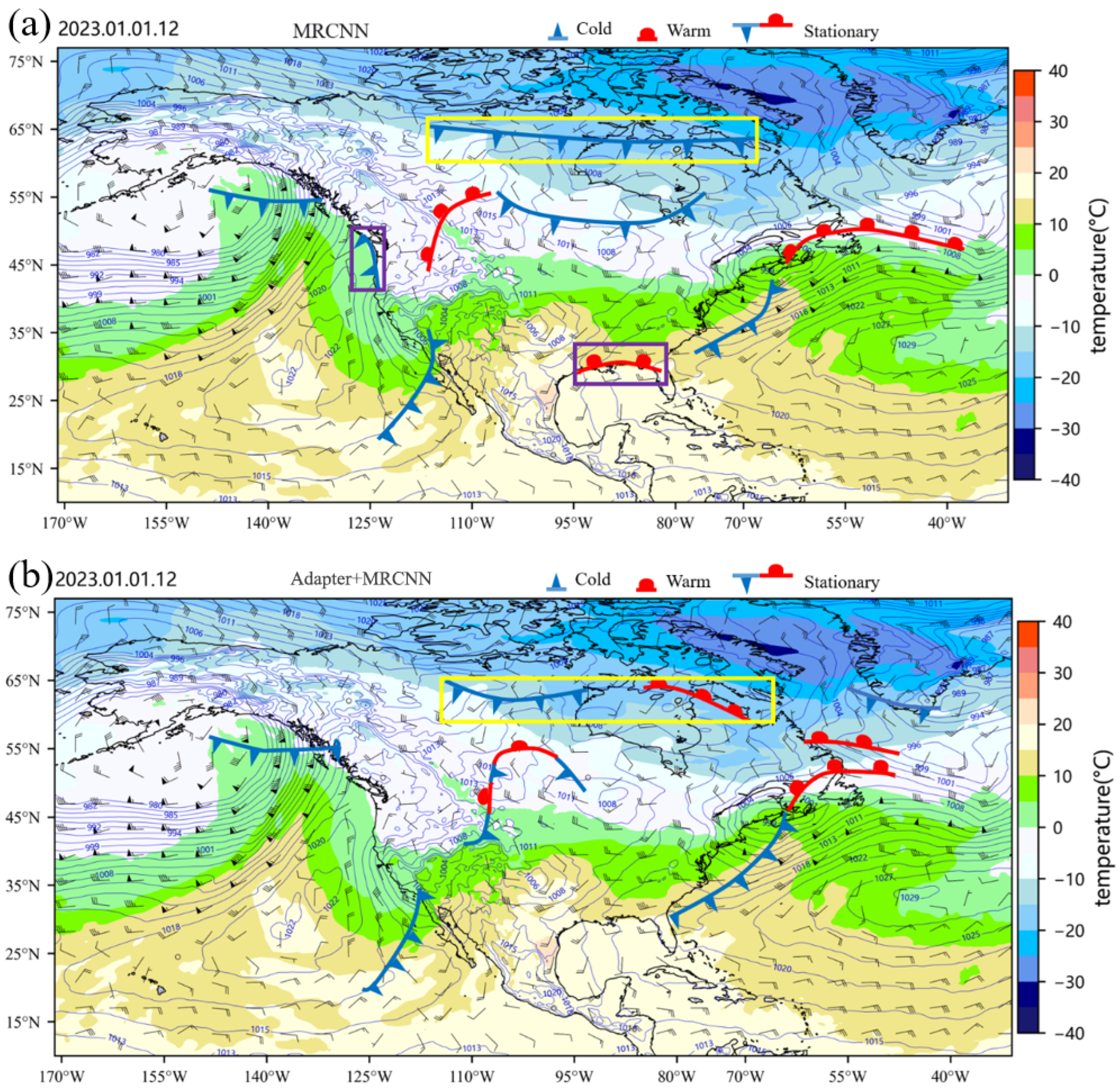
3.2. Experiment on the Effectiveness of Adapter

To verify whether incorporating adapter modules into current machine learning methods for automatic atmospheric front identification is conducive to network training and improves the accuracy of front identification, this section conducts experiments on the effectiveness of adapters. The experimental approach involves comparing four types of networks—CNN, FCN, Unet, and MRCNN—with and without adapter modules in terms of training loss, training epochs, and identification results across multiple evaluation metrics, namely ACC (accuracy), P (precision), R (recall), and F₁.

Figure 4 presents a comparison of training loss and epochs for the four types of networks with and without adapters under identical experimental settings. The figure reveals that for all four networks, the training loss decreases when using adapters, and the number of epochs required for the loss to stabilize is significantly reduced by an average of approximately 10 epochs. This indicates that adding adapters to current machine learning methods for front identification facilitates network training, thereby demonstrating the effectiveness of employing adapters in the proposed model of this study.

Under identical experimental setups, the final evaluation results of the eight networks (including the four baseline networks and their adapter-augmented variants) on the test set are presented in

Table 2. The scores of the adapter effectiveness experiment across multiple evaluation metrics.

Network Category	ACC	R	F1	mIoU
CNN	73.0%	65.0%	66.4%	47%
Adapter + CNN	76.7%	70.2%	69.7%	52.3%
FCN	75.1%	74.5%	74.9%	56%
Adapter + FCN	78.5%	79.7%	82.0%	60.1%
UNet	77.3%	83.3%	83.3%	63%
Adapter + UNet	80.9%	85.9%	85.8%	68%
MRCNN	79.2%	84.1%	81.6%	72%
AD-MRCNN	83.5%	86.8%	85.1%	77%

. The table demonstrates that all evaluation metrics for the four baseline networks improved by over 3% after incorporating the adapter modules, indicating that adding adapters to current machine learning networks for automatic front identification is effective. The improvement in network performance by the adapter is consistent with the studies in References [17,20]. This improvement can be attributed to two main reasons:

• The application of adapter modules in deep learning and their optimization effects on network training have been extensively studied. The literature [21,22] demonstrates the role of adapters in resolving feature conflicts and facilitating feature fusion. The weight layers within the adapter module filter out feature conflicts among multiple meteorological elements while suppressing strong non-frontal features and enhancing weak frontal features. This enables the network to efficiently and accurately learn the multi-element characteristics of fronts. Such feature conflicts primarily arise under specific weather conditions or geographical locations, where certain meteorological elements may exhibit abnormally strong non-frontal features (while others remain normally weak) or exceptionally weak frontal features (while others appear strongly frontal).
• The fusion layer in the adapter integrates features from multiple meteorological elements. By leveraging the systematic nature of fronts, it helps the network better approximate the complex patterns between frontal systems and multi-element composite features. This not only facilitates network training but also enhances the accuracy of front identification.

Additionally, we conducted a visualization of the ablation experiment results with and without the adapter on the MRCNN network, as shown in Figure 5. Figure 5a displays the visualization of frontal identification by the MRCNN network, while Figure 5b shows incorporating the adapter. A comparison reveals that Figure 5a identifies an additional frontal region within the purple box compared to Figure 5b; however, this region does not actually exist. This discrepancy arises because the MRCNN network performs poorly in distinguishing strong non-frontal meteorological features. For instance, the constant temperature zone at the land–sea boundary within the purple box is mistakenly identified as a frontal feature due to its strong meteorological characteristics. In contrast, with the adapter, the corresponding region in Figure 5b is correctly recognized as a non-frontal area. Furthermore, the yellow box in Figure 5a marks a cold front, whereas the corresponding region in Figure 5b contains both a cold front and a warm front. This occurs because the MRCNN network without the adapter fails to effectively resolve conflicts between meteorological features and frontal properties caused by special weather conditions or geographical factors, leading to the extraction of erroneous features. In contrast, the network with the adapter can accurately determine whether multi-meteorological features under such conditions represent frontal characteristics.

Special weather conditions include scenarios such as differing radiation conditions, evaporation–condensation dynamics, vertical motion variations, or the movement of cold air masses and cold fronts from land to sea. These conditions often weaken the temperature gradient across the frontal zone, making thermal features less pronounced. The adapter’s weighting layer enhances these weak frontal features by assigning higher weights. Special geographical locations, such as constant temperature zones near coastlines, can exhibit strong temperature differences due to varying underlying surface properties, often accompanied by wind disparities. Similarly, areas where plateaus meet plains may show temperature discrepancies due to differing station elevations. For such non-frontal regions with strong thermal signals, the adapter’s weighting layer assigns low weights to their meteorological features, enabling correct identification as non-frontal zones.

Moreover, the adapter’s fusion layer integrates multi-meteorological features, facilitating the network’s accurate learning of composite characteristics for different frontal types. This is evident in the yellow boxes of Figure 5a,b, where (a) only identifies a cold front, and (b) correctly distinguishes both a cold front and a warm front.

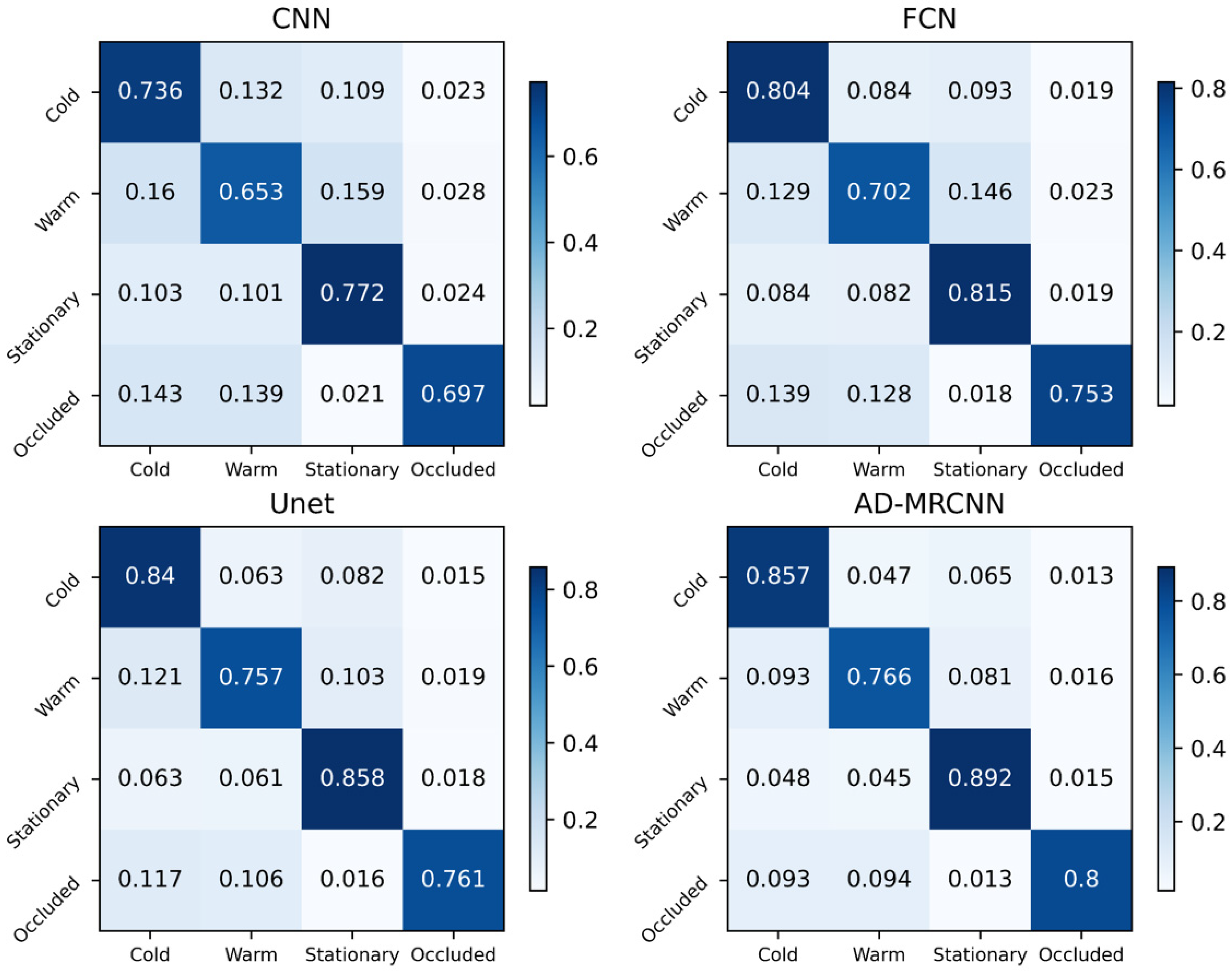
3.3. Multi-Method Comparative Experiment

This section compares the proposed AD-MRCNN model with six existing frontal identification methods on the same dataset and experimental setup, employing multiple evaluation metrics to validate the performance of AD-MRCNN in frontal identification. The final results are presented in

Table 3. Evaluation results of multiple atmospheric front identification methods.

Methods	ACC	P	R	${\mathit{F}}_1$	mIoU
$G_{\tau }$	65.6%	60.7%	57.3%	59.0%	×
TFP	69.6%	64.5%	61.8%	63.1%	×
F-diagnose	71.2%	65.2%	63.7%	64.5%	×
CNN [17]	73.0%	67.8%	65.0%	66.4%	47%
FCN	75.1%	76.9%	74.5%	74.9%	56%
U-Net [19]	77.3%	83.4%	83.3%	83.3%	63%
AD-MRCNN	83.5%	85.2%	86.8%	85.1%	77%

, from which the following conclusions can be drawn:

• Among traditional numerical frontal analysis methods, as the number of diagnostic factors increases from one to two and the diagnostic functions become more complex, the scores across all evaluation metrics show continuous improvement.
• Machine learning methods achieve significantly higher overall scores across multiple evaluation metrics compared to traditional numerical frontal analysis methods. This is because current machine learning approaches for automatic frontal identification take multiple meteorological elements as input, capturing the systematic and comprehensive characteristics of fronts by integrating diverse meteorological features. In contrast, traditional numerical methods rely on relatively singular meteorological elements, simpler functions, and face challenges in determining appropriate thresholds. The performance differences between traditional numerical methods and machine learning methods in meteorological front identification have been supported by research [23].
• Among machine learning methods, semantic segmentation-based approaches score lower than instance segmentation-based methods. This is primarily because instance segmentation networks, in addition to providing category and location information like semantic segmentation networks, also identify which specific frontal system each grid point belongs to, offering more detailed objective frontal information.

The superior performance of the AD-MRCNN model is consistent with the studies [24,32]. Next, in order to better evaluate the accuracy of each method in identifying frontal categories, we visualized the confusion matrices of four methods—CNN, FCN, Unet, and AD-MRCNN—on the test set for the identification of four frontal types (cold, warm, stationary, occluded), as shown in Figure 6. The analysis method of the confusion matrix is detailed in [33]. Since the total number of identified fronts in the test set is large, each row of the confusion matrix in Figure 6 is normalized by dividing the values by the total number of the corresponding frontal category and expressed as percentages, allowing for a more intuitive comparison of recognition performance across categories.

The results demonstrate that the accuracy of the four methods in identifying each frontal category gradually improves with increasing network complexity and refinement. Among them, AD-MRCNN achieves the highest accuracy in classifying all four frontal types, with the fewest misclassifications into other frontal categories. Additionally, the number of fronts misclassified as non-frontal cases consistently decreases across the four methods, with AD-MRCNN exhibiting the lowest such errors. This indicates that the AD-MRCNN model outperforms other methods in accurately identifying various frontal types, thereby achieving the highest overall frontal recognition accuracy.

4. Conclusions

This study presents AD-MRCNN, a novel deep learning framework for automated atmospheric front detection, addressing two critical limitations in existing methods: (1) suboptimal feature compatibility from raw meteorological inputs and (2) lack of instance-level frontal identification. Our key findings and contributions are summarized as follows:

1. Adapter Module Enhances Feature Fusion and Training Efficiency

The intelligent adapter module dynamically weights and fuses multi-source meteorological data (temperature, wind fields, humidity), resolving feature conflicts through a normalization–weighting–fusion pipeline. Ablation experiments demonstrated that adding the adapter reduced training epochs by ~10 (Figure 4), indicating faster convergence. Improved classification metrics by 3–5% across CNN, FCN, U-Net, and MRCNN (Table 2). Suppressed false alarms (Figure 5), particularly in regions with strong non-frontal signals (e.g., land–sea boundaries).

2. Instance Segmentation Outperforms Semantic Segmentation

Unlike traditional semantic segmentation (U-Net, FCN), AD-MRCNN provides instance-level identification, distinguishing individual frontal systems while classifying frontal types (cold/warm/stationary/occluded). Comparative experiments (Table 3) showed an 85.1% F1-score, surpassing U-Net (83.3%) and traditional methods (TFP: 63.1%), a 31% reduction in false alarms compared to semantic segmentation approaches, and a higher precision in frontal categorization (Figure 6), with fewer misclassifications (e.g., cold vs. warm fronts).

3. Robust Performance Across Meteorological Conditions

The adapter’s adaptive weighting mechanism improved detection in challenging scenarios, such as weak thermal gradients (e.g., cold air mass movement over oceans) and strong non-frontal signals (e.g., coastal temperature contrasts). The Mask R-CNN backbone with ROI Align ensured precise localization, even for small-scale fronts.

4. Future Directions

Future work includes generalizing AD-MRCNN to other meteorological tasks, such as trough line detection and cyclone tracking; integrating temporal dynamics by incorporating time-series data for frontal evolution prediction; and testing the model in real-time forecasting systems with higher-resolution inputs.

In summary, AD-MRCNN advances automated front detection by combining adaptive feature fusion with instance-aware segmentation, achieving higher accuracy, better spatial precision, and improved robustness compared to existing methods. The modular design ensures flexibility for broader applications in meteorological feature detection.

References

1. Garner, J. A study of synoptic-scale tornado regimes. E-J. Sev. Storms Meteorol. 2013, 8, 1–25. [Google Scholar] [CrossRef]
2. Catto, J.L.; Pfahl, S. The importance of fronts for extreme precipitation. Geophys. Res. Atmos. 2013, 118, 10-791–10-801. [Google Scholar] [CrossRef]
3. Renard, R.; Clarke, L. Experiments in numerical objective frontal analysis. Mon. Wea. Rev. 1965, 93, 547–556. [Google Scholar] [CrossRef]
4. Dowdy, A.; Catto, J. Extreme weather caused by concurrent cyclone, front and thunderstorm occurrences. Sci. Rep. 2017, 7, 40359. [Google Scholar] [CrossRef] [PubMed]
5. Clarke, L.; Renard, R. The U.S. Navy numerical frontal analysis scheme: Further development and a limited evaluation. Appl. Meteorol. 1966, 5, 764–777. [Google Scholar] [CrossRef]
6. Hewson, T.D.; Titley, H.A. Objective identification, typing and tracking of the complete life-cycles of cyclonic features at high spatial resolution. Meteorol. Appl. 2010, 17, 355–381. [Google Scholar] [CrossRef]
7. Simmonds, I.; Keay, K.; Bye, J. Identification and climatology of Southern Hemisphere mobile fronts in a modern reanalysis. Climate 2012, 25, 1945–1962. [Google Scholar] [CrossRef]
8. Petterssen, S. Contribution to the theory of frontogenesis. Geofys. Publ. 1936, 11, 1–27. [Google Scholar]
9. Parfitt, R.; Czaja, A.; Seo, H. A simple diagnostic for the detection of atmospheric fronts. Geophys. Res. Lett. 2017, 44, 4351–4358. [Google Scholar] [CrossRef]
10. Thomas, C.M.; Schultz, D.M. What are the best thermodynamic quantity and function to define a front in gridded model output? Bull. Am. Meteorol. Soc. 2018, 100, 873–895. [Google Scholar] [CrossRef]
11. Lagerquist, R.; Allen, J.T.; McGovern, A. Climatology and variability of warm and cold fronts over North America from 1979 to 2018. J. Clim. 2020, 33, 6531–6554. [Google Scholar] [CrossRef]
12. Schemm, S.; Rudeva, I.; Simmonds, I. Extratropical fronts in the lower troposphere—Global perspectives obtained from two automated methods. Q. J. R. Meteorol. Soc. 2015, 141, 1686–1698. [Google Scholar] [CrossRef]
13. Laura, M.; Annette, R.; Peter, N. Identifying atmospheric fronts based on diabatic processes using the dynamic state index (DSI). arXiv 2022, arXiv:2208.11438. [Google Scholar]
14. Fukushima, K. Neocognitron: A self-organizing neural network model for a mechanism of pattern recognition unaffected by shift in position. Biol. Cybern. 1980, 36, 193–202. [Google Scholar] [CrossRef]
15. Fukushima, K.; Miyake, S. Neocognitron: A new algorithm for pattern recognition tolerant of deformations and shifts in position. Pattern Recognit. 1982, 15, 455–469. [Google Scholar] [CrossRef]
16. Stefan, N.; Annette, M.; Bertil, S.; Peter, S. Automated detection and classification of synoptic-scale fronts from atmospheric data grids. Weather. Clim. Dyn. 2022, 3, 113–137. [Google Scholar]
17. Ronneberger, O.; Fischer, P.; Brox, T. U-Net: Convolutional Networks for Biomedical Image Segmentation. In International Conference on Medical Image Computing and Computer-Assisted Intervention; Springer International Publishing: Cham, Switzerland, 2015. [Google Scholar] [CrossRef]
18. McGovern, A.; Lagerquist, R.; John Gagne, D.; Jergensen, G.E.; Elmore, K.L.; Homeyer, C.R.; Smith, T. Making the black box more transparent: Understanding the physical implications of machine learning. Bull. Am. Meteorol. Soc. 2019, 100, 2175–2199. [Google Scholar] [CrossRef]
19. Biard, J.C.; Kunkel, K.E. Automated detection of weather fronts using a deep learning neural network. Advances in Statistical Climatology. Meteorol. Oceanogr. 2019, 5, 147–160. [Google Scholar]
20. He, K.; Zhang, X.; Ren, S.; Sun, J. Deep Residual Learning for Image Recognition. In Proceedings of the IEEE Conference on Computer Vision and Pattern Recognition (CVPR); IEEE: Piscataway, NJ, USA, 2015. [Google Scholar]
21. Houlsby, N.; Giurgiu, A.; Jastrzebski, S.; Morrone, B.; De Laroussilhe, Q.; Gesmundo, A.; Attariyan, M.; Gelly, S. Parameter-Efficient Transfer Learning for NLP. In International Conference on Machine Learning; PMLR: Cambridge, MA, USA, 2019. [Google Scholar]
22. Rebuffi, S.A.; Bilen, H.; Vedaldi, A. Learning multiple visual domains with residual adapters. arXiv 2017. [Google Scholar] [CrossRef]
23. Hewson, T.D. Objective fronts. Meteorol. Appl. 1998, 5, 37–65. [Google Scholar] [CrossRef]
24. Lin, T.Y.; Dollár, P.; Girshick, R.; He, K.; Hariharan, B.; Belongie, S. Feature Pyramid Networks for Object Detection. In Proceedings of the IEEE Conference on Computer Vision and Pattern Recognition (CVPR); IEEE: Piscataway, NJ, USA, 2017. [Google Scholar] [CrossRef]
25. Tang, Y.; Bai, W.; Li, G.; Liu, X.; Zhang, Y. CROLoss: Towards a Customizable Loss for Retrieval Models in Recommender Systems. In Proceedings of the CIKM ‘22: The 31st ACM International Conference on Information and Knowledge Management, Atlanta, GA, USA, 17–21 October 2022; Volume 25, pp. 1916–1924. [Google Scholar]
26. Milletari, F.; Navab, N.; Ahmadi, S.A. V-net: Fully convolutional neural networks for volumetric medical image segmentation. In Proceedings of the 2016 Fourth International Conference on 3D Vision (3DV), Stanford, CA, USA, 25–28 October 2016; pp. 565–571. [Google Scholar]
27. He, K.; Zhang, X.; Ren, S.; Sun, J. Delving deep into rectifiers: Surpassing human-level performance on imagenet classification. In Proceedings of the IEEE International Conference on Computer Vision (ICCV); IEEE: Piscataway, NJ, USA, 2015. [Google Scholar]
28. Li, M.; Zhang, T.; Chen, Y.; Smola, A.J. Efficient minibatch training for stochastic optimization. In Proceedings of the KDD ‘14: The 20th ACM SIGKDD International Conference on Knowledge Discovery and Data Mining, New York, NY, USA, 24–27 August 2014; pp. 661–670. [Google Scholar] [CrossRef]
29. Smith, L.N. Cyclical learning rates for training neural networks. In Proceedings of the 2017 IEEE Winter Conference on Applications of Computer Vision (WACV), Santa Rosa, CA, USA, 24–31 March 2017; pp. 464–472. [Google Scholar] [CrossRef]
30. Sokolova, M.; Lapalme, G. A systematic analysis of performance measures for classification tasks. Inf. Process. Manag. Int. J. 2009, 45, 427–437. [Google Scholar] [CrossRef]
31. Powers, D.M. Evaluation: From precision, recall and F-measure to ROC, informedness, markedness and correlation. arXiv 2020, arXiv:2010.16061. [Google Scholar]
32. Chen, L.C.; Zhu, Y.; Papandreou, G.; Schroff, F.; Adam, H. Encoder-Decoder with Atrous Separable Convolution for Semantic Image Segmentation. In Proceedings of the European Conference on Computer Vision (ECCV); IEEE: Piscataway, NJ, USA, 2018. [Google Scholar]
33. Tharwat, A. Classification assessment methods. Appl. Comput. Inform. 2021, 17, 168–192. [Google Scholar] [CrossRef]
Figure 1. The schematic diagram of the process for generating frontal bounding boxes and category labels from WPC frontal data to train the network. Process A involves resolution enhancement and bilinear interpolation, Process B denotes the dilation operation, and Process C represents the labeling operation (Blue represents the occluded front, green represents the cold front, and red represents the warm front).
Applsci 15 07855 g001
Figure 2. The methodological flowchart of the AD-MRCNN model. The input data are first fed into the adapter for adaptive fusion. The fusion results are then processed by the FPN to extract fused features, followed by the RPN to obtain candidate bounding boxes for fronts. The ROI layer is subsequently employed to process the candidate boxes, and finally, the classification network and mask network generate the front category boxes and front masks, respectively. The post-processing module is utilized to extract the fronts.
Applsci 15 07855 g002
Figure 3. (a) The structure of FPN; (b) The structure of RPN; (c) The structure of Mask.
Applsci 15 07855 g003
Figure 4. Training loss and epoch results of four machine learning network types with/without adapter network.
Applsci 15 07855 g004
Figure 5. The visualization results of frontal identification after adding adapters to the MRCNN network. (a) Results without using adapters in the MRCNN network; (b) results incorporating adapters into the MRCNN network.
Applsci 15 07855 g005
Figure 6. Comparison of confusion matrices for frontal identification results by four types of networks.
Applsci 15 07855 g006