1. Introduction
In adversarial multi-agent systems, agents often operate in environments characterized by partial observability, uncertainty, and dynamic interactions [
1,
2,
3]. In such contexts, deception becomes a powerful strategic tool, allowing agents to obscure their true intentions and influence the behavior of opponents. In such environments, deception emerges as a powerful strategic tool, enabling agents to obscure their true intentions and influence the behavior of opponents. This capability is crucial across a range of domains—from deceiving radar systems [
4] and manipulating speech or audio signals [
5] to deceptive path planning for autonomous robots [
6] and strategic information manipulation [
7]. These diverse applications collectively demonstrate that misleading an adversary can substantially alter the outcome of interactions [
8,
9,
10]. Consequently, there has been a renewed surge of research aimed at understanding and emulating deception in autonomous systems, particularly in the context of learning-enabled agents. However, modeling and learning deceptive behavior in high-dimensional, multi-agent environments remain challenging due to the combinatorial complexity of agent interactions and the unpredictability of opponent strategies [
11,
12,
13,
14,
15].
Previous research has addressed deception through classical game theory (e.g., [
7]), optimal control (e.g., [
16]), and multi-agent learning (e.g., [
17]). Game-theoretic models have offered formal strategies for misleading opponents [
18,
19] but often under rigid assumptions and limited scalability [
20]. Reinforcement learning, particularly in multi-agent settings, has emerged as a promising framework for learning adaptive behavior from interactions [
21,
22,
23,
24,
25]. Recent advances have applied value-based learning methods to explore deceptive behavior [
26,
27], yet few works integrate game-theoretic reasoning with deep learning architectures in dynamic environments that feature multiple decoy goals and navigation constraints [
28,
29,
30,
31].
Deception often arises from information asymmetry, where an agent with superior knowledge can manipulate agents with limited information into believing a false reality or forming incorrect beliefs. In this work, we specifically focus on a problem [
29] characterized by inherent information asymmetry and investigate whether learning-enabled agents can exploit their information advantage to construct deceptive strategies. Additionally, we examine whether agents aware of their informational disadvantage can develop counter-deceptive strategies to avoid being misled. We propose a multi-agent learning framework guided by game-theoretic principles to address information and knowledge asymmetry among agents.
The proposed game-theory-driven learning strategy offers several advantages over existing approaches to deception and counter-deception in multi-agent systems. First, by integrating game-theoretic reasoning directly into the learning process, our method allows agents to anticipate and strategically respond to the behavior of opponents, rather than relying solely on reactive or purely data-driven policies. This leads to more robust and interpretable strategies in adversarial settings. Second, the use of reward shaping informed by equilibrium concepts ensures that agents not only learn locally optimal behaviors but also align with globally coherent, stable outcomes. Unlike prior methods that often assume static environments or fixed opponent policies, our framework is designed to generalize across dynamic settings with changing goals, obstacle configurations, and opponent tactics. This adaptability enhances the strategic depth of the learned policies and improves sample efficiency during training. Finally, the integration of deception and counter-deception within a unified framework enables agents to both mislead and recognize deception, fostering richer and more resilient interactions in high-stakes domains such as autonomous security and multi-agent coordination.
This research introduces a multi-agent learning framework that combines deep Q-function learning with reward shaping grounded in game theory to enable deception and counter-deception strategies. We design progressively complex grid-based environments with varying numbers of goals and obstacles to evaluate the agents’ ability to generalize.
Our key contributions include (i) the development of a game-theory-driven learning framework for modeling deception in multi-agent environments, (ii) the design of scalable environments with dynamic goal and obstacle placement, (iii) the formulation of reward functions that align local agent behavior with global strategic objectives, and (iv) empirical validation showing that the agents converge to stable, equilibrium-like behaviors across diverse scenarios, along with an ablation study highlighting the contribution of each component.
The remainder of the paper is organized as follows: in
Section 2, we formalize the problem; in
Section 3, we introduce our game-theoretic reward-shaping mechanism;
Section 4 details the training procedure; and in
Section 5, we present and analyze our simulation results.
2. Problem Statement
2.1. Police Surveillance Coordinator vs. Robber Game
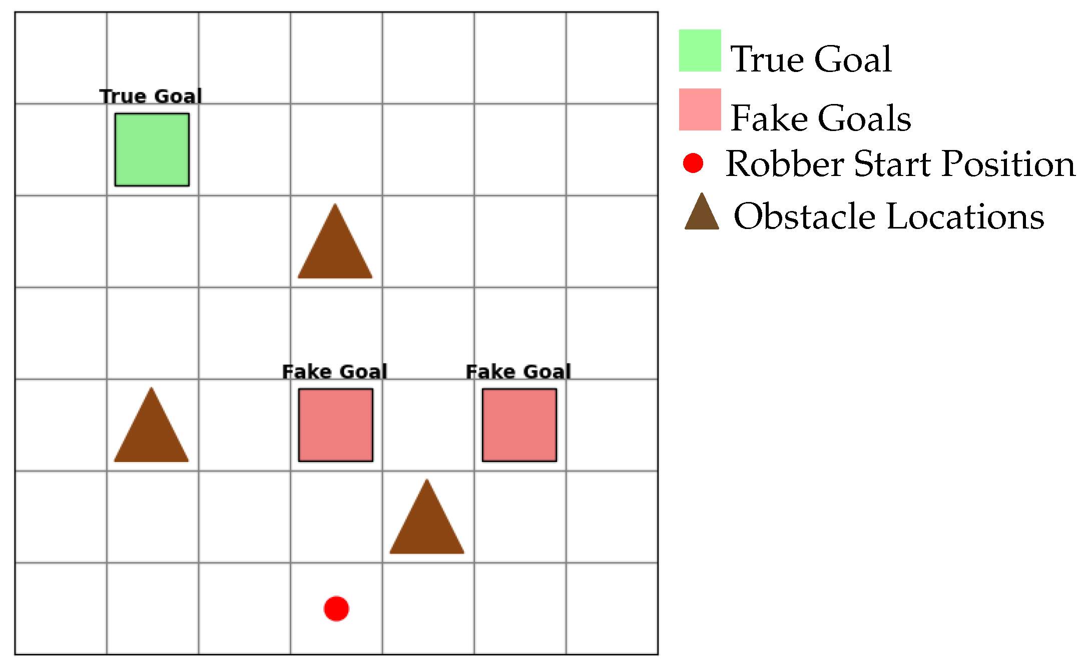
Our problem is motivated by a scenario in which a robber attempts to escape from a city. There are multiple exits from the city, but the robber has already selected a specific one (see
Figure 1). A police control room supervisor monitors the robber’s movements from a control room but does not know which exit the robber has chosen. The supervisor’s objective is to predict the robber’s selected exit and deploy reinforcements accordingly.
The supervisor has a limited number of reinforcement units available. At each time step, as the robber moves through the city, the supervisor deploys one unit of reinforcement to the exit that the supervisor currently believes the robber is heading toward. When the robber ultimately reaches the exit, the total reinforcement stationed at that location depends on two factors: the time elapsed until the robber’s arrival and the number of times the supervisor deployed reinforcements to that particular exit. This outcome captures the interaction between the robber’s path-selection strategy (which affects travel time) and the supervisor’s reinforcement-deployment strategy over time.
The abovementioned problem is a classical case of games with asymmetric information—the supervisor does not know the robber’s true exit choice, whereas the robber is aware of the supervisor’s uncertainty. The robber recognizes that he is being observed and that the supervisor’s strategy is influenced by his movements. Therefore, rather than proceed directly to his intended exit, he may initially move toward alternative exits to generate ambiguity. This misleading movement constitutes deception—it may cause the supervisor to misallocate resources and reinforce the incorrect exit (exaggeration can be a form of deception. However, naive exaggeration may prove detrimental to the agent rather than beneficial. For example, in our scenario, if the robber exaggerates excessively by taking too long to reach the exit, the supervisor may have sufficient time to reinforce the correct exit, even by allocating reinforcements randomly or uniformly across all exits). Meanwhile, the supervisor must infer the robber’s true intention from his ambiguous behavior and deploy reinforcements strategically—ideally predicting the correct exit despite the deception.
The objective of this article is to demonstrate how reinforcement learning, together with concepts from game theory, can be combined to learn deceptive strategies that leverage the information superiority of one agent over another.
2.2. Mathematical Formulation
We formulate the problem as a game on a discrete-time, grid-based environment defined over a finite two-dimensional lattice
of size
. Each cell
represents the robber’s possible location, with
and
. The environment comprises two learning agents—the
robber (
) and the
police officer (
)—and a set of
n goal locations
and a set of
k static obstacles
All goals lie in
free cells; that is,
. Exactly one goal is the
true goal, denoted
, and the remaining goals form the set of
fake goals,
(
Figure 2).
Let
denote the robber’s position at time
, and his action set is
For each goal
, let
denote the police reinforcement allocated at time
t, and define the police-reinforcement vector as
The police officer’s action set is denoted by
The environment is assumed to be deterministic: an action
moves the robber one cell in the chosen direction, and an action
updates the reinforcement vector by
We denote the state of the game at time
t by
which results in the state space being
. Let
be the robber’s policy, where
is the probability of selecting action
in state
, and let
be the police officer’s policy over
.
Define the terminal time to be the first instance when the robber reaches its true goal:
which depends on the policy pair
and the initial state
. The robber seeks to minimize the reinforcement at the true goal,
, while the police officer seeks to maximize it. In game-theoretic form, this objective can be expressed as
where the expectation is taken with respect to the randomization in the agents’ strategies.
This formulation differs from classical min–max games because the police officer does not know which goal is true and therefore cannot optimize directly. We employ reinforcement learning techniques for both and to learn their policies and . Our aim is to design reward structures so that can exploit its informational advantage to deceive , while learns counter-deception strategies to mitigate ’s deception.
2.3. Ambiguity and Strategic Trade-Offs
Ambiguity is the linchpin of effective deception. As long as the police officer cannot distinguish among multiple equally plausible goals, it must hedge, slowing its response and creating openings for the robber. Conversely, the robber must trade off path optimality against deceptive detours—too much ambiguity costs time, and too little increases the risk of exposing the true goal.
In this adversarial setting, the robber’s policy must balance
while the police officer’s policy must trade
By embedding these opposing objectives in a multi-agent reinforcement learning framework, we recover emergent equilibrium strategies that reflect both deception and counter-deception in complex, partially observed environments.
3. Game-Theoretic Reward Shaping
To foster rapid convergence and emergent strategic behavior, we enrich the baseline reinforcement-learning rewards with game-theoretic shaping terms that explicitly encode the adversarial structure of our multi-exit pursuit–evasion game. By penalizing or rewarding each agent according to both short-term navigation signals and inferred opponent intent, we bias exploration toward policies that exhibit robust deception (for the robber) or effective inference (for the police officer).
We borrow key concepts for the police officer-robber game from a related problem studied in [
26]. Due to the complexity of the problem—particularly with the inclusion of obstacles and multiple goals—theoretical analysis in [
26] is limited to obstacle-free grids with only one true goal and one decoy. Through our reward-shaping approach, we demonstrate that a deep Q-learning framework can successfully learn effective deception and counter-deception strategies in these more complex environments.
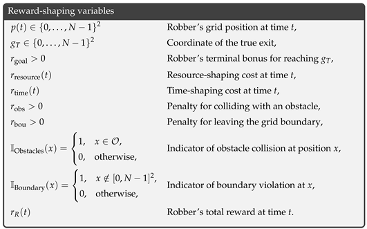
Before we present our detailed discussion on reward shaping, we summarize the key variables that will be used throughout this section in the frame below.
![Applsci 15 07805 i001]()
3.1. Robber Reward Shaping
We denote the robber’s per-step reward at time
t by
. Intuitively,
must serve three objectives simultaneously: (i) provide a strong incentive to reach the true exit, (ii) discourage invalid or aimless movements, and (iii) penalize lingering or predictable behavior that would make deception ineffective. More precisely, we consider the most recent resource allocation to the true goal for a time window of
H, i.e., the quantity
, where recall that
denotes
’s allocation to goal
i at time
t (for
, the window horizon is limited to
t). Using this allocation history, we define two reward-shaping quantities:
where
weighs how strongly past actions of
should penalize the Robber, and
controls the cost of delayed exit. That is, the longer
takes to reach the goal, the higher the penalty
. Notice that unlike most existing methods that assign a fixed pet-step cost (i.e.,
) to motivate a shorter path length, we consider a linearly increasing path length.
The final reward is computed as
where
is a large terminal bonus for reaching the goal,
and
penalize obstacle collisions or going out of the grid boundary, and the indicator functions activate only upon those events.
This formulation ensures that the robber is (i) strongly rewarded for successful escape, (ii) punished for reckless or non-progressing maneuvers, and (iii) discouraged from trajectories that allow the police officer to concentrate resources too heavily on the true exit too early.
3.2. Police Officer Reward Shaping
The police officer’s per-step reward,
, must encourage accurate inference of the robber’s hidden objective while maintaining coverage of alternative exits. We begin by measuring the change in (Manhattan) distance from the robber’s current position
to each exit
:
Notice that, due to the grid-world nature of the environment and the
up/down/left/right movement,
can only take one of the two values:
and 1. Therefore,
is a direct indicator of whether the robber moved closer to the goal
(i.e., when
) or moved further away. In general, one movement can lead to
being
for multiple goals. Therefore, to separate the goal(s) for which the distance was minimized by the robber, we define the set
’s allocation vector is then rewarded according to the following:
- ■
Unique Minimum: If with being the only goal in the set , we define ’s reward as
where
scales the incentive to concentrate force on the most likely exit. Notice that the allocation vector
satisfies the condition
as mentioned in (
1). Consequently,
in (
5) can equivalently be written as
This shows that at least half of the allocation must be assigned to the unique goal (i.e., ) for which the robber decreased its distance to receive a non-zero reward. If , the reward is negative, implying that the police officer is being penalized.
It should be noted that in our earlier formulation,
for each goal
i (see (
1)), which forces
to fully commit to the goal to receive a positive reward, as partial allocations are not permitted. To introduce exploration into
’s strategy, one could relax this constraint and allow fractional allocations, i.e.,
. While this adds flexibility to
’s strategy, it also increases the complexity of the problem, as
’s action space becomes continuous. Beyond this added complexity, such a formulation may be less practical, as in real-world settings,
may not be able to allocate arbitrary fractions of a unit to different goals. To strike a balance between practical applicability and strategic flexibility, we retain a discrete action space but expand the set of possible allocations beyond what was allowed in (
1). A detailed description of
will be provided later in the simulation section.
- ■
Tied Minima: If
, we refine the decision by introducing a new quantity
which denotes the sum of the current allocation at goal and the current distance to that goal. Essentially, represents the maximum possible amount of reinforcement that could be allocated to goal if it were the true goal, assuming that begins moving directly toward it and fully commits its resources to that goal for the remainder of the time. In our framework, is precisely the number of lattice steps needed to reach , and the police officer receives exactly one unit of reinforcement per time step. Consequently, both the distance and allocation terms are already expressed in identical, naturally normalized units. The unweighted sum therefore captures the total number of remaining allocation steps required to saturate goal i if the police officer were to devote all future resources there from time t onward. In other scenarios, one may need to use a weighted sum .
Let us define
and the set for which
’s are the lowest as follows
Now, using
, we define
’s reward as
encouraging the police officer to allocate proportionally among the most effective candidate goals. Finally, to penalize overcommitment to decoy exits, we grant a conservation bonus
whenever the robber has previously visited exit
i and the police officer allocates zero mass there. Collectively, these shaping terms drive the police officer to rapidly infer the robber’s intended exit, discourage wasteful dispersion of resources, and maintain a calibrated balance between exploration and exploitation in the allocation strategy.
The entire reward computation process is presented in Algorithm 1.
| Algorithm 1 One-Step Reward Computation |
| Require: robber_pos , goal_alloc , robber_action , police_action |
| 1: | |
| 2: | next_position(). | ▹ Robber’s next position |
| 3: | if
then |
| 4: | | |
| 5: | else if
then |
| 6: | | | ▹ Out of grid boundary penalty |
| 7: | else if
then |
| 8: | | | ▹ Obstacle collision penalty |
| 9: | else if
then |
| 10: | | | ▹ Non-movement penalty |
| 11: | end if |
| 12: | compute and | ▹ Equation (4) |
| 13: | | ▹ robber reward |
| 14: | for all . |
| 15: | Compute for all goals |
| 16: | |
| 17: | if
then |
| 18: | | let be the sole element of |
| 19: | | |
| 20: | else |
| 21: | | for each compute |
| 22: | | and |
| 23: | | for to n do |
| 24: | | | if then |
| 25: | | | | |
| 26: | | | else |
| 27: | | | | |
| 28: | | | end if |
| 29: | | | if the robber visited goal before and then |
| 30: | | | | | ▹ Police reward |
| 31: | | | end if |
| 32: | | end for |
| 33: | end if |
| 34: | return
|
4. Deep Q-Network Training
To jointly induce deceptive and counter-deceptive behaviors, we optimize the robber’s and police officer’s policies via deep Q-learning with soft target-network updates. Each agent maintains an online deep Q-network (DQN) and a lagging target DQN , both parametrized by multi-layer perceptrons with weights and , respectively. There are total of four networks (), two for each player.
Experience (in RL,
experience is a tuple that contains the current state, current action, reward, next state, and occasionally a binary variable denoting whether the episode ended in the next state or not) is stored in a replay buffer of symbolic capacity
C, from which minibatches of size
B are sampled to decorrelate updates. We employ a discount factor
, gradient-norm clipping bound
G, and a soft-update coefficient
so that after each gradient step the target parameters blend smoothly:
Exploration is governed by time-dependent rates : at each decision point an agent selects the action that maximizes its current Q-estimate with probability , and otherwise samples uniformly from its action set. The schedule for decaying is chosen to ensure ample early exploration followed by gradual consolidation on high-value strategies.
Updates proceed whenever the replay buffer contains at least
B transitions. A minibatch is drawn, and for each experience a bootstrapped target is computed against the target network using the
Huber loss to mitigate sensitivity to outliers. Gradients are clipped to norm
G before each parameter update, reinforcing stability in the non-stationary, adversarial training setting (Algorithm 2).
| Algorithm 2 Two-player DQN with Soft Target Updates |
| Require: replay capacity C, batch size B, discount , soft-update , grad-clip bound G |
| Ensure: trained Q-networks |
| 1: | Initialize online networks and targets and . |
| 2: | Initialize replay buffers with capacity C |
| 3: | for
do |
| 4: | | Observe game-states | ▹ Defined in Equation (2) |
| 5: | | Select via –greedy policies |
| 6: | | Execute ; observe | ▹done=1 iff |
| 7: | | Store transitions in |
| 8: | | if then |
| 9: | | | | ▹ Loss function for |
| 10: | | | Sample minibatch of size B from |
| 11: | | | for each experience in B do |
| 12: | | | | Compute targets |
| 13: | | | | | ▹ Huber Loss function for |
| 14: | | | end for |
| 15: | | | Update by minimizing ; clip gradients with bound G |
| 16: | | | | ▹ Target weight update |
| 17: | | end if |
| 18: | | if then |
| 19: | | | | ▹ Loss function for |
| 20: | | | Sample minibatch of size B from |
| 21: | | | for each experience in B do |
| 22: | | | | Compute targets |
| 23: | | | | | ▹ Huber Loss function for |
| 24: | | | end for |
| 25: | | | Update by minimizing ; clip gradients with bound G |
| 26: | | | | ▹ Target weight update |
| 27: | | end if |
| 28: | | Decay exploration rates |
| 29: | end for |
4.1. Neural Network Architectures for and
Each agent’s DQN maps a fixed-length feature vector into estimated Q-values over its discrete action set. Both the robber and the police officer use three fully connected hidden layers, but the robber’s network includes dropout for regularization whereas the police officer’s does not. The input and output dimensions differ according to each agent’s role, but the hidden-layer structure is otherwise identical in depth.
Overall Structure: Let
denote the input dimension (determined by the maximum number of goals
and obstacles
; see
Section 4.2) and let
denote the size of the agent’s action set (4 for the robber’s four movements;
for the police officer’s choice of goal). Then,
Robber’s network (
):
Here each “FC” is a fully connected layer, and each dropout layer uses probability .
Police officer’s network:
No dropout layers are inserted for the police network.
Figure 3 shows the robber’s DQN (with dropout), and
Figure 4 shows the police officer’s DQN (without dropout). Both diagrams are scaled to fit within typical journal margins.
To encourage the robber’s network to learn broadly generalizable deceptive strategies rather than memorizing specific exit configurations, we intersperse dropout layers after the first two hidden-layer activations. By randomly dropping a fraction of hidden units during training, the robber’s DQN is forced to distribute its internal representations across many pathways, reducing overfitting to particular grid layouts or goal placements and thus improving transfer to novel exit arrangements. The police officer’s network, in contrast, must develop highly precise value estimates to detect and counteract subtle deceptive cues; introducing dropout there tended to destabilize its ability to capture fine-grained distance–change and resource-allocation patterns. Empirically, we found that regularizing only the robber network strikes the right balance between robustness and sensitivity for our adversarial setting.
4.2. Input Feature Construction and Training Hyperparameters
This section provides a detailed explanation of how each environment state is encoded into a fixed-length feature vector, outlines the key training hyperparameters (including the exploration decay schedule), and explains why the same DQN architecture can seamlessly handle progressively increasingly complex scenarios. The input features to the DQNs vary depending on the game scenario. We categorize them into three groups: (1) games without obstacles, (2) games with obstacles, and (3) scenarios involving network generalization through dynamic goals and obstacles.
4.2.1. Games Without Obstacles
In this setup, the environment contains no obstacles. A special case within this scenario occurs when there are only two goals—one true and one decoy. For this case, analytical results are available in the game theory literature [
26]. This provides an opportunity to validate our results against a game-theoretic ground truth.
The current location of the robber, i.e.,
, and the current police allocation at the goals, i.e,
, are included as part of the feature vectors for both agents. In addition to that, the set of all exit locations
is also part of the inputs, where
denotes the grid coordinates of goal
. To incorporate knowledge about the true goal, we define an indicator vector associated with
:
This indicator vector is included only in the input to the robber’s network, , and not in the police’s network.
Therefore, the full feature set for the robber consists of:
with the dimension of the feature vector being
for a setup with
n goals. On the other hand, the full feature set for the police consists of
with the dimension of the feature vector being
.
This set-up will subsequently be used for Experiments 1 and 3 in our study.
4.2.2. Games with Obstacles
In addition to the input features mentioned in the previous case, we also include the relative distances to the obstacles
as features:
where, for all
,
denotes the relative distance vector from the robber’s current position to obstacle
. Consequently, in this case, the dimensions of the robber’s and police officer’s input features become
and
, respectively.
4.2.3. Network Generalization
In the previous two cases, training is conducted on fixed environments, where the number of goals, the number of obstacles, and the goal locations remain constant. To develop policies that generalize to different environments—and potentially to larger grids—we replace the absolute goal locations with relative distance vectors and distances to the goals. Consequently, the input feature dimensions for the robber and police networks are and , respectively. To accommodate a dynamic number of goals (up to N) and obstacles (up to K), we fix the input feature lengths to for the robber and for the police officer, applying a zero-padding scheme when the actual number of goals or obstacles is less than their respective maximums.
4.2.4. Training Hyperparameters
Both the robber’s and police officer’s DQNs are trained with off-policy Q-learning, using experience replay and a separate target network. The main hyperparameters are as follows:
Discount factor .
Adam optimizer with learning rate .
Replay buffer capacity , minibatch size .
Target network update: copy online parameters to target network every 50 episodes using soft policy update with
Exploration schedule (
-greedy):
After each episode, decays multiplicatively by , ensuring exploration does not fall below .
4.2.5. Computation Metrics
To assess the practical feasibility of our framework, we measured both time and space complexity on an NVIDIA RTX 2080 (8 GB VRAM, CUDA 11.8). Each experiment averages over 1000 episodes (training).
Training time. s per episode, including forward/back-prop and all environment interactions.
Inference latency. ms per decision step (batch size = 1).
Model size. 160 KB per DQN (32-bit weights), allowing the entire policy stack to reside comfortably in on-chip cache of low-power embedded boards.
Peak memory. 96 MB during training and 7 MB during inference, dominated by replay-buffer and tensor allocations, respectively.
These measurements demonstrate that our approach supports rapid prototyping, real-time control, and deployment on resource-constrained hardware without additional optimization.
5. Results and Simulations
We evaluate the performance of our deceptive and inference-driven policies across six canonical environments
Table 1. The primary metric reported in each setting is the Percentage of Fake-Goal Allocation (PFA), which measures the fraction of the police officer’s total reinforcement budget that is misallocated to fake exits, thereby quantifying the robber’s deception strength. All results reflect the mean over 10 independent runs with randomized goal placements.
- ■
Supplementary performance metrics: To provide a concise yet informative assessment of deception dynamics, we report three complementary quantities: the
Percentage of Fake-Exit Allocation (PFA), its derived
counter-deception score , and the
true-exit interception rate (TIR). PFA measures the fraction of the police officer’s total reinforcement budget that is misallocated to fake exits, thereby quantifying the robber’s deception strength. The counter-deception score inverts this value to give an immediate gauge of how effectively the police officer resists the lure. Finally, the interception rate captures the proportion of allocation steps that successfully cover the true exit, while a fake exit is active and can be written as
Together, these three metrics form a minimal “confusion-like” summary from which the full confusion-matrix entries (true/false positives and negatives) can be reconstructed when the total number of allocation steps is known. We focus on PFA as our primary metric and provide qualitative analysis of behavioral trends to highlight nuanced strategic patterns that emerge across different experimental conditions.
5.1. Experiment 1: Two-Goal Environment
In this baseline scenario—a
grid with one true and one decoy goal—the trained DQN police officer (
) dramatically reduces misallocation compared to naive strategies.
Table 2 reports the PFA, where
lowers the percentage of resources sent to the decoy by up to 40%.
The results demonstrate the effectiveness of our DQN-based approach compared to baseline strategies
Table 3. The trained DQN police officer (
) consistently outperforms the game-theoretic baseline (
), achieving identical or better performance across all robber policies. Notably,
maintains the same 28.57% PFA as
against the shortest-path (
), naive deceptive (
), and trained DQN (
) robbers while also handling the random robber (
) more effectively. The DQN robber (
) shows competitive performance against the baseline (
), achieving 28.57% PFA against
compared to
’s 25.00% against
, demonstrating that learned policies can match or exceed theoretical equilibrium strategies in practice.
The ablation study reveals the critical contribution of each component to our framework’s performance. The full MARL-DQN approach achieves the best performance with 28.6% PFA and 78% interception rate, significantly outperforming all ablated variants. Removing reward shaping degrades performance substantially (46.6% PFA, 62% interception), demonstrating that game-theoretic incentives are essential for learning effective deception strategies. The absence of intent inference also hurts performance (39.6% PFA, 68% interception), confirming that opponent modeling is crucial for counter-deception. Training on static layouts only results in the worst performance (53.6% PFA, 54% interception), highlighting the importance of dynamic environment training for generalization. These results validate that our integrated approach combining reward shaping, intent inference, and dynamic training is necessary for achieving robust deception and counter-deception capabilities.
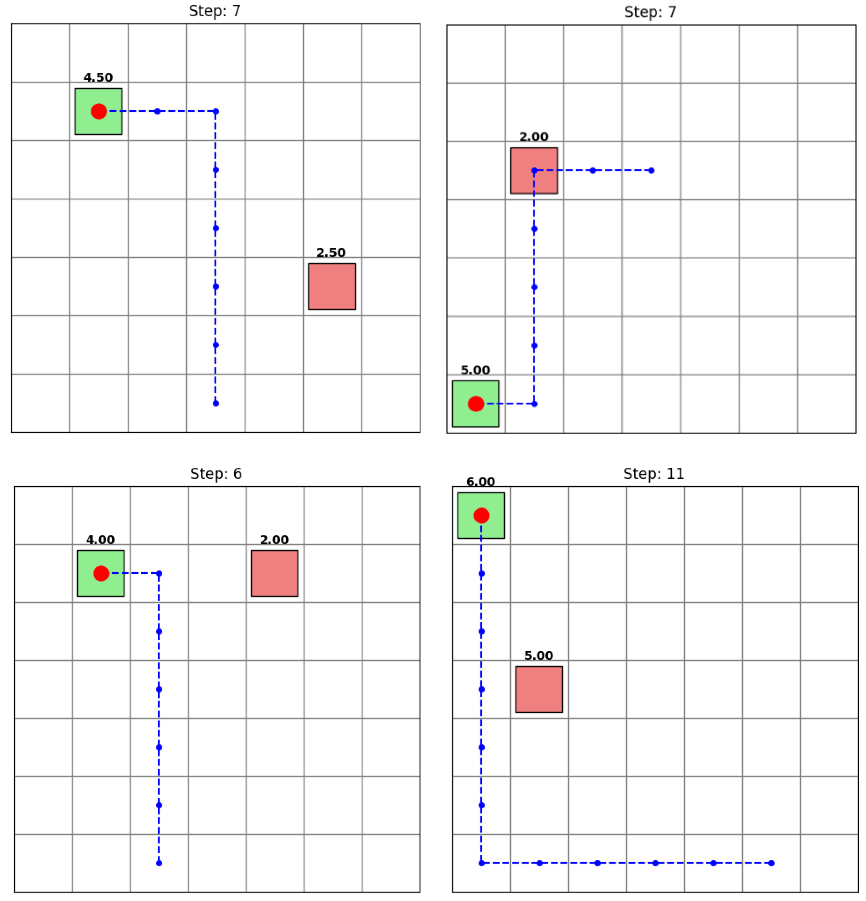
The results in
Figure 5 demonstrate that handcrafted and learned policies achieve more efficient, targeted deception compared to the indiscriminate strategy of
. Both the shortest-path robber (
) and the trained DQN robber (
) attain nearly the same deception rate, showing that strategic planning can be as effective as learned policies in simple scenarios.
5.2. Experiment 2: Two-Goal Environment with Obstacles
Introducing static obstacles increases navigational complexity. Despite this, the DQN police officer continues to outperform, as shown in
Table 4, demonstrating robust inference under spatial constraints.
Introducing obstacles significantly impacts each robber policy. The random () and shortest-path () strategies collide frequently with obstacles, causing early terminations and resulting in fake-goal percentages of 49.00% and 28.00%, respectively. The naive deceptive robber () initially detours toward a fake goal but lacks adaptive obstacle avoidance, yielding 40.00% PFA—a marginal improvement over non-learning policies.
By contrast, the trained DQN robber (
) learns to navigate around obstacles, achieving the highest fake-goal allocation (63.64%) under the random police and robust results (28.57%) against the DQN police. In cluttered environments, learning-based deception sustains longer trajectories and concentrates misdirection more effectively than static or random policies (
Figure 6). As complexity increases, online adaptation to obstacles proves essential for preserving high deception efficacy.
In the next three experiments, we evaluate the scalability and generalizability of our method by progressively increasing the complexity of the setup—starting with an increased number of goals (Experiment 5), followed by a greater number of obstacles (Experiment 6), and finally both in a dynamic scenario (Experiment 7).
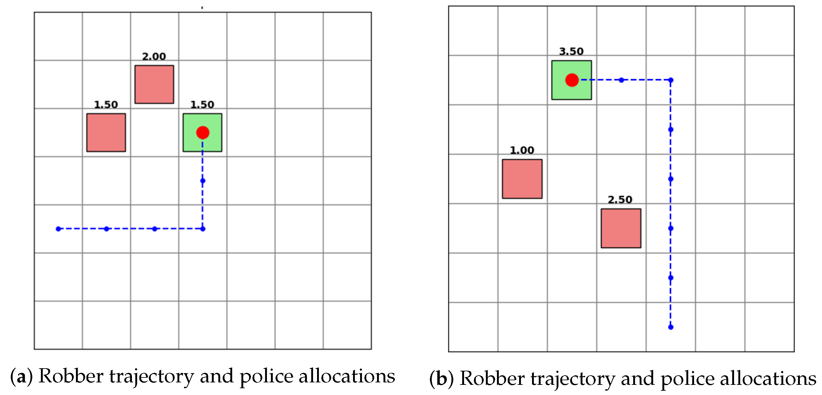
5.3. Experiment 3: Multi-Goal Environment
Scaling to three decoys on a
grid substantially increases goal ambiguity.
Table 5 shows that
maintains the lowest PFA, demonstrating its ability to minimize misallocation under higher uncertainty.
In the multi-goal environment, choosing among three decoys greatly amplifies deception complexity. The random robber (
) attains 76.47% fake-goal allocation—demonstrating exaggerated but inefficient deception. The shortest-path robber (
) reaches 64.29% PFA, offering sparse, unintended misdirection. The naive deceptive robber (
) achieves 76.00% PFA but still trails in efficiency. By contrast, the DQN robber (
) balances efficiency and efficacy: it secures 64.29% PFA (and 44.44% PFA against the DQN police). As decoy options increase, such targeted learning-based strategies are essential for maintaining high deception efficiency (
Figure 7).
5.4. Experiment 4: Multi-Goal Environment with Obstacles
Adding obstacles in the multi-goal grid further tests strategic inference. As
Table 6 shows,
retains superior performance, keeping PFA at its lowest levels.
In this experiment, non-learning policies (
) suffer frequent collisions that truncate their trajectories, yielding allocation rates varying from 75 to 87.5%. By contrast, the DQN-trained robber (
) learns to skirt obstacles, achieving 78.23–80.26% fake-goal allocation. This demonstrates that adaptive, learning-based strategies can sustain high deception efficiency in complex, cluttered settings(
Figure 8).
5.5. Experiment 5: Dynamic Goals (No Obstacles)
We broaden to 100 randomized trials on a
grid with dynamic exit placements. Even under non-stationary configurations, the trained police officer (
) consistently achieves the lowest average PFA (
Table 7).
In the dynamic goals environment, goal positions change each episode, requiring a single policy to adapt to all layouts(
Figure 9). The random robber (
) reaches 86.21% fake-goal allocation through indiscriminate behavior. The shortest-path (
) and naive deceptive (
) robbers achieve 60.14% and 69.00% PFA, respectively, but falter on novel configurations. In contrast, the DQN robber (
) generalizes across 100 layouts, securing 60.11% PFA and 40.34% against the adaptive DQN police officer—demonstrating true flexibility in dynamic settings.
At the same time, the DQN-trained police officer interprets distance change signals, resource allocation costs, and visitation history to infer the robber’s hidden goal more accurately than static or random policies. Across six environments, from two-goal grids to dynamic multi-goal layouts with obstacles, reduces the percentage of fake-goal allocation by up to fifty percent. This robust performance highlights the advantage of embedding opponent-aware shaping into the police officer’s learning process.
5.6. Experiment 6: Dynamic Goals with Obstacles
Finally, static obstacles are reintroduced in the dynamic setting.
Table 8 confirms that even under maximum complexity, the DQN police officer maintains robust performance, minimizing PFA.
Although the random robber (
) records 88.23% fake-goal allocation under the random police officer, obstacle collisions restrict its effectiveness, revealing its deception as indiscriminate. The shortest-path robber (
) achieves 66.00% but lacks adaptive avoidance. In contrast, the DQN robber (
) deliberately navigates around obstacles, securing 70.26%, demonstrating genuine strategic adaptation (
Figure 10).
6. Discussion
Our experiments demonstrate that game-theoretic reward shaping produces sophisticated strategic behaviors in both agents. The DQN-trained robber learns to orchestrate decoy visits with remarkable precision, inducing costly misallocations by the police officer while avoiding unnecessary detours and obstacle penalties. In cluttered grids naive deceptive heuristics often become trapped, whereas maintains efficiency without sacrificing strategic ambiguity.
At the same time the DQN-trained police officer interprets distance change signals, resource allocation costs, and visitation history to infer the robber’s hidden goal more accurately than static or random policies. Across six environments, from two-goal grids to dynamic multi-goal layouts with obstacles, reduces the percentage of fake-goal allocation by up to fifty percent and minimizes wasted visits to decoys. This robust performance highlights the advantage of embedding opponent-aware shaping into the police officer’s learning process.
These results show that deception and counter deception emerge naturally when reward functions reflect core principles of pursuit evasion and signaling games. Furthermore the learned policies generalize to novel layouts and goal configurations, suggesting that our shaping terms capture fundamental adversarial structure rather than overfitting to specific maps. In this way our framework bridges classical theory and deep reinforcement learning, opening new pathways for strategic planning under uncertainty.
7. Conclusions
We have introduced a game-theoretic reward-shaping framework that integrates opponent aware incentives into multi-agent deep Q-learning. By augmenting standard rewards with distance change feedback, resource allocation cost, and history aware bonuses, our method enables decentralized policies capable of both deception and counter-deception under partial observability and physical constraints.
Empirical evaluation across six progressively complex grid world scenarios from simple two-goal arenas to dynamic multi-goal environments with obstacles confirms that shaped DQN agents consistently outperform naive baselines. The shaped robber orchestrates precise decoy visits to maximize misdirection, while the shaped police officer anticipates and counters those signals, achieving up to fifty percent reduction in misallocation. Both agents maintain strong performance under dynamic goal relocations and navigational challenges.
Future work will advance three directions to accelerate learning and broaden applicability. First, integrating a policy space response oracles meta solver will equip agents to adapt to mixed strategy equilibria and resilient adversaries. Second, curriculum learning schedules that gradually increase environment complexity can speed convergence and enhance generalization. Third, extending the state representation with graph-based node embeddings will enable deployment in real world map scenarios, such as traffic flow management, transportation logistics, military interception planning, and autonomous surveillance on road networks. These extensions promise to translate our strategic reward-shaping paradigm from grid-world benchmarks to high-impact applications in security and infrastructure.
Author Contributions
Conceptualization, D.M.; methodology, S.K.R.M. and D.M.; software, S.K.R.M.; validation, S.K.R.M.; formal analysis, S.K.R.M.; investigation, S.K.R.M.; resources, D.M.; data curation, S.K.R.M.; writing—original draft preparation, S.K.R.M. and D.M.; writing—review and editing, D.M.; visualization, S.K.R.M.; supervision, D.M.; project administration, D.M.; funding acquisition, D.M. All authors have read and agreed to the published version of the manuscript.
Funding
This research is supported by the ARL grant ARL DCIST CRA W911NF-17-2-0181.
Institutional Review Board Statement
Not applicable.
Informed Consent Statement
Not applicable.
Data Availability Statement
The raw data supporting the conclusions of this article will be made available by the authors on request.
Conflicts of Interest
The authors declare no conflicts of interest.
References
- Hyman, R. The psychology of deception. Annu. Rev. Psychol. 1989, 40, 133–154. [Google Scholar] [CrossRef]
- Carson, T.L. Lying and Deception: Theory and Practice; Oxford University Press: Oxford, UK, 2010. [Google Scholar]
- Chelliah, J.; Swamy, Y. Deception and lies in business strategy. J. Bus. Strategy 2018, 39, 36–42. [Google Scholar] [CrossRef]
- Maithripala, D.H.A.; Jayasuriya, S. Radar deception through phantom track generation. In Proceedings of the American Control Conference, Portland, OR, USA, 8–10 June 2005; pp. 4102–4106. [Google Scholar]
- Ko, K.; Kim, S.; Kwon, H. Selective Audio Perturbations for Targeting Specific Phrases in Speech Recognition Systems. Int. J. Comput. Intell. Syst. 2025, 18, 103. [Google Scholar] [CrossRef]
- Root, P.; De Mot, J.; Feron, E. Randomized path planning with deceptive strategies. In Proceedings of the American Control Conference, Portland, OR, USA, 8–10 June 2005; pp. 1551–1556. [Google Scholar]
- Hespanha, J.P.; Ateskan, Y.S.; Kizilocak, H. Deception in non-cooperative games with partial information. In Proceedings of the 2nd DARPA-JFACC Symposium on Advances in Enterprise Control, Minneapolis, MN, USA, 10–11 July 2000. [Google Scholar]
- Chen, S.; Savas, Y.; Karabag, M.O.; Sadler, B.M.; Topcu, U. Deceptive planning for resource allocation. In Proceedings of the 2024 American Control Conference (ACC), Toronto, ON, Canada, 10–12 July 2024; pp. 4188–4195. [Google Scholar]
- Kiely, M.; Ahiskali, M.; Borde, E.; Bowman, B.; Bowman, D.; Van Bruggen, D.; Cowan, K.C.; Dasgupta, P.; Devendorf, E.; Edwards, B.; et al. Exploring the Efficacy of Multi-Agent Reinforcement Learning for Autonomous Cyber Defence: A CAGE Challenge 4 Perspective. In Proceedings of the AAAI Conference on Artificial Intelligence, Philadelphia, PA, USA, 25 February–4 March 2025; Volume 39, pp. 28907–28913. [Google Scholar]
- Whaley, B. Toward a general theory of deception. J. Strateg. Stud. 1982, 5, 178–192. [Google Scholar] [CrossRef]
- Liang, J.; Miao, H.; Li, K.; Tan, J.; Wang, X.; Luo, R.; Jiang, Y. A Review of Multi-Agent Reinforcement Learning Algorithms. Electronics 2025, 14, 820. [Google Scholar] [CrossRef]
- Chelarescu, P. Deception in Social Learning: A Multi-Agent Reinforcement Learning Perspective. arXiv 2021, arXiv:2106.05402. [Google Scholar]
- McEneaney, W.; Singh, R. Deception in autonomous vehicle decision making in an adversarial environment. In Proceedings of the AIAA Guidance, Navigation, and Control Conference and Exhibit, San Francisco, CA, USA, 15 August–18 August 2005; p. 6152. [Google Scholar]
- Huang, Y.; Zhu, Q. A pursuit-evasion differential game with strategic information acquisition. arXiv 2021, arXiv:2102.05469. [Google Scholar]
- Sayin, M.; Zhang, K.; Leslie, D.; Basar, T.; Ozdaglar, A. Decentralized Q-learning in zero-sum Markov games. Adv. Neural Inf. Process. Syst. 2021, 34, 18320–18334. [Google Scholar]
- Huang, L.; Zhu, Q. A dynamic game framework for rational and persistent robot deception with an application to deceptive pursuit-evasion. IEEE Trans. Autom. Sci. Eng. 2021, 19, 2918–2932. [Google Scholar] [CrossRef]
- Fatemi, M.Y.; Suttle, W.A.; Sadler, B.M. Deceptive path planning via reinforcement learning with graph neural networks. arXiv 2024, arXiv:2402.06552. [Google Scholar]
- Wong, A.; Bäck, T.; Kononova, A.V.; Plaat, A. Deep multiagent reinforcement learning: Challenges and directions. Artif. Intell. Rev. 2023, 56, 5023–5056. [Google Scholar] [CrossRef]
- Zhou, B. Reinforcement Learning for Impartial Games and Complex Combinatorial Optimisation Problems. Available online: https://qmro.qmul.ac.uk/xmlui/handle/123456789/96718 (accessed on 26 June 2025).
- Dao, T.K.; Ngo, T.G.; Pan, J.S.; Nguyen, T.T.T.; Nguyen, T.T. Enhancing Path Planning Capabilities of Automated Guided Vehicles in Dynamic Environments: Multi-Objective PSO and Dynamic-Window Approach. Biomimetics 2024, 9, 35. [Google Scholar] [CrossRef] [PubMed]
- Lowe, R.; Wu, Y.; Tamar, A.; Harb, J.; Abbeel, P.; Mordatch, I. Multi-agent actor-critic for mixed cooperative-competitive environments. Adv. Neural Inf. Process. Syst. 2017, 30. Available online: https://proceedings.neurips.cc/paper_files/paper/2017/file/68a9750337a418a86fe06c1991a1d64c-Paper.pdf (accessed on 26 June 2025).
- Shoham, Y.; Leyton-Brown, K. Multiagent Systems: Algorithmic, Game-Theoretic, and Logical Foundations; Cambridge University Press: Cambridge, UK, 2008. [Google Scholar]
- Hu, J.; Wellman, M.P. Nash Q-learning for general-sum stochastic games. J. Mach. Learn. Res. 2003, 4, 1039–1069. [Google Scholar]
- Wu, B.; Cubuktepe, M.; Bharadwaj, S.; Topcu, U. Reward-based deception with cognitive bias. In Proceedings of the 58th Conference on Decision and Control, Nice, France, 11–13 December 2019; pp. 2265–2270. [Google Scholar]
- Jain, G.; Kumar, A.; Bhat, S.A. Recent developments of game theory and reinforcement learning approaches: A systematic review. IEEE Access 2024, 12, 9999–10011. [Google Scholar] [CrossRef]
- Rostobaya, V.; Guan, Y.; Berneburg, J.; Dorothy, M.; Shishika, D. Deception by Motion: The Eater and the Mover Game. IEEE Control Syst. Lett. 2023, 7, 3157–3162. [Google Scholar] [CrossRef]
- Patil, A.; Karabag, M.O.; Tanaka, T.; Topcu, U. Simulator-driven deceptive control via path integral approach. In Proceedings of the 62nd IEEE Conference on Decision and Control, Singapore, 13–15 December 2023; pp. 271–277. [Google Scholar]
- Fu, J. On almost-sure intention deception planning that exploits imperfect observers. In Proceedings of the International Conference on Decision and Game Theory for Security, PIttsburgh, PA, USA, 26–28 October 2022; Springer: Berlin, Germany, 2022; pp. 67–86. [Google Scholar]
- Shishika, D.; Von Moll, A.; Maity, D.; Dorothy, M. Deception in differential games: Information limiting strategy to induce dilemma. arXiv 2024, arXiv:2405.07465. [Google Scholar]
- Casgrain, P.; Ning, B.; Jaimungal, S. Deep Q-learning for Nash equilibria: Nash-DQN. Appl. Math. Financ. 2022, 29, 62–78. [Google Scholar] [CrossRef]
- Waseem, M.; Chang, Q. From Nash Q-learning to Nash-MADDPG: Advancements in multiagent control for multiproduct flexible manufacturing systems. J. Manuf. Syst. 2024, 74, 129–140. [Google Scholar] [CrossRef]
Figure 1.
Schematic of the game where the police officer does not know the exit the robber is going to use to leave the city.
Figure 1.
Schematic of the game where the police officer does not know the exit the robber is going to use to leave the city.
Figure 2.
Sample environment with multiple goals and obstacles.
Figure 2.
Sample environment with multiple goals and obstacles.
Figure 3.
Robber’s DQN architecture with dropout layers. The input dimension depends on and . After each of the first two ReLU activations, a dropout layer with probability is applied.
Figure 3.
Robber’s DQN architecture with dropout layers. The input dimension depends on and . After each of the first two ReLU activations, a dropout layer with probability is applied.
Figure 4.
Police officer’s DQN architecture without dropout. The input dimension depends on and ; output dimension .
Figure 4.
Police officer’s DQN architecture without dropout. The input dimension depends on and ; output dimension .
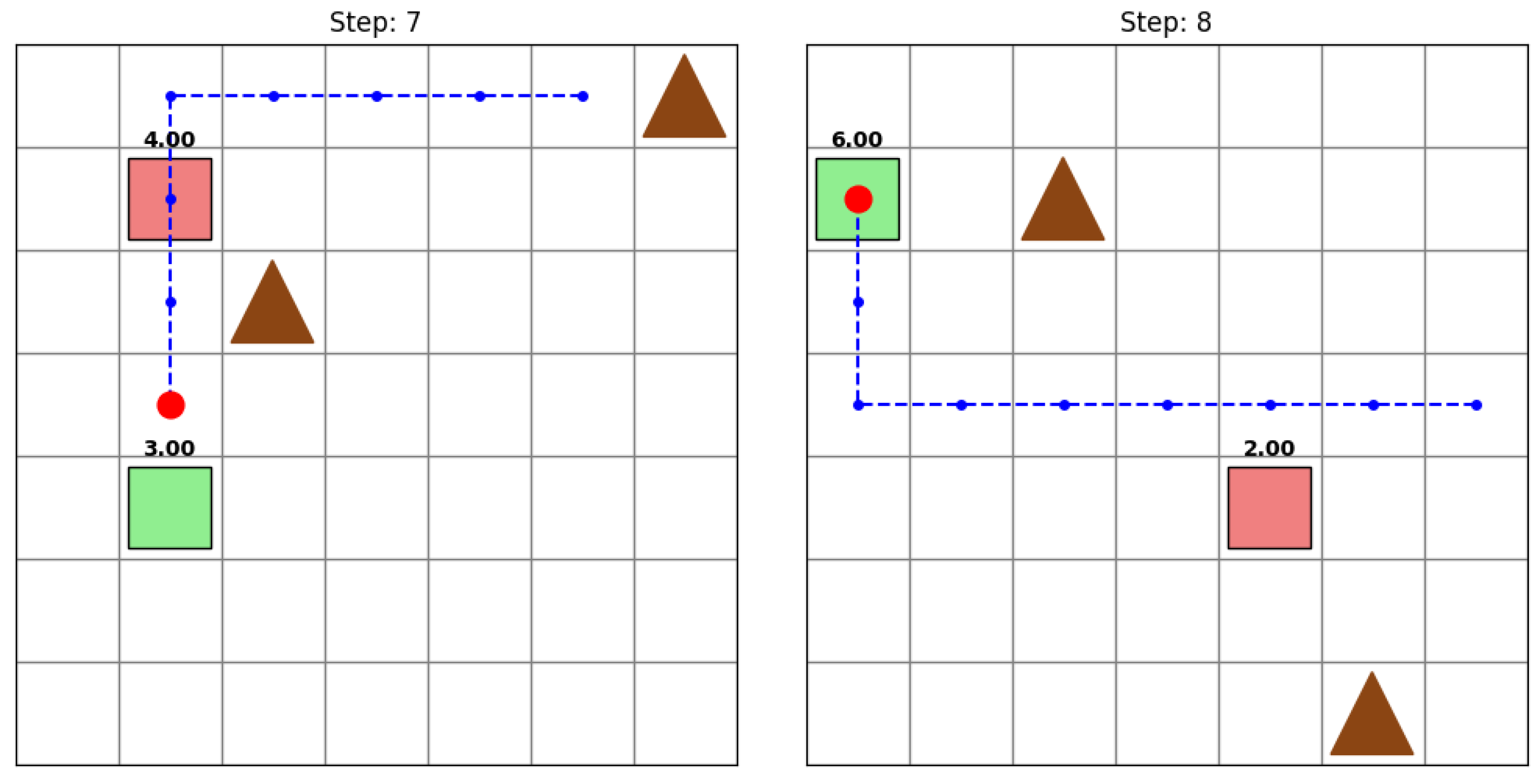
Figure 5.
Four simulation trial runs with four different true/fake exit configurations. The blue dotted line traces the robber’s path; numbers above each exit indicate resources allocated by the police officer, with green shading marking the true goal and red shading marking decoy goals. The ‘step’ numbers above each plot denotes , i.e., the number of steps it took the robber to reach its true exit.
Figure 6.
Simulation trial showing the robber’s path (blue dotted line); numbers above each exit indicate police resource allocations. True goals are shaded green, decoy goals red.
Figure 6.
Simulation trial showing the robber’s path (blue dotted line); numbers above each exit indicate police resource allocations. True goals are shaded green, decoy goals red.
Figure 7.
The blue dotted line traces the robber’s path; numbers above each exit indicate resources allocated by the police officer, with green shading marking the true goal and red shading marking decoy goals.
Figure 7.
The blue dotted line traces the robber’s path; numbers above each exit indicate resources allocated by the police officer, with green shading marking the true goal and red shading marking decoy goals.
Figure 8.
The blue dotted line traces the robber’s path; numbers above each exit indicate police resource allocations. True goals are shaded green, and decoy goals are shaded red.
Figure 8.
The blue dotted line traces the robber’s path; numbers above each exit indicate police resource allocations. True goals are shaded green, and decoy goals are shaded red.
Figure 9.
Simulation snapshots from the trained model in dynamic environments with varying goal configurations. The blue dotted line shows the robber’s trajectory, and the number above each goal indicates police resource allocation.
Figure 9.
Simulation snapshots from the trained model in dynamic environments with varying goal configurations. The blue dotted line shows the robber’s trajectory, and the number above each goal indicates police resource allocation.
Figure 10.
Simulation snapshots from the trained model in dynamic environments with varied goals. The blue dotted line represents the robber’s trajectory, and the number above each goal indicates the resources allocated by the police officer.
Figure 10.
Simulation snapshots from the trained model in dynamic environments with varied goals. The blue dotted line represents the robber’s trajectory, and the number above each goal indicates the resources allocated by the police officer.
Table 1.
Policy abbreviations and descriptions.
Table 1.
Policy abbreviations and descriptions.
| Abbreviation | Description |
|---|
| Random Robber: moves chosen uniformly at random. |
| Shortest-Path Robber: greedily minimizes Manhattan distance to the true exit. |
| Naïve Deceptive Robber: visits one decoy then proceeds to the true exit. |
| Trained DQN Robber: learns deceptive trajectories via deep Q-learning. |
| Baseline Game-Theoretic Robber: follows the Stackelberg deception equilibrium strategy from [26]. |
| Random Police Officer: allocates resources uniformly at random. |
| Fully Informed Police Officer: all resources are allocated to the true exit. |
| Trained DQN Police Officer: learns to infer intent and counter deception via deep Q-learning. |
| Baseline Game-Theoretic Police Officer: allocates according to the equilibrium strategy from [26]. |
Table 2.
PFA (%) in the two-goal environment.
Table 2.
PFA (%) in the two-goal environment.
| | | ’s Policy |
| | | | | | |
| ’s Policy | | 52.00 | 0.00 | 52.00 | 48.00 |
| 46.00 | 0.00 | 28.57 | 24.50 |
| 52.00 | 0.00 | 34.00 | 32.00 |
| 38.89 | 0.00 | 28.57 | 26.00 |
| 46.00 | 0.00 | 28.57 | 25.00 |
Table 3.
Ablation study in the two-goal environment (Experiment 1). Percentage of fake-goal allocation (PFA) and true-exit interception rate for different model variants. Lower PFA and higher interception are better.
Table 3.
Ablation study in the two-goal environment (Experiment 1). Percentage of fake-goal allocation (PFA) and true-exit interception rate for different model variants. Lower PFA and higher interception are better.
| Variant | PFA (%) | Interception Rate (%) |
|---|
| Full MARL-DQN (ours) | 28.6 | 78 |
| No reward shaping | 46.6 | 62 |
| No intent inference | 39.6 | 68 |
| Static layout only | 53.6 | 54 |
Table 4.
PFA (%) with obstacles in the two-goal environment.
Table 4.
PFA (%) with obstacles in the two-goal environment.
| | | ’s Policy |
| | | | | |
| ’s Policy | | 49.00 | 0.00 | 35.00 |
| 28.00 | 0.00 | 32.00 |
| 40.00 | 0.00 | 36.00 |
| 63.64 | 0.00 | 28.57 |
Table 5.
PFA (%) in the multi-goal environment.
Table 5.
PFA (%) in the multi-goal environment.
| | | ’s Policy |
| | | | | |
| ’s Policy | | 76.47 | 0.00 | 75.00 |
| 64.29 | 0.00 | 57.14 |
| 76.00 | 0.00 | 66.00 |
| 64.29 | 0.00 | 44.44 |
Table 6.
PFA (%) with obstacles in the multi-goal environment.
Table 6.
PFA (%) with obstacles in the multi-goal environment.
| | | ’s Policy |
| | | | | |
| ’s Policy | | 87.50 | 0.00 | 75.00 |
| 75.00 | 0.00 | 57.14 |
| 78.50 | 0.00 | 80.50 |
| 80.26 | 0.00 | 78.23 |
Table 7.
PFA (%) for dynamic goals (no obstacles).
Table 7.
PFA (%) for dynamic goals (no obstacles).
| | | ’s Policy |
| | | | | |
| ’s Policy | | 86.21 | 0.00 | 85.00 |
| 60.14 | 0.00 | 53.12 |
| 69.00 | 0.00 | 64.00 |
| 60.11 | 0.00 | 40.34 |
Table 8.
PFA (%) for dynamic goals with obstacles.
Table 8.
PFA (%) for dynamic goals with obstacles.
| | | ’s Policy |
| | | | | |
| ’s Policy | | 88.23 | 0.00 | 72.20 |
| 66.00 | 0.00 | 52.76 |
| 72.62 | 0.00 | 60.22 |
| 70.26 | 0.00 | 72.25 |
| Disclaimer/Publisher’s Note: The statements, opinions and data contained in all publications are solely those of the individual author(s) and contributor(s) and not of MDPI and/or the editor(s). MDPI and/or the editor(s) disclaim responsibility for any injury to people or property resulting from any ideas, methods, instructions or products referred to in the content. |
© 2025 by the authors. Licensee MDPI, Basel, Switzerland. This article is an open access article distributed under the terms and conditions of the Creative Commons Attribution (CC BY) license (https://creativecommons.org/licenses/by/4.0/).


