Article

Numerical Simulation and Analysis of Heart–Aorta Fluid–Structure Interaction Based on S-ALE Method

School of Mechanical & Automotive Engineering, South China University of Technology, Guangzhou 510641, China
*
Author to whom correspondence should be addressed.
Appl. Sci. 2025, 15(14), 7769; https://doi.org/10.3390/app15147769
Submission received: 17 May 2025 / Revised: 6 July 2025 / Accepted: 9 July 2025 / Published: 10 July 2025

Abstract

The aim of this study is to understand the hemodynamic responses in the heart–aorta system under physiological states and use this understanding to enhance the hemodynamic response analysis of cardiovascular fluid–structure interaction (FSI) models. This article developed a heart–aorta FSI model by constructing a structured fluid domain using the S-ALE method. The model realized a cardiac blood pumping pattern by applying a time-varying displacement load to the left ventricle (LV). The simulation reliability of the model was effectively verified by comparing the hemodynamic responses to the literature data. The FSI analysis in different physiological states showed that the altered ejection volume due to changes in LV systole displacement was a key factor influencing the hemodynamic response. As LV systole displacement increased, blood velocity, flow rate, and wall shear stress (WSS) showed a significant linear increase. The effect of changes in blood viscosity on the WSS demonstrated a significant linear correlation. However, the effect on blood velocity and flow rate did not present any significant difference. The S-ALE method used in this paper can rapidly generate fluid domains, providing technical support for the development of personalized medicine in the cardiovascular field.

1. Introduction

Cardiovascular disease is one of the leading causes of death worldwide, and the pathogenesis of aortic diseases (such as aortic dissection and aneurysms) is closely related to hemodynamic factors [1,2]. The heart and aorta form a complex FSI system, and the interaction between blood flow and the vessel wall directly affects the mechanical response of the vessel and the pathological development. Traditional medical imaging techniques, e.g., ultrasound, computed tomography (CT), and cardiovascular magnetic resonance (CMR) can provide basic information about blood flow and vascular morphology, but they are unable to accurately quantify hemodynamic parameters such as WSS and pressure distribution and cannot directly reflect the dynamic deformation process of the vascular wall [3,4]. Therefore, numerical simulation analysis has become an important research method for effectively reflecting hemodynamic responses under physiological states.
In recent years, the integration of computational fluid dynamics (CFD) and the finite element method (FEM) has provided an effective approach for FSI simulations [5,6,7]. However, conventional CFD-FEM coupling methods face challenges such as mesh distortion and poor computational stability when dealing with large deformation problems (e.g., pulsatile expansion of the aorta) [8]. The Arbitrary Lagrangian–Eulerian (ALE) method has been widely adopted in cardiovascular FSI simulations due to its ability to effectively balance the Eulerian description of the fluid domain and the Lagrangian description of the structure domain, making it suitable for large deformation FSI problems [9]. The Structured-ALE (S-ALE) method is based on the ALE method and incorporates structured meshes and adaptive technology to effectively improve the computational stability of large deformation problems. This methodology has been successfully validated in impact mechanics, particularly in ship engineering applications [10,11]. However, its application in biomedical engineering, particularly for heart–aorta FSI simulations, remains an area requiring further exploration.
The hemodynamics of the vascular system is a complex physiological process. The dynamic mechanical loads generated by periodic pulsatile blood flow can affect the tissue structure of the vascular wall, thereby inducing various vascular diseases. To investigate the FSI action mechanisms between blood flow and vascular walls, scholars have developed a variety of research methods and made significant progress [12,13,14,15]. However, due to computational efficiency considerations, some studies typically model only local regions of the blood vessels [16,17] or even use idealized structural models to simplify the analysis [18,19]. For example, Issakhov et al. [20] employed an idealized thin-walled cylindrical model to simplify the geometric characteristics of real blood vessels when conducting a comparative analysis of the effects of arterial wall structure on hemodynamics and vascular deformation in normal and stenotic states. However, the reliability of this model was lacked sufficient experimental or clinical data validation. In terms of fluid domain modeling, Taheri et al. [21] used the smooth particle hydrodynamics (SPH) method to discretize blood components. However, due to computational efficiency limitations, each particle only represented the average characteristics of the blood components and could not accurately reflect the continuity of real blood flow. Although the ALE method is widely used in blood-related FSI analysis, its fluid domain modeling is highly dependent on high-quality hexahedral meshes [22,23,24]. During the preliminary modeling phase, a significant amount of time is often required for mesh generation. In order to obtain a high-quality mesh, it is usually necessary to simplify the geometry of the model, which can affect the accuracy of the simulation to a certain extent. Compared to the ALE method, the S-ALE method combines structured meshes with adaptive technology, not only achieving efficient fluid domain modeling, but also significantly improving computational efficiency [10,11].
When simulating blood FSI under physiological states, existing studies typically use the time-varying blood velocity curve as the boundary condition for the vessel inlet [12,13,15,16,20,25]. However, relevant studies have shown that the distribution of blood flow velocity on vascular cross-sections exhibits significant non-uniformity [20,23]. Using only a single velocity–time curve as a boundary condition is insufficient to reflect the complex hemodynamic characteristics under physiological states. Here, a displacement–time load boundary condition is employed to simulate the periodic systolic and diastolic movement of the left ventricle, thus more realistically reproducing the process of heart pumping.
In this work, a numerical simulation analysis of the heart–aorta FSI under physiological states was conducted using the LS-DYNA explicit dynamics solver based on the S-ALE method. Through a comparative validation against the existing literature data, the applicability and reliability of the S-ALE method for simulating FSI problems in complex cardiovascular systems were confirmed. Based on the validated model, a preliminary application analysis of the heart–aorta FSI under different physiological states was performed.

2. Materials and Methods

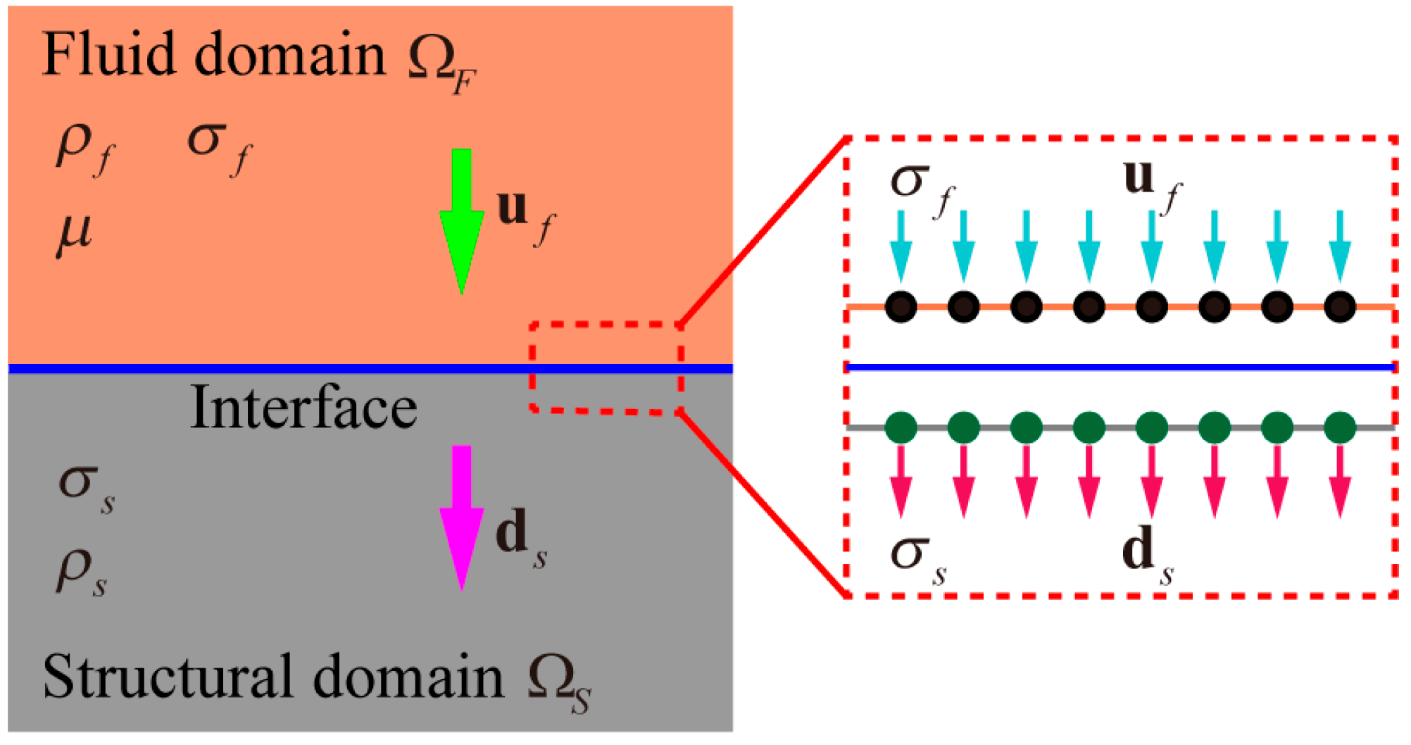
2.1. S-ALE Method Fundamentals and Coupling Conditions

The S-ALE method is an advanced FSI simulation that combines the structured fluid domain with the ALE algorithm, which enables the FSI analysis of structures in large deformations. “Structured” refers to an orthogonal fluid domain mesh created using an adaptive method. The ALE algorithm has the advantages of the Lagrangian and Eulerian algorithms. Figure 1 is a schematic diagram of the principle of FSI. The Navier–Stokes equations are used in the fluid domain, which are expressed as follows.
Conservation of mass equation:
ρ f t + ( ρ f u f ) = 0
where ρ f is the fluid density and u f is the fluid velocity.
Conservation of momentum equation:
( ρ f u f ) t + ( ρ f u f u f ) = p + σ f + f f
where p is the fluid pressure, σ f is the fluid viscous stress tensor, and f f is the fluid body force.
Conservation of energy equation:
( ρ f E ) t + ( ρ f E u f ) = ( p u f ) + ( σ f u f ) + f f u f
here, E is the total energy per unit mass.
For the case where the fluid density ρ f maintains a constant value throughout the formulation (i.e., ρ f / t = 0 and ρ f = 0 ), the governing equations characterize incompressible flow conditions.
The governing equation of the structural domain is based on the momentum conservation equation of solid mechanics, as shown in formula 4:
ρ s 2 d s t 2 = σ s + f s
where ρ s is the structural density, d s is the structural displacement, σ s is the structural stress tensor, and f s is the structural body force.
In FSI systems, fluid forces act on the interface of the structure and affect its motion, while the motion of the structure causes changes in the fluid computational domain and boundary conditions, thereby affecting the flow field. The coupling interface between the fluid domain and the structural domain needs to meet the following conditions.
Velocity continuity:
u f = d s t
Stress equilibrium:
σ f n = σ s n
where n is the interface normal vector.

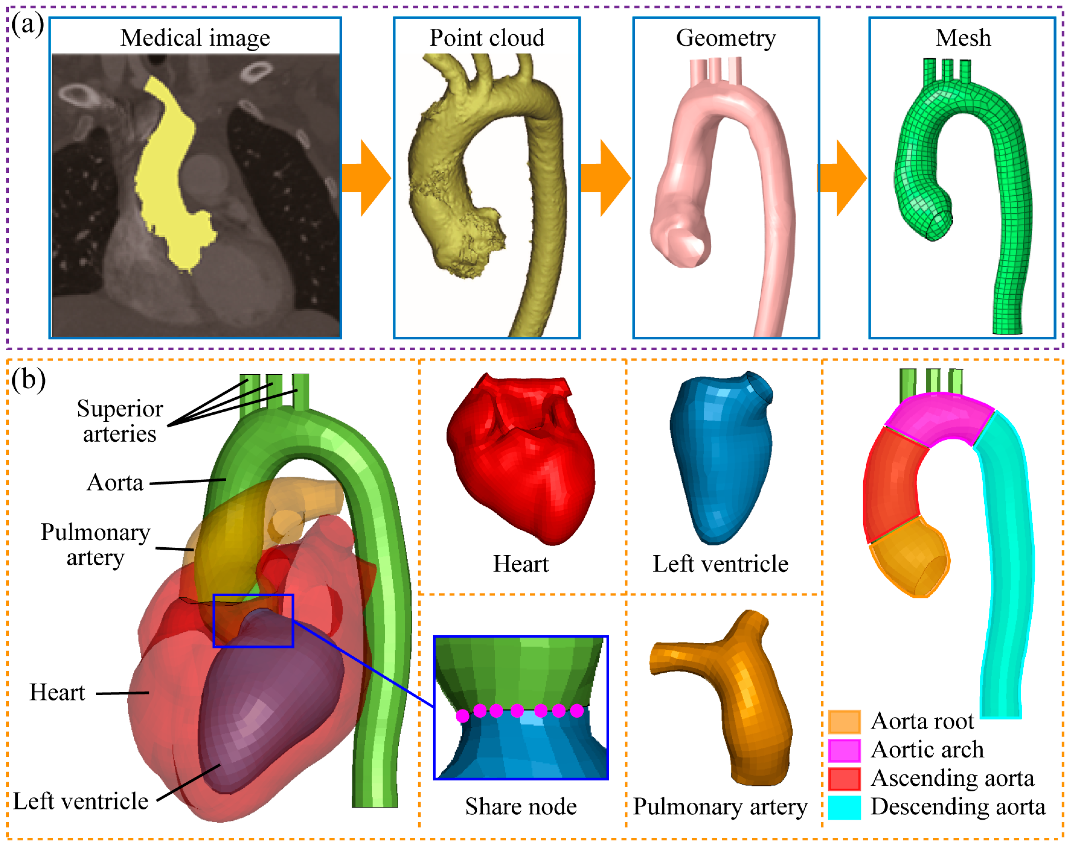
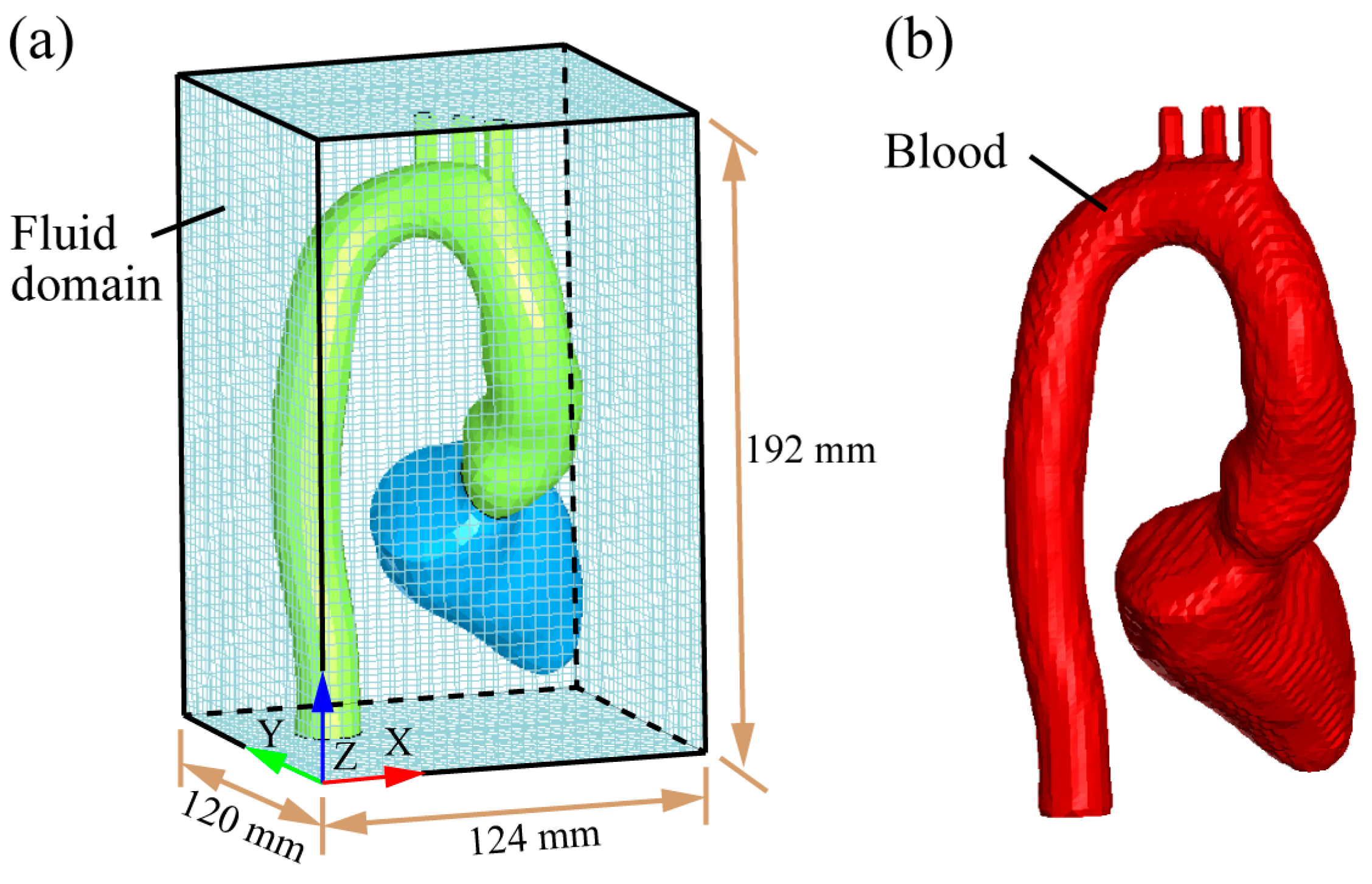
2.2. Establishment of Heart–Aorta FSI Model

The heart–aorta finite element model used in the study was established from previous computed tomography scans [26]. The model was developed through 3D reconstruction technology to obtain detailed anatomical structural features, as shown in Figure 2. Taking the aorta as an example (Figure 2a), Mimics 10.0 (Materialize Inc., Leuven, Belgium) was used to extract the point cloud from the CT image data. Then, the point cloud data were imported into Geomagic Studio 12 (3D Systems Inc., Rock Hill, SC, USA) for geometric encapsulation. Finally, Hypermesh 14.0 (Altair Engineering Inc., Troy, MI, USA) was utilized to mesh the geometric model of the aorta. The established aortic section diameters have good consistency with the data reported in the literature, as shown in Table 1.
Figure 2b shows the finite element model of the heart–aortic system. The aorta and LV were meshed using 4-node shell elements and connected by means of a shared node. The number of elements and nodes were 2100 and 2107, respectively. The wall thicknesses of the aorta and LV were 1.8 mm and 1.0 mm, respectively. The heart and pulmonary arteries were discretized using 4-node solid elements, and the numbers of elements and nodes were 27,686 and 6456, respectively. The LV was in the end-diastolic state and its volume was 120.2 mL within the normal physiologic range [27].
The aorta was employed with isotropic and incompressible linear elastic material [12,20,28], with a density of 1100 kg/m3 and a Young’s modulus and Poisson’s ratio of 2 MPa and 0.45 [29], respectively. Similarly, the LV was used with a linear elastic material with a density of 1000 kg/m3 and Young’s modulus and Poisson’s ratio of 1 MPa and 0.45, respectively. Heart tissue and pulmonary arteries were characterized using a viscoelastic constitutive model with a density of 1000 kg/m3 and a bulk modulus of 2.6 MPa [30]. The expression for its mechanical behavior is given by the following:
G ( t ) = G + ( G 0 G ) e β t
where G 0 and G are the short and long shear moduli with values of 0.44 MPa and 0.15 MPa, respectively; and β is the attenuation coefficient with a value of 0.25.
Table 1. Comparison of aortic section diameters with data from the literature (mm).
Sinus of ValsalvaSinotubular JunctionMid AscendingMid DescendingDiaphragm
Nevsky et al. 2011 [31]31.1–33.226.7–28.527.2–29.120.3–22.119.3–20.8
Wei et al. 2019 [23]27.427.827.120.818.1
Section diameters32.3 ± 0.827.1 ± 0.326.8 ± 0.621.2 ± 0.519.4 ± 0.1
Figure 3 illustrates the established finite element model of the fluid domain. The fluid domain space had a length of 124 mm, a width of 120 mm, and a height of 192 mm, as shown in Figure 3a. In the S-ALE method, structured three-dimensional orthogonal mesh generation was achieved by defining the number of nodes along three coordinate axes. The keyword *ALE_STRUCTURED_MESH_CONTROL_POINT was used to control the number of nodes in the x, y, and z directions, thereby determining the spatial resolution of the computational mesh. The keyword *ALE_STRUCTURED_MESH was implemented to generate the fluid domain mesh automatically. A segment was created on the surface of the LV and aorta, while *ALE_STRUCTURED_MESH_VOLUME_FILLING was utilized to realize adaptive generation of intracavitary blood. The blood model is shown in Figure 3b. The fluid domain outside of blood was defined as vacuum. This study conducted a mesh size sensitivity analysis of the average maximum blood velocity at the aortic root using four fluid domain meshes with different resolutions.
The relevant literature has indicated that blood flows at high speeds in the aorta, its viscosity tends to stabilize, and the rheological behavior can be expressed as a Newtonian fluid [25,32]. Blood was described as an incompressible fluid with a bulk modulus of 2500 MPa [23]. The blood density was 1050 kg/m3 and the dynamic viscosity coefficient was 0.0035 Pa·s [13,33]. In LS-DYNA, the fluid model requires a *MAT_NULL and Equation of State (EOS) to be jointly defined, which is suggested by LSTC (2021) [34]. The deviatoric viscous stress of the *MAT_NULL can be expressed as follows:
σ i j = 2 μ ε ˙ i j
where, σ i j is deviatoric viscous stress, μ is the dynamic viscosity, and ε ˙ i j is the deviatoric strain rate.
The EOS of Gruneisen can effectively express the flow characteristics of blood, accurately describing the relationship between pressure and density of blood under dynamic loads.
p = ρ 0 C 2 ζ 1 + 1 γ 0 2 ζ a 2 ζ 2 1 S 1 1 ζ S 2 ζ 2 ζ + 1 S 3 ζ 3 ζ + 1 2 2 + γ 0 + a ζ E
ζ = 1 / V 1
where, p is the pressure, ρ 0 is the blood density, C is the speed of sound in the water, S 1 , S 2 , and S 3 are the unitless coefficients, γ 0 is the unitless Gruneisen gamma, a is the first-order volume correction to γ 0 , E is the internal energy, and V is the relative volume.

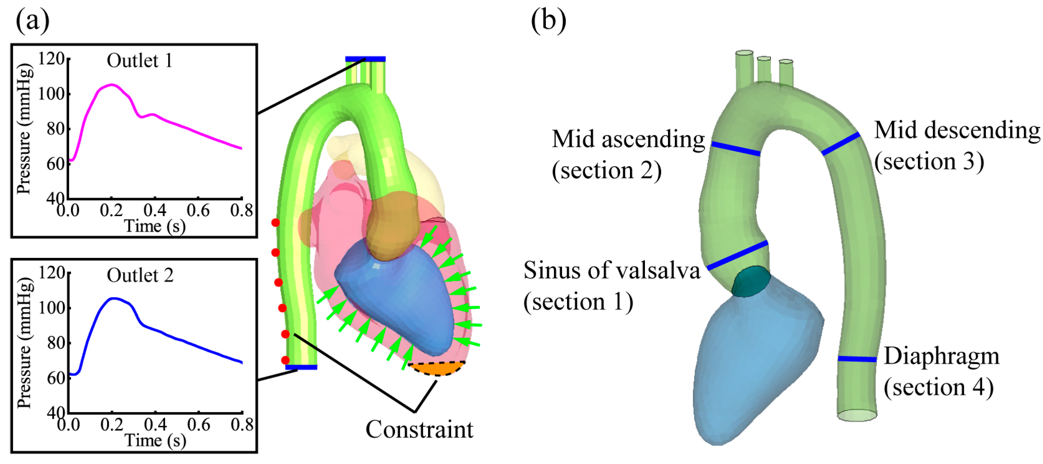
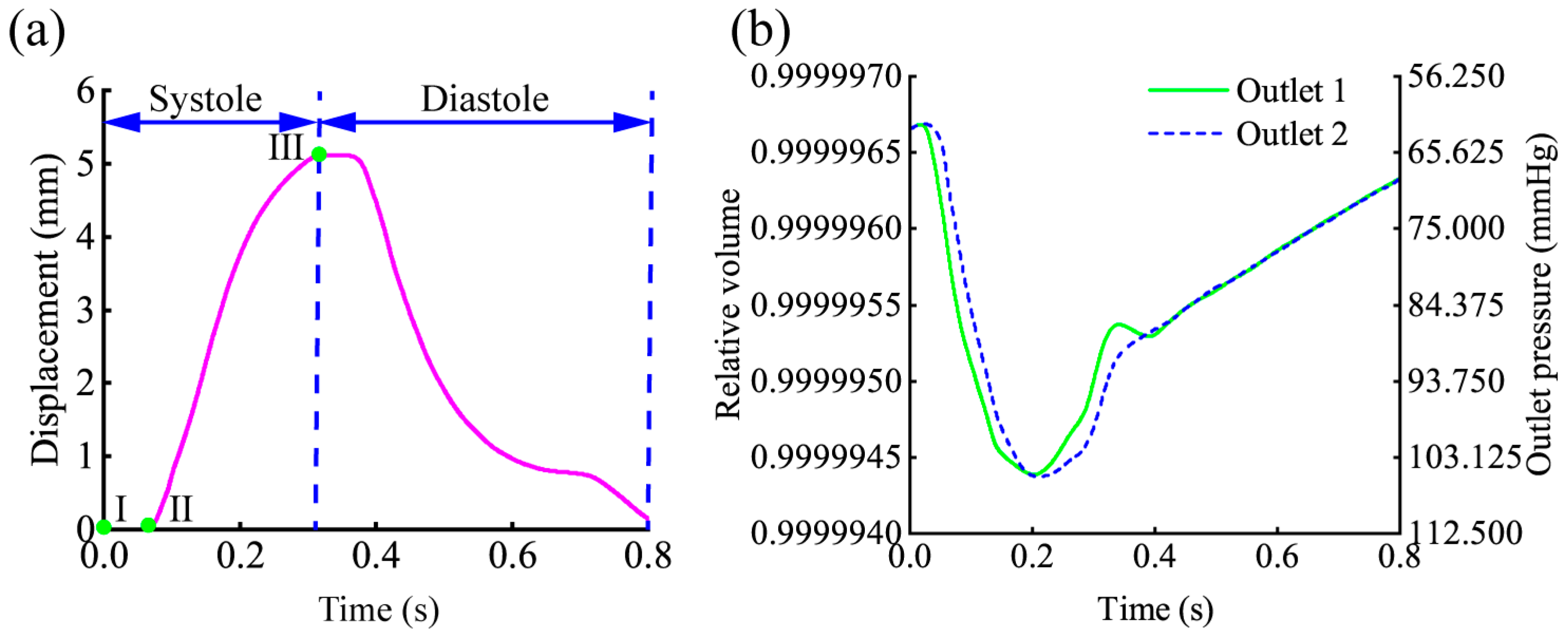
2.3. Simulation Boundary and Output Settings

The normal physiological boundaries and constraints of the heart–aorta FSI model are shown in Figure 4a. Reasonably constrained boundary conditions were set to the FSI model based on anatomical structural features. A full constraint was applied at the base of the heart (orange area in the dashed line) to simulate a fixed connection between the heart and the diaphragm. Radial constraints were set in part of the descending aorta (red dots) to achieve attachment between the intercostal arteries and the thoracic spine. Figure 4b shows the output locations of aortic hemodynamic parameters, analyzed for blood velocity, flow rate, and WSS at the aortic section.
Figure 5 represents the boundary load curves for the normal physiological state. The model simulated the systole and diastole of the heart by applying displacement loads to the LV (Figure 5a), thereby realizing the pumping function of the heart. The load was directed toward the interior of the LV and was oriented perpendicular to the element. The opening and closing of the aortic valve were achieved by controlling the coupling between the aortic valve and the blood. The point I on the curve indicated that the LV started to contract. At the point II, the LV began to eject. At this point, the FSI was turned off to simulate the open state of the aortic valve. The LV stopped ejection at the point III, and the FSI was turned on to simulate the closed state of the aortic valve. Flow resistance in blood vessel was simulated by applying a time-dependent pressure load at the aortic outlet [35]. As shown in Figure 5b, the pressure curves are converted into time-dependent relative volume curves and assigned to the EOS to realize the pressure change at the outlet. When the parameters in the Gruneisen EOS equation (Equation (9)) are set to specific values S 1 = 1 , S 2 = S 3 = 0 , γ 0 = 2 , E = 0 , it degenerates into a linear equation:
p = ρ 0 C 2 ζ
By combining Equations (10) and (11), the following can be obtained:
V = ρ 0 C 2 p + ρ 0 C 2
Parameter C can be calculated using the Newton–Laplace equation:
C = K ρ 0
where K is the blood bulk modulus and ρ 0 is the blood density. The speed of sound propagation in blood was calculated to be 1543 m/s.

2.4. Analysis of Heart–Aorta FSI at Different Physiological States

In actual physiological processes, blood viscosity changes in response to factors such as erythrocyte specific volume and plasma protein concentration (especially fibrin content). Meanwhile, blood viscosity is also a core parameter that determines the WSS in the aortic wall. In order to investigate the effect of changes in blood viscosity on the hemodynamic response of the aorta, heart–aorta FSI models were established with gradient variations ranging from 0.0015 Pa·s, 0.0035 Pa·s, 0.0055 Pa·s, 0.0075 Pa·s, and 0.0095 Pa·s.
LV ejection is the driving force of aortic blood flow. To investigate the effect of changes in LV ejection volume on the hemodynamic response of the aorta, changes in physiological state were achieved by scaling the time-displacement loads applied to the LV (Figure 5a). The ejection volume gradually increases as the LV motion displacement rising, as shown in Table 2. In our study, the normal physiologic state peak LV displacement was 5.1 mm with an ejection volume of 66.6 mL. The weakened systole pattern simulated the heart insufficiency with reduced ejection volume; the enhanced systole pattern simulated the exercise state with increased ejection volume.
The FSI model calculations were performed on a workstation equipped with an AMD EPYC 7T83 64-Core Processor (2.45 GHz). The LS-DYNA 971 R12.0 (LSTC, Livermore, CA, USA) version of the solver was used for the solution. The model required approximately 15 h of computation time during the cardiac cycle (0.8 s).

3. Results and Discussion

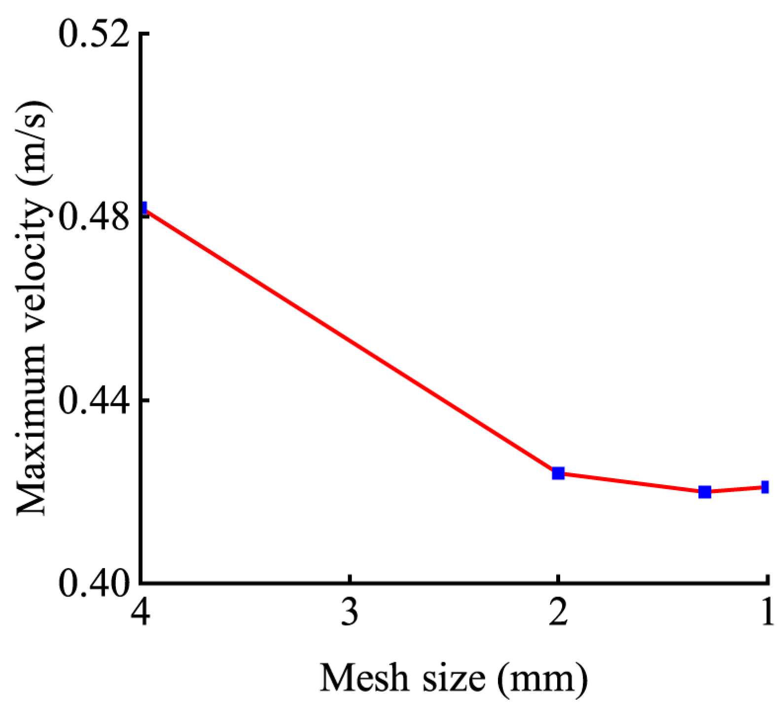
3.1. Mesh Sensitivity Analysis

Given the small diameter of the superior arteries, the baseline fluid domain mesh size was initially set to 4 mm. Structured meshes were constructed with 31, 30, and 48 defined points along the x, y, and z directions, respectively, controlled via the *ALE_STRUCTURED_MESH_CONTROL_POINT. The change in mesh size was achieved using the *ALE_STRUCTURED_MESH_REFINE keyword. Since the keyword parameter only supports integers, four different resolution computational fluid domains were established in the following sequence: 4 mm, 2 mm, 1.3 mm, and 1 mm. The results of the mesh sensitivity analysis of the section-averaged maximum blood velocity at the aortic root are shown in Figure 6.
When the mesh size was less than 2 mm, the maximum velocity demonstrated a gradual convergence trend. The mesh sensitivity analysis of the section-averaged maximum velocity was within 2% with a mesh size of 2 mm, indicating that the calculation convergence requirements had been met. The current structured fluid domain meshes were 357,120.

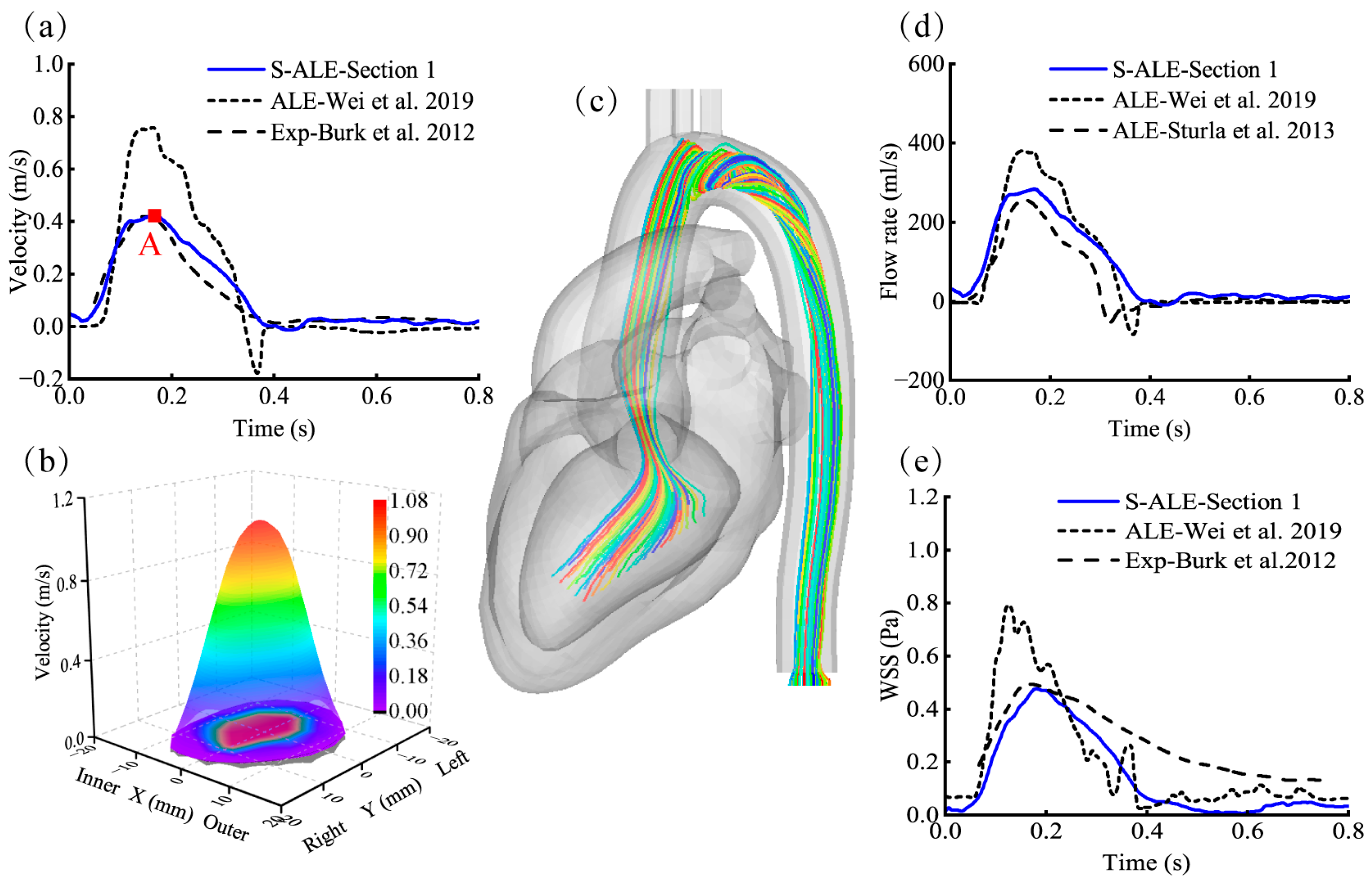
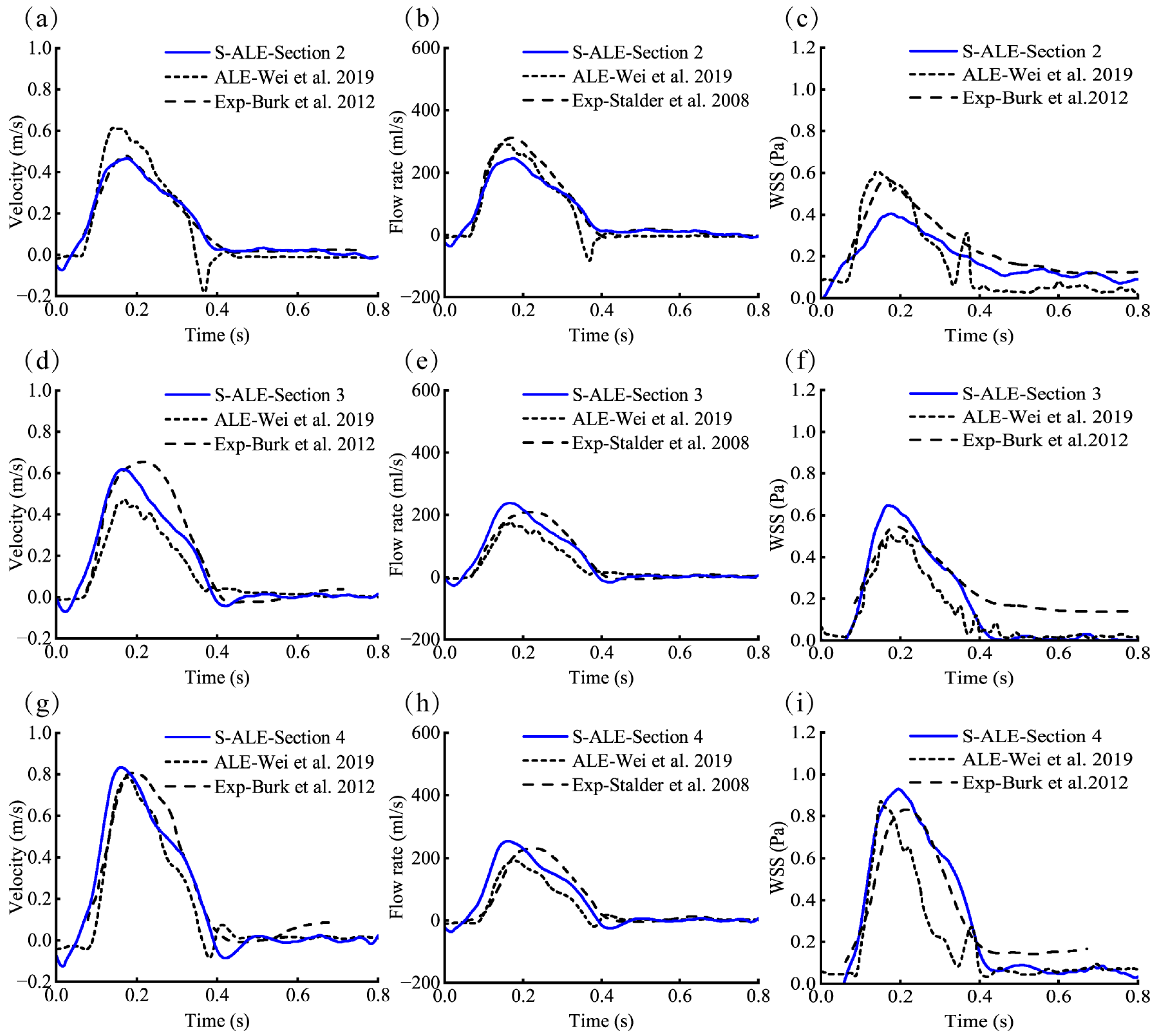
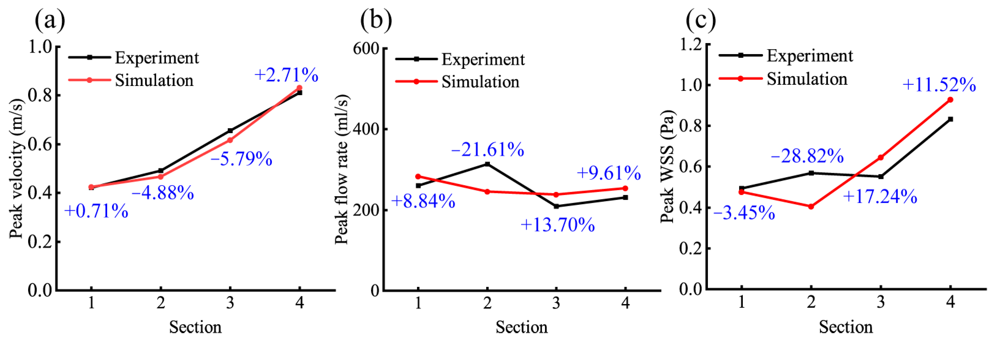
3.2. Validation of the FSI Numerical Model

The heart–aorta FSI model based on S-ALE method was validated for the hemodynamics of the aorta under a normal physiological state (blood viscosity 0.0035 Pa·s and peak LV displacement 5.1 mm) to ensure the simulation’s reliability. Hemodynamic parameters (blood velocity, flow rate, and WSS) for aortic sections 1–4 were validated against the published ALE method [23,24] and data measured by CMR experiments [3,4] in the literature.
Figure 7 demonstrates the blood flow and WSS at section 1. The average blood velocity time history curve is shown in Figure 7a, which is obtained by calculating the arithmetic mean of all nodal velocities in the section. Figure 7b shows the velocity distribution at the point A (0.168 s). From the streamline diagram (Figure 7c), it can be observed that there is turbulence in the blood at the aortic arch. Numerical simulation results indicated that the peak blood velocity was 0.42 m/s at section 1, while the peak velocities at the other sections, 2–4, ranged from 0.46 to 0.83 m/s. Figure 7d displays the flow rate variation curve, which is calculated by multiplying the section-averaged velocity with the real-time area variation. The peak flow rate at section 1 was 283.4 mL/s and the other sections, 2–4, were 238.1–253.7 mL/s.
Figure 7e demonstrates the section-averaged WSS of the aorta. The calculation of WSS is based on the local blood velocity gradient and blood viscosity, which are solved by the gradient tensor method. W S S = μ ( d ν / d x ) , where μ is the blood viscosity, ν is blood velocity along the direction of vessel, and x is the distance from the wall along its inward normal direction. The results showed that the peak WSS at section 1 was 0.47 Pa and the other sections, 2–4, were 0.40–0.93 Pa. The hemodynamic parameters of sections 2–4 are shown in Figure 8.
The comparison of peak hemodynamic parameters between numerical simulation and experimental data is shown in Figure 9. The analysis results indicated that the peak blood velocities obtained from the simulation were highly consistent with the experiment measurements, with a maximum relative error of less than 6%. In terms of section parameter comparison, except for the peak flow rate and WSS of section 2, which deviated from the experimental data by slightly more than 20%, the differences between the parameters of all other sections and the experimental results were within 20%.
The S-ALE method used in this study had good consistency with the data measured by CMR experiments. However, the hemodynamic parameters of section 1 were significantly different from the results obtained by the ALE method used by Wei et al. [23]. The blood velocity and WSS simulated by the ALE method were almost twice that of the S-ALE method, and the reason for this phenomenon was the difference in aortic root diameter (Table 1). In their study, the finite element model of the aorta was obtained by scaling, and its diameter had a larger difference compared to the actual anatomical structure. The analysis of the simulation results shows that the heart–aorta FSI model developed based on the S-ALE method has good reliability and can provide support for subsequent studies.

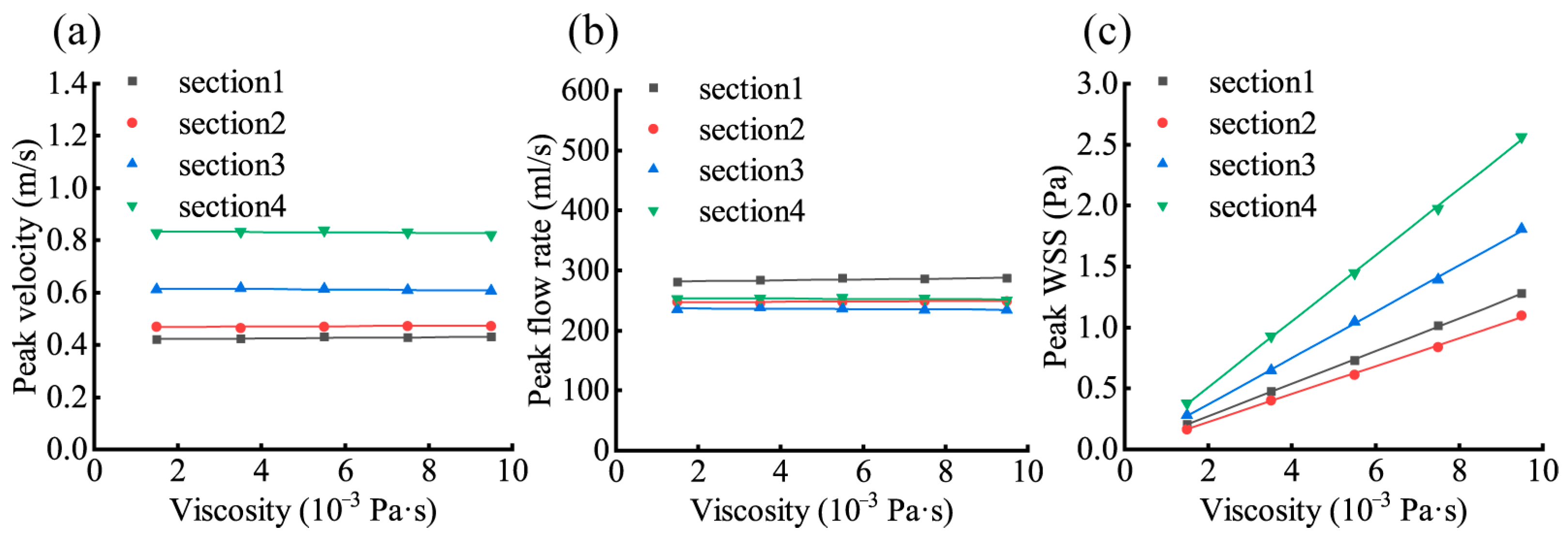
3.3. Effect of Changes in Blood Viscosity on the Aortic Hemodynamic Response

This study used viscosity coefficient as the input variable, with peak blood velocity, flow rate, and WSS as output variables. Through numerical simulations of five independent samples, quantitative response relationships between these hemodynamic parameters were established. Figure 10 shows the effect of changes in blood viscosity on aortic hemodynamic responses. From the figure, it can be observed that there is an approximately linear relationship between the viscosity coefficient and hemodynamic parameters. The Pearson correlation coefficient r was adopted to quantify the correlation between output and input variables, with an absolute value of r closer to 1 indicating stronger linear correlation and closer to 0 indicating weaker linear correlation. The mathematical expression is as follows:
r = i = 1 n x i x ¯ y i y ¯ i = 1 n x i x ¯ 2 i = 1 n y i y ¯ 2
where n is the sample size, x i is the viscosity coefficient value of the i-th sample, x ¯ is the sample mean of the viscosity coefficient, y i is the observed value of the i-th sample, and y ¯ represents the mean of the observed sample values. The correlation coefficients between the outputs and inputs in sections 1–4 are summarized in Table 3. The results showed that the peak WSS exhibited the strongest correlation, with its coefficient value approaching nearly 1. In contrast, weaker correlations were observed for both peak velocity and peak flow rate.
To further analyze the sensitivity of the viscosity coefficient to hemodynamic parameters, the slope of the linear regression model was adopted as a quantitative sensitivity indicator. Linear fitting was performed for the five sample groups, with the mathematical expression given by the following:
y = m x + b
where m is the slope and b is the intercept. The optimal slope m and intercept b were determined through least squares fitting by minimizing the residual sum of squares:
m = n i = 1 n x i y i i = 1 n x i i = 1 n y i n i = 1 n x i 2 i = 1 n x i 2 b = i = 1 n y i m i = 1 n x i n
Due to the dimensional differences among blood velocity, flow rate, and WSS, the fitted slope m was normalized through dimensionless processing, calculated as follows:
ε = m y ¯
The sensitivity analysis revealed that under different viscosity coefficients, the fitted slopes for both peak velocity and flow rate approached 0, with the fitted curves approximating straight lines parallel to the x-axis. This indicated that changes in the viscosity coefficient had no significant effect on peak velocity and flow rate in sections 1–4. In contrast, the WSS showed a clear increasing trend.
In our study, WSS was calculated by multiplying the viscosity coefficient with the velocity gradient of the section. The blood velocity tends to stabilize in sections 1–4, as shown in Figure 10a, which implies that the viscosity coefficient has no effect on the change in the velocity gradient. Therefore, the velocity gradient could be regarded as a constant. WSS was only related to the viscosity coefficient and exhibited a linear relationship. The peak WSS shown in Figure 10c confirms this conclusion. Fadhil et al. [19] similarly analyzed blood viscosity factors. In their study, an increase in the blood viscosity coefficient led to a decrease in blood velocity. We believe that the primary reason for this phenomenon is that the resistance to blood flow at the outlet of the aorta had not been taken into account in their simulations, which did not correspond to the blood flow in real situations. Also, WSS was not considered in their study.
Figure 10b presents the peak flow rate observed in sections 1–4 under different blood viscosity coefficients. The magnitude of flow rate was determined by the velocity and sectional area. However, there was no significant difference in the blood velocity through the sections for various viscosity coefficients, indicating that the sectional area did not change during blood flow. Therefore, it could be inferred that changes in blood viscosity had no effect on aortic deformation.

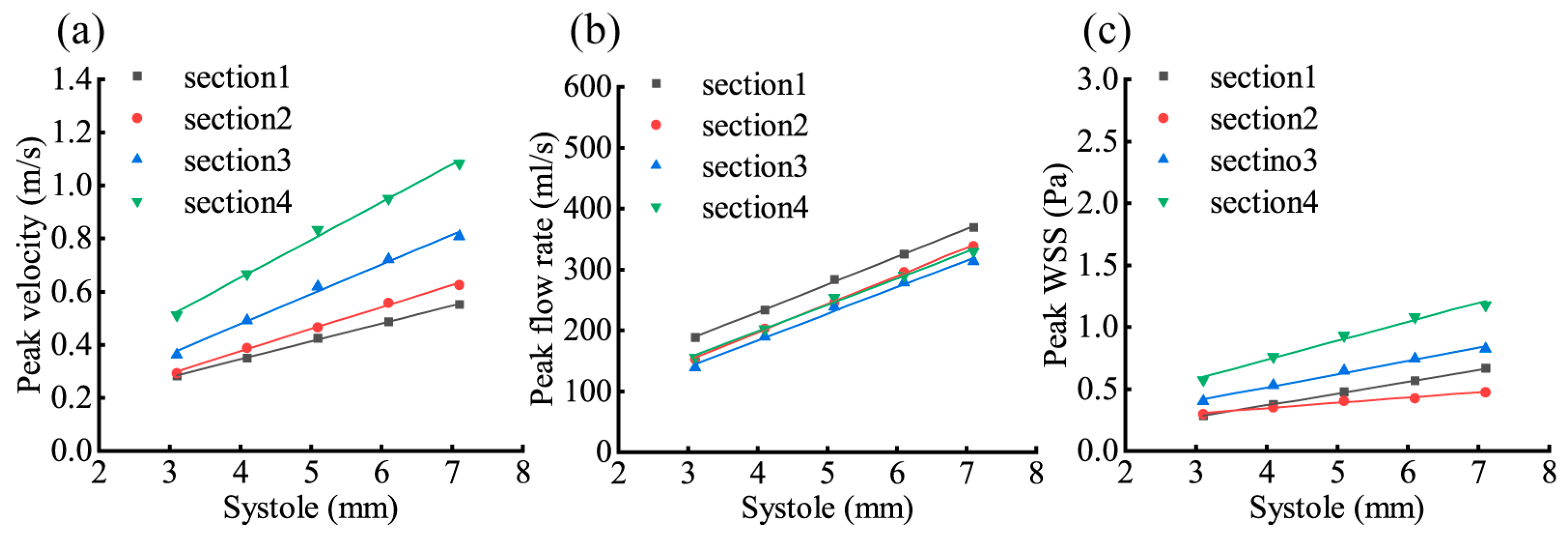
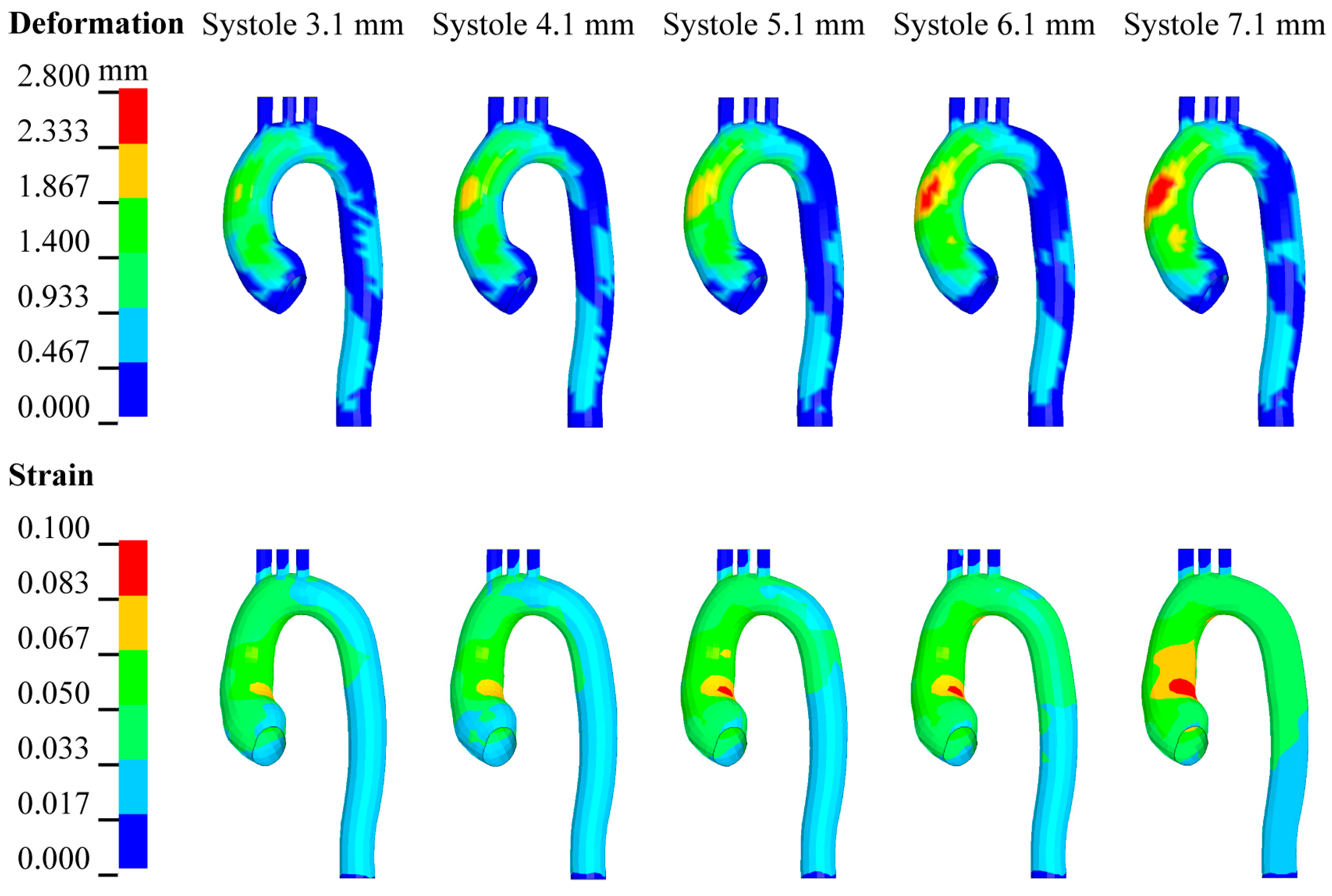
3.4. Effect of Changes in LV Systole on Aortic Hemodynamic Response

The ejection function of the heart changes in different physiological states, and the fundamental reason for this phenomenon is the change in the systole displacement of the LV. The effect of changes in LV systole on the aortic hemodynamic response at a blood viscosity of 0.0035 Pa·s is shown in Figure 11. From the figure, it can be observed that with the increase in LV systole displacement, the peak blood velocity, flow rate, and WSS of sections 1–4 showed an increasing trend. The quantitative analysis of the effect of systole displacement on aortic hemodynamic parameters is shown in Table 4. The analysis reveals that the correlation coefficients between systole displacement and hemodynamic parameters are close to 1, demonstrating significant linear correlations. The sensitivity analysis indicates that systole displacement exerts a substantial influence on hemodynamic parameters.
In our study, the resistance to blood flow at the aortic outlet did not change. The increased systole displacement of the LV resulted in an increase in the volume of blood ejected (Table 2), which was the reason for the increase in blood velocity. Aortic deformation tended to increase significantly with increasing LV systole displacement, as shown in Figure 12. The maximum deformation of the aorta was located in the region of the ascending aorta. The increase in aortic deformation indicated that the sectional area would also change. The maximum strain of the aorta occurred at the inner side of the root. The area of strain gradually expanded with the increasing systole displacement of the LV.
For the analysis of heart–aorta FSI, the LS-DYNA v971 R12.0 software is able to realize large deformation motions in the structural domains. This is a key factor in reproducing the hemodynamics of the systole and diastole processes in the LV. Most of the existing studies on aortic FSI have imposed time-dependent blood velocities at the root inlet location. Although it is possible to quantitatively study hemodynamic parameters, there is still a big gap with real human blood flow. There are also some limitations in our study. In the analysis of changes in different physiological states, variations in blood viscosity and LV ejection volume were assumed to occur without changes in rheological behavior, where blood was still treated as a Newtonian fluid. During the diastole phase, the absence of blood replenishment in the LV limited the heart–aortic FSI simulation to a single cardiac cycle under physiological states.

4. Conclusions

In this paper, a heart–aorta FSI model was developed by using the S-ALE method. The model implemented a coupled analysis of aorta and blood under physiological states by simulating LV systole motion. This work applied the S-ALE method to an FE model of the complex heart–aorta system. The simulation reliability of the model was effectively verified by comparing the ALE method and CMR experimental data. The aortic hemodynamic response under different physiologic states suggested that changes in blood viscosity only affected the WSS, whereas the key factor that really dominated the hemodynamic changes was the altered systole pattern of the LV. The model can be further integrated into a human biomechanical model to consider the injury mechanisms of hemodynamics on the aorta during large deformation collisions.

Author Contributions

Conceptualization, X.L. and J.C.; methodology, F.L.; software, X.L.; validation, X.L.; formal analysis, X.L. and X.C.; investigation, F.L.; resources, J.C.; data curation, X.L. and X.C.; writing—original draft preparation, X.L.; writing—review and editing, X.L. and J.C.; visualization, F.L.; supervision, F.L.; project administration, X.C.; funding acquisition, J.C. All authors have read and agreed to the published version of the manuscript.

Funding

This work is supported by the National Natural Science Foundation of China under Grant No. 52175267 and No. 52475297 and the National Automobile Accident In-Depth Investigation System (NAIS) Funding Project of China.

Institutional Review Board Statement

Not applicable.

Informed Consent Statement

Not applicable.

Data Availability Statement

The data presented in this study are available on request from the corresponding author. The data are not publicly available due to privacy.

Conflicts of Interest

The authors declare no conflicts of interest.

References

  1. Wang, X.; Ghayesh, M.H.; Kotousov, A.; Zander, A.C.; Dawson, J.A.; Psaltis, P.J. Fluid-structure interaction study for biomechanics and risk factors in Stanford type A aortic dissection. Int. J. Numer. Meth. Biomed. Eng. 2023, 39, e3736. [Google Scholar] [CrossRef] [PubMed]
  2. Mesri, A.; Niazmand, H.; Deyranlou, A.; Reza, S.M. Fluid-structure interaction in abdominal aortic aneurysms: Structural and geometrical considerations. Int. J. Mod. Phys. C 2015, 26, 1550038. [Google Scholar] [CrossRef]
  3. Burk, J.; Blanke, P.; Stankovic, Z.; Barker, A.; Russe, M.; Geiger, J.; Frydrychowicz, A.; Langer, M.; Markl, M. Evaluation of 3D blood flow patterns and wall shear stress in the normal and dilated thoracic aorta using flow-sensitive 4D CMR. J. Cardiovasc. Magn. Reson. 2012, 14, 84. [Google Scholar] [CrossRef]
  4. Stalder, A.F.; Russe, M.F.; Frydrychowicz, A.; Bock, J.; Hennig, J.; Markl, M. Quantitative 2D and 3D phase contrast MRI: Optimized analysis of blood flow and vessel wall parameters. Magn. Reson. Med. 2008, 60, 1218–1231. [Google Scholar] [CrossRef]
  5. Hirschhorn, M.; Tchantchaleishvili, V.; Stevens, R.; Rossano, J.; Throckmorton, A. Fluid-structure interaction modeling in cardiovascular medicine-A systematic review 2017–2019. Med. Eng. Phys. 2020, 78, 1–13. [Google Scholar] [CrossRef] [PubMed]
  6. Syed, F.; Khan, S.; Toma, M. Modeling dynamics of the cardiovascular system using fluid-structure interaction methods. Biology 2023, 12, 1026. [Google Scholar] [CrossRef]
  7. Hou, T.; Wei, X.; Iqbal, A.A.; Yang, X.; Wang, J.; Ren, Y.; Yan, S. Advances in biomedical fluid–structure interaction: Methodologies and applications from an interfacing perspective. Phys. Fluids 2024, 36, 21301. [Google Scholar] [CrossRef]
  8. Mourato, A.; Valente, R.; Xavier, J.; Brito, M.; Avril, S.; de Sá, J.C.; Tomás, A.; Fragata, J. Computational modelling and simulation of fluid structure interaction in aortic aneurysms: A systematic review and discussion of the clinical potential. Appl. Sci. 2022, 12, 8049. [Google Scholar] [CrossRef]
  9. Abbas, S.S.; Nasif, M.S.; Al-Waked, R. State-of-the-art numerical fluid–structure interaction methods for aortic and mitral heart valves simulations: A review. Simul.-Trans. Soc. Mod. Sim. 2022, 98, 3–34. [Google Scholar] [CrossRef]
  10. Wu, Q.; He, Y.; Yu, Z.; Wang, J.; Fan, W. Fluid-structure interaction analysis of vessel-bridge-steel floating fender collisions. Ocean Eng. 2024, 295, 116828. [Google Scholar] [CrossRef]
  11. Shi, Y.; Yang, D.; Wu, W. Numerical analysis method of ship-ice collision-induced vibration of the polar transport vessel based on the full coupling of ship-ice-water-air. J. Ocean Eng. Sci. 2023, 8, 323–335. [Google Scholar] [CrossRef]
  12. Lopes, D.; Agujetas, R.; Puga, H.; Teixeira, J.; Lima, R.; Alejo, J.P.; Ferrera, C. Analysis of finite element and finite volume methods for fluid-structure interaction simulation of blood flow in a real stenosed artery. Int. J. Mech. Sci. 2021, 207, 106650. [Google Scholar] [CrossRef]
  13. Ong, C.W.; Kabinejadian, F.; Xiong, F.; Wong, Y.R.; Toma, M.; Nguyen, Y.N.; Chua, K.J.; Cui, F.S.; Ho, P.; Leo, H. Pulsatile flow investigation in development of thoracic aortic aneurysm: An in-vitro validated fluid structure interaction analysis. J. Appl. Fluid Mech. 2019, 12, 1855–1872. [Google Scholar] [CrossRef]
  14. Kemp, I.; Dellimore, K.; Rodriguez, R.; Scheffer, C.; Blaine, D.; Weich, H.; Doubell, A. Experimental validation of the fluid–structure interaction simulation of a bioprosthetic aortic heart valve. Australas. Phys. Eng. S. 2013, 36, 363–373. [Google Scholar] [CrossRef]
  15. Scotti, C.M.; Finol, E.A. Compliant biomechanics of abdominal aortic aneurysms: A fluid-structure interaction study. Comput. Struct. 2007, 85, 1097–1113. [Google Scholar] [CrossRef]
  16. Valente, R.; Mourato, A.; Brito, M.; Xavier, J.; Tomás, A.; Avril, S. Fluid-structure interaction modeling of ascending thoracic aortic aneurysms in SimVascular. Biomechanics 2022, 2, 189–204. [Google Scholar] [CrossRef]
  17. Hsu, M.; Bazilevs, Y. Blood vessel tissue prestress modeling for vascular fluid-structure interaction simulation. Finite Elem. Anal. Des. 2011, 47, 593–599. [Google Scholar] [CrossRef]
  18. Wang, X.; Li, X. Fluid-structure interaction based study on the physiological factors affecting the behaviors of stented and non-stented thoracic aortic aneurysms. J. Biomech. 2011, 44, 2177–2184. [Google Scholar] [CrossRef]
  19. Fadhil, N.A.; Hammoodi, K.A.; Jassim, L.; Al-Asadi, H.A.; Habeeb, L.J. Multiphysics analysis for fluid–structure interaction of blood biological flow inside three-dimensional artery. Curved Layer. Struct. 2023, 10, 20220187. [Google Scholar] [CrossRef]
  20. Issakhov, A.; Sabyrkulova, A.; Abylkassymova, A. Numerical modeling of the fluid-structure interaction during blood flow in a flexible stenotic aorta. Int. Commun. Heat Mass 2024, 158, 107857. [Google Scholar] [CrossRef]
  21. Taheri, R.A.; Razaghi, R.; Bahramifar, A.; Morshedi, M.; Mafi, M.; Karimi, A. Interaction of the blood components with ascending thoracic aortic aneurysm wall: Biomechanical and fluid analyses. Life 2022, 12, 1296. [Google Scholar] [CrossRef] [PubMed]
  22. Tango, A.M.; Salmonsmith, J.; Ducci, A.; Burriesci, G. Validation and extension of a fluid-structure interaction model of the healthy aortic valve. Cardiovasc. Eng. Technol. 2018, 9, 739–751. [Google Scholar] [CrossRef] [PubMed]
  23. Wei, W.; Kahn, C.J.F.; Behr, M. Fluid-structure interaction simulation of aortic blood flow by ventricular beating: A preliminary model for blunt aortic injuries in vehicle crashes. Int. J. Crashworthiness 2019, 3, 229–306. [Google Scholar] [CrossRef]
  24. Sturla, F.; Votta, E.; Stevanella, M.; Conti, C.A.; Redaelli, A. Impact of modeling fluid-structure interaction in the computational analysis of aortic root biomechanics. Med. Eng. Phys. 2013, 35, 1721–1730. [Google Scholar] [CrossRef]
  25. Lee, S.H.; Kent, R. Blood flow and fluid-structure interactions in the human aorta during traumatic rupture conditions. Stapp Car Crash J. 2007, 51, 211–233. [Google Scholar]
  26. Tong, F.; Lan, F.; Chen, J.; Li, D.; Li, X. Numerical study on the injury mechanism of blunt aortic rupture of the occupant in frontal and side-impact. Int. J. Crashworthiness 2023, 28, 270–279. [Google Scholar] [CrossRef]
  27. Maceira, A.M.; Prasad, S.K.; Khan, M.; Pennell, D.J. Normalized left ventricular systolic and diastolic function by steady state free precession cardiovascular magnetic resonance. J. Cardiovasc. Magn. Reson. 2006, 8, 417–426. [Google Scholar] [CrossRef]
  28. Crosetto, P.; Reymond, P.; Deparis, S.; Kontaxakis, D.; Stergiopulos, N.; Quarteroni, A. Fluid-structure interaction simulation of aortic blood flow. Comput. Fluids 2011, 43, 46–57. [Google Scholar] [CrossRef]
  29. Brown, S.; Wang, J.; Ho, H.; Tullis, S. Numeric simulation of fluid-structure interaction in the aortic arch. In Book Computational Biomechanics for Medicine; Wittek, A., Miller, K., Nielsen, P.M., Eds.; Springer: New York, NY, USA, 2013; pp. 13–23. [Google Scholar]
  30. Ruan, J.; El-Jawahri, R.; Chai, L.; Barbat, S.; Prasad, P. Prediction and analysis of human thoracic impact responses and injuries in cadaver impacts using a full human body finite element model. Stapp Car Crash J. 2003, 47, 299–321. [Google Scholar]
  31. Nevsky, G.; Jacobs, J.E.; Lim, R.P.; Donnino, R.; Babb, J.S.; Srichai, M.B. Sex-specific normalized reference values of heart and great vessel dimensions in cardiac CT angiography. AJR Am. J. Roentgenol. 2011, 196, 788–794. [Google Scholar] [CrossRef]
  32. Katritsis, D.; Kaiktsis, L.; Chaniotis, A.; Pantos, J.; Efstathopoulos, E.P.; Marmarelis, V. Wall shear stress: Theoretical considerations and methods of measurement. Prog. Cardiovasc. Dis. 2007, 49, 307–329. [Google Scholar] [CrossRef] [PubMed]
  33. Gao, F.; Guo, Z.; Sakamoto, M.; Matsuzawa, T. Fluid-structure interaction within a layered aortic arch model. J. Biol. Phys. 2006, 32, 435–454. [Google Scholar] [CrossRef] [PubMed]
  34. LSTC. LS-DYNA Keyword User’s Manual; Livermore Software Technology Corporation (LSTC): Livermore, CA, USA, 2021. [Google Scholar]
  35. Kim, H.J.; Vignon-Clementel, I.E.; Figueroa, C.A.; Ladisa, J.F.; Jansen, K.E.; Feinstein, J.A.; Taylor, C.A. On coupling a lumped parameter heart model and a three-dimensional finite element aorta model. Ann. Biomed. Eng. 2009, 37, 2153–2169. [Google Scholar] [CrossRef] [PubMed]
Figure 1. Schematic diagram of fluid–structure interaction principle.
Applsci 15 07769 g001
Figure 2. Establishment of FE model for structural domain. (a) Reverse modeling of FE model of aorta; (b) FE model of the heart–aorta system.
Applsci 15 07769 g002
Figure 3. Establishment of FE model for fluid domain. (a) Structured orthogonal three-dimensional mesh; (b) the generated blood model.
Applsci 15 07769 g003
Figure 4. Simulation boundaries and output settings for the heart–aorta FSI model. (a) Normal physiological boundary and constraint; (b) output locations of the aortic section.
Applsci 15 07769 g004
Figure 5. Boundary load curves at normal physiologic state. (a) LV motion displacement curve; (b) relative volume curve obtained from outlet pressure conversion.
Applsci 15 07769 g005
Figure 6. Fluid domain mesh sensitivity analysis.
Applsci 15 07769 g006
Figure 7. Blood flow and WSS at section 1 [3,23,24]. (a) Section-averaged blood velocity; (b) blood velocity distribution at the moment of point A; (c) partial blood flow stream line in the LV and aorta; (d) section-averaged blood flow rate; (e) section-averaged WSS.
Applsci 15 07769 g007
Figure 8. Blood flow and WSS at sections 2–4 [3,4,23]. (a,d,g) Section-averaged blood velocity; (b,e,h) section-averaged blood flow rate; (c,f,i) section-averaged WSS.
Applsci 15 07769 g008
Figure 9. Comparison of hemodynamic parameter errors between numerical simulation and experiment data. (a) Section-averaged peak velocity; (b) section-averaged peak flow rate; (c) section-averaged peak WSS.
Applsci 15 07769 g009
Figure 10. Effect of various in blood viscosity on aortic hemodynamic response. (a) Section-averaged peak velocity; (b) section-averaged peak flow rate; (c) section-averaged peak WSS.
Applsci 15 07769 g010
Figure 11. Effect of changes in LV systole on aortic hemodynamic response. (a) Section-averaged peak velocity; (b) section-averaged peak flow rate; (c) section-averaged peak WSS.
Applsci 15 07769 g011
Figure 12. Aortic deformation and strain distribution response under changes in LV systole.
Applsci 15 07769 g012
Table 2. LV systole patterns in different physiological states.
Weakened SystoleNormal SystoleEnhanced Systole
LV systole schematic
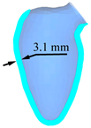
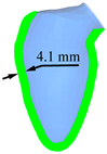
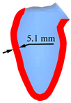
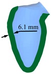
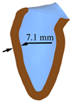
Applsci 15 07769 i001Applsci 15 07769 i002Applsci 15 07769 i003Applsci 15 07769 i004Applsci 15 07769 i005
Peak displacement3.1 mm4.1 mm5.1 mm6.1 mm7.1 mm
Ejection volume49.4 ml58.3 ml66.6 ml74.2 ml81.2 ml
Table 3. Quantitative analysis of the effects of viscosity coefficient on aortic hemodynamic parameters.
SectionPeak VelocityPeak Flow RatePeak WSS
rεrεrε
10.87460.00250.88100.00250.99990.1814
20.65100.00130.68520.00130.99960.1840
3−0.6318−0.0015−0.6581−0.00130.99970.1836
4−0.6260−0.0010−0.6020−0.00100.99970.1858
Table 4. Quantitative analysis of the effects of systole displacement on aortic hemodynamic parameters.
SectionPeak VelocityPeak Flow RatePeak WSS
rεrεrε
10.99960.16200.99960.16220.99980.2028
20.99980.17860.99960.18690.99350.1090
30.99680.18690.99710.18910.99570.1701
40.99780.17670.99780.17700.99320.1695
Disclaimer/Publisher’s Note: The statements, opinions and data contained in all publications are solely those of the individual author(s) and contributor(s) and not of MDPI and/or the editor(s). MDPI and/or the editor(s) disclaim responsibility for any injury to people or property resulting from any ideas, methods, instructions or products referred to in the content.

