Service Composition and Optimal Selection for Industrial Software Integration with QoS and Availability

Abstract

To address the growing demand for industrial software in the digital transformation of small and medium-sized enterprises (SMEs) in the manufacturing sector, and to ensure the stable integration and operation of multi-source heterogeneous industrial software under complex conditions—such as heterogeneous compatibility, component dependencies, and uncertainty disturbances—this study established a comprehensive evaluation index system for service composition and optimal selection (SCOS). The system incorporated key criteria including service time, service cost, service reputation, service delivery quality, and availability. Based on this, a bi-objective SCOS model was established with the goal of maximizing both quality of service (QoS) and availability. To efficiently solve the proposed model, a hybrid enhanced multi-objective Gray Wolf Optimizer (HEMOGWO) was developed. This algorithm integrated Tent chaotic mapping and a Levy flight-enhanced differential evolution (DE) strategy. Extensive experiments were conducted, including performance evaluation on 17 benchmark functions and case studies involving nine industrial software integration scenarios of varying scales. Comparative results against state-of-the-art, multi-objective, optimization algorithms—such as MOGWO, MOEA/D_DE, MOPSO, and NSGA-III—demonstrate the effectiveness and feasibility of the proposed approach.

1. Introduction

As the manufacturing industry accelerates its transition toward digitalization and intelligentization, industrial software has become a vital tool for SMEs to improve operational efficiency and reduce management costs. By integrating business processes and optimizing production and management activities, industrial software effectively eliminates information silos, thereby enabling data sharing and facilitating cross-functional business collaboration [1]. Nevertheless, SMEs commonly face practical challenges such as limited financial resources and inadequate technical support. Addressing diverse business requirements within such constraints has become a pressing issue. Especially during the software selection and system integration process, compatibility differences between software from different vendors and of different types often lead to duplicated investments and increased maintenance costs, further exacerbating resource pressure. To tackle this problem, industrial software platforms based on standardized data interfaces have been developed to resolve compatibility issues among heterogeneous software systems originating from different vendors and application domains, thereby establishing a technical foundation for SCOS. These platforms analyze user requirements and intelligently identify software combinations that are functionally compatible, cost-efficient, and capable of strong collaboration. This supports systematic optimization across key business areas, including production, management, and service delivery.

However, under the context of the deep integration of multi-source heterogeneous systems, the stable operation of industrial software service composition schemes heavily depends on the effective coordination and integration of these heterogeneous components. In complex multi-system integration scenarios, insufficient adaptability to heterogeneous environments may lead to latent errors such as data parsing failures. Cross-component dependencies can trigger cascading faults, while sudden traffic surges may result in resource contention [2]. These non-deterministic failures often manifest as response delays and data processing anomalies, which degrade the overall functionality of the integrated system. In severe cases, such issues can cause system-wide crashes, forcing enterprises to halt shop-floor operations entirely and delay order delivery, thereby severely disrupting business continuity and adversely affecting economic performance. Therefore, ensuring the stability of industrial software service compositions under uncertainty is of critical importance.

Currently, to ensure the stable operation of SCOS, extensive research has focused on handling service anomalies and enhancing robustness in complex scenarios. Gao et al. [3] established a service composition adaptive adjustment framework composed of three parts: anomaly detection, anomaly diagnosis, and anomaly processing. Yang [4] improved the robustness of cloud manufacturing services by assigning both preferred and alternative services to each subtask. Zhao et al. [5], addressing the reconfiguration problem of cloud manufacturing service composition in failure handling, introduced an enhanced CMSCR method featuring flexible decomposition and a hybrid strategy. Yang et al. [6] proposed a strategy of proactive SC and the process of reactive service adjustment, which effectively reduced the reservation cost of robust service composition. Yin et al. [7] addressed the issue of QoS assurance following service anomalies in cloud service composition, proposing an adaptive anomaly adjustment method based on gray relational analysis to optimize service time, cost, reliability, quality, and compatibility. Gao et al. [8] constructed a robustness index that comprehensively considers the abnormal probability, delay time, and execution time of subtasks to quantify the service anti-interference ability under abnormal conditions. Zhang [9] introduced an adaptive robust SCOS model, which incorporates an alternative service invocation strategy. This model evaluates task delays based on whether to wait for service recovery or to invoke alternative services, thereby serving as a basis for robustness assessment. However, industrial software integration systems operate in environments that demand high real-time performance and reliability. In such contexts, traditional approaches—such as pre-configured alternative services or dynamic adjustment mechanisms—are often limited in practical applicability when dealing with service anomalies. Therefore, it is necessary to introduce evaluation metrics that more accurately reflect the system’s capability for sustained service delivery. Availability, as a key metric for assessing a system’s ability to continuously provide services [10], not only encompasses dimensions such as MTBF and failure recovery efficiency, but also integrates aspects of reliability, robustness, and other related quality attributes. Hence, availability should be considered as an independent performance evaluation criterion.

The MOGWO has been widely applied to multi-objective optimization problems in engineering due to its advantages such as fast convergence speed, a small number of parameters, and ease of adjustment. Ni et al. [11] integrated an improved MOGWO with the TOPSIS method to optimize process parameters in high-speed dry hobbing. Xue et al. [12] employed MOGWO to achieve adaptive denoising of acoustic signals from gas pipeline leaks under multiple operating conditions. Liu et al. [13] proposed a MOGWO algorithm combined with multiple search strategies for the multi-objective scheduling problem of cascade hydropower stations. Wynn et al. [14] combined NSGA-II with MOGWO, incorporating demand response and uncertainty modeling of renewable energy to achieve peak–valley load regulation in power systems. Dong et al. [15] proposed an IMOGWO incorporating a predatory behavior-inspired search strategy to address the collaborative optimization scheduling problem in green manufacturing within distributed heterogeneous semiconductor wafer fabrication facilities. Chen et al. [16] proposed a MOGWO method based on machine learning to realize the collaborative optimization of the safety of lightweight automobile seat frames. Nadimi-Shahraki et al. [17] proposed a hunting search strategy based on dimension learning to address global optimization and engineering design problems, aiming to alleviate issues such as lack of diversity and premature convergence. Despite the extensive research efforts devoted to the improvement and application of the MOGWO method, its convergence performance remains suboptimal, and it is prone to becoming trapped in local optima.

To address the resource composition optimization challenges in current industrial software integration, this study proposes a multi-objective optimization model that balances performance and reliability, guided by both QoS constraints and service availability requirements. To efficiently solve this model and improve solution quality, a HEMOGWO algorithm is introduced. The algorithm enhances the quality of the initial population using Tent chaotic mapping and improves global search capability and diversity by integrating a differential evolution strategy with Lévy flight, effectively avoiding local optima. Experimental validation is conducted on both standard benchmark functions and real-world industrial software composition scenarios, demonstrating that the proposed method offers significant advantages over existing approaches in terms of solution distribution, convergence speed, and stability.

2. Problem Statement

To effectively support the SCOS of industrial software resources, this chapter provides a detailed discussion of the core processes and relevant metrics of multi-objective optimization. It focuses on key factors such as QoS and availability and establishes the corresponding mathematical model to lay the foundation for subsequent SCOS implementation.

2.1. Process of SCOS

In industrial software platforms, each user-submitted requirement is treated as an independent task. Based on the user’s specific business scenario, the platform further decomposes the task into multiple software functional subtasks and performs resource search and matching within the service cloud pool to support subsequent SCOS. As illustrated in Figure 1, the SCOS process in industrial software can be divided into the following five key steps:

• User Requirement Submission: The user, based on their specific business scenario, provides a preliminary functional requirement or objective.
• Task Decomposition: The user requirements are modularly decomposed to extract core functional features, which are then further subdivided into multiple sub-tasks for detailed execution.
• Service Search and Matching: For each subtask, the system matches all suitable candidate software resources from the service cloud pool according to the user’s quality of service and functional requirements and generates the corresponding set of software resources.
• SCOS: The industrial software platform selects appropriate software from the resource set corresponding to each subtask and generates a Pareto-optimal set of service compositions that satisfy the constraints, based on a multi-objective optimization model.
• Task Feedback and Execution: All optimal composition solutions are returned to the user, who selects and executes the preferred one.

This study focuses on the fourth stage of the above process—service composition optimization. The optimization results at this stage have a direct impact on both the efficiency and effectiveness of the platform’s service delivery to users and therefore hold significant research value.

2.2. QoS Criterion of SCOS

QoS is a critical non-functional attribute for evaluating the capability of software services and is widely applied in SCOS to assess whether a service meets the user’s performance expectations. QoS not only enables users to select software according to their individual preferences but also provides a theoretical foundation for service evaluation. At present, a relatively systematic evaluation framework for QoS in SCOS has been established. In this study, four of the most commonly used QoS attributes are selected for modeling and optimization: Time (T), Cost (C), Reputation (Re), and Quality (Q) [18]. The aggregation of QoS attributes is influenced by the structure of the service composition. Common service structures include sequential, parallel, conditional, and loop structures, and existing research has extensively discussed the transformation methods among these structures [19]. To simplify the model and achieve accurate representation, this study focuses exclusively on sequential structures for modeling and QoS computation. The comprehensive evaluation function of QoS in SCOS is shown in Equation (1).

$$QoS(CMS)={\omega }_T\times Q_T+{\omega }_C\times Q_C+{\omega }_{Re}\times Q_{Re}+{\omega }_Q\times Q_Q$$

(1)

where ω_T, ω_C, ω_Re, ω_Q represent the weight coefficients of time, cost, reputation, and quality, respectively, ω ∈ [0, 1] and ω_T + ω_C + ω_Re + ω_Q = 1.

Table 1. The sequential type’s aggregate QoS attributes.

QoS Indicator	Function	Meaning	Attribute
T	$Q_T={\displaystyle {\sum }_{j=1}^n{q}_T(S{T}^j)/n}$	Includes deployment and debugging time for industrial software	Negative
C	$Q_C={\displaystyle {\sum }_{j=1}^n{q}_C(S{T}^j)/n}$	Costs of procurement, maintenance, hardware, implementation, and licensing of industrial software	Negative
Re	$Q_{Re}=\sqrt[n]{{\displaystyle \prod _{j=1}^n{q}_{Re}(S{T}^j)}}$	Reputation of candidate industrial software resources	Positive
Q	$Q_Q={\displaystyle {\sum }_{j=1}^n{q}_Q(S{T}^j)/n}$	Product quality	Positive

presents the aggregation functions for the four QoS attributes.

Due to the significant differences in dimensions, value ranges, and evaluation criteria among various QoS attributes, normalization of the original QoS data is required to facilitate unified modeling and comparison in subsequent stages. In this context, “Positive” refers to attributes where higher values indicate better performance, while “Negative” refers to attributes where lower values are preferred. Therefore, QoS attributes can be classified into beneficial and non-beneficial types [20]. These attributes are normalized using Equation (2).

$$q_k=\left\{\begin{array}{ll}{\displaystyle \frac{x_{\max }-x_k}{x_{\max }-x_{\min }}},\hfill & x_k is a negative attribute\hfill \\ {\displaystyle \frac{x_k-x_{\min }}{x_{\max }-x_{\min }}},\hfill & x_k is a positive attribute\hfill \end{array}\right.$$

(2)

where x_max and x_min denote the maximum and minimum values of the corresponding QoS attribute, respectively. In addition, when x_max = x_min, q_k = 1. After normalization, all QoS attribute values are scaled to the [0, 1] interval, which facilitates the trade-off and integration of multiple attributes within multi-objective optimization algorithms.

2.3. Availability Metrics of SCOS

In the era of Industry 4.0 and intelligent manufacturing, integrated systems of industrial software such as ERP, MES, and WMS are required to operate collaboratively on a 24/7 basis without interruption. The continuity and efficiency of these systems are directly linked to the economic performance of enterprises.

Table 2. The maximum allowable downtime of the system theory.

Availability	Downtime/90 Days	Downtime/1 Year
99%	21 h and 36 min	3 days 15.6 h
99.9%	2 h and 10 min	8 h and 45 min
99.99%	12 min and 58 s	52 min and 34 s
99.999%	1 min and 18 s	5 min and 15 s
99.9999%	8 s	32 s

presents the theoretical maximum allowable downtime over a 90-day and one-year period under different levels of availability. As a key functional metric for evaluating the sustainable operational capability of services, availability is defined as the ratio of the time a system remains in an operational state to the total operational period [21]. The modeling process for composite availability in multi-source heterogeneous industrial software integration is outlined as follows.

1.

Definition of the service component set: In the context of heterogeneous industrial software integration, assume there are n industrial software components originating from different vendors and built on different technology stacks. The expression is given in Equation (3).

$$S=\{s_1,s_2,\dots ,s_n\}$$

(3)

2.

Computation of individual component availability: for each component s_i, its availability A_i is calculated using Equation (4).

$$A_i={\displaystyle \frac{MTB{F}_i}{MTB{F}_i+MTT{R}_i}}$$

(4)

where MTBF represents the average time the system operates without failure, reflecting its inherent reliability, and MTTR denotes the average time required to diagnose, repair, and restore the system to operational status. For example, if the MTBF of an industrial software component is 200 h and the MTTR is 20 h, its availability A_i can be calculated as follows according to Equation (4):

$$A_i={\displaystyle \frac{MTB{F}_i}{MTB{F}_i+MTT{R}_i}}={\displaystyle \frac{200}{200+20}}=0.91$$

This value indicates that the component remains in a functional service state approximately 91% of the time during long-term operation.

3.

Construction of the dependency matrix: Based on the modeling of functional and logical dependencies, a dependency matrix D = [d_ij] is constructed to represent the strength of the dependency of component s_i on component s_j. The criteria for determining functional relationships are presented in

Table 3. Determination of functional relationships.

Functional Relationship	Dependency Strength
No direct dependency, logically unrelated	0
Control flow dependency (sequential)	0.5
Control flow dependency with enforced control	1

.

4.

Incorporation of integration uncertainty factors: Due to the unpredictability associated with the initial collaboration between services, additional integration risks often arise. Therefore, it is necessary to introduce an “integration uncertainty factor” in the modeling of composite availability to penalize the potential failure probability caused by first-time integration. A confidence factor θ_i is introduced to represent the reliability level of component s_i when integrated with other components. When a service has a history of successful integration, a high level of technological maturity, or a well-standardized interface, θ_i is set to 1, indicating high integration reliability. For newly introduced services, or in cases involving complex interfaces and significant vendor heterogeneity, θ_i is set to 0.5 to reflect the potential risk of uncertainty. In the model computation, the availability A_i of each service is multiplied by the corresponding θ_i, resulting in the adjusted service availability A_i·θ_i.

5.

Evaluation of overall system coupling: Components within a system often exhibit complex invocation and data dependency relationships. These dependencies determine the degree of system coupling and directly affect the overall stability and maintainability of the system. Therefore, it is essential to quantitatively assess system coupling within the availability modeling process, using it as a penalty factor for potential risks. A dependency matrix D = [d_ij] of size n × n is used to represent the dependency strength of component s_i on component s_j. Based on this matrix, the overall system coupling degree $\mathcal{C}$ can be calculated using Equation (5).

$$\mathcal{C}={\displaystyle \frac{1}{n(n-1)}}{\displaystyle \sum _{i\ne j}{d}_{ij}}$$

(5)

where n denotes the number of components.

6.

Composite availability modeling: to accurately reflect the operational reliability of the entire service portfolio, the availability model Equation (6) is established by comprehensively considering the factors mentioned above.

$$A_{combo}={\displaystyle \prod _{i=1}^n(\frac{MTB{F}_i}{MTB{F}_i+MTT{R}_i}\cdot {\theta }_i)}\cdot (1-\lambda \cdot \mathcal{C})$$

(6)

where λ ∈ [0.1, 0.3] represents the coupling penalty factor, θ_i denotes the confidence level of service integration, and $\mathcal{C}$ indicates the overall system coupling degree.

2.4. SCOS Mathematical Model

Based on the aforementioned availability modeling and QoS metric analysis, this study constructs a bi-objective SCOS model that simultaneously considers QoS and system availability. The model aims to satisfy both the functional and non-functional requirements of users while achieving optimal overall availability of the service composition. The objective function of the model can be formally expressed as Equation (7).

$$\left\{\begin{array}{l}Min f_1=1-QoS(CSS)\\ Min f_2=1-A(CSS)\\ F=[f_1,f_2]\end{array}\right.$$

(7)

where f₁ and f₂ represent the two optimization objectives of QoS and system availability, respectively, and CSS represents industrial software services on the platform.

3. Proposed HEMOGWO for SCOS

This section first introduces the original MOGWO and then proposes an enhanced method, HEMOGWO. Although MOGWO demonstrates strong search capabilities in solving multi-objective optimization problems, it still suffers from several limitations, including poor initial population quality, susceptibility to local optima, and insufficient solution diversity. These issues become more pronounced in practical applications such as industrial software resource composition, which often involve high-dimensional and highly constrained environments. To address these challenges, two key improvement strategies are proposed: (1) an initialization method based on Tent chaotic mapping is employed to enhance the uniformity of the initial population distribution, and (2) a hybrid mechanism combining Lévy flight and differential evolution is integrated to improve the algorithm’s global exploration and local exploitation capabilities during the later stages of the search, thereby enhancing population diversity and convergence speed.

3.1. Original MOGWO

The MOGWO was proposed by Mirjalili et al. [22] as a population-based metaheuristic optimization algorithm. It extends the classical GWO [23] and is specifically designed to solve multi-objective optimization problems. The algorithm is inspired by the hunting behavior and hierarchical structure of gray wolves in nature, which has led to its widespread application. The characteristics of MOGWO can be described from the following three aspects.

3.1.1. Social Hierarchy

The algorithm simulates the social hierarchy of gray wolves by dividing the pack into four levels: α, β, δ, and ω wolves. Among them, the α wolf represents the individual with the highest fitness, while the β and δ wolves have the second and third highest fitness values, respectively. These three top-performing wolves guide the rest of the pack, the ω wolves, in the processes of tracking, encircling, and attacking the prey.

3.1.2. Hunting Behavior

Gray wolves perform global searches to locate potential prey, a process that simulates the algorithm’s exploration of unknown areas within the solution space. The chasing behavior can be described by Equation (8).

$$\left\{\begin{array}{l}{\overrightarrow{D}}_{\alpha }=|{\overrightarrow{C}}_1\cdot {\overrightarrow{X}}_{\alpha }-\overrightarrow{X}|\hfill \\ {\overrightarrow{D}}_{\beta }=|{\overrightarrow{C}}_2\cdot {\overrightarrow{X}}_{\beta }-\overrightarrow{X}|\hfill \\ {\overrightarrow{D}}_{\delta }=|{\overrightarrow{C}}_3\cdot {\overrightarrow{X}}_{\delta }-\overrightarrow{X}|\hfill \end{array}\right.$$

(8)

where ${\overrightarrow{X}}_{\alpha }$, ${\overrightarrow{X}}_{\beta }$, ${\overrightarrow{X}}_{\delta }$ respectively represent the current optimal position of the α, β, δ, wolf; ${\overrightarrow{C}}_1$, ${\overrightarrow{C}}_2$, ${\overrightarrow{C}}_3$ denote random perturbation vectors, defined as ${\overrightarrow{C}}_1$ = 2⋅${\overrightarrow{r}}_1$, ${\overrightarrow{r}}_1$ ∈ [0, 1].

Subsequently, the wolves gradually reduce the encircling radius, which simulates the algorithm’s fine-grained search in local regions. Based on the positions of the α, β, and δ wolves, the other wolves update their movement direction according to Equation (9).

$$\left\{\begin{array}{l}{\overrightarrow{X}}_1={\overrightarrow{X}}_{\alpha }-{\overrightarrow{A}}_1\cdot {\overrightarrow{D}}_{\alpha }\hfill \\ {\overrightarrow{X}}_2={\overrightarrow{X}}_{\beta }-{\overrightarrow{A}}_2\cdot {\overrightarrow{D}}_{\beta }\hfill \\ {\overrightarrow{X}}_3={\overrightarrow{X}}_{\delta }-{\overrightarrow{A}}_3\cdot {\overrightarrow{D}}_{\delta }\hfill \end{array}\right.$$

(9)

where ${\overrightarrow{A}}_i$= 2⋅$\overrightarrow{a}$⋅${\overrightarrow{r}}_2$ − $\overrightarrow{a}$, $\overrightarrow{a}$ denotes the convergence factor, which decreases linearly from 2 to 0 with iteration; ${\overrightarrow{r}}_2$ is a random vector in [0, 1].

Finally, according to Equation (10), the position is updated as the average of the three.

$$\overrightarrow{X}(t+1)={\displaystyle \frac{{\overrightarrow{X}}_1+{\overrightarrow{X}}_2+{\overrightarrow{X}}_3}{3}}$$

(10)

When the prey ceases to move, the gray wolves initiate an attack, which corresponds to the local exploitation phase of the algorithm. The attacking behavior is controlled by the convergence factor $\overrightarrow{a}$, the value of which is calculated according to Equation (11) and decreases with the increase in the number of iterations.

$$\overrightarrow{a}=2-2{\displaystyle \frac{t}{T_{\max }}}$$

(11)

where t represents the current number of iterations, and T_max represents the maximum number of iterations. When the absolute value of $\overrightarrow{A}$ is $\left|\overrightarrow{A}\right|$ < 1, the algorithm enters the local development stage, and the gray wolf position is fine-tuned to approximate the exact solution.

3.1.3. Pareto Front Maintenance

The algorithm maintains the Pareto front by integrating an external archive with a leader selection strategy. The archive is used to store non-dominated solutions and is dynamically updated by comparing new candidate solutions with existing members. To manage the archive size, a grid mechanism is employed to divide the objective space into multiple hypercubes. When the archive reaches its capacity, the most crowded hypercube is identified, and one solution within it is randomly removed to accommodate the new solution, thereby ensuring a uniform distribution of the solution set. If a new solution falls outside the existing hypercubes, the grid is adaptively expanded. The selection of the α, β, and δ leaders is carried out using a roulette wheel method, in which candidates are chosen from the least crowded hypercubes. The selection probability is inversely proportional to the density of the hypercube.

3.2. Population Initialization

In the search mechanism of MOGWO, the distribution characteristics of the initial population directly influence the convergence speed and the quality of the optimization results. Traditional random initialization strategies employ a completely random distribution within the solution space. Although this approach is simple to implement, it may lead to uneven population distribution and low individual dispersion, making the search process prone to premature convergence and unstable efficiency. To address this issue, this study proposes a population initialization strategy based on Tent chaotic mapping. By leveraging the ergodicity and inherent regularity of chaotic systems, this method ensures population diversity while enabling uniform exploration of the solution space, thereby significantly enhancing the algorithm’s global search capability and convergence speed [24].

Tent chaotic mapping, as a typical one-dimensional chaotic system, exhibits dynamic behavior governed by a piecewise linear iterative equation. The mathematical expression for this mapping is provided in Equation (12).

$$x_{n+1}=\left\{\begin{array}{ll}\mu x_n,\hfill & x_n<0.5\hfill \\ \mu (1-x_n),\hfill & x_n\ge 0.5\hfill \end{array}\right.$$

(12)

When the control parameter μ = 2, the system enters a fully chaotic state, capable of generating non-periodic trajectories with uniform distribution properties. Compared to traditional random number generation methods, the chaotic sequences produced by the Tent map offer superior spatial coverage and more consistent ergodic behavior. This is because the intrinsic properties of chaotic systems guarantee unbiased traversal across the domain, avoiding the distribution gaps or local clustering that may result from random sampling. By mapping the chaotic sequence to the dimensions of the optimization problem’s solution space, the initial population is ensured to be uniformly distributed within the decision space, with significant individual differences. This effectively prevents the clustering effect often caused by conventional random initialization and establishes a solid foundation of diversity for the subsequent optimization process.

3.3. Differential Evolutionary Strategies

Within the hybrid framework based on MOGWO, DE [25] is introduced to establish a co-evolutionary mechanism between the population individuals and the external archive. In the traditional MOGWO algorithm, position updates of individuals primarily rely on the social hierarchy of the gray wolf pack and leader guidance. This single mode of information exchange often leads to insufficient population diversity and limited convergence speed. To address these limitations, this study integrates the global exploration capabilities of DE with the local exploitation strength of MOGWO. By incorporating DE’s mutation, crossover, and selection operations, a dynamic information exchange channel is established between the population and the external archive. This integration mitigates the tendency toward population homogeneity and accelerates the convergence toward the Pareto front.

3.3.1. Mutation

The DE algorithm, known for its distinctive vector-based mutation mechanism and greedy selection strategy, maintains a balance between population diversity and convergence efficiency. The mutation operation is a crucial component that enables global exploration in DE. It generates new search directions by applying vector differential perturbations among individuals in the population. Taking the classical DE/rand/1 strategy [26] as an example, the mutation vector v_i(g) for a target individual x_i(g) is generated according to Equation (13).

$$v_i(g)=x_{r1}(g)+F\cdot (x_{r2}(g)-x_{r3}(g))$$

(13)

where x_r1, x_r2, and x_r3 represent three randomly selected distinct individuals, and F ∈ [0, 2] is the scaling factor. This mechanism guides the search towards potential regions by using the scaled differential vector (x_r2(g) − x_r3(g)) to expand the search space. Studies have shown that when F > 1, the algorithm tends to favor global exploration, whereas when F < 1, it leans towards local exploitation.

3.3.2. Crossover

Crossover is employed to balance the exploratory capability introduced by mutation and the exploitative potential of the original individuals. The trial vector u_i(g) is generated using Equation (14).

$$u_i^j(g)=\left\{\begin{array}{cc}{v}_i^j(g),& rand(0,1)\le CR or j=j_{rand}\hfill \\ x_i^j(g),\hfill & otherwise\hfill \end{array}\right.$$

(14)

where CR ∈ [0, 1] denotes the crossover probability, and j_rand is a randomly selected dimension index that ensures at least one component is inherited from the mutant vector. Within the hybrid framework, the value of CR is dynamically adjusted based on the distribution of solutions along the Pareto front. Specifically, a higher CR is adopted in sparsely populated regions to enhance population diversity, while a lower CR is applied in densely populated regions to retain high-quality genetic material and accelerate local convergence.

3.3.3. Selection

DE employs a greedy selection strategy to perform iterative population updates. The fitness of the target individual x_i(g) and the trial individual u_i(g) is evaluated using Equation (15).

$$x_i(g+1)=\left\{\begin{array}{cc}{u}_i(g),\hfill & u_i(g)\prec x_i(g) or (u_i(g)\parallel x_i(g) and C(u_i)>C(x_i))\hfill \\ x_i(g),\hfill & otherwise\hfill \end{array}\right.$$

(15)

where “$\prec$” denotes the Pareto dominance relation; “$\parallel$” represents the mutual non-dominance between the two; and C denotes crowding degree. In a multi-objective environment, this mechanism is a selection rule based on nondominated sorting and crowding degree calculation, ensuring that individuals with both good convergence and diversity are retained in the external archive.

3.4. Lévy Flight Improvement DE

In traditional DE, the mutation operation relies on a fixed scaling factor F to generate the differential vector. However, this approach is prone to premature convergence to local optima, particularly when addressing complex high-dimensional optimization problems. Moreover, both the scaling factor F and the crossover probability CR require manual tuning, which limits their adaptability in dynamic optimization environments.

To address these issues, this study incorporates a Lévy flight mechanism to enhance the differential mutation strategy. Lévy flight is a random walk pattern characterized by a heavy-tailed step length distribution [27], where the step length distribution follows Equation (16).

$$L(s)~{\left|s\right|}^{-1-\beta },0<\beta <2$$

(16)

This mechanism combines frequent short-range moves for local exploitation with occasional long-range jumps for global exploration, thereby improving both exploitation capability and the ability to escape local optima. The Lévy step length is generated using Equation (17), which is based on Mantegna’s algorithm.

$$s={\displaystyle \frac{\mu }{|v{|}^{1/\beta }}}$$

(17)

where μ~N(0, ${\sigma }_{\mu }^2$), v~N(0, ${\sigma }_v^2$), β = 1.5, and σ_μ = 1. The value of σ_v is calculated using Equation (18).

$${\sigma }_v={\left[{\displaystyle \frac{\Gamma (1+\beta )\sin (\pi \beta /2)}{\Gamma ((1+\beta )/2)\beta 2^{(\beta -1)/2}}}\right]}^{1/\beta }$$

(18)

3.4.1. Levy Step Replacement of Mutation Operation

In Equation (19), the traditional differential step (x_r2(g) − x_r3(g)) is replaced by a Lévy flight-driven step.

$$v_i(g)=x_{r1}(g)+L(\lambda )\cdot (x_{r2}(g)-x_{r3}(g))$$

(19)

where L(λ) replaces the original scaling factor F, and λ serves as the global adjustment parameter. The step size ratio is controlled through the parameter λ, where λ ∈ (0, 1): λ < 0.5 corresponds to a short step size, enhancing local exploitation, while λ > 0.5 corresponds to a long step size, strengthening global exploration.

3.4.2. Design of Parameter Adaptation Mechanism

Based on the statistical characteristics of the Lévy steps, the scaling factor F is dynamically adjusted, as calculated from Equation (20).

$$F_{G+1}=\left\{\begin{array}{l}{F}_{\min }+(F_{\max }-F_{\min })\cdot {\displaystyle \frac{{\sigma }_L}{{\sigma }_{\max }}},{\mu }_L>{\mu }_{threshold}\\ F_{\max }-(F_{\max }-F_{\min })\cdot {\displaystyle \frac{{\mu }_L}{{\mu }_{\max }}}, otherwise\end{array}\right.$$

(20)

where ${\mu }_L$ and ${\sigma }_L$ represent the mean and standard deviation of the current Lévy step size, respectively, and are used to characterize the search state. A high standard deviation indicates a global search phase, during which reducing the scaling factor F can suppress excessive perturbations. Conversely, a low standard deviation reflects a local search phase, where increasing F enhances the algorithm’s local convergence capability; μ_threshold = 0.5μ_max is the threshold value of the mean Lévy step size.

The crossover probability CR is adaptively adjusted based on the normalized sparsity ρ of the current individual, as defined by Equation (21).

$$C{R}_{G+1}=\left\{\begin{array}{ll}C{R}_{\max }-\lambda \cdot \rho ,\hfill & \rho >{\rho }_{threshold}\hfill \\ C{R}_{\min }+\lambda \cdot (1-\rho ),\hfill & \rho \le {\rho }_{threshold}\hfill \end{array}\right.$$

(21)

where λ is a global control factor that governs the adjustment amplitude, and ρ_threshold = 0.5 is the baseline crossover probability. The term ρ ∈ [0, 1] denotes the individual’s normalized local sparsity, which is derived from crowding distance normalization under non-dominated sorting, and calculated as presented in Equation (22).

$${\rho }_i={\displaystyle \frac{d_i}{d_{\max }}}$$

(22)

where d_i represents the crowding distance of individual i.

3.4.3. Dynamic Disturbance Mechanism of Stagnant Individuals

For the individual x_old that has not been updated for T consecutive generations, a Lévy–Gaussian hybrid perturbation is applied according to Equation (23) to reactivate its search capability.

$$X_{new}=X_{old}+\alpha \cdot L(\beta )+N(0,{\sigma }_f^2)$$

(23)

where α is the perturbation intensity coefficient, and σ_f denotes the standard deviation of the population fitness. This mechanism is designed to proactively escape local optima during stagnation by enhancing the global exploration ability of the population, thereby mitigating the premature convergence often observed in conventional DE.

3.5. Encoding

For the multi-objective SCOS problem in this paper, the initial search space E is defined as given in Equation (24).

$$E_{m\times n}=\left[\begin{array}{cccc}S{T}_1(1)& S{T}_2(1)& \dots & S{T}_n(1)\\ S{T}_1(2)& S{T}_2(2)& \dots & S{T}_n(2)\\ ⋮& ⋮& \ddots & ⋮\\ S{T}_1(m_1)& S{T}_2(m_2)& \dots & S{T}_n(m_n)\end{array}\right]$$

(24)

The SCOS contains n independent subtasks ST, and each subtask ST_j (j = 1, 2,…, n) corresponds to m candidate service instances. The position vector x_i = (x_i1, x_i2,…, x_in) of the gray wolf individual is defined as the decision vector of the manufacturing service composition, where the vector dimension represents each dimension j corresponding to a sub-task ST_j in the SCOS process, and the total number of dimensions n represents the complexity of the SCOS. The element value x_ij∈{1, 2,…, m_j} is an integer, which represents the index number of the candidate service selected in the sub-task ST_j in the service set. For example, if n = 5, m = 10, then X = [3, 5, 2, 9, 4], denoting that subtask ST₁ selects the third candidate service, subtask ST₂ selects the fifth candidate service, and so on.

3.6. Proposed HEMOGWO

Combined with the above improvement strategy, the HEMOGWO algorithm is proposed to solve the SCOS problem. The pseudo-code of HEMOGWO is shown in Algorithm 1.

Algorithm 1. HEMOGWO for SCOS problem
1	Input: MaxIt, Population size, Archive size, nGrid, Inflation rate, Leader selection pressure, Deletion selection pressure, Stagnation threshold, β
2	Output: Archive
3	Initialize DE and GWO parameters
4	The gray wolf population is initialized by Equation (12) using Tent chaotic map
5	Evaluate objective functions for all individuals
6	Extract non-dominated solutions and initialize Archive
7	Construct the initial hypercube grid
8	Compute grid indices for Archive individuals
9	for it = 1 to MaxIt
10	Update convergence factor a using Equation (11)
11	Adaptively update F and CR using Equations (20) and (21)
12	for i = 1 to PopulationSize
13	Select α, β, δ leaders from Archive based on grid fitness and selection pressure
14	Update gray wolf i using Equations (8)–(10)
15	Apply Lévy-based mutation using Equation (19)
16	Perform binomial crossover using Equation (14)
17	Update position of individual i using greedy selection Equation (15)
18	if stagnation_counter(i) ≥ stagnation_threshold
19	Apply Lévy-Gaussian perturbation using Equation (23)
20	Reset stagnation_counter(i)
21	else
22	Increment stagnation_counter(i)
23	end if
24	end for
25	Merge new non-dominated solutions into Archive
26	Reconstruct or update hypercube grid
27	Update grid indices for Archive members
28	if size(Archive) > Archive_size
29	Delete excess individuals based on grid crowding
30	end if
31	end for
32	Return archive

4. Experimental Design and Results

This section evaluates the performance of the proposed HEMOGWO through two sets of experiments. The first set aims to assess the algorithm’s effectiveness in solving multi-objective optimization problems. HEMOGWO is compared against several representative multi-objective optimization algorithms, including SMOGWO, MOGWO, MOEAD_DE, MOPSO, and NSGA-III. All algorithms are tested on 17 widely recognized benchmark functions to provide a comprehensive evaluation of the optimization performance and improvement capability of HEMOGWO. The second set of experiments focuses on evaluating the adaptability and robustness of HEMOGWO in solving combinatorial optimization problems of varying scales. Tests are conducted on a series of real-world service composition models to further verify the algorithm’s generality and practical applicability. All experiments are conducted under the following hardware and software environment: Windows 10 operating system, Intel Core i5-12400F processor (2.5 GHz) (Intel, Santa Clara, CA, USA), 16 GB RAM, and MATLAB R2020b as the development and execution platform.

To comprehensively evaluate the performance of HEMOGWO, two widely adopted multi-objective performance metrics are employed: Generational Distance (GD) and Inverted Generational Distance (IGD) [28].

The GD metric quantifies the average distance between the obtained approximation set (PF_know) and the true Pareto front (PF_true), and is calculated using Equation (25).

$$GD={\displaystyle \frac{\sqrt{{\displaystyle {\sum }_{i=1}^n\min (d_{vi}^2)}}}{v}}$$

(25)

where v represents the total number of Pareto solutions obtained, and d_vi denotes the Euclidean distance between the i-th obtained PF_know and the closest PF_true. A smaller GD value indicates better convergence performance of the algorithm.

The IGD is calculated by measuring the average distance from the true Pareto front to the approximate solution set, serving as a metric for both the convergence and diversity of the solution set. The formula for calculation is given in Equation (26).

$$IGD={\displaystyle \frac{\sqrt{{\displaystyle {\sum }_{i=1}^n\min (d_{ui}^2)}}}{u}}$$

(26)

where u represents the total number of Pareto solutions obtained, and d_ui denotes the Euclidean distance between the i-th PF_true and the closest PF_know. A smaller IGD value indicates superior performance of the algorithm in approximating the true Pareto front.

4.1. Case 1: The Performance of HEMOGWO on Benchmark Functions

This section performs a performance evaluation of the proposed HEMOGWO algorithm using 17 widely used benchmark functions in multi-objective optimization research. The benchmark functions include UF1–UF7, ZDT1–ZDT3, and CF1–CF7. The relevant experimental parameters are listed in

Table 4. The parameters setting for cases 1and 2.

Algorithm	Parameters
HEMOGWO	MaxIt:300, Population size:100, Archive size:100, nGrid:10, Inflation rate:0.1, Leader selection pressure:4, Deletion selection pressure:2, Stagnation threshold:10, β:1.5.
SMOGWO	MaxIt:300, Population size:100, Archive size:100, nGrid:10, Inflation rate:0.1, Leader selection pressure:4, Deletion selection pressure:2,
MOGWO	MaxIt:300, Population size:100, Archive size:100, nGrid:10, Inflation rate:0.1, Leader selection pressure:4, Deletion selection pressure:2.
MOEAD_DE	MaxIt:300, size of population:100, Archive size:100, Neighborhood Size:20, F:0.5, CR:0.5.
MOPSO	MaxIt:300, Population size:100, Archive size:100, nGrid:10, Inflation rate:0.1, Leader selection pressure:4, Deletion selection pressure:2, Inertia weight:0.5, Inertial weight damping rate:0.99, Personal learning coefficient:1, Global learning coefficient:2.
NSGA-III	MaxIt:300, Population size:100, Archive size:100, Crossover percentage:0.5, Mutation percentage:0.4, Mutation rate:0.02.

. All parameter values are based on the original literature of each algorithm or their commonly used configurations in the field of multi-objective optimization, unless otherwise specified, with no special tuning applied.

To comprehensively assess the algorithm’s performance, two commonly used metrics, GD and IGD, are selected. A comparison is made between the HEMOGWO, SMOGWO, MOGWO, MOEAD_DE, MOPSO, and NSGA-III algorithms. The computational results of these algorithms on the GD and IGD metrics are presented in

Table 5. Results of GD metric on benchmark functions.

Function		HEMOGWO	SMOGWO	MOGWO	MOEAD_DE	MOPSO	NSGA-III
UF1	Mean	6.42 × 10−4	3.73 × 10−4	5.48 × 10−4	2.11 × 10−2	6.11 × 10−2	5.90 × 10−3
	Std	3.38 × 10−4	1.16 × 10−3	4.81 × 10−4	7.86 × 10−3	2.38 × 10−2	1.03 × 10−2
UF2	Mean	5.33 × 10−4	8.98 × 10−4	1.15 × 10−3	3.97 × 10−3	6.68 × 10−3	4.74 × 10−3
	Std	1.96 × 10−4	2.89 × 10−4	4.24 × 10−4	2.11 × 10−3	1.57 × 10−3	1.19 × 10−3
UF3	Mean	9.80 × 10−4	1.32 × 10−3	1.41 × 10−3	4.15 × 10−2	2.96 × 10−2	7.30 × 10−2
	Std	4.34 × 10−4	1.10 × 10−3	7.51 × 10−4	3.51 × 10−2	2.74 × 10−2	1.72 × 10−2
UF4	Mean	5.47 × 10−4	5.66 × 10−4	5.87 × 10−4	1.09 × 10−2	1.93 × 10−2	8.35 × 10−3
	Std	3.45 × 10−5	2.37 × 10−4	7.40 × 10−5	8.86 × 10−4	9.00 × 10−4	4.19 × 10−4
UF5	Mean	4.36 × 10−2	2.24 × 10−2	4.51 × 10−2	2.86 × 10−1	4.89 × 10−1	1.73 × 10−1
	Std	3.92 × 10−2	1.55 × 10−3	2.63 × 10−2	6.14 × 10−2	2.20 × 10−1	7.63 × 10−2
UF6	Mean	4.22 × 10−3	5.26 × 10−3	4.61 × 10−3	1.03 × 10−1	1.79 × 10−1	1.05 × 10−1
	Std	2.33 × 10−3	3.69 × 10−3	2.27 × 10−3	3.65 × 10−2	1.15 × 10−1	3.64 × 10−2
UF7	Mean	3.31 × 10−4	3.62 × 10−4	4.20 × 10−4	1.96 × 10−2	5.34 × 10−2	1.21 × 10−2
	Std	1.29 × 10−4	2.33 × 10−4	3.12 × 10−4	1.25 × 10−2	2.68 × 10−2	2.05 × 10−2
ZDT1	Mean	2.01 × 10−4	2.36 × 10−4	5.65 × 10−4	4.97 × 10−2	5.95 × 10−2	1.74 × 10−3
	Std	1.37 × 10−4	1.02 × 10−4	1.54 × 10−4	1.37 × 10−2	9.79 × 10−3	4.32 × 10−4
ZDT2	Mean	9.36 × 10−5	9.40 × 10−5	1.10 × 10−3	1.30 × 10−1	9.26 × 10−1	2.55 × 10−3
	Std	5.27 × 10−5	1.62 × 10−4	3.49 × 10−4	7.77 × 10−2	3.11 × 10−1	6.84 × 10−4
ZDT3	Mean	1.46 × 10−4	3.58 × 10−4	5.75 × 10−4	6.10 × 10−2	5.87 × 10−2	1.06 × 10−3
	Std	2.24 × 10−5	2.74 × 10−4	7.94 × 10−4	1.71 × 10−2	9.62 × 10−3	3.00 × 10−4
CF1	Mean	2.30 × 10−3	1.68 × 10−3	2.52 × 10−3	5.98 × 10−5	1.49 × 10−2	3.91 × 10−2
	Std	4.05 × 10−4	2.52 × 10−4	2.78 × 10−4	2.47 × 10−4	9.17 × 10−3	1.00 × 10−2
CF2	Mean	9.29 × 10−4	1.19 × 10−3	1.25 × 10−3	1.91 × 10−2	3.53 × 10−2	3.11 × 10−2
	Std	5.64 × 10−4	1.10 × 10−3	9.47 × 10−4	1.76 × 10−2	3.89 × 10−2	3.24 × 10−2
CF3	Mean	7.59 × 10−3	8.41 × 10−3	8.32 × 10−3	2.51 × 10−1	2.60 × 10−1	1.91 × 10−1
	Std	4.44 × 10−3	2.01 × 10−3	1.26 × 10−3	2.70 × 10−1	2.94 × 10−1	1.30 × 10−1
CF4	Mean	8.67 × 10−4	1.15 × 10−3	1.29 × 10−3	7.01 × 10−2	6.31 × 10−2	2.66 × 10−2
	Std	6.16 × 10−4	1.26 × 10−3	1.64 × 10−3	8.75 × 10−2	1.03 × 10−1	2.63 × 10−2
CF5	Mean	3.82 × 10−3	2.69 × 10−3	4.62 × 10−3	1.55 × 10−1	1.16 × 10−1	1.48 × 10−1
	Std	7.15 × 10−3	8.30 × 10−3	6.43 × 10−3	1.14 × 10−1	1.72 × 10−1	1.23 × 10−1
CF6	Mean	1.88 × 10−3	2.28 × 10−3	1.39 × 10−3	3.77 × 10−3	4.23 × 10−3	4.00 × 10−3
	Std	1.41 × 10−3	1.08 × 10−3	1.01 × 10−3	4.50 × 10−3	1.83 × 10−3	3.36 × 10−3
CF7	Mean	1.34 × 10−2	1.75 × 10−2	1.85 × 10−2	2.69 × 10−1	1.13 × 100	1.67 × 10−1
	Std	6.31 × 10−3	8.48 × 10−3	1.08 × 10−2	3.52 × 10−1	2.35 × 100	1.40 × 10−1
+/≈/−			11/4/2	13/2/2	16/0/1	17/0/0	17/0/0

Bold indicates the best result under each indicator.

and

Table 6. Results of IGD metric on benchmark functions.

Function		HEMOGWO	SMOGWO	MOGWO	MOEAD_DE	MOPSO	NSGA-III
UF1	Mean	1.80 × 10−3	2.26 × 10−3	3.33 × 10−3	1.10 × 10−1	3.05 × 10−1	1.11 × 10−1
	Std	1.28 × 10−3	1.04 × 10−3	4.40 × 10−4	3.44 × 10−2	6.73 × 10−2	2.17 × 10−2
UF2	Mean	1.47 × 10−3	1.63 × 10−3	2.51 × 10−3	7.50 × 10−2	9.76 × 10−2	6.51 × 10−2
	Std	1.48 × 10−4	1.70 × 10−4	3.53 × 10−4	2.39 × 10−2	1.23 × 10−2	5.71 × 10−3
UF3	Mean	1.16 × 10−2	6.00 × 10−3	1.44 × 10−2	2.73 × 10−1	3.26 × 10−1	3.97 × 10−1
	Std	1.73 × 10−3	1.34 × 10−3	1.56 × 10−3	3.12 × 10−2	3.46 × 10−2	5.09 × 10−2
UF4	Mean	1.55 × 10−3	1.83 × 10−3	2.17 × 10−3	9.93 × 10−2	1.63 × 10−1	7.87 × 10−2
	Std	1.30 × 10−4	1.53 × 10−4	3.29 × 10−4	8.36 × 10−3	1.10 × 10−2	3.03 × 10−3
UF5	Mean	1.53 × 10−1	9.95 × 10−2	1.24 × 10−1	1.63 × 100	1.83 × 100	6.66 × 10−1
	Std	2.43 × 10−2	2.55 × 10−2	8.45 × 10−2	2.93 × 10−1	4.74 × 10−1	1.86 × 10−1
UF6	Mean	2.17 × 10−2	2.51 × 10−2	2.63 × 10−2	5.09 × 10−1	9.22 × 10−1	4.45 × 10−1
	Std	3.73 × 10−3	2.65 × 10−3	7.37 × 10−3	8.77 × 10−2	2.97 × 10−1	8.53 × 10−2
UF7	Mean	2.45 × 10−3	2.52 × 10−3	2.92 × 10−3	1.81 × 10−1	3.77 × 10−1	1.88 × 10−1
	Std	3.27 × 10−4	1.25 × 10−3	1.47 × 10−3	1.39 × 10−1	1.29 × 10−1	1.31 × 10−1
ZDT1	Mean	4.04 × 10−4	7.34 × 10−4	1.44 × 10−3	4.66 × 10−1	5.71 × 10−1	1.77 × 10−2
	Std	2.79 × 10−4	2.02 × 10−4	5.98 × 10−4	1.25 × 10−1	8.83 × 10−2	3.74 × 10−3
ZDT2	Mean	7.47 × 10−4	8.33 × 10−4	2.39 × 10−3	7.46 × 10−1	1.39 × 100	4.36 × 10−2
	Std	1.94 × 10−4	2.79 × 10−4	7.52 × 10−4	1.80 × 10−1	2.44 × 10−1	5.47 × 10−2
ZDT3	Mean	2.81 × 10−4	1.03 × 10−3	2.31 × 10−3	4.50 × 10−1	4.48 × 10−1	1.78 × 10−2
	Std	2.23 × 10−4	2.75 × 10−4	8.42 × 10−4	8.53 × 10−2	5.86 × 10−2	8.08 × 10−3
CF1	Mean	3.89 × 10−3	6.77 × 10−3	4.89 × 10−3	6.86 × 10−1	3.74 × 10−1	8.55 × 10−2
	Std	5.68 × 10−4	1.19 × 10−3	1.89 × 10−3	8.32 × 10−2	1.44 × 10−1	7.69 × 10−3
CF2	Mean	3.12 × 10−3	2.85 × 10−3	4.38 × 10−3	4.01 × 10−2	1.27 × 10−1	7.70 × 10−2
	Std	5.40 × 10−4	6.38 × 10−4	1.56 × 10−3	1.46 × 10−2	8.57 × 10−2	2.47 × 10−2
CF3	Mean	3.27 × 10−2	4.08 × 10−2	3.93 × 10−2	4.41 × 10−1	6.92 × 10−1	4.17 × 10−1
	Std	1.06 × 10−2	5.30 × 10−3	8.28 × 10−3	1.06 × 10−1	3.00 × 10−1	9.52 × 10−2
CF4	Mean	3.57 × 10−3	4.11 × 10−3	4.61 × 10−3	2.08 × 10−1	2.07 × 10−1	1.39 × 10−1
	Std	1.57 × 10−4	1.61 × 10−3	1.21 × 10−3	8.24 × 10−2	6.75 × 10−2	8.28 × 10−2
CF5	Mean	2.70 × 10−2	2.21 × 10−2	2.97 × 10−2	3.32 × 10−1	6.34 × 10−1	3.79 × 10−1
	Std	1.54 × 10−2	4.90 × 10−3	1.30 × 10−2	1.11 × 10−1	3.01 × 10−1	1.10 × 10−1
CF6	Mean	2.75 × 10−3	2.97 × 10−3	3.32 × 10−3	1.35 × 10−1	1.74 × 10−1	1.36 × 10−1
	Std	3.37 × 10−4	9.81 × 10−4	1.03 × 10−3	1.74 × 10−2	6.70 × 10−2	4.65 × 10−2
CF7	Mean	4.04 × 10−2	4.92 × 10−2	6.64 × 10−2	3.75 × 10−1	1.65 × 100	3.37 × 10−1
	Std	1.18 × 10−2	1.22 × 10−2	2.94 × 10−2	1.47 × 10−1	2.38 × 100	1.39 × 10−1
+/≈/−			11/3/3	14/2/1	17/0/0	17/0/0	17/0/0

Bold indicates the best result under each indicator.

, where each result is obtained from 30 independent runs. The best result for each metric is highlighted in bold, and “Mean/Std” represents the mean and standard deviation of the results, which are used to evaluate the stability and convergence performance of the algorithms.

Based on the statistical results presented in the table, HEMOGWO achieved the best GD values on all benchmark functions except UF1, UF5, CF1, and CF6, demonstrating its significant advantage in solving most test problems, particularly those in the ZDT series. SMOGWO also performed well on several functions, especially obtaining the best results on UF5 and CF5. MOGWO showed the most outstanding performance on CF6, while MOEAD_DE, though only achieving optimal performance on CF1, exhibited excellent results on that function. In contrast, MOPSO and NSGA-III did not achieve the best GD values on any of the tested functions. Regarding the IGD metric, HEMOGWO again exhibited strong performance, achieving the best IGD values on 13 out of the 17 benchmark functions, except for UF3, UF5, CF2, and CF5. SMOGWO outperformed others on these four functions and showed comparable performance to HEMOGWO on the remaining benchmarks, indicating strong competitiveness. However, MOGWO, MOEAD_DE, MOPSO, and NSGA-III performed poorly overall in terms of IGD, failing to achieve the best result on any function, and showed limitations in both convergence and solution set distribution. Although HEMOGWO did not consistently attain the smallest standard deviation across all functions, it outperformed other algorithms in terms of average performance and result stability on most test functions. These findings verify the effectiveness of the proposed strategies in enhancing global search capability, improving solution quality, and increasing robustness.

To further evaluate the significance of performance differences between HEMOGWO and other algorithms in terms of the GD and IGD metrics, the Wilcoxon Signed-Rank Test (WSRT) [29] was employed for statistical comparison. The WSRT results are summarized in the last row of Table 5 and Table 6, respectively. In these tables, “+” indicates that HEMOGWO performs significantly better than the compared algorithm, “≈” denotes no statistically significant difference, and “−” indicates inferior performance. In terms of the GD metric, the comparison between HEMOGWO and SMOGWO yielded a result of 11/4/2, indicating that although SMOGWO demonstrates some competitiveness on a few functions, HEMOGWO still outperforms it on the majority of test cases. When compared with MOGWO, HEMOGWO shows superior performance in most instances, with a notable margin of improvement. Against MOEAD_DE, HEMOGWO achieved a result of 16/0/1, reflecting its higher convergence accuracy on nearly all test functions compared to this classic differential evolution-based multi-objective algorithm. Furthermore, HEMOGWO consistently outperformed NSGA-III and MOPSO across all 17 test functions, establishing an overwhelming and absolute advantage. Regarding the IGD metric, while HEMOGWO and SMOGWO exhibited comparable performance on some functions, HEMOGWO demonstrated overall superiority in terms of solution distribution and stability. Compared with MOGWO, HEMOGWO’s advantage became more pronounced, further validating the effectiveness of the proposed improvements in search depth and diversity control over the original MOGWO. Notably, HEMOGWO achieved complete dominance when compared with NSGA-III, MOPSO, and MOEAD_DE, which strongly supports its significant advantages in achieving balanced and representative solution sets.

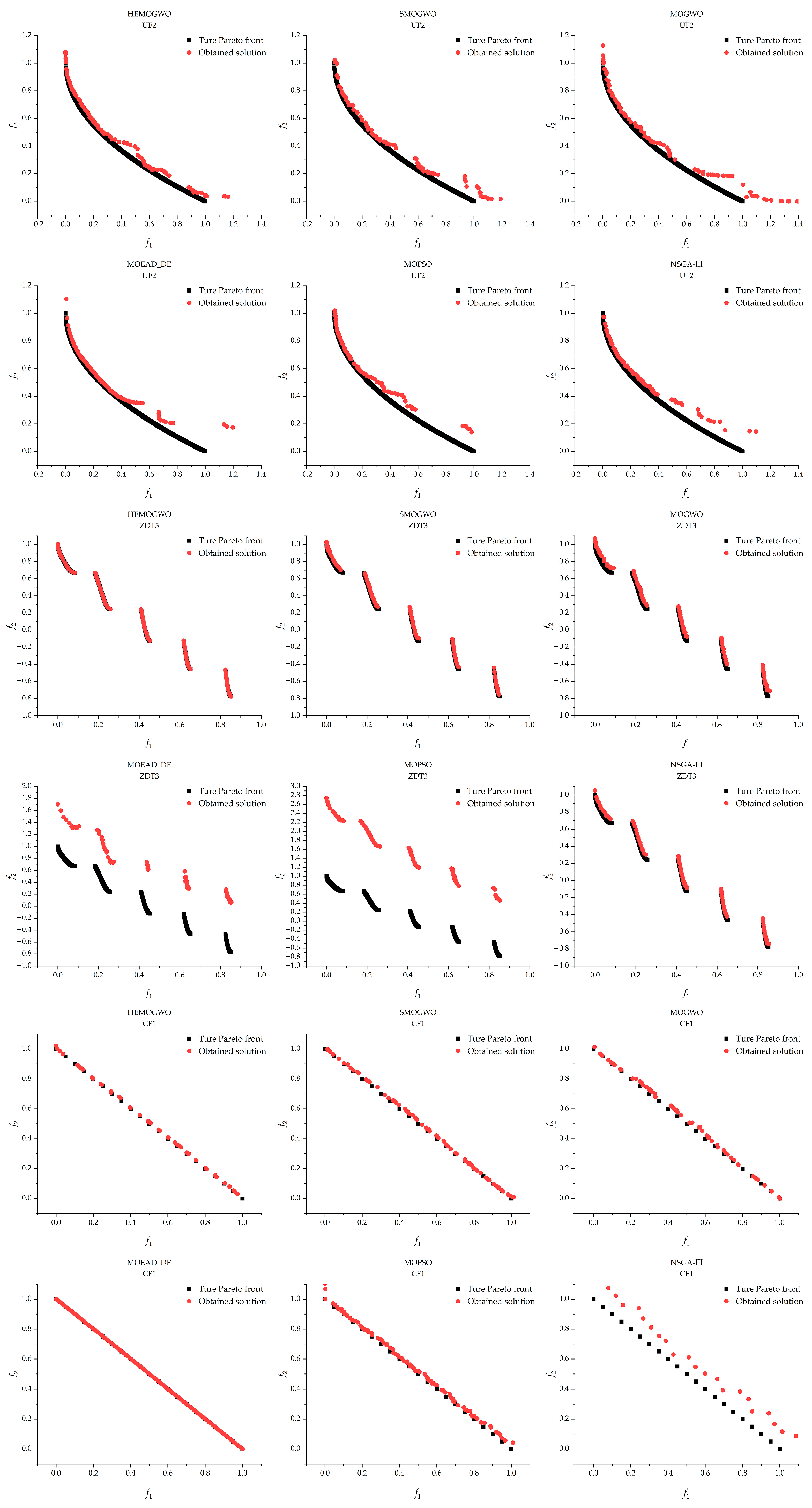
To provide a more intuitive comparison of the solution quality obtained by different algorithms, Figure 2 illustrates the optimal solution distributions of six algorithms on three representative benchmark functions: UF2, ZDT3, and CF1. In the plots, black solid squares represent the PF_ture, while red solid circles denote the sets of optimal solutions obtained by each algorithm. The visual analysis reveals that, on the UF2 function, HEMOGWO demonstrates superior convergence and solution set coverage compared to SMOGWO and MOGWO. This is particularly evident in the latter portion of the Pareto front, where the solution distribution of HEMOGWO aligns more closely with the true Pareto-optimal front. In contrast, SMOGWO and MOGWO exhibit noticeable deviations in certain regions, and their overall solution distributions are less uniform, indicating limitations in maintaining population diversity. For the ZDT3 function, HEMOGWO achieves full coverage of the PF_true, showcasing strong global search capability and distribution control, especially when dealing with the discontinuous PF structure. While SMOGWO, MOGWO, and NSGA-III follow the general trend, they still exhibit localized deviations. In comparison, the solution sets obtained by MOEAD_DE and MOPSO significantly diverge from PF_true, reflecting poor convergence and inconsistent distribution. On the CF1 function, MOEAD_DE performs the best, with its solutions closely matching PF_true and exhibiting the most uniform distribution among all compared algorithms.

To comprehensively evaluate the overall performance of each algorithm and establish a ranking, the GD and IGD results from Table 5 and Table 6 were subjected to the Friedman non-parametric test [30]. The test outcomes for both performance metrics are summarized in

Table 7. Friedman test results for GD and GD metrics on the benchmark functions (significant level is 0.05).

Metric	Algorithm	Mean Rank	Final Priority	N	df	Iman-Davenport F	p-Value
GD	HEMOGWO	1.41	1	17	(5, 80)	6.46 × 101	1.18 × 10−26
	SMOGWO	2.00	2
	MOGWO	2.76	3
	MOEAD_DE	4.71	5
	MOPSO	5.59	6
	NSGA-III	4.53	4
IGD	HEMOGWO	1.24	1			1.42 × 102	2.79 × 10−38
	SMOGWO	1.94	2
	MOGWO	2.82	3
	MOEAD_DE	4.82	5
	MOPSO	5.76	6
	NSGA-III	4.41	4

. As shown, the p-values for both GD and IGD are significantly lower than the predefined significance level of α = 0.05, indicating that the differences in performance among the five algorithms are statistically significant for both indicators. Furthermore, the rankings of the algorithms are consistent across the GD and IGD metrics, with HEMOGWO securing the first place in both cases. This demonstrates that HEMOGWO outperforms the other algorithms in terms of both convergence accuracy and solution distribution. These statistical findings are in strong agreement with the numerical results reported in Table 5 and Table 6.

The experimental results show that the HEMOGWO algorithm has better convergence and diversity in solving multi-objective problems, which proves the effectiveness of the improved strategy.

4.2. Case 2: The Performance of HEMOGWO on SCOS Problems

This section focuses on evaluating the performance of the proposed HEMOGWO algorithm in solving SCOS of varying scales. A real-world case from a printing equipment manufacturer in Shaanxi Province, China, serves as the application background. To advance its digital transformation, the enterprise aims to integrate five categories of core industrial software: ERP, MES, WMS, DCS, and PLM. Upon receiving the integration request, the platform decomposes it into five sub-tasks and performs service matching and composition. Assuming each sub-task has 20 candidate services, this scenario can be abstracted as a SCOS instance of scale “5-20”. Prior to computing the aggregated QoS metric, the weights for the four attributes—execution time, cost, reputation, and service quality—are uniformly set to 0.25. Parameter settings for all comparison algorithms are configured according to Table 4.

As the number of sub-tasks n and candidate services m increases, the solution space grows exponentially, imposing significant challenges on the algorithm’s global search capability and Pareto dominance handling. To further assess the generalizability and scalability of HEMOGWO, nine SCOS problem settings of different sizes are constructed: n ∈ {5, 10, 15} and m ∈ {20, 50, 100}, forming combinations such as 5-20, 5-50, 5-100, 10-20, 10-50, 10-100, 15-20, 15-50, and 15-100.

Given that no PF_true exists for real-world industrial composition optimization problems, this study adopts a widely used heuristic approximation method from existing research. Specifically, all algorithms are independently executed 30 times on each test instance, and the resulting solution sets are combined. A global non-dominated sorting is then applied to extract the set of globally optimal solutions, which is treated as the approximate PF_true. This approach maximizes coverage of the potential solution space and is extensively applied in multi-objective optimization research [8,9], effectively supporting fair performance evaluation across algorithms. To further validate the quality of the constructed PF_true, the distribution of solutions in the objective space is manually examined. Additionally, the consistency of GD and IGD metrics across algorithms confirms that the approximate PFtrue is both representative and reliable for comparative analysis.

The GD and IGD metrics are again used to evaluate convergence and distribution performance. To mitigate the influence of stochastic variations, each algorithm is independently executed 30 times. The mean and standard deviation of GD and IGD values are reported in

Table 8. Results of GD metric on SCOS problems.

Function		HEMOGWO	SMOGWO	MOGWO	MOEAD_DE	MOPSO	NSGA-III
5-20	Mean	1.30 × 10−3	1.53 × 10−3	1.77 × 10−3	4.41 × 10−3	7.04 × 10−3	2.53 × 10−3
	Std	8.77 × 10−4	3.60 × 10−4	4.41 × 10−4	5.06 × 10−4	9.37 × 10−4	2.68 × 10−3
5-50	Mean	2.48 × 10−3	2.67 × 10−3	4.62 × 10−3	1.20 × 10−2	1.32 × 10−2	4.34 × 10−3
	Std	1.12 × 10−3	3.53 × 10−3	1.73 × 10−3	1.45 × 10−3	1.61 × 10−3	4.50 × 10−4
5-100	Mean	3.03 × 10−3	8.10 × 10−3	1.21 × 10−2	2.24 × 10−2	2.24 × 10−2	9.04 × 10−3
	Std	2.59 × 10−3	2.87 × 10−3	1.92 × 10−3	6.79 × 10−3	6.77 × 10−3	4.97 × 10−3
10-20	Mean	1.77 × 10−2	1.17 × 10−2	1.79 × 10−2	4.15 × 10−2	5.54 × 10−2	2.09 × 10−2
	Std	5.72 × 10−2	6.55 × 10−2	5.96 × 10−2	6.80 × 10−2	9.14 × 10−2	7.17 × 10−2
10-50	Mean	4.35 × 10−2	5.71 × 10−2	4.00 × 10−2	7.05 × 10−2	1.02 × 10−1	2.11 × 10−2
	Std	2.33 × 10−3	1.22 × 10−2	1.74 × 10−2	2.26 × 10−2	2.91 × 10−2	2.35 × 10−3
10-100	Mean	7.89 × 10−2	1.31 × 10−1	1.66 × 10−1	1.44 × 10−1	2.19 × 10−1	1.38 × 10−1
	Std	2.02 × 10−2	3.31 × 10−2	3.29 × 10−2	4.07 × 10−2	5.06 × 10−2	3.62 × 10−2
15-20	Mean	3.10 × 10−2	4.05 × 10−2	5.03 × 10−2	9.05 × 10−2	1.33 × 10−1	4.75 × 10−2
	Std	1.28 × 10−2	1.70 × 10−2	1.14 × 10−2	2.65 × 10−2	3.49 × 10−2	1.11 × 10−2
15-50	Mean	7.86 × 10−2	7.90 × 10−2	6.41 × 10−2	1.26 × 10−1	1.73 × 10−1	9.27 × 10−2
	Std	4.61 × 10−2	2.62 × 10−2	3.08 × 10−2	2.75 × 10−2	3.80 × 10−2	4.64 × 10−2
15-100	Mean	7.42 × 10−2	1.03 × 10−1	1.34 × 10−1	2.24 × 10−1	2.88 × 10−1	1.18 × 10−1
	Std	2.12 × 10−2	2.57 × 10−2	2.78 × 10−2	5.34 × 10−2	6.11 × 10−2	2.47 × 10−2
+/≈/−			6/2/1	6/1/2	9/0/0	9/0/0	8/0/1

Bold indicates the best result under each indicator.

and

Table 9. Results of IGD metric on SCOS problems.

Function		HEMOGWO	SMOGWO	MOGWO	MOEAD_DE	MOPSO	NSGA-III
5-20	Mean	1.30 × 10−3	8.01 × 10−2	1.77 × 10−3	4.41 × 10−3	7.04 × 10−3	2.53 × 10−3
	Std	8.77 × 10−4	3.34 × 10−2	4.41 × 10−4	5.06 × 10−4	9.37 × 10−4	2.68 × 10−3
5-50	Mean	2.48 × 10−3	9.00 × 10−2	4.62 × 10−3	1.20 × 10−2	1.32 × 10−2	4.34 × 10−3
	Std	1.12 × 10−3	2.21 × 10−2	1.73 × 10−3	1.45 × 10−3	1.61 × 10−3	4.50 × 10−4
5-100	Mean	3.03 × 10−3	1.02 × 10−2	1.21 × 10−2	2.24 × 10−2	2.24 × 10−2	9.04 × 10−3
	Std	2.59 × 10−3	2.86 × 10−2	1.92 × 10−3	6.79 × 10−3	6.77 × 10−3	4.97 × 10−3
10-20	Mean	1.77 × 10−2	1.16 × 10−1	1.79 × 10−2	4.15 × 10−2	5.54 × 10−2	2.09 × 10−2
	Std	5.72 × 10−2	2.69 × 10−1	5.96 × 10−2	6.80 × 10−2	9.14 × 10−2	7.17 × 10−2
10-50	Mean	4.35 × 10−2	3.93 × 10−1	4.00 × 10−2	7.05 × 10−2	1.02 × 10−1	2.11 × 10−2
	Std	2.33 × 10−3	5.59 × 10−2	1.74 × 10−2	2.26 × 10−2	2.91 × 10−2	2.35 × 10−3
10-100	Mean	7.89 × 10−2	9.10 × 10−1	1.66 × 10−1	1.44 × 10−1	2.19 × 10−1	1.38 × 10−1
	Std	2.02 × 10−2	7.25 × 10−2	3.29 × 10−2	4.07 × 10−2	5.06 × 10−2	3.62 × 10−2
15-20	Mean	3.10 × 10−2	1.11 × 10−1	5.03 × 10−2	9.05 × 10−2	1.33 × 10−1	4.75 × 10−2
	Std	1.28 × 10−2	7.31 × 10−2	1.14 × 10−2	2.65 × 10−2	3.49 × 10−2	1.11 × 10−2
15-50	Mean	7.86 × 10−2	4.22 × 10−1	6.41 × 10−2	1.26 × 10−1	1.73 × 10−1	9.27 × 10−2
	Std	4.61 × 10−2	2.70 × 10−1	3.08 × 10−2	2.75 × 10−2	3.80 × 10−2	4.64 × 10−2
15-100	Mean	7.42 × 10−2	7.11 × 10−1	1.34 × 10−1	2.24 × 10−1	2.88 × 10−1	1.18 × 10−1
	Std	2.12 × 10−2	7.81 × 10−2	2.78 × 10−2	5.34 × 10−2	6.11 × 10−2	2.47 × 10−2
+/≈/−			6/2/1	8/0/1	9/0/0	9/0/0	8/0/1

Bold indicates the best result under each indicator.

, respectively. For clarity, the best-performing values in each metric are highlighted in bold. According to the statistical results, HEMOGWO consistently outperforms the competing algorithms across various problem scales. The specific analysis is as follows.

Table 8 and Table 9 present the GD and IGD results of all algorithms, respectively, for evaluating their overall distribution performance. The statistical results indicate that the HEMOGWO algorithm achieves the best performance in terms of the GD metric across the majority of tested problem scales. However, in certain small- to medium-scale scenarios—such as 10-20, 10-50, and 15-50—its GD mean values are higher than those of competing algorithms, and its standard deviations are also relatively larger. This suggests that, in these specific cases, HEMOGWO does not exhibit superior convergence accuracy or stability. As the problem scale increases, particularly in medium-to-large configurations like 10-100 and 15-100, HEMOGWO once again demonstrates a clear advantage, producing solution sets that more closely approximate the true Pareto front and exhibit greater consistency. In contrast, SMOGWO, MOGWO, and NSGA-III display competitive performance only under limited scales, with less consistent results overall. Regarding the IGD metric, HEMOGWO maintains a dominant position. Except for three problem scales (5-100, 10-100, and 15-50), it achieves the lowest IGD mean values in all other test scenarios. Notably, in small-scale problems such as 5-20 and 10-20, HEMOGWO significantly outperforms all baseline algorithms, highlighting its superior ability in maintaining balanced solution set distributions. Moreover, the standard deviation analysis shows that HEMOGWO generally exhibits lower variability across most problem scales, further validating its robustness and algorithmic stability. In comparison, MOPSO performs worst in terms of IGD. It frequently suffers from poor convergence and solution sets that deviate from the Pareto front, likely due to its tendency to become trapped in local optima and its limited capacity to maintain population diversity.

The WSRT results based on GD and IGD metrics indicate that HEMOGWO achieved a complete win against MOEAD_DE and MOPSO in terms of GD, demonstrating a significant advantage in the accuracy of approximating the true Pareto front. When compared with NSGA-III, HEMOGWO attained a favorable result of 8/0/1, showing only a marginal performance gap in one test scenario. Although a few ties and isolated losses were observed in comparisons with SMOGWO and MOGWO, HEMOGWO still secured six wins in both cases, indicating superior overall performance. Regarding the IGD metric, HEMOGWO also exhibited strong distribution capability. Except for one loss and two ties against SMOGWO, it achieves a decisive victory in all comparisons with MOGWO, MOEAD_DE, MOPSO, and NSGA-III, particularly securing a perfect record in the comparisons with MOEAD_DE and MOPSO.

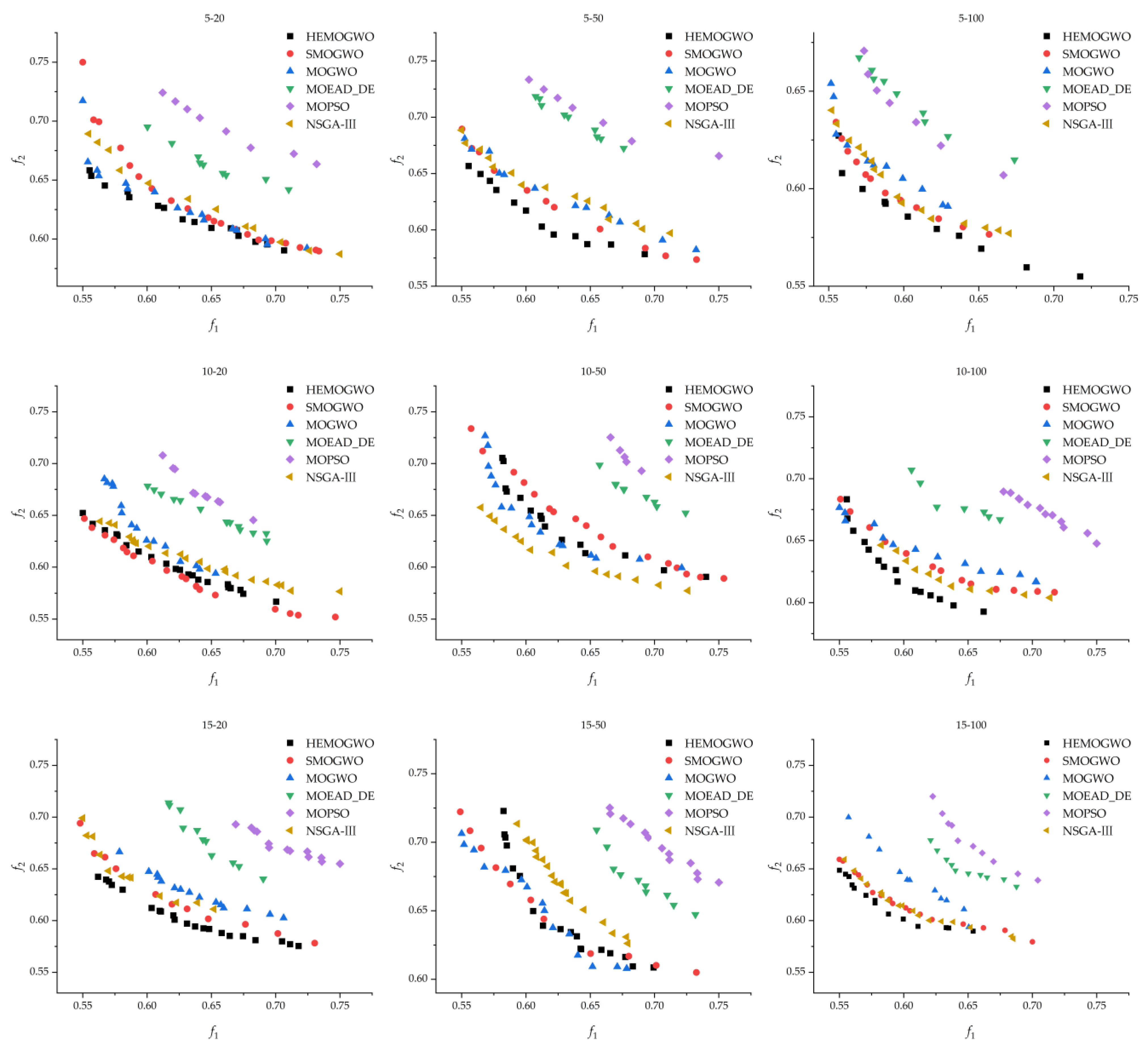
To provide an intuitive comparison of the optimization performance of each algorithm on SCOS problems, Figure 3 shows the distribution of Pareto-optimal solutions under different problem scales after normalization. From the distribution patterns, it is evident that the optimal solutions obtained by the HEMOGWO algorithm are mainly concentrated along the outer boundary of the true Pareto front. This suggests its significant advantage in convergence, demonstrating its ability to effectively approximate the global optimal front. The results confirm HEMOGWO’s strong capability to balance solution diversity with proximity to the true Pareto front. SMOGWO and NSGA-III exhibit a nondominated solution set with a distribution pattern similar to that of HEMOGWO. The uniformity and coverage of their solutions further highlight the algorithm’s adaptability and effectiveness in solving complex SCOS scenarios. In contrast, the solution sets generated by MOPSO and MOEAD_DE show clear deviations from the true Pareto front, with this divergence becoming more pronounced as the problem scale increases.

Table 10. Friedman test results for GD and IGD metrics on the SCOS problems (significant level is 0.05).

Metric	Algorithm	Mean Rank	Final Priority	N	df	Iman-Davenport F	p-Value
GD	HEMOGWO	1.44	1	9	(5, 40)	3.32 × 101	3.21 × 10−13
	SMOGWO	2.22	2
	MOGWO	3.33	4
	MOEAD_DE	4.94	5
	MOPSO	5.94	6
	NSGA-III	3.11	3
IGD	HEMOGWO	1.44	1			5.11 × 101	2.59 × 10−16
	SMOGWO	2.00	2
	MOGWO	3.44	4
	MOEAD_DE	5.0000	5
	MOPSO	6.0000	6
	NSGA-III	3.11	3

presents the Friedman test rankings of the compared algorithms based on the GD and IGD performance indicators. The results indicate that the HEMOGWO algorithm achieved the highest rank on both metrics, significantly outperforming the other compared algorithms. This strongly supports its superior overall performance in solving multi-objective optimization problems. SMOGWO ranked second in both GD and IGD, demonstrating its strong competitiveness in handling complex multi-objective tasks, particularly in balancing convergence and solution distribution. MOGWO ranked fourth, suggesting that while it inherits strengths from the original gray wolf optimizer, it is slightly inferior to HEMOGWO and SMOGWO in terms of convergence accuracy and solution diversity. In contrast, MOEAD_DE and MOPSO ranked fifth and sixth, respectively, reflecting clear limitations in convergence speed, solution uniformity, and proximity to the true Pareto front. Notably, the rankings across GD and IGD were highly consistent for all algorithms, further confirming the complementarity and reliability of these two metrics in evaluating multi-objective optimization performance. Finally, all p-values from the tests were well below the 0.05 threshold, providing strong evidence of statistically significant performance differences among the algorithms.

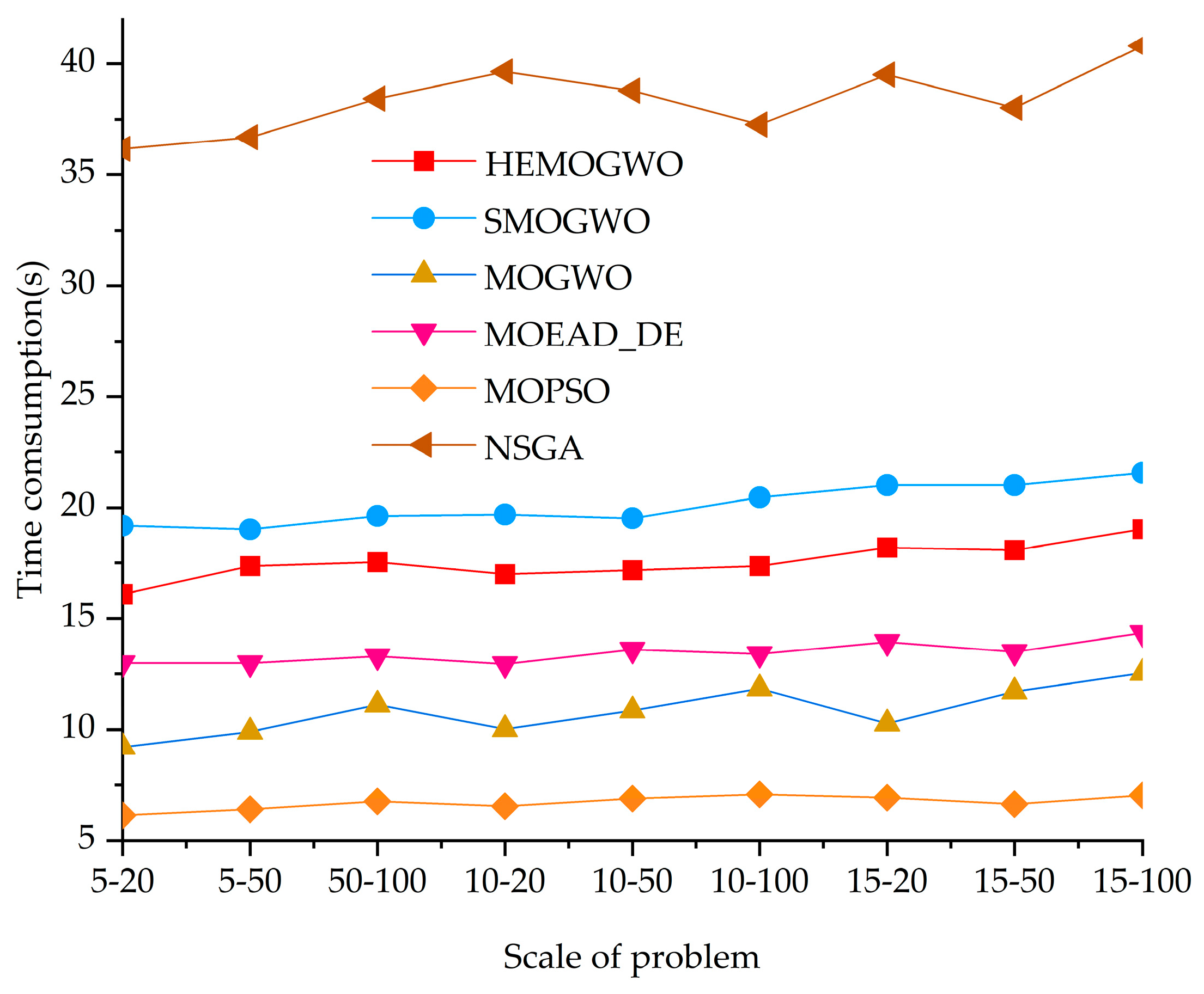
Finally, to quantitatively assess the computational cost of each algorithm across varying scales of SCOS problems, this study presents a statistical analysis of their runtime, as illustrated in Figure 4. The experimental results show that MOPSO consistently exhibits the highest computational efficiency across all test scales, with runtimes significantly lower than those of the other algorithms. This efficiency is primarily attributed to its simple and effective particle update mechanism. MOGWO and MOEAD_DE also demonstrate slightly lower runtimes compared to HEMOGWO, indicating relatively lower computational complexity. In contrast, the HEMOGWO algorithm, due to the incorporation of a hybrid differential evolution strategy enhanced by chaotic mapping and Lévy flight mechanisms, involves a more sophisticated search process, resulting in relatively higher computational costs. However, when considered alongside the GD and IGD performance metrics, HEMOGWO clearly outperforms the other algorithms in terms of solution accuracy and stability. Although its runtime exceeds that of MOGWO, MOEAD_DE, and MOPSO, the additional computational cost remains within a reasonable and acceptable range for practical applications that demand high-quality solutions. Notably, although SMOGWO and NSGA-III exhibit performance levels close to that of HEMOGWO, their execution times are significantly longer. In particular, the average computational cost of NSGA-III is approximately three times that of HEMOGWO, which limits its applicability in resource-constrained environments.

5. Discussion

The performance of the proposed HEMOGWO algorithm was systematically evaluated through empirical studies on both a set of standard multi-objective test functions and a real-world industrial task from the SCOS software system. In terms of the two key performance metrics, GD and IGD, HEMOGWO outperformed SMOGWO, NSGA-III, MOEAD_DE, MOPSO, and the original MOGWO. It consistently ranked first in the Friedman test, indicating statistically significant advantages in solution accuracy, distribution uniformity, and stability.

Further analysis reveals that the Tent chaotic mapping strategy effectively improved the spatial coverage of the population during the initialization phase, laying a solid foundation for subsequent optimization. The Lévy flight mechanism enhanced the algorithm’s global exploration capability and its ability to escape local optima. Additionally, the integration of the differential evolution operator improved local search precision in the later stages, significantly enhancing the concentration and convergence speed of the solution set. These enhancements demonstrated strong adaptability in the SCOS task, meeting the dual industrial requirements of system stability and service availability.

Although the proposed method outperforms other algorithms in most tasks, the integration of complex evolutionary mechanisms has led to a slight increase in per-unit runtime. Nevertheless, from the perspective of overall optimization performance and industrial applicability, this computational overhead remains within an acceptable range, confirming the effectiveness of the algorithm in addressing real-world complex optimization problems.

However, although this study incorporated real-world parameters and extended them based on their distributions to improve the representativeness and controllability of the experimental data, certain limitations remain. The current dataset primarily focuses on static modeling at the level of service parameters and does not adequately reflect the dynamic behaviors present in real industrial service composition processes. Therefore, the experimental results partially demonstrate the algorithm’s optimization performance under idealized conditions and require further validation in actual industrial workflows or dynamic service environments.

6. Conclusions and Future Works

This study addresses the integration and composition optimization challenges of industrial software systems operating in heterogeneous environments. To tackle issues such as insufficient reliability and difficulty in balancing QoS during service selection, a bi-objective optimization model is proposed. The model comprehensively considers service time, cost, reputation, delivery quality, and availability. Service availability is quantified using MTBF and MTTR, while service dependencies and integration uncertainties are incorporated to construct a service optimization framework suitable for multi-source heterogeneous systems.

Building on this model, a set of coordinated strategies—namely chaotic initialization, differential evolution, and Lévy flight mechanisms—is introduced to enhance the quality, stability, and convergence efficiency of multi-objective optimization in industrial software service composition. Based on these strategies, the HEMOGWO algorithm is developed. It integrates Tent chaotic mapping to improve population diversity, incorporates an improved differential evolution operator to enhance local precision, and applies a Lévy flight-based mechanism to strengthen global search capability.

To verify the effectiveness of the proposed method, a dual experimental framework was designed, incorporating both standard benchmark functions and real-world industrial tasks. The performance of HEMOGWO was compared against several mainstream multi-objective algorithms, including NSGA-III, MOPSO, MOEAD_DE, MOGWO, and its improved variant, SMOGWO. The results show that HEMOGWO achieved the best performance in terms of GD and IGD metrics on most benchmark functions. For nine types of SCOS-based real-world composition optimization tasks, HEMOGWO also obtained the lowest mean GD and IGD values across the majority of test scales. Its superiority was further confirmed through the Wilcoxon signed-rank test, particularly in terms of improved solution accuracy and computational speed compared with SMOGWO.

The main contributions of this study are as follows: (1) a bi-objective SCOS model integrating QoS and availability is proposed, introducing system-level availability modeling into industrial software service composition optimization for the first time; (2) a HEMOGWO algorithm incorporating multiple intelligent search mechanisms is developed, and its performance advantages are validated; and (3) a combined testing framework based on standard benchmark functions and industrial scenarios is designed to comprehensively evaluate the algorithm’s generalization ability and practical applicability.

Certainly, this study has several limitations. First, the experimental dataset is primarily constructed based on real-world parameter distributions but does not capture dynamic behavioral dependencies or real-time interaction logic among services. Second, the service composition process is modeled statically, without accounting for practical constraints such as multi-user requests, service fluctuations, and resource contention. Moreover, the balance between real-time performance and computational complexity in the proposed algorithm requires further optimization.

Future research can address these issues in several ways—by introducing log-driven dynamic workflow modeling to enhance the realism of test data; by extending HEMOGWO to dynamic environments and multi-tenant service scheduling tasks; and by exploring its online deployment capability and engineering implementation within industrial cloud platforms. These efforts aim to promote the algorithm’s broader application in intelligent manufacturing scenarios.

References

1. Gao, T.; Wang, L.; Song, W. Ten industrial software towards smart manufacturing. J. Manuf. Syst. 2025, 79, 255–285. [Google Scholar] [CrossRef]
2. Barkat, A.; Kazar, O.; Seddiki, I. Framework for web service composition based on QoS in the multi cloud environment. Int. J. Inf. Technol. 2021, 13, 459–467. [Google Scholar] [CrossRef]
3. Gao, B.; Wang, S.; Kang, L. Diagnosis and handling of exception in cloud manufacturing. In Proceedings of the 2018 Prognostics and System Health Management Conference (PHM-Chongqing), Chongqing, China, 26–28 October 2018; IEEE: Piscataway, NJ, USA, 2018; pp. 866–870. [Google Scholar]
4. Yang, B.; Wang, S.; Li, S. A robust service composition and optimal selection method for cloud manufacturing. Int. J. Prod. Res. 2022, 60, 1134–1152. [Google Scholar] [CrossRef]
5. Zhao, Z.; Zhou, H.; Wang, X.; Hua, X. Enhancing reconfiguration of cloud manufacturing service composition under unexpected changes in service time availability by flexible splitting and intermingling strategies. Robot. Comput.-Integr. Manuf. 2025, 95, 103044. [Google Scholar] [CrossRef]
6. Yang, B.; Wang, S.; Li, S.; Bi, F. Digital Thread-Driven Proactive and Reactive Service Composition for Cloud Manufacturing. IEEE Trans. Ind. Inform. 2023, 19, 2952–2962. [Google Scholar] [CrossRef]
7. Yin, C.; Li, S. An adaptive adjustment method for cloud service exception based on grey correlation analysis. Manuf. Autom. 2023, 45, 197–202+211. [Google Scholar]
8. Gao, Y.; Yang, B.; Wang, S. Bi-objective service composition and optimal selection for cloud manufacturing with QoS and robustness criteria. Appl. Soft Comput. 2022, 128, 109530. [Google Scholar] [CrossRef]
9. Zhang, Q.; Li, S.; Pu, R. An adaptive robust service composition and optimal selection method for cloud manufacturing based on the enhanced multi-objective artificial hummingbird algorithm. Expert Syst. Appl. 2024, 244, 122823. [Google Scholar] [CrossRef]
10. Mai, L.; Ding, Y.; Zhang, X. Energy efficiency with service availability guarantee for Network Function Virtualization. Future Gener. Comput. Syst. 2021, 119, 140–153. [Google Scholar] [CrossRef]
11. Ni, H.; Yan, C.; Chen, J. Multi-objective Optimization and Decision-making Method of High Speed Dry Gear Hobbing Processing Parameters. China Mech. Eng. 2021, 32, 832–838. [Google Scholar]
12. Xue, S.; Xie, X.; Zhen, X. Adaptive denoising for leak-induced acoustic in gas pipe under multiple conditions. Chin. J. Sci. Instrum. 2024, 45, 227–239. [Google Scholar]
13. Liu, J.; Yang, Z.; Li, D. A multiple search strategies based grey wolf optimizer for solving multi-objective optimization problems. Expert Syst. Appl. 2020, 145, 113134. [Google Scholar] [CrossRef]
14. Wynn, S.; Pinthurat, W.; Marungsri, B. Multi-objective optimization for peak shaving with demand response under renewable generation uncertainty. Energies 2022, 15, 8989. [Google Scholar] [CrossRef]
15. Dong, J.; Ye, C. Research on collaborative optimization of green manufacturing in semiconductor wafer distributed heterogeneous factory. Appl. Sci. 2019, 9, 2879. [Google Scholar] [CrossRef]
16. Chen, H.; Yu, P.; Long, J. Multi-objective optimization of automotive seat frames using machine learning. Adv. Eng. Softw. 2025, 199, 103797. [Google Scholar] [CrossRef]
17. Nadimi-Shahraki, M.; Taghian, S.; Mirjalili, S. An improved grey wolf optimizer for solving engineering problems. Expert Syst. Appl. 2021, 166, 113917. [Google Scholar] [CrossRef]
18. Yin, C.; Xu, J.; Li, X. NSGA-III based service composition optimization method in cloud manufacturing. Comput. Integr. Manuf. Syst. 2022, 28, 1164–1176. [Google Scholar]
19. Que, Y.; Zhong, W.; Chen, H. Improved adaptive immune genetic algorithm for optimal QoS-aware service composition selection in cloud manufacturing. Int. J. Adv. Manuf. Technol. 2018, 96, 4455–4465. [Google Scholar] [CrossRef]
20. Yang, Y.; Yang, B.; Wang, S. An improved grey wolf optimizer algorithm for energy-aware service composition in cloud manufacturing. Int. J. Adv. Manuf. Technol. 2019, 105, 3079–3091. [Google Scholar] [CrossRef]
21. Yang, P.; Qiu, J.; Liu, G. Testability index determination method based on ROM model. Acta Aeronaut. Astronaut. Sin. 2021, 42, 273–286. [Google Scholar]
22. Mirjalili, S.; Saremi, S.; Mirjalili, S. Multi-objective grey wolf optimizer, a novel algorithm for multi-criterion optimization. Expert Syst. Appl. 2016, 47, 106–119. [Google Scholar] [CrossRef]
23. Mirjalili, S.; Mirjalili, S.; Lewis, A. Grey wolf optimizer. Adv. Eng. Softw. 2014, 69, 46–61. [Google Scholar] [CrossRef]
24. Zhang, Q.; Liu, H.; Guo, J.; Wang, Y.; Liu, L.; Liu, H.; Cong, H. Improved GWO-MCSVM algorithm based on nonlinear convergence factor and tent chaotic mapping and its application in transformer condition assessment. Electr. Power Syst. Res. 2023, 224, 109754. [Google Scholar] [CrossRef]
25. Zeng, Z.; Zhang, M.; Chen, T. A new selection operator for differential evolution algorithm. Knowl.-Based Syst. 2021, 226, 107150. [Google Scholar] [CrossRef]
26. Liu, M.; Yao, X.; Li, Y. Hybrid whale optimization algorithm enhanced with Lévy flight and differential evolution for job shop scheduling problems. Appl. Soft Comput. 2020, 87, 105954. [Google Scholar] [CrossRef]
27. Nunes, I.; Araújo, M.; Lopez, J. Frequency redistribution and step-size distribution of light scattered by atomic vapor, applications to Lévy flight random walk. arXiv 2024, arXiv:2411.18570. [Google Scholar] [CrossRef]
28. Gao, Z.; Liu, S.; Qian, S. A Resource Composition Optimization Algorithm Based on Improved Polar Bear Optimization Algorithm for Manufacturing Wallboard for Coating Machine. Coatings 2025, 15, 418. [Google Scholar] [CrossRef]
29. Derrac, J.; García, S.; Molina, D. A practical tutorial on the use of nonparametric statistical tests as a methodology for comparing evolutionary and swarm intelligence algorithms. Swarm Evol. Comput. 2011, 1, 3–18. [Google Scholar] [CrossRef]
30. De, C.; Özcan, E.; Sichman, J. Comparative analysis of selection hyper-heuristics for real-world multi-objective optimization problems. Appl. Sci. 2021, 11, 9153. [Google Scholar]
Figure 1. Schematic diagram of SCOS.
Applsci 15 07754 g001
Figure 2. Results of all algorithms on benchmark function UF2,ZDT3, and CF1.
Applsci 15 07754 g002
Figure 3. The best solution distribution.
Applsci 15 07754 g003
Figure 4. Comparison of time consumption of different algorithms.
Applsci 15 07754 g004