Real-Time Image Analysis for Intelligent Aircraft De-Icing Decision Support Systems

Abstract

Aircraft icing and snow accumulation are significant threats to flight safety and operational efficiency, necessitating rapid and accurate detection methods. The aim of this study was to develop and comparatively evaluate artificial intelligence (AI) models for the real-time detection of ice and snow on aircraft surfaces using vision systems. A custom dataset of annotated aircraft images under various winter conditions was prepared and augmented to enhance model robustness. Two training approaches were implemented: an automatic process using the YOLOv8 framework on the Roboflow platform and a manual process in the Google Colab environment. Both models were evaluated using standard object detection metrics, including mean Average Precision (mAP) and mAP@50:95. The results demonstrate that both methods achieved comparable detection performance, with final mAP50 values of 0.25–0.3 and mAP50-95 values around 0.15. The manual approach yielded lower training losses and more stable metric progression, suggesting better generalization and a reduced risk of overfitting. The findings highlight the potential of AI-driven vision systems to support intelligent de-icing decision-making in aviation. Future research should focus on refining localization, minimizing false alarms, and adapting detection models to specific aircraft components to further enhance operational safety and reliability.

1. Introduction

The problem of aircraft icing and snow accumulation is one of the most serious challenges facing modern aviation. It directly affects both operational safety and economic efficiency. Ice on aerodynamic surfaces, such as wings or stabilizers, disrupts airflow, leading to reduced lift, increased aerodynamic drag, and difficulties in controlling the aircraft. Icing can also increase the aircraft’s weight, shift its center of gravity, and block the operation of systems such as control surfaces, brakes, or sensors. In extreme cases, this can lead to loss of control of the aircraft. Additionally, ice on windshields reduces visibility, posing an additional hazard during takeoff and landing. During takeoff, icing lengthens the takeoff run and increases the risk of stalling, while during flight, conditions involving freezing rain or drizzle are particularly dangerous, as they can quickly create a thick layer of ice that is difficult to remove [1,2,3]. Snow in aviation is less problematic than ice, but it can still negatively affect the organization of flight operations. Dry snow usually does not adhere permanently to the aircraft’s surface, while wet snow at temperatures between 0 °C and 5 °C can quickly turn into ice on the airframe, creating hazards. Additionally, heavy snowfall can reduce visibility and make takeoffs and landings more difficult. Regardless of the type of snow (safe or dangerous), safety procedures are undertaken to remove it. The risk of snow accumulation and icing depends on the region of the world. Regions particularly at risk of icing and snow accumulation are primarily polar areas, such as the Arctic and Antarctic, where extreme weather conditions are common. However, problematic weather conditions affect many regions around the world [4,5,6].

Icing has been the cause of many aviation disasters over the years. Examples include the crash of a Boeing 721 in Iran in 2011 and the tragic accident of Fuerza Aérea Uruguaya Flight 571 in the Andes in 1972. These events highlight the importance of effective anti-icing methods for aviation safety [7,8]. Modern anti-icing methods include both traditional mechanical and chemical procedures as well as innovative technologies. Vision systems enable the rapid detection of ice or snow on aircraft surfaces and support real-time de-icing decisions. Advanced solutions use optical sensors and image analysis algorithms to provide detailed information about the aircraft’s condition [9].

Vision systems are increasingly supported by artificial intelligence models [10]. Therefore, an attempt was made to develop an artificial intelligence (AI) model capable of automatically recognizing snow and ice on aircraft surfaces. This process required creating an appropriate training dataset and training the model based on various weather scenarios and operational conditions. Currently, there is no ready-made AI model dedicated to this purpose, which makes this task particularly ambitious and innovative. Developing such a solution could significantly improve the effectiveness of ice detection and the optimization of de-icing procedures, thereby contributing to increased aviation safety and operational efficiency in challenging weather conditions. At present, these are preliminary studies and will be further developed in the future [11,12].

2. Literature Review

Aircraft icing constitutes one of the most serious threats to flight safety, affecting aerodynamics, aircraft mass, and the functioning of key onboard systems. Intelligent decision support systems based on real-time image analysis can significantly improve the effectiveness of de-icing procedures, minimizing the associated operational risk. The literature provides extensive information on aircraft icing, its causes, and its consequences for the safety of flight operations. Intensive research on this phenomenon began in the 1980s, when NASA, in response to the crash of an Air Florida Boeing 737 in 1982, initiated a comprehensive research program using a De Havilland DH-6 Twin Otter aircraft as a test platform. Initially, the research focused on measuring the properties of icing clouds, and then expanded the analysis to include the impact of icing on aircraft performance, using, among other things, stereophotography to document ice shapes on wings and the analysis of aerodynamic losses. The Flight Safety Foundation and the University of British Columbia published detailed studies on the mechanisms of icing formation and its impact on flight safety, highlighting the key role of supercooled water droplets occurring at temperatures from 0 °C to −40 °C. Contemporary research, conducted by institutions such as the AOPA Air Safety Institute and the FAA, provides valuable information on the effectiveness of anti-icing systems and operational strategies minimizing the risks associated with this phenomenon [13,14].

Aircraft icing leads to serious aerodynamic consequences that directly affect flight safety. The primary mechanism is the disruption of airflow around the airframe, which results in increased aerodynamic drag and a simultaneous decrease in lift. Even a thin layer of ice, about 60 mm (1/4 inch) thick, can significantly impact the aerodynamic characteristics of the aircraft, increasing drag by as much as 40 to 80% and requiring a higher angle of attack and greater speed to maintain flight. As a result, an aircraft with iced surfaces stalls at higher speeds and behaves unpredictably. Icing also increases the aircraft’s mass and can shift its center of gravity, further complicating control of the aircraft. Particularly dangerous is tailplane icing, which can lead to so-called tail stall and sudden nose-down pitching of the aircraft. In the case of engines, icing of air intakes or carburetors leads to power loss or complete failure, which poses a direct threat to the continuation of the flight.

Aircraft icing is classified according to various criteria, taking into account both the location and the characteristics of the ice formed. The basic division includes structural icing (affecting the external surfaces of the aircraft) and induction icing (related to engine systems) [15,16,17].

Within structural icing, several characteristic types of ice can be distinguished. Clear ice forms at temperatures from 0 °C to −5 °C and is characterized by a smooth, transparent structure that significantly increases aerodynamic drag and is difficult to remove. Rime ice, which forms at temperatures below −10 °C, has a porous, milky-white structure that disrupts airflow, although it is easier to remove. Mixed ice is a combination of both types and occurs at temperatures from −5 °C to −10 °C, creating irregular, uneven deposits that are particularly dangerous for the aircraft’s aerodynamics. Hoar frost forms as a result of the direct deposition of water vapor on cold surfaces and, although it does not radically change the shape of the wings, it reduces lift by up to 30% and increases drag by 40%. Wet snow poses an additional threat, as it contains water particles that can freeze on aircraft surfaces, while dry snow usually does not cause icing [14,18,19].

Effective prevention of icing requires an integrated approach that combines appropriate technical systems with operational procedures. Anti-icing systems are designed to prevent the accumulation of ice on critical aircraft surfaces by heating them (using hot air from the engines) or by applying special chemical fluids (e.g., TKS Fluid). For carbureted engines, it is crucial to use carburetor heating, especially when reducing engine power, as this prevents ice formation in the intake system even at temperatures reaching 25 °C. Another important element of icing prevention is proper flight planning, taking into account weather forecasts and PIREP, SIGMET, and AIRMET reports, which provide information about potential icing risks along the planned route. Pilots should avoid areas with a high risk of supercooled water, especially in low clouds (up to 6500 feet above ground) and in the temperatures range from 0 °C to −40 °C. In the case of aircraft not equipped with appropriate anti-icing systems, it is essential to avoid icing-prone conditions by changing flight altitude or route. Removing already formed ice requires the use of specialized techniques and systems. De-icing systems differ from anti-icing systems in that they are used to remove existing ice, not to prevent its formation. In commercial aviation, de-icing fluids are commonly used before takeoff to dissolve existing ice deposits and provide temporary protection against re-icing. Onboard the aircraft, various mechanical systems are used, such as pneumatic “boots” on wing leading edges, which, through cyclic inflation and deflation, break and remove ice deposits. Newer designs use electric heating systems on critical surfaces to melt accumulating ice. An innovative approach is the use of durable superhydrophobic coatings on composite surfaces, which minimize ice adhesion by reducing water adhesion and delaying the freezing process. Studies have shown that these coatings can reduce ice adhesion by up to 80% compared to uncoated surfaces, maintaining their properties for over 500 freeze–thaw cycles. The combination of passive superhydrophobic coatings with active de-icing methods allows energy consumption to be reduced by up to 40%, which is economically and environmentally significant [20,21,22].

The effective mitigation of icing-related hazards requires strict adherence to specific operational procedures. The fundamental principle is the “clean wing”—before takeoff, all ice or snow deposits must be thoroughly removed from the aircraft’s surfaces, as even a thin layer of frost can prevent a safe takeoff. During flight, it is crucial to monitor airspeed as an indicator of potential icing—a gradual decrease at constant engine power may signal increasing ice accumulation. On approach, in the case of icing, it is recommended to increase the final approach speed by 10–20 knots and avoid full flap extension, which reduces the risk of stalling. If icing conditions are encountered, pilots should immediately leave the area by changing altitude or course and report the situation to air traffic control. For carbureted engines, it is important to use carburetor heating prophylactically, in accordance with the operating manual. Icing of rotating blades requires special attention—pilots should recognize early signs of tailplane stall, such as unusual stick forces and control column vibrations. Ground personnel responsible for de-icing should use appropriate fluids and techniques, taking into account weather conditions and the expected departure time [23,24,25].

Modern approaches to ice prevention increasingly rely on advanced vision technologies and real-time image analysis to objectively assess aircraft surface conditions, surpassing traditional visual inspections. These systems use multispectral cameras (visible, infrared, UV) to detect ice type (clear, rime, mixed) and measure thickness. Integration with machine learning algorithms enables AI-driven decision support systems that recommend optimal de-icing methods, fluid types, and durations based on real-time ice conditions and weather data. This approach reduces resource waste and delays while enhancing safety. Future solutions will likely combine vision systems with plasma technologies and automated fluid application systems, guided by AI analyzing real-time sensor data. Hybrid systems aim to improve energy efficiency and responsiveness to icing threats [26,27,28].

There are vision systems for detecting aircraft icing and snow. One such system is a model based on DETR (Detection Transformer) technology, which has been applied to detect icing and snow on aircraft surfaces. This system uses self-attention mechanisms, allowing for precise analysis of spatial relationships between ice, snow, and the structure of the aircraft. To improve the precision of icing boundary localization, an additional RefineBox optimization network was used. Studies conducted on a custom image dataset demonstrated the high effectiveness of this system in various environmental conditions, such as different lighting angles or the presence of clear ice and icicles. This model achieved a high detection accuracy, making it a promising tool for practical operational use at airports. Another approach is the use of laser systems for detecting and removing ice. This technology uses laser radiation at a wavelength that is preferentially reflected by the aircraft surface but absorbed by ice, snow, and water. This enables precise monitoring of surface temperature and identification of areas covered with ice. The system also allows for mapping the thickness of the ice and documenting its location using thermal cameras. These technologies can be used both for detection and real-time removal of ice [29].

Another example is the Smart Ice Control System based on machine learning, which utilizes various artificial intelligence models such as logistic regression, support vector machines (SVM), and neural networks (Multilayer Perceptron). This system analyzes data from temperature and humidity sensors to predict ice formation in real time. By employing supervised and unsupervised learning algorithms, it enables not only precise ice detection but also optimization of de-icing processes, enhancing operational safety and reducing energy consumption [30].

Intelligent Vision Systems (IVSs) technology uses diffuse light imaging and artificial intelligence to instantly detect ice both in the air and on the ground. This system enables the identification of ice crystals and snow located beneath the surface being de-iced before takeoff. This technology supports pilots in making operational decisions and helps aircraft manufacturers meet regulatory requirements for ice detection [31].

Vision systems used in aviation can be significantly enhanced by artificial intelligence (AI), especially in the context of detecting snow and ice on aircraft surfaces. AI models, based on machine learning algorithms, have the potential to automatically recognize snow coverage, identify its type, and assess the degree of threat to flight operations. However, building such a model requires considerable effort, starting with collecting a sufficiently large training dataset that includes images of aircraft in various weather conditions, followed by their detailed analysis and labeling. It is also crucial to take into account the variability of lighting conditions, camera angles, and the diversity of snow types. The author of this article undertakes the challenge of developing such an AI model, being aware of its complexity, but at the same time recognizing the enormous potential that the use of artificial intelligence brings to de-icing decision-making processes. With a properly trained AI model, it will be possible to increase the precision of snow detection on aircraft and optimize de-icing procedures, which will contribute to improved flight safety and operational efficiency in aviation [32,33].

3. Research Methodology

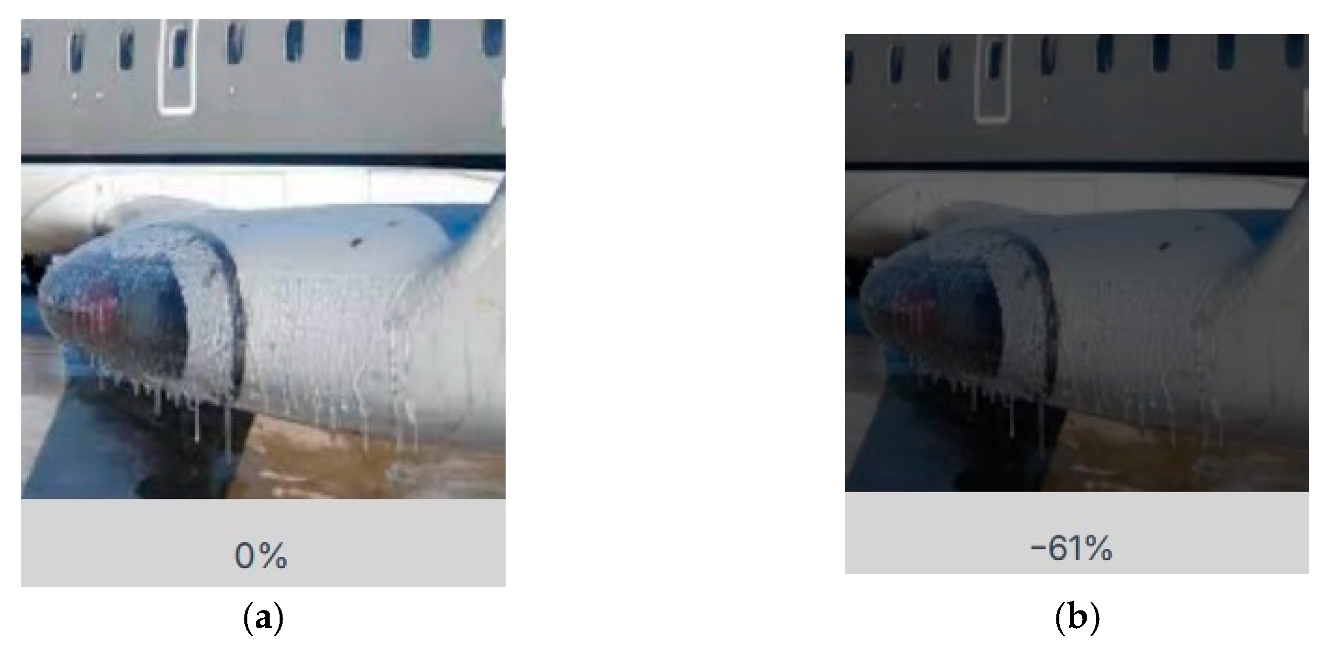
The research process began with the collection and preparation of aerial photographs. The images were sourced from publicly available online resources. In Poland, regulations prohibiting the photographing of military objects, bridges, and airports were introduced on 17 August 2023. Therefore, the author of the study used photographs found on the internet. The images in the dataset depicted airplanes in winter conditions, showing varying degrees of icing and snow coverage. Preliminary results from previous research indicated that object classification depends on light intensity, dominant colors in the image, noise (falling snow), as well as image blur in situations where the lens is fogged up. Therefore, it was decided to create additional groups of photographs based on the collected dataset. For this purpose, image augmentation was used. The basic group consisted of 300 images. Based on this set, the following augmentation processes were performed:

• Brightness process;
• Horizontal process;
• Hue Plus Minus Process;
• Noise process.

In the Brightness process, the lighting parameter was reduced by 61%. Example images related to this process are shown in Figure 1.

In the Horizontal process, a mirror reflection was applied to the images.

Example images from the Horizontal process are shown in Figure 2.

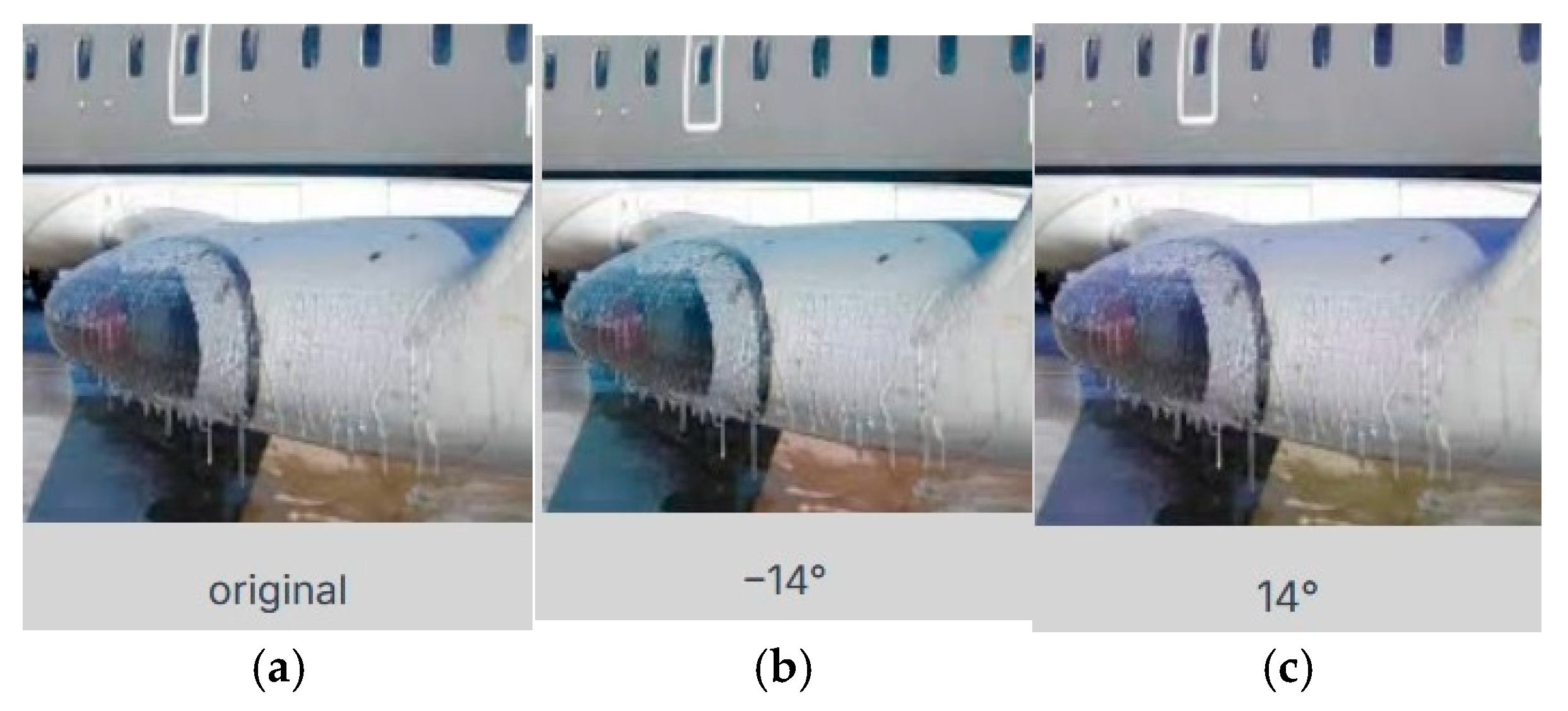
In the Hue Plus Minus process, additional hues were applied to the images. Example images from this process are shown in Figure 3.

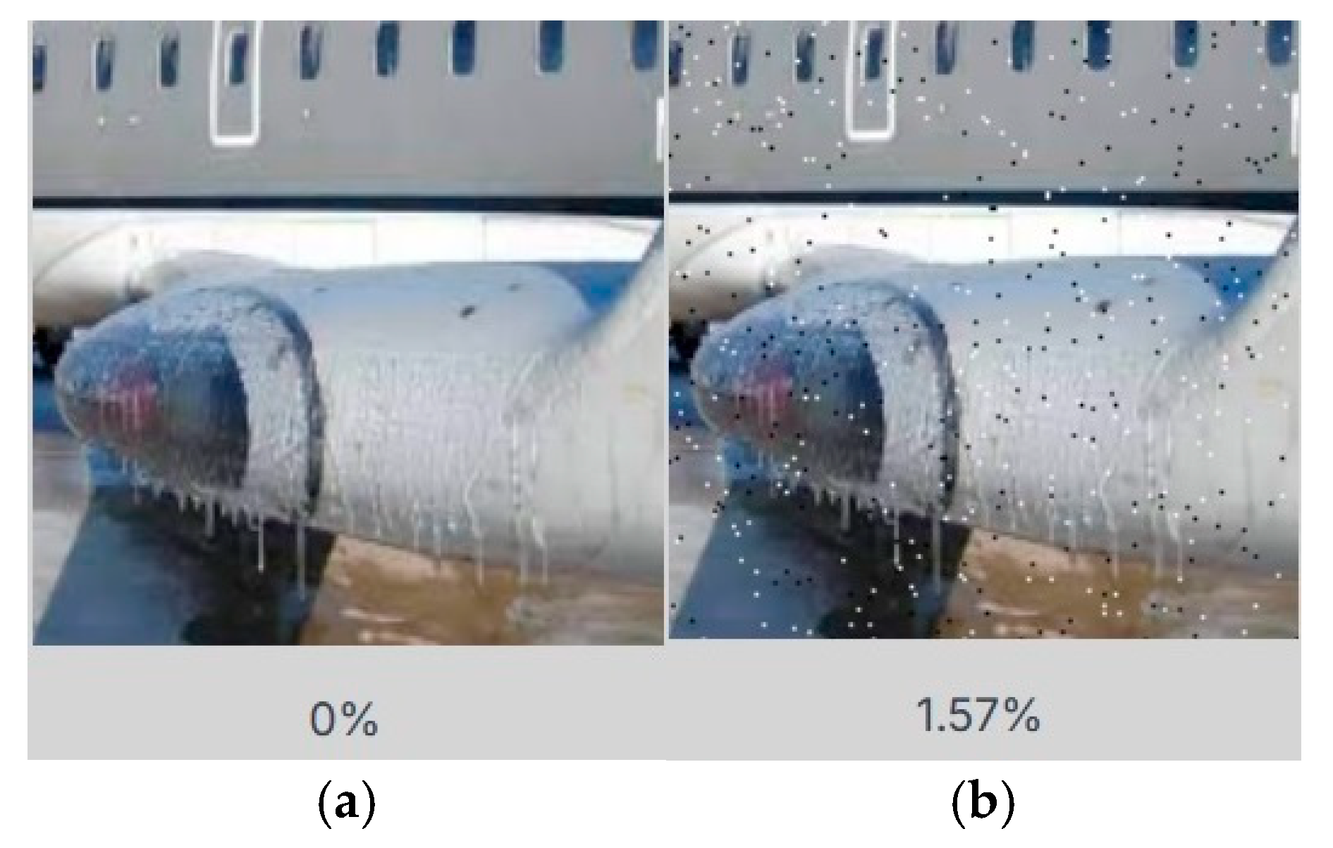
In the Noise process, noise was added to the images. The noise parameter was set to 10%. Example images are shown in Figure 4.

In this way, the main set of images was increased from 300 to 520 photos. The dataset was balanced to reflect various environmental conditions. According to literature analysis, a balanced dataset allows for better object detection results [34]. Literature sources indicate that the minimum number of images required for reliable AI model training is approximately 200. Therefore, the number 520 was considered sufficient. Labels were added to each image in the final dataset. For this purpose, the Roboflow Universe platform was used. All labels were added manually. Although ice and snow are distinct phenomena, this study employs a single class due to their visual similarity and frequent co-occurrence (e.g., snow layers over ice). However, this design limits the method’s effectiveness to scenarios where both appear simultaneously. When only one phenomenon occurs, the system cannot differentiate threat levels between dry snow, wet snow, or ice—a critical constraint for operational deployment.

After the labeling process was completed, the dataset was divided into three subsets: a Train set with 480 images, Validation set with 20 images, and Test set with 20 images. Additionally, all images were converted to a size of 640 × 640 pixels. In this way, a ready-to-use dataset was created, enabling the AI model training process to be carried out.

3.1. The Process of Training, Testing, and Validating Models

Taking technological capabilities into account, it was decided to conduct two AI model training processes: an automatic process and a manual process. The first was carried out using the Roboflow training platform. The second was performed manually using custom code and the Google Colab computational environment.

3.1.1. Automatic Training Process

The YOLOv8 (Ultralytics) framework is an advanced, stable model for object detection, segmentation, and classification, utilizing a CNN architecture with anchor-free detection and C2f modules for high precision and speed. The framework is available in variants from yolov8n (nano) to yolov8x (extra-large), and this project used yolov8s to balance performance and speed. Implemented in Python 3.9 with PyTorch v.2.6.0 and Roboflow cloud servers, YOLOv8 automatically localized and classified snow/ice on aircraft in images. Training was conducted on the Roboflow platform v.2025 in Accurate mode, ensuring a high detection precision. Roboflow’s automated environment streamlined data preparation and parameter optimization. The training process was fully automated, with Roboflow dynamically adjusting key hyperparameters (epochs, batch size, learning rate) based on data characteristics and training mode. Training lasted 45 min and 18 s, influenced by model architecture and computational resources. Post-training, Roboflow generated a detailed report, evaluating the model using metrics like mean Average Precision (mAP) and mAP@50:95. The evolution of these metrics is illustrated in Figure 5.

The detection performance graph for the automated model can be divided into four phases:

• Early phase (0–40 epochs): Unstable values with sharp fluctuations in mAP;
• Intermediate phase (40–120 epochs): Gradual increase in mAP from ~0.15 to 0.25, accompanied by pronounced oscillations;
• Advanced phase (120–200 epochs): Stabilization of mAP within the 0.2–0.25 range;
• Final phase (>200 epochs): Systematic rise to ~0.3, indicating progressive model generalization.

The parallel, more gradual increase in mAP@50:95 (lighter line), reaching values around 0.15 in the final training phase, indicates a robust detection quality across varying IoU thresholds. The Box Loss graph, illustrating changes in the bounding box localization loss function over successive training epochs, has been shown in Figure 6.

The observed learning process exhibited the following characteristic phases:

• Initial phase (0–20 epochs): Sharp increase to a maximum value of ~4.1, followed by a rapid decline to ~3.0;
• Stabilization phase (20–80 epochs): Values oscillated within the 2.5–3.0 range, with visible fluctuations;
• Maturity phase (80–200 epochs): Relatively stable level around 2.5–2.7, showing a slight downward trend;
• Final phase (200–218 epochs): Slight increase followed by a decline, suggesting the attainment of a local minimum.

Stabilization of Box Loss at approximately 2.5 indicates the model’s effective learning of geometric parameter determination for regions of interest, which is critical for precise localization of ice–snow deposits on aircraft surfaces. An Object Loss graph, illustrating changes in the loss function related to object detection, is shown in Figure 7.

Figure 7 consists of three main phases:

• Initial phase: Sharp increase to approximately 7.5, followed by a rapid decline.
• Intermediate phase (20–150 epochs): Stabilization at a level of 3.0–3.5.
• Final phase: Slight increase and eventual stabilization at approximately 3.5.

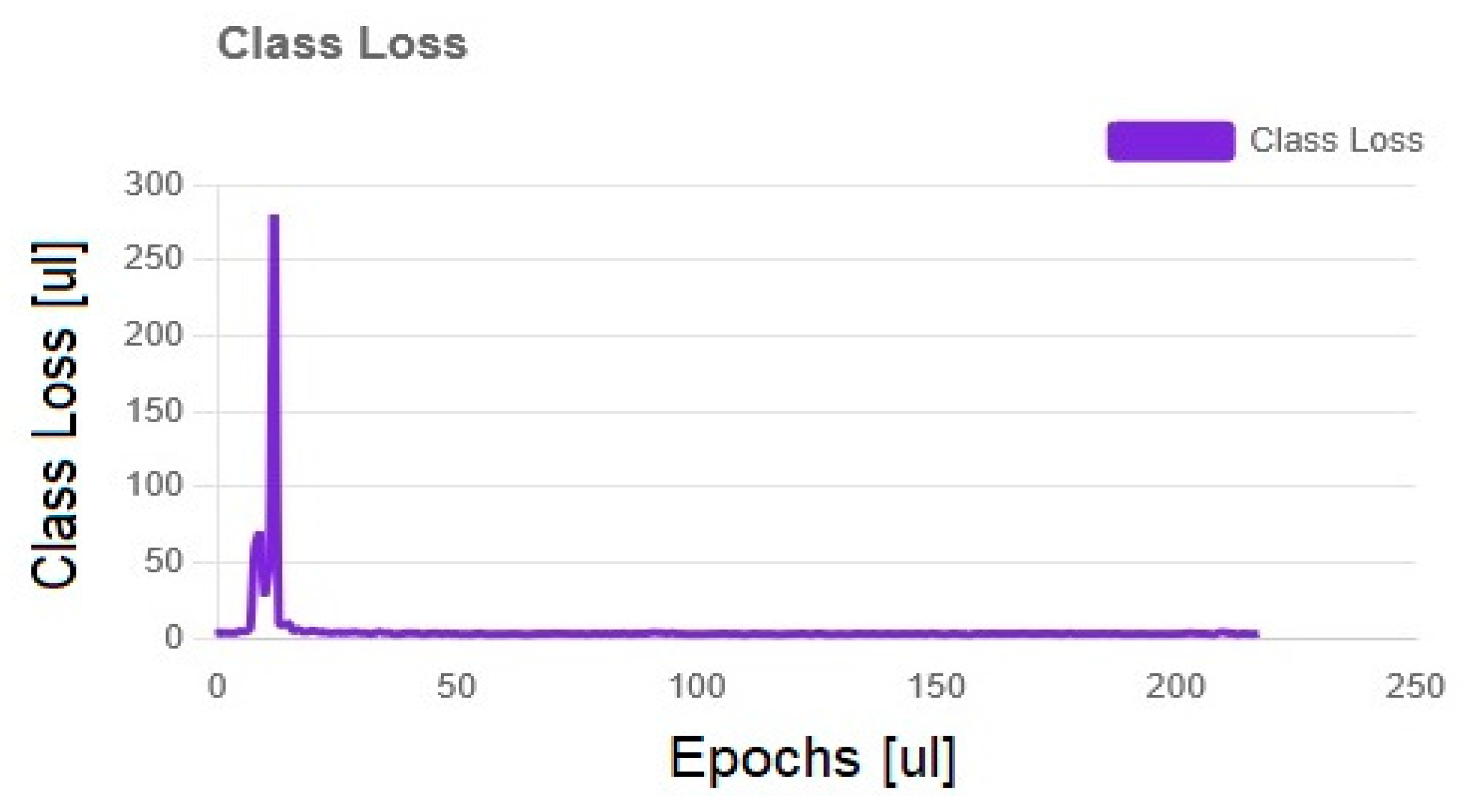
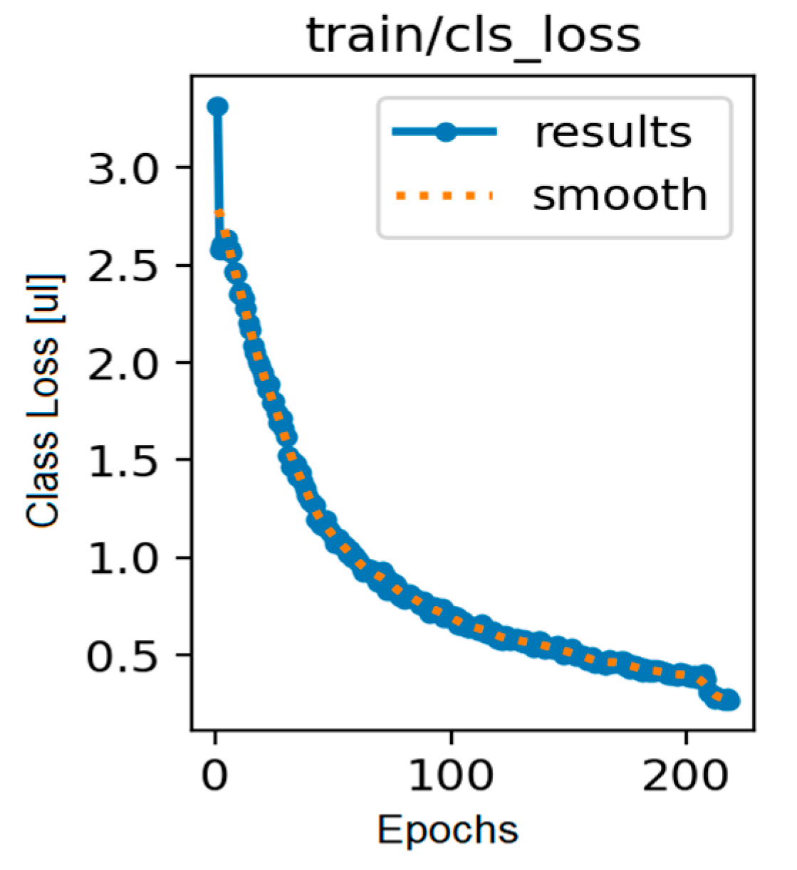
Stabilization of Object Loss indicates that the model has reached an optimal equilibrium between detecting true objects and generating false positives. The Class Loss graph, shown in Figure 8, illustrates the process of classification error minimization.

In the initial phase of the graph, a sharp initial spike is visible. An extremely high value of around 270 occurs near the 10th epoch. This is followed by rapid convergence: a drastic drop to below 10 by the 20th epoch. From this point on, long-term stabilization occurs: from around the 25th epoch, the value remains close to zero. When using a single class, class loss is not significant and does not affect the assessment of the model’s effectiveness. In such a case, class loss does not provide meaningful information about the model’s performance, as there is no possibility of confusion between classes. The above results were calculated on a separate test set, ensuring an objective evaluation of the model’s generalization capabilities.

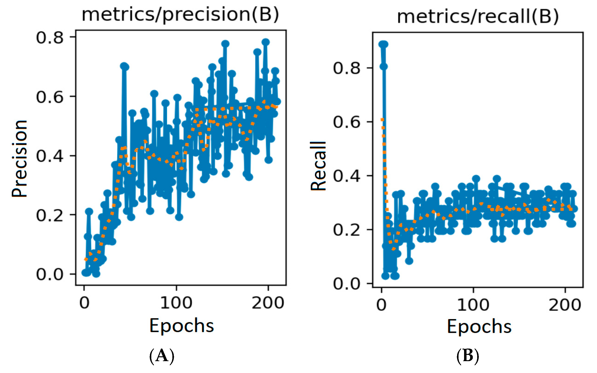
In the research process, charts showing changes in precision and recall as a function of the number of epochs were used. The resulting metrics enabled verification of the model’s quality, as they allowed monitoring of how effectively the model minimized the number of false alarms during the training process. The precision and recall curves are shown in Figure 9.

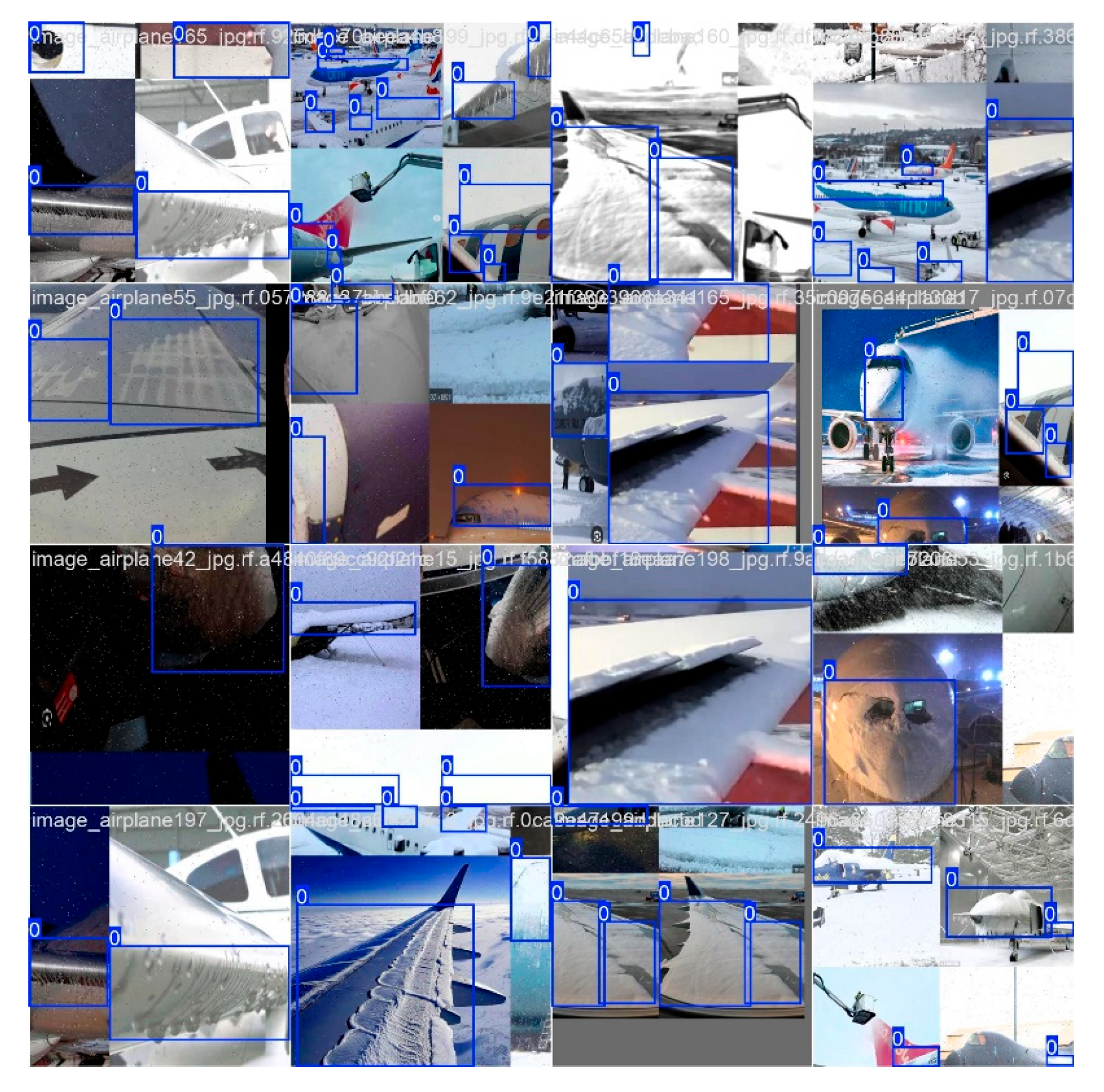
For the given values of precision and recall, the calculated F1 score was 0.32. Additionally, Roboflow enabled the visualization of results on sample validation images and the determination of the model’s performance. Example images from the validation process are shown in Figure 10.

This approach ensures the repeatability of the experiment and enables an objective comparison of the obtained results with other solutions available in the literature.

3.1.2. Manual Training Process

The same dataset as in the automatic process was used for AI model training. The training process was carried out in the Google Colab Pro environment with T4-NVIDIA CUDA GPU hardware acceleration (NVIDIA, Santa Clara, CA, USA). For manual training, 218 epochs were used—the same number as in the automated training, in order to compare the models. Data loading and preprocessing included scaling images to a size of 640 × 640 pixels. The most important hyperparameters used for model training are presented in

Table 1. A summary of the key hyperparameters and their values used for model training.

Hyperparameter Name	Value	Description
Batch size	16	Number of samples processed simultaneously in one training iteration Data.
Number of epochs	218	Number of full passes through the training dataset.
Image size	640	Input image resolution used during training.
Optimizer	AdamW (lr = 0.002)	Algorithm for updating model weights, here AdamW with lr = 0.002.
Momentum	0.9	Momentum factor used in the optimizer to accelerate convergence.
Loss function	box, cls, dfl loss	Losses for object detection: localization, classification, DFL.
Weight decay	0.0005	Regularization parameter to prevent overfitting.

.

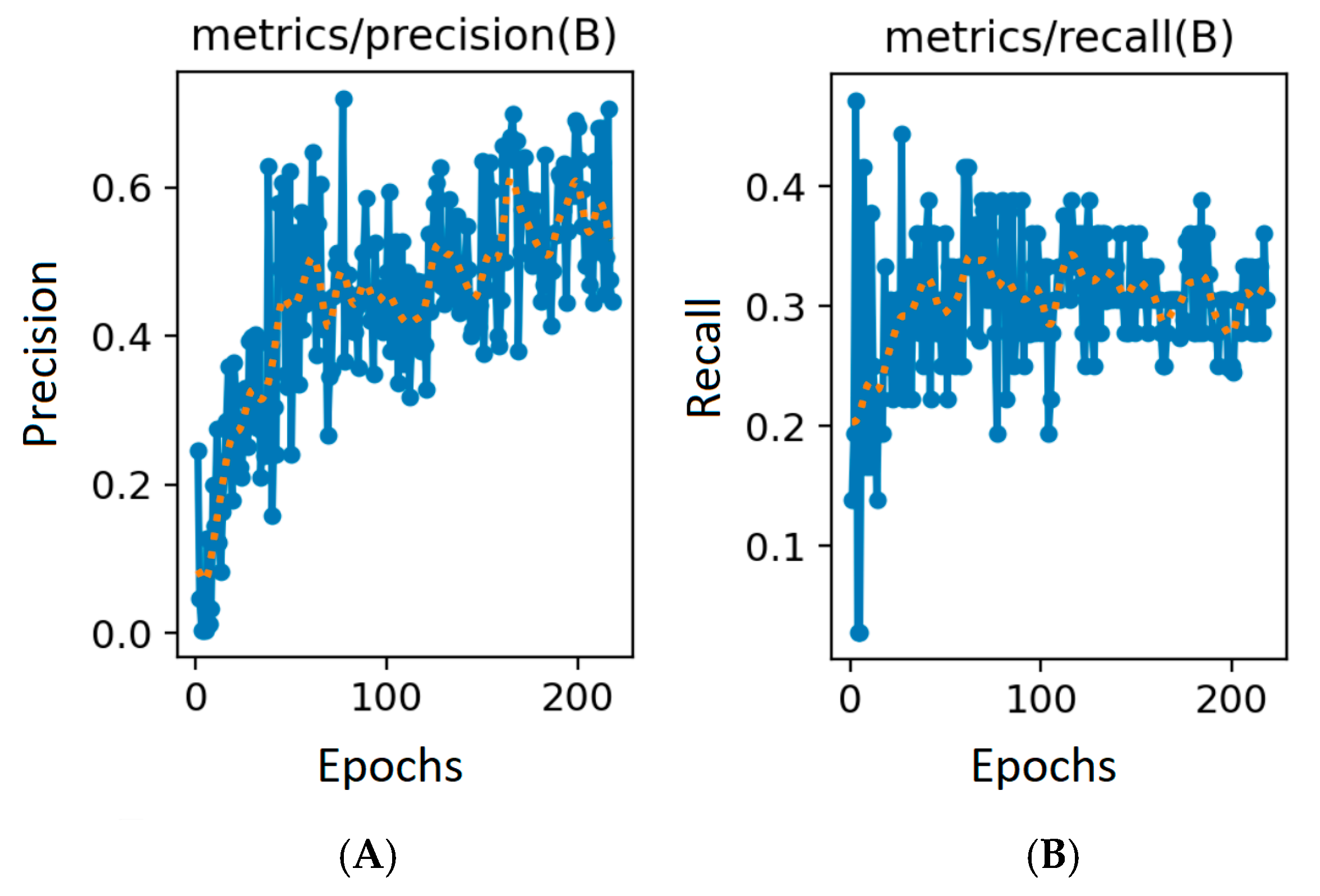
The model training process was conducted manually in the Google Colab environment, based on selected hyperparameters. The analysis included key aspects of the training process, convergence, and model quality. In this way, performance metrics for the manually trained model were obtained. Figure 11 presents the quality metrics (precision, recall, mAP50, mAP50-95).

Quality metrics exhibit the following characteristics:

• Precision: Increases from ~0.1 to 0.3–0.6, with noticeable fluctuations. This indicates the model is generating fewer false positives over time, though some instability persists;
• Recall: Rises from ~0.1 to 0.3–0.4, with variability similar to precision. The model becomes progressively better at detecting true snow and ice instances;
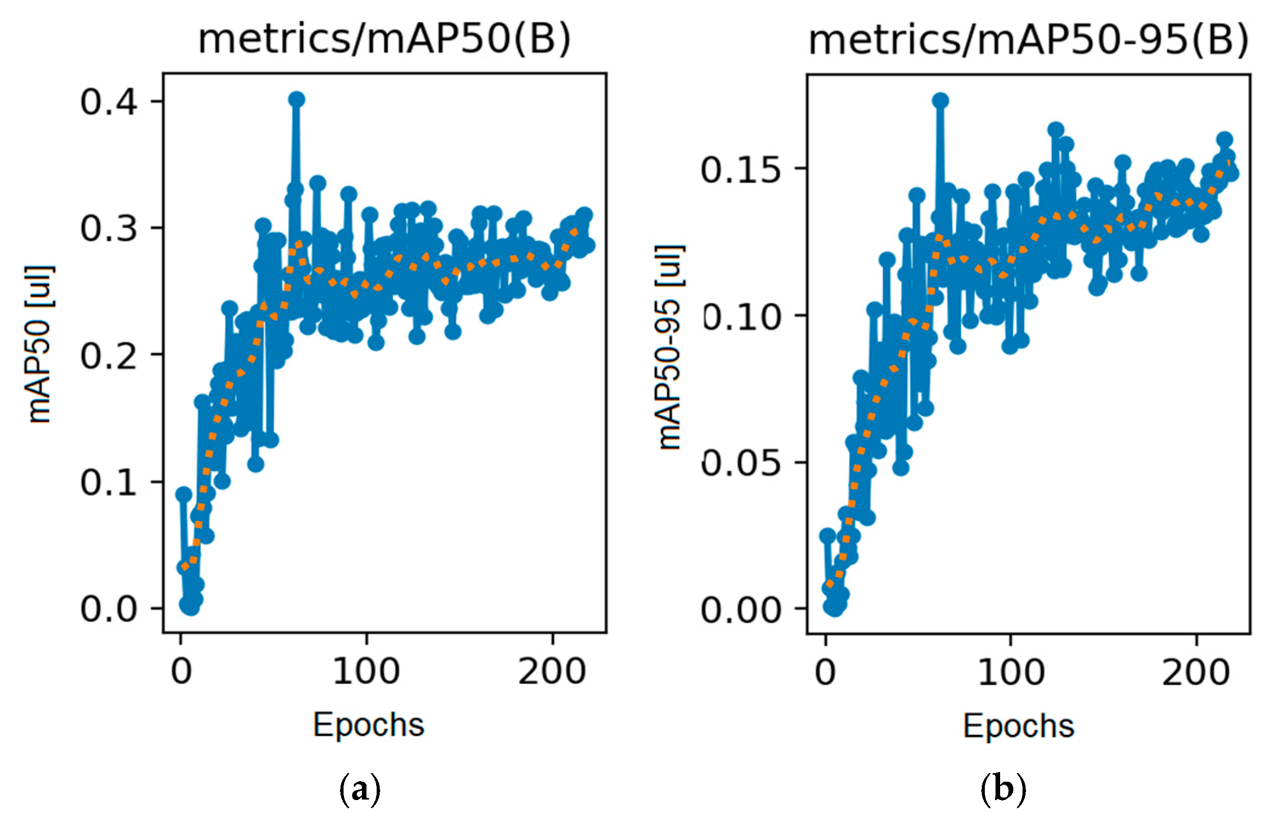
• mAP50: Mean average precision at an IoU threshold of 0.5 gradually improves to ~0.3, reflecting enhanced detection accuracy;
• mAP50-95: This more rigorous measure of precision across IoU thresholds (0.5–0.95) increases to ~0.15. It demonstrates moderate but steadily improving detection quality, even for stricter localization tasks.

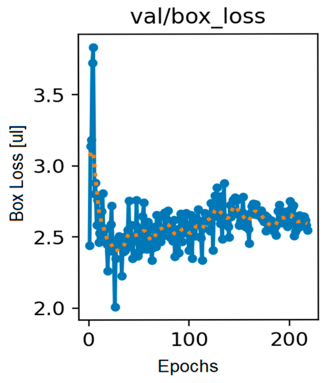
Figure 12 shows the progression of the Box Loss metric during training.

The box loss curves for the training and validation sets reveal how the model learns to precisely localize objects (snow and ice) in images:

• Training: Box loss systematically decreases from above 2.0 to below 0.5 over 218 epochs, indicating effective adaptation to the training data. The smooth curve suggests stable learning without abrupt parameter shifts;
• Validation: An initial sharp spike (reaching ~4.0) is observed, followed by rapid stabilization within the 2.3–2.7 range. The consistent validation loss level demonstrates that the model avoids overfitting and maintains generalization capabilities.

Figure 13 shows the progression of the Class Loss metric.

Class Loss reflects the model’s ability to correctly classify detected objects:

• Training: Class Loss drops sharply from ~3.5 to below 0.5, indicating rapid learning of class-discriminative features;
• Validation: An initial spike (up to ~30) occurs in early epochs, but values quickly drop and stabilize near training levels (~2–4). This dynamic suggests the model initially struggled to distinguish classes on the validation data but adapted swiftly.

Figure 14 shows the progression of the Distribution Focal Loss metric.

The DFL (Distribution Focal Loss) process involves determining the accuracy of bounding box localization predictions during training and validation. During training, a clear, systematic decline from values above 2.0 to below 0.5 was observed, indicating progressively improving localization precision (Figure 13). In validation, an initial peak (up to ~epoch 9) followed by rapid stabilization in the 3–4 range was noted, consistent with trends for box_loss and cls_loss.

A gradual improvement in object localization precision (decrease in dfl_loss) was observed in the DFL charts, which is a key indicator for object detection models, especially in applications requiring precise marking of icing areas on aircraft.

In order to evaluate the effectiveness of the model, the values of precision and recall on the validation set were recorded after each training epoch. Based on these results, charts were created showing changes in precision and recall as a function of the number of epochs. The charts are presented in Figure 15.

For the given values of precision and recall, the calculated F1 score was 0.33.

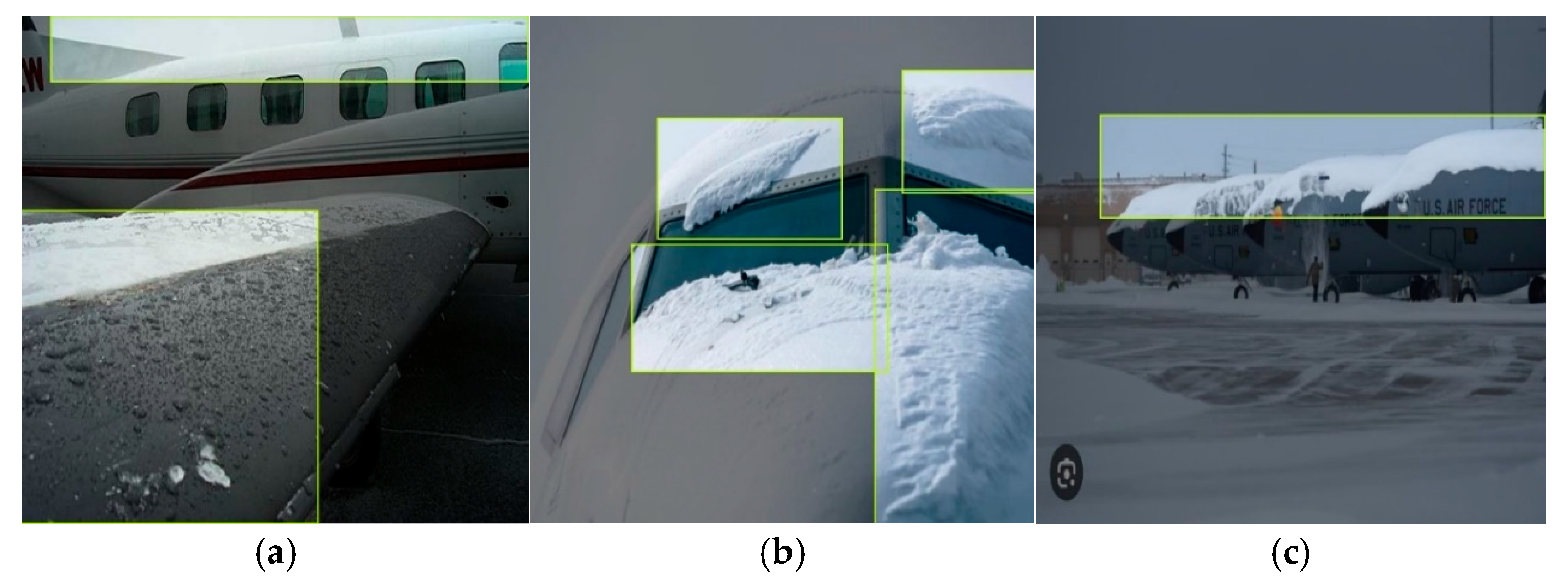
Figure 16 shows sample images from the validation process performed in manual mode.

The manual learning process in Colab proceeded stably: all key losses (box, class, dfl) on the training set show a systematic decrease without signs of overfitting. On the validation set, initial loss peaks are visible, but the model quickly stabilizes, indicating proper generalization. The quality metrics (precision, recall, mAP) show an increasing trend, although with greater variability than in automatic systems, which may result from manual hyperparameter selection and less process automation. The model achieves final mAP50 values of approximately 0.3 and an mAP50-95 of approximately 0.15, comparable to the results obtained in the automatic process.

The model was trained on 218 epochs in 0.592 h, which indicates a relatively efficient training process. The model architecture consists of 72 layers and contains 11,125,971 parameters, operating with an efficiency of 28.4 GFLOP. The training was conducted on a Tesla T4 graphics card (15,095 MiB of memory).

4. Discussion

After completing the learning processes and obtaining metrics for both models, the research results were compiled for comparison.

Box Loss Metric for the automatic method (YOLO): Starts with a clear jump to values around 4.0, then stabilizes in the range of 2.5–3.0 for most of the learning process. Significant fluctuations are visible, which do not decrease as learning progresses.

Box Loss Metric for the manual method (Colab): Shows a systematic decrease from 2.0 to below 0.5 for training data, which indicates better convergence. On the validation set, values stabilize around 2.4–2.5, similar to the automatic method.

Performance metric (mAP, mAP50-95) for the automatic method: The mAP chart shows very high variability with clear oscillations (0.1–0.3), with a general upward trend finally reaching about 0.3. The mAP@50:95 metric increases more steadily to a value of about 0.15.

Performance metric (mAP, mAP50-95) for the manual method: Achieves similar final values (mAP50 ≈ 0.25–0.3, mAP50-95 ≈ 0.15), but with smaller fluctuations. A more predictable learning curve with a clearer upward trend is also visible.

Object Loss Metric for the automatic method: Object Loss quickly stabilizes at 3.0–3.5 after an initial jump to 7.5. No clear downward trend was visible in later epochs.

CLS Loss and DFL Loss Metrics for the manual method: Both cls_loss and dfl_loss show a consistent decrease throughout the learning process. The smoothed curve indicates a more predictable optimization process.

Despite differences in the learning process, both methods achieve similar final values for key quality metrics. For mAP (mAP50), both the automatic and manual methods achieve values of around 0.25–0.3 in the final epochs, with a slight upward trend. Similarly, for mAP@50:95 (mAP50-95), both methods stabilize at around 0.15. It is worth noting, however, that in the manual method, these values are achieved with significantly lower training losses, which may suggest better model generalization and less risk of overfitting. The study implemented two different classification methods, both achieving comparable F1 scores of approximately 0.32 and 0.33, demonstrating equivalent effectiveness of both approaches in the analyzed task.

The values for obtained quality metrics such as mAP50 (0.25–0.3) and mAP50-95 (~0.15) may seem low from a theoretical point of view, but they are fully sufficient for practical application in a system cooperating with a camera mounted on a drone. The model does not analyze single, static images, but processes a video stream in which the camera records 30 frames per second. Even if the AI model recognizes an object only every third frame, the object will be detected in about 100 ms. In the case of better cameras that record 60 frames per second and allow analysis of every second frame, this time can be reduced to about 33 ms. This means that the object detection signal is generated at a high frequency, which is fully sufficient to trigger appropriate procedures, such as activating a trigger in the software. In practice, thanks to continuous video stream analysis and a high sampling frequency, the system minimizes the risk of missing a threat, thus ensuring sufficient reliability and effectiveness in applications related to aviation safety.

5. Conclusions

The automatic method, utilizing the YOLO architecture, was characterized primarily by a high configuration speed, as it requires minimal manual intervention in hyperparameter selection. This solution is optimized for computational efficiency, enabling rapid deployment and effective operation, which is crucial in real-time processing applications. There is little control over parameter settings during model preparation. In the context of atmospheric phenomena classification, a single detection class for ice and snow was used due to their frequent co-occurrence and visual similarity, which enables rapid hazard identification. However, this approach does not allow for distinguishing between different water phases (e.g., dry or wet snow) and requires additional validation when implemented in flight safety systems, representing a compromise between detection speed and precision. Additionally, higher fluctuations in loss functions such as Box Loss or Object Loss observed in the charts may help avoid becoming stuck in local minima, which can be beneficial when working with complex datasets. The automatic method also allows less advanced users to develop a model. In contrast, the manual method, implemented in the Google Colab environment, enabled better convergence, as evidenced by a systematic and smooth decrease in training losses to lower final values. The training process was more stable, and fluctuations in performance metrics such as precision, recall, or mAP were smaller compared to the automatic method. A significant advantage of the manual approach is the ability to precisely control and adjust parameters during training, allowing for better responses to specific challenges encountered when working with data. The choice of the appropriate method should depend on the specifics of the project. The automatic method (YOLO) is best when rapid model deployment is essential, expert resources are limited, real-time operation is required, and the training data is high quality and well describes real cases. The manual method is more appropriate when maximum model precision is required, which is crucial in the case of aircraft icing detection. Manual model training is particularly justified in situations where there are specific requirements regarding error characteristics, such as the need to minimize false alarms. This approach is also effective when expert knowledge is used for advanced model parameter tuning, and when working with heterogeneous data that requires an individual approach and flexibility in the modeling process.

The difference in precision is primarily due to the advanced, automated optimization and standardization procedures available in Roboflow, which are difficult to manually replicate in Google Colab without significant experience and knowledge of model optimization. Both methods achieve similar final results; however, the manual method provides better control over the training process, lower final loss values, and shorter model training time. In the context of detecting ice and snow on aircraft, where safety is paramount, the manual method is recommended, especially when expert resources are available. In aircraft ice detection, it is important not only to detect the presence of ice but also to precisely determine its location. To obtain more reliable and useful results, it is advisable to increase the number of photographs and conduct further research on the models. It is recommended to divide the detection process into classes corresponding to specific parts of the aircraft, such as wings, fuselage, engines, or propellers. Such studies will be carried out by the author in the future.