A Novel Energy Control Digital Twin System with a Resource-Aware Optimal Forecasting Model Selection Scheme

Abstract

As global energy demand intensifies across industrial, commercial, and residential domains, efficient and accurate energy management and control become crucial. Energy Digital Twins (EDTs), leveraging sensor measurement data and precise time-series forecasting models, offer promising monitoring, prediction, and optimization solutions for such services. Edge computing enables EDTs to deliver real-time management services placed closer to users. However, the existing energy management methodologies may fail to consider the limited resources of edge environments, which may cause service delays and reduced accuracy in management services. To solve this problem, we propose a novel energy control digital twin system with a resource-aware optimal forecasting mode selection scheme. The system dynamically selects optimal forecasting models by integrating statistical features of the input time series with available resources. It employs a two-stage approach: first, it identifies promising models through similarity detection in past time series; second, this initial recommendation is refined by considering the available computing resources to pinpoint the optimal forecasting model. This mechanism enhances adaptability and responsiveness in resource-constrained environments. Utilizing real-world LPG consumption data from 887 sensors, the proposed system achieves forecasting accuracy comparable to previous methods while reducing latency by up to 19 times in low-resource settings.

1. Introduction

As global energy demand intensifies across industrial, commercial, and residential domains, achieving accurate and efficient energy management has become a critical priority [1,2]. In response, Energy Digital Twins (EDTs) have emerged as promising tools for real-time monitoring and control of energy systems, offering data-driven monitoring, prediction, and optimization insights through virtual replicas of physical infrastructures [3,4,5]. These systems rely on time-series forecasting models to predict energy usage, demand/supply, sensor operation monitoring, malfunction detection, and the optimization of energy control operations [6]. However, the effectiveness of EDTs depends not only on the accuracy of forecasting models but also on their ability to operate within resource-constrained computing environments [7].

Modern time-series forecasting models span a wide range of complexity—from lightweight statistical approaches such as ARIMA and Prophet to computationally heavy deep-learning-based models such as the CNN, LSTM, GRU, and Transformer [8,9,10,11]. While advanced models often achieve higher accuracy, they typically require substantial computational resources and longer inference times, which are problematic in edge computing environments [12]. Edge computing, which processes data near the source to minimize latency and bandwidth, is particularly relevant in energy systems where immediate forecasting and control are crucial. On the other hand, deploying complex models across diverse edge devices with limited CPU and memory availability introduces a trade-off between accuracy and responsiveness [13]. Consequently, selecting the appropriate forecasting model in resource-constrained environments becomes essential.

The previous methods proposed diverse model selection schemes for accurate and efficient time-series services [14,15,16,17,18,19,20,21]. Some of the traditional methods are exhaustive search methods, which evaluate all candidate models to identify the optimal one, achieving high selection accuracy. AutoML platforms, such as AutoGluon and AutoKeras, automate the model selection process and reduce human intervention by leveraging hyperparameter optimization and architecture search. The automated solutions can identify the best-performing models. Other approaches include meta-learning-based model selection methods that train a meta-learner with the characteristics of time series, such as the length, skewness, kurtosis, seasonality, and trend, for adaptability and generalization on new tasks.

However, these methods assume abundant computational resources, which makes them difficult to simultaneously achieve both service responsiveness and high prediction accuracy. In real-world scenarios, particularly in edge-based energy management systems, concurrent requests from multiple energy control service users need to be handled. When computational resources are disproportionately allocated—either favoring high-complexity models or spreading too thin across many low-resource tasks—this can result in load imbalance, degraded prediction performance, and increased service response times. Furthermore, dynamic fluctuations in available resources, caused by factors such as hardware limitations or concurrent processing demands, can disrupt initial predictions of system capacity, exacerbating resource contention and compromising both accuracy and responsiveness in time-sensitive energy forecasting services.

The main contributions of this paper are as follows:

• A two-stage model-selection scheme: (i) A decision-tree meta-learner trained on 22 statistical meta-features proposes a candidate forecasting model, and then (ii) a KNN-based similarity correction refines that choice, improving selection accuracy without exhaustive search.
• A configurable runtime fallback that replaces the meta-learner’s pick with a lower-complexity model whenever its predicted inference time exceeds the current CPU quota or concurrency budget, ensuring bounded latency on edge devices.
• Integration of data collection, meta-feature extraction, model profiling, and runtime scheduling into a unified energy digital-twin-based control system.
• Experiments on LPG consumption from 566 sensors over 370 days under Docker-enforced CPU quotas with up to 30 concurrent requests, demonstrating an RMSE gap of <0.03 versus exhaustive search while achieving up to 18× service-time speedup.
• We demonstrate practicality on contemporary hardware (13th-Gen Intel i7 CPU with Docker CPU quotas), confirming that our method can be deployed on real-world edge platforms with strict latency and resource constraints.

The rest of this work is structured as follows. Section 2 reviews the related literature on time-series model selection and resource-aware energy management. Section 3 details the proposed framework, including data processing, model training, and meta-feature generation. Section 4 presents the experimental scenarios and evaluates the system’s performance. Finally, Section 5 concludes the paper and outlines future research directions for expanding the system to broader energy domains.

2. Related Works

The main purpose of this work is to select an optimal time-series forecasting model that meets user requirements by balancing model performance and execution time, while considering available computing resources. To establish an effective model selection framework for this purpose, it is crucial to understand the characteristics and limitations of existing approaches in time series forecasting and energy management systems.

Previous research has explored diverse strategies for model selection, tracing its evolution from early rule-based systems to modern automated and meta-learning-based approaches. Collopy et al. [14] introduced a foundational rule-based approach that employed 99 predefined rules and 18 time-series features, focusing on trends, uncertainty, and characteristic patterns to guide model choice. Building upon these early methodologies, Prudêncio et al. [15] proposed a meta-learning approach for time-series forecasting, leveraging features such as length, skewness, and kurtosis to learn their relationship with model performance. Subsequently, automated platforms such as AutoGluon [16] and AutoKeras [17] were developed to streamline model selection through automated hyperparameter optimization and architecture search, reducing human intervention. More recent studies have further advanced meta-learning-based methodologies: Talkhi et al. [18] applied meta-learning to COVID-19 forecasting using ARIMA and TBATS models; Fischer et al. [19] integrated considerations of explainability, model complexity, performance, and carbon emissions; Yao et al. [20] enhanced selection accuracy through clustering and weighted representation learning; Kozielski et al. [21] introduced a decision-support system using stacking-based meta-learning for LPG consumption forecasting without distinguishing user types. Despite these advancements, most existing approaches primarily focus on optimizing prediction accuracy based on static data features while neglecting the critical trade-offs between model performance, execution time, and dynamic resource availability. This gap limits their applicability in real-time, resource-constrained environments such as edge-based energy management systems.

Table 1. Comparison of the existing methods and the proposal.

Category	Automation Level	Real-Time Latency	Resource Awareness
[14]	Manual rule based	X (Not supported)	X
[16,17]	Fully automated	X	X
[15,18,19,20]	Automated	△ (Partially supported)	X
[21]	Semi-automated	X	X
The proposed framework	Fully automated	O (Fully supported)	O

summarizes these existing model selection approaches side by side, highlighting each method’s strategy and its lack of resource awareness.

To overcome these limitations, this gap motivates our contributions. In response, this paper proposes a digital-twin-based efficient energy control framework that integrates meta-learning with resource-aware model selection. The system collects energy consumption data, extracts statistical features—including trends, seasonality, skewness, and kurtosis—to generate meta-features, and characterizes candidate models by their complexity, performance, and execution time. By combining these meta-features and model profiles, the proposed framework dynamically selects the optimal forecasting model that satisfies user requirements while adapting to available computing resources.

3. Proposed System

3.1. System Overview

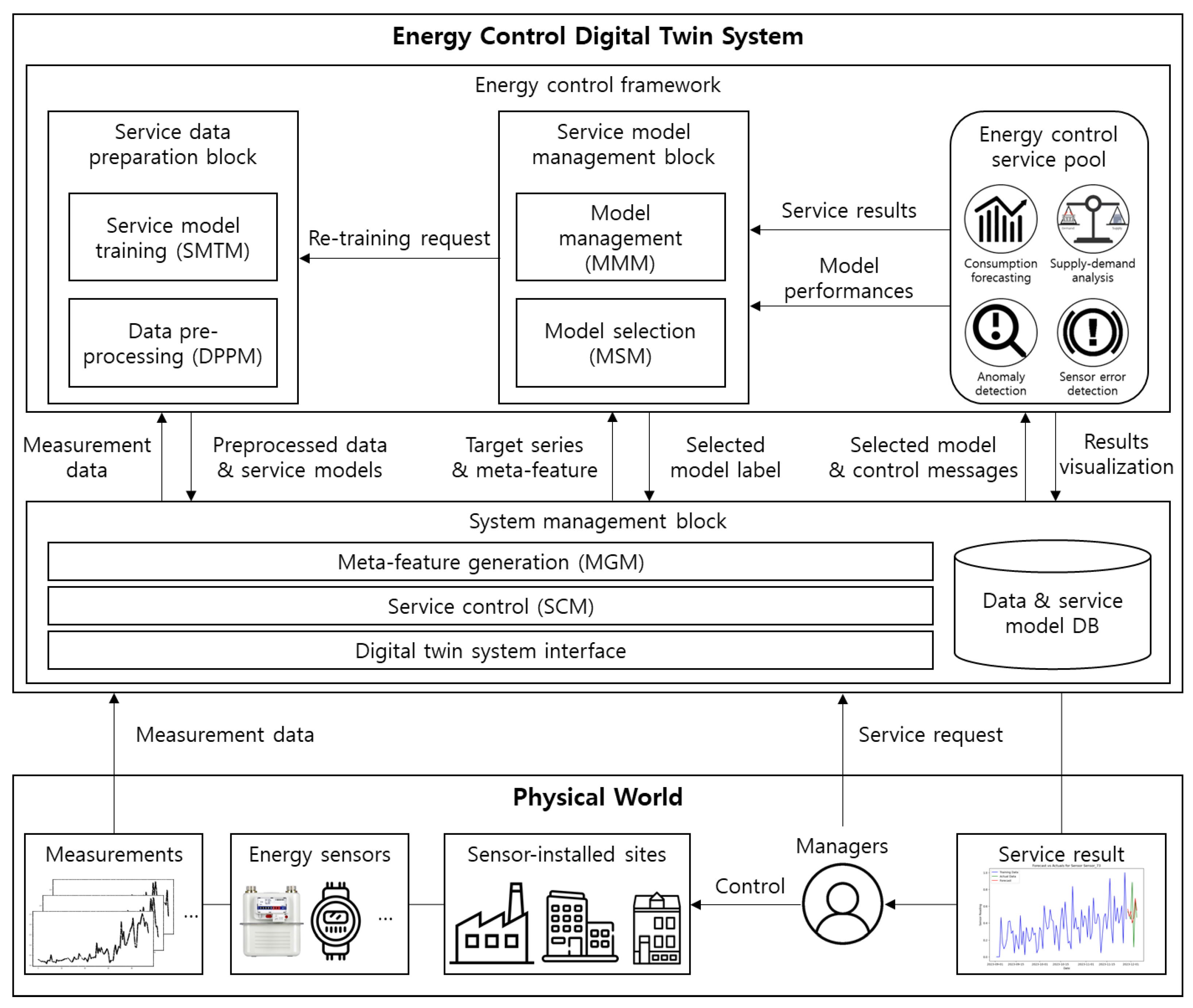
The overview of the proposed energy control digital twin system is illustrated in Figure 1. The figure shows the end-to-end workflow: from energy data collection, through the digital twin control system, to energy management services delivered to users. The figure consists of two parts: the physical world and the proposed energy control system. In the physical world where the energy sensors and sensor-installed sites exist, the energy sensors collect energy data such as energy usage, sensor state from sites such as factories, buildings, and offices, and they transfer the data to the near-edge server. The managers request the energy control service for the system, get service results, and optimally control the sites. The proposed system takes the measurement data and service requests as input. The system preprocesses raw measurements and stores them in the data repository. The service model is trained offline on these data. A meta-feature that can be used as the selection criterion to select the optimal service model is created with measurement data and the service model information. Our scheduler queries the OS for available CPU cores and current CPU quota usage and then selects the model whose worst-case inference time fits within the measured budget. Finally, the system visualizes the service results and updates the models based on feedback.

3.2. Definition of the Meta-Features

In this paper, we define the meta-feature vector as a 22-dimensional representation of each time series, consisting of both statistical characteristics and model-derived performance indicators, as summarized in

Table 2. The list of trained time-series forecasting models and their characteristics.

Model Name	Deep Leaning	Main Architecture	Key Features
TFT (Temporal Fusion Transformer)	●	Transformer + LSTM	Strong performance on complex time series
TF (Transformer)	●	Self-Attention	Requires positional encoding for time series
LSTM	●	Recurrent Neural Network	Used for learning long-term dependencies
DNN	●	Multilayer Perceptron	Contains multiple hidden layers
CNN	●	Convolutional Neural Network	Effective in local pattern detection
GRU	●	RNN variant	Lighter and faster than LSTN
RNN	●	Recurrent Neural Network	Used for processing sequential data

. The first set of features captures the statistical and structural properties of the series. These include basic distributional statistics such as the mean, variance, standard deviation, maximum value, skewness, and kurtosis, as well as complexity-related attributes such as entropy, linearity, nonlinearity, stationarity, spikiness, curvature, flat spot length, and the number of missing values. These features characterize the shape, consistency, and irregularities of the series over time. The second set of features captures the forecasting performance of six representative deep learning models—RNN, DNN, CNN, LSTM, GRU, and Transformer—as well as TFT. For each model, four standard error metrics (MAE, MSE, RMSE, and RMSLE) are computed by applying the pre-trained model to the corresponding time-series segment. Finally, we include the best model label, which indicates the forecasting model that yielded the lowest error across all candidates. This serves as the ground truth during meta-model training. Together, these 22 meta-features provide a rich representation of both the intrinsic characteristics of the time series and their forecasting behavior across diverse model architectures. The features are used as the selection criteria for the optimal service model.

These data can be classified as time-series data since the data are usually collected or recorded as successive and evenly spaced points in time. Since it is difficult to specify and capture the characteristics of the selection criteria with a single time-series datum or a single energy control service model, it is necessary to consider the different aspects of the data. Therefore, meta-features are generated with statistical features of the energy usage time-series data, such as the mean, variance, seasonality, etc. The details of the meta-features are described in Section 3.5.

3.3. Service Data Preparation Block

Data Preprocessing Module (DPPM)

In this data preprocessing module (DPPM), a specific process of preprocessing the energy usage measurement data is described. When a factory, office, or business site consumes energy, such as electricity or gas, energy measurement sensors, including an LPG meter and flow sensor, collect the energy usage at a consistent interval. For example, LPG (liquefied petroleum gas) measurement data can represent a certain amount of usage data from various sensor-installed sites. Sensor-installed sites refer to factories, houses, office buildings, etc. Since the data are collected from diverse places, the characteristics of the measured data are also different. For example, even though the sites use the same LPG energy, their usage varies over time. Therefore, it is necessary to preprocess the dataset to train the service models and extract the meta-features.

To preprocess the measurement data, the system queries data from a database for a certain period of energy usage data from various sites. Since the dataset contains different characteristics from site to site, it is necessary to process the data into the same range. For example, some sites are located in cold areas, which require people to use more energy for heating, while other sites in hot areas do not need to use the same amount of energy for heating. The energy consumption difference over a year among three different sites is represented in Figure 2. The figure shows the daily measurements of LPG usage in three distinctive places.

In case (a) of Figure 2, the data range is from 0 to higher than 600, which can be seen as an outlier or an anomaly value, while the data range in case (b) is only from 0 to 1, and case (c) contains multiple consecutive zero spots. The peak values of both cases show spiky patterns, high fluctuations, noises, and straight zeros, which could make it difficult for forecasting models to capture the trend and seasonality of the data, generalize to unknown patterns, and increase the model training time. Therefore, it is important to standardize the various data into a common range to ensure the stability and performance of the models. The preprocessing procedure is depicted in Algorithm 1, and the dataset that we used to preprocess is introduced in Section 4.

Algorithm 1 is Preprocessing procedure for data cleaning and interpolation.

Algorithm 1 Data Cleaning and Outlier Handling

1: Input: Raw dataset D from $csv$ 2: Output: Cleaned dataset $D_{final}$ saved as ${csv}_{final}$ 3: procedure REMOVEUNINFORMATIVECOLUMNS(D) 4:            for each column c in D (excluding first column) do 5:                    if all values in c are 0 then 6:                              Mark c for removal 7:                    else 8:                              Compute longest run of consecutive zeros in c 9:                              if maximum consecutive $zeros>60 days$ then 10:                                    Mark c for removal 11:                              end if 12:                  end if 13:              end for 14:              Remove marked columns from D 15:              return $D_{cleaned}$ 16: end procedure 17: $D_{cleaned}$ ← REMOVEUNINFORMATIVECOLUMNS (D) 18: procedure REPLACEOUTLIERSWITHZSCORE(D) 19:      for each column c in D (excluding first) do 20:            Compute mean μ and std. deviation σ of c 21:            for each value $x_i$ in c do 22:                  Compute $z_i={\displaystyle \frac{x_i-\mu }{\sigma }}$ 23:                  if ${|z}_i|\ge 3$ then 24:                          Replace $x_i$ with $x_{i - 1}$ if $i>0$, else with μ 25:                  end if 26:            end for 27:      end for 28: end procedure 29: $D_{final}$ ← REPLACEOUTLIERSWITHZSCORE ($D_{cleaned}$)

After removing consecutive zeroes, we applied interpolation using the z-score. The z-score is a statistical measurement that shows how far a specific data point is from the mean value in terms of standard deviations. This score can be used to detect outliers, and its formula is as shown in Equation (1):

$$\mathrm{z}={\displaystyle \frac{x-\mu }{\sigma }}$$

(1)

where $x$ is the data point, $\mu$ is the mean of the time-series data, and $\sigma$ represents the standard deviation of the time series. Since the time series contains outlier values, as shown in Figure 2a, the values need to be interpolated. Then, the value is replaced by its previous day’s measurement value. This is because even though the value $x_i$ is interpolated into the average of $x_{i-1}$ and $x_{i+1}$, it is still high enough to be seen as an outlier where only the observed value is too high. Finally, when the data cleaning is over, the preprocessed dataset is stored in the database and used by the Service Model Training Module.

3.4. Service Model Training Module (SMTM)

In the Service Model Training Module (SMTM), a diverse range of time-series forecasting models are trained using preprocessed data. In this paper, we trained models ranging from traditional deep learning models, such as a CNN (convolution neural network), an RNN (recurrent neural network), and LSTM (Long short-term memory), to attention-based transformer models and GluonTS models, including TFT (Temporal Fusion Transformer), etc. [22]. A list of the trained models is given in Table 2. Each model is trained with the same training dataset to ensure fair selection among several candidates.

The proposed system does not include statistical time-series models, such as ARIMA (Auto-Regressive Integrated Moving Average) or Prophet. Even though the models are commonly used because they require relatively little training time or less training data than deep learning models, it is difficult for them to consider explicit variables, events, or categorical information, so these models need to be trained every time they are used. This can also cause low forecasting performance.

For the deep learning models, we applied a parameter tuning mechanism to ensure the forecasting performance of each model. The system offers various lengths of forecasting horizons, which refers to the future target days to predict, from 7 days to 30 days, with a 7-day interval. The deep learning models are trained and stored on the database, and their attributes, including the number of parameters, complexity, and execution time, are used to generate the meta-features.

3.5. System Management Block

Meta-Feature Generation (MGM)

This subsection presents the process of meta-feature generation. As introduced in Section 3.2, a meta-feature is a combination of the attributes of energy usage measurement time series. The attributes of the time series are based on statistical features such as the mean, variance, linearity, etc. Features such as kurtosis, skewness, entropy, spikiness, etc. were extracted since the time-series data that we would like to consider contain high nonlinearities and uncertainties, as depicted in Figure 2. A summary of the meta-features that we extract is given in

Table 3. The extracted meta-features and descriptions.

Number	Feature	Description
1	Mean	The average value of the time series
2	Variance	The variability of the time series
3	Standard deviation	The spread of the time series
4	Max value	The maximum value of the time series
5	Kurtosis	The peakedness or tail-heaviness of the time series
6	Skewness	The asymmetry of the time-series distribution
7	Entropy	A measure of the complexity or disorder in the frequency domain
8	Linearity	Degree to which the series follows a linear pattern
9	Stationarity	Degree to which statistical properties (mean, variance) remain constant over time
10	Missing values	The number of missing observations in time series
11	Spikiness	The severity of sudden sharp peaks in time series
12	Curvature	Degree of bending in the trend component
13	Flat spot length	Length of straight zeros in time series
14	Nonlinearity	Degree to which the time series deviates from a linear model
15	Performance metrics of RNN	Columns of the pre-trained RNN model for each series, including MAE, MSE, RMSE, RMLSE
16	Performance metrics of DNN	Columns of the pre-trained DNN model for each series, including MAE, MSE, RMSE, RMLSE
17	Performance metrics of CNN	Columns of the pre-trained CNN model for each series, including MAE, MSE, RMSE, RMLSE
18	Performance metrics of LSTM	Columns of the pre-trained LSTM model for each series, including MAE, MSE, RMSE, RMLSE
19	Performance metrics of GRU	Columns of the pre-trained GRU model for each series, including MAE, MSE, RMSE, RMLSE
20	Performance metrics of Transformer	Columns of the pre-trained Transformer model for each series, including MAE, MSE, RMSE, RMLSE
21	Performance metrics of TFT	Columns of the pre-trained TFT model for each series, including MAE, MSE, RMSE, RMLSE
22	Best model	The name of the most accurate forecasting model

.

In addition to statistical features extracted from the time-series data (e.g., mean, standard deviation, skewness, kurtosis, and entropy), the MGM module also includes model-specific performance meta-features. During the offline training phase, multiple forecasting models (e.g., LSTM, GRU, CNN, Transformer) were trained on each time series, and their prediction performance was measured using metrics such as the RMSE, MAE, MSE, and RMLSE. These performance scores were then included in the meta-feature set, providing the meta-learner with rich historical context about how different models behaved on similar types of data.

The model performance is measured using five metrics: the mean absolute error (MAE), mean squared error (MAE), root mean square error (RMSE) and root mean squared log error (RMSLE). These five metrics were used to measure the differences between the forecasting values and the real values. Since these metrics are errors, a smaller error means that the forecasting is more accurate. The formulas of the five metrics are as follows:

$$\mathrm{M}\mathrm{A}\mathrm{E}={\displaystyle \frac{1}{n}}\sum _{i=1}^n\left|y_i-{\widehat{y}}_i\right|$$

(2)

$$\mathrm{M}\mathrm{S}\mathrm{E}={\displaystyle \frac{1}{n}}\sum _{i=1}^n{(y_i-{\widehat{y}}_i)}^2$$

(3)

$$\mathrm{R}\mathrm{M}\mathrm{S}\mathrm{E}=\sqrt{{\displaystyle \frac{1}{n}}\sum _{i=1}^n{(y_i-{\widehat{y}}_i)}^2}$$

(4)

$$\mathrm{R}\mathrm{M}\mathrm{S}\mathrm{L}\mathrm{E}=\sqrt{{\displaystyle \frac{1}{n}}\sum _{i=1}^n{(\log \left(1+{\widehat{y}}_i\right)-\mathrm{l}\mathrm{o}\mathrm{g} (1+y_i\left)\right)}^2}$$

(5)

Furthermore, the dataset is labeled with the best-performing model for each time series according to multiple criteria (e.g., lowest RMSE or MAE). This annotation is used during the training of the meta-learner to establish a supervised learning objective. The inclusion of both statistical and performance-based meta-features allows the model selection process to be more informed, balancing data-driven characteristics with empirical forecasting behavior.

3.6. Service Model Management Block

3.6.1. Model Selection Module (MSM)

The model selection process begins with the extraction of statistical features from the incoming time series. For each sensor’s time-series data, a fixed-length meta-feature vector is computed, capturing distributional and structural characteristics such as the mean, standard deviation, variance, skewness, kurtosis, entropy, and stationarity. These features are used as inputs for both the decision-tree-based classifier and the similarity-based reasoning module in the subsequent selection stages.

To select the most suitable forecasting model under varying time-series characteristics and constrained computing environments, we propose a hybrid model selection strategy that integrates decision-tree-based classification with similarity-based reasoning. This strategy enables the system to make adaptive, accurate, and resource-aware model decisions in real time.

The primary prediction is generated by a decision tree classifier trained on statistical meta-features extracted from each sensor’s time series (e.g., mean, variance, skewness, entropy). The classifier outputs a candidate model $m_{DT}$ along with its associated confidence score ${conf}_{DT}$. Simultaneously, a similarity-based reasoning module retrieves historical data of similar time series using a K-Nearest Neighbors (KNN) approach. All 22 statistical meta-features listed in Table 3 are first standardized via z-score normalization. Each feature is centered to zero mean and scaled to unit variance. Then, the similarity is calculated with the following distance-weighted kNN rule:

$$\mathrm{d}\left(x,y\right)=\sqrt{\sum _{j=1}^{22}{(\widetilde{x_j}-\widetilde{y_j})}^2}$$

(6)

$$s\left(m\right)=\sum _{i=1}^k{\displaystyle \frac{1\left[m_i=m\right]}{1+d_i}}$$

(7)

where $x$ refers to the meta-feature vector of the target time series, $y$ stands for the previous meta-feature vector, and $j$ indicates the meta-feature index. $i$ is the index of the $i$-th neighbor among the $k$ nearest neighbors of $x$. $d_i$ is the distance between $x$ and the $i$-th neighbor, and $\mathrm{m}$ is a candidate forecasting model label. Based on the frequency and similarity-weighted performance of the models used for the nearest neighbors, a secondary prediction $m_{KNN}$ is produced with confidence ${conf}_{KNN}$.

To combine both prediction signals, we define the following confidence-weighted hybrid score:

$$\mathrm{s}\mathrm{c}\mathrm{o}\mathrm{r}\mathrm{e}\left(\mathrm{m}\right)=w_{DT}·{conf}_{DT}\left(\mathrm{m}\right)+w_{KNN}·{conf}_{KNN}(\mathrm{m})$$

(8)

where $w_{DT}$ and $w_{KNN}$ are empirically defined weights (e.g., 0.6 and 0.4, respectively). The model with the highest score is selected as the initial candidate $m_{hybrid}$.

Although this hybrid scoring strategy enables fast and accurate selection, it does not directly account for model complexity at this stage. Instead, complexity is considered in a separate substitution step that follows hybrid selection. Each forecasting model is associated with a normalized complexity score $C\left(m\right)\in \left[\mathrm{0,1}\right]$ based on empirical attributes such as the parameter count and runtime performance. After selecting $m_{hybrid}$, the system checks whether this model remains feasible with the currently available CPU resources.

This substitution logic ensures that even in severely resource-constrained scenarios, the system selects a model that satisfies execution constraints while minimizing the loss in forecasting accuracy. Specifically, if the complexity of the initially selected model $m_{hybrid}$ exceeds a threshold ${\tau }_C$, and the currently available CPU level $A_{CPU}$ falls below a predefined limit ${\tau }_{cpu}$, the system initiates a fallback mechanism. The mechanism selects a replacement model $m’$ from the candidate pool $\mathcal{M}$ that has a lower complexity and can be executed within reduced latency. Formally, the selection criterion is defined as follows:

$$\begin{gathered} \mathrm{I}\mathrm{f} C\left(m_{hybrid}\right)>{\tau }_C \mathrm{a}\mathrm{n}\mathrm{d} A_{CPU}<{\tau }_{cpu}, \mathrm{then} \\ \mathrm{select} m’=arg\underset{\mathit{m}’\in \mathcal{M}}{\min }\{\mathrm{C}(\mathrm{m}’)|T(m’,A_{CPU})<\alpha ·T(m_{hybrid},A_{CPU})\} \end{gathered}$$

(9)

where $C\left(m\right)$ denotes the normalized model complexity, $T(m,A_{CPU})$ represents the expected execution time of model mmm at the available CPU level $A_{CPU}$, and $\alpha$ is the time reduction factor (e.g., 0.8). Among the valid alternatives, the system selects the model with the lowest complexity. If no such model exists, the original $m_{hybrid}$ is retained. This design guarantees that latency-critical applications continue operating within acceptable time bounds, even under limited computational capacity.

Figure 3 illustrates a flowchart of the overall model selection process, from the meta-feature input to the final resource-aware decision output.

3.6.2. Model Management Module (MMM)

In this model management module (MMM), the base models for the model selection module are managed by getting the service results and performances from the energy control service. Since this is about time-series forecasting, the measurement data differ as time goes by and may contain different characteristics, such as their trend, seasonality, and stationarity. Forecasting models may not be able to represent the new patterns. Therefore, if the service performance is lower than 80%, the MMM sends a re-training request to the SMTM. In addition, for the changing characteristics of time-series data, it is important to re-train the base models after a certain period of time. For instance, the energy usage for heating may increase during the winter season in comparison with the summer season, so even though measurement data are accumulated, the patterns will be different or even unknown to the forecasting models. For this reason, re-training is essential to maintain the energy control service performance and meet user requirements.

4. Experiments and Analysis

In this section, a case study of energy control is described. It is mainly based on the prediction of LPG (liquefied petroleum gas) usage. The following subsections show the experimental setup, specifications, and experimental results with an analysis.

4.1. Edge Computing Configuration

The proposed framework was implemented on the authors’ laboratory edge server. The server was equipped with a 13th Gen Intel(R) Core(TM) i7-13700k CPU processor (Intel Corporation, Santa Clara, CA, USA) and 64 GB of memory. For the time-series forecasting model training, an NVIDIA GeForce RTX 4090 (NVIDIA Corporation, Santa Clara, CA, USA) with 24 GB of memory was used. The edge server created docker environments for each model run and allocated the available CPU resources to each docker container. In this paper, the computation overhead of container generation was not considered because it was negligible compared to the execution time of the time-series forecasting models.

The execution time of the models was measured in docker environments on Ubuntu 24.04 (Canonical Ltd., London, UK). CPU resources were allocated to the dockers at levels ranging from 1% to 100% by increasing 1% on each run.

4.2. Dataset Description

Through the MGM module in Section Meta-Feature Generation (MGM), meta-features were generated by calculating the features of the measurement data. This subsection demonstrates how the meta-features were generated with real sensor measurements.

The dataset used in this study consists of real-world LPG usage data collected from HD Energy and KT (Korea Telecom), covering a period of 370 days from 1 September 2023 to 5 September 2024. A total of 887 sensors were installed across diverse environments, including residential buildings, commercial offices, factories, and restaurants throughout South Korea. In the preprocessing stage, sensors containing all-zero values or severe outliers were removed, resulting in a refined dataset of 566 valid sensors. Each sensor’s time series was converted into a set of meta-features representing statistical and dynamic characteristics of the signal. The meta-features include statistical indicators such as the mean, variance, standard deviation, kurtosis, skewness, and entropy, as well as time-series-specific attributes such as linearity and stationarity, as detailed in Table 3.

These meta-features were used as inputs to the meta-learning framework proposed in this study. The meta-learning model was trained to predict the most suitable forecasting model for each sensor by analyzing its meta-features. The forecasting models were trained on the same preprocessed dataset using an 80-10-10 split for training, validation, and testing, respectively. The goal of the dataset preparation and meta-feature extraction process was to enable fast and adaptive model selection under computational constraints, thereby supporting efficient time-series forecasting across a large number of sensors.

4.3. Experimental Scenario

To evaluate the effectiveness of the proposed meta-learning-based model selection framework in an energy management context, we designed a series of experiments that reflect practical energy control service conditions—in particular, limited computing resources and the need for fast response times. The experiments aim to assess whether the framework can deliver accurate forecasting results within acceptable service latency, comprising both model selection and inference time.

The evaluation was conducted using the preprocessed LPG usage dataset, consisting of 566 sensors out of 887 sensors, as described in Section 3.3. The experiments were structured along two key dimensions: computing resource levels and the number of sensors served concurrently.

First, five levels of CPU availability were considered: 20%, 40%, 60%, 80%, and 100%. These levels simulate a range of computing environments, from highly constrained computing resources to fully available ones. The execution time of each forecasting model was pre-measured from 1% to 100% of the CPU level and used as part of the decision-making input for the meta-learner, enabling resource-aware model selection.

Second, the scalability of the proposed system was tested by varying the number of sensors requesting model selection and forecasting simultaneously. Two execution types were defined: (1) single-sensor execution, where one sensor can fully use the available computing resources, and (2) multi-sensor execution, where 10, 20, or 30 sensors concurrently trigger model selection and prediction while competing in the resource-limited environment.

For each combination of CPU level and sensor request size, the proposed framework selected forecasting models based on extracted meta-features and predicted trade-offs between execution cost and forecasting performance. The selected models were then applied to their respective sensor data for evaluation.

The following performance metrics were measured:

• Forecasting accuracy (measured using the RMSE);
• Model selection time;
• Inference time of the selected model;
• Total service time (sum of selection and inference times);
• Performance deviation from the globally optimal model selected via exhaustive search.

The results were compared against an exhaustive search baseline, which evaluated all candidate models to select the best one for each sensor without considering time or resource constraints. This comparison enables a holistic assessment of the proposed system’s ability to deliver fast and accurate forecasting services while adapting to real-world computing limitations.

4.4. Experimental Results and Analysis

This section describes the experimental results of the proposed meta-learning-based model selection framework, focusing on its effectiveness in selecting appropriate forecasting models for LPG usage in constrained computing environments. The experiments aim to assess whether the framework can provide accurate forecasting results while minimizing the overall service time, including both model selection and inference.

The experiments were conducted with five different levels of CPU availability (20%, 40%, 60%, 80%, and 100%) and with varying numbers of concurrent model requests (1, 10, 20, 40, 60, 80, and 100). The results are analyzed in terms of forecasting accuracy, model selection time, inference time, total service time, and performance gap compared to an exhaustive search.

4.4.1. Forecasting Accuracy and Performance Gap

To evaluate the prediction quality of the proposed meta-learning-based model selection framework, two complementary metrics were examined: the absolute forecasting accuracy, measured using the root mean squared error (RMSE), and the relative performance gap from the optimal model selected via exhaustive search. Together, these metrics provide a comprehensive view of how accurately and efficiently the system operates under varying computational resource conditions and forecasting demands.

Figure 4 presents the RMSE values of the proposed method compared to the exhaustive search baseline across five CPU levels and varying numbers of concurrently served sensors. In single-sensor scenarios, the proposed method achieved a nearly identical RMSE to that of the exhaustive approach, regardless of CPU availability. Even as the number of sensors increased to 100 under 20% CPU availability—a highly constrained condition—the increase in RMSE remained modest, typically under 0.03. This indicates that the system maintains stable and reliable forecasting performance even when operating with limited resources and high service concurrency. The performance of the proposal increased when the CPU level is above 40%. It is because as the available resources increase, more accurate models can be selected. On the other hand, the performance shows few changes after 60% of CPU since the computing resources can afford to run the best-performing model.

While the RMSE reveals the absolute accuracy, it does not capture how close the selected model is to the best possible choice under each condition. To address this, the performance gap was measured, defined as the relative increase in prediction error compared to the optimal model identified via exhaustive search:

$$\mathrm{P}\mathrm{e}\mathrm{r}\mathrm{f}\mathrm{o}\mathrm{r}\mathrm{m}\mathrm{a}\mathrm{n}\mathrm{c}\mathrm{e} \mathrm{G}\mathrm{a}\mathrm{p}=\sum _{i\in metrics}{w}_i·\left({\displaystyle \frac{S_i-O_i}{O_i}}\right)$$

(10)

where $S_i$ and $O_i$ represent the error values (e.g., RMSE or MAE) of the selected and optimal models, respectively, and $w_i$ is a weight applied to each metric.

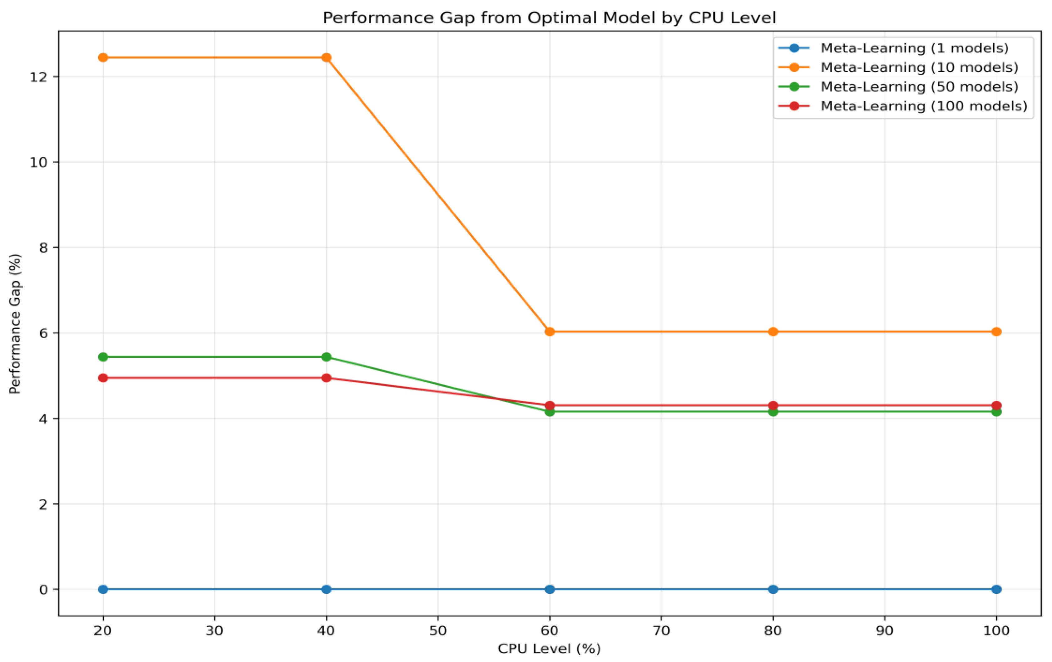
As shown in Figure 5, the performance gap remained negligible for single-sensor cases (close to 0%) and peaked at around 12.4% under 20% CPU resource availability with 10 concurrent sensors. The gap decreased again when the concurrency increased to 50 and 100 sensors, indicating stable generalization through fallback to simpler models. This indicates that the proposal maintains stable and reliable forecasting performance even when operating with limited resources and high service concurrency. The results suggest that although the system selects models under strict resource constraints, it consistently chooses models that are close to optimal in terms of forecasting performance.

The slight increase in the performance gap under heavy sensor loads can be attributed to the system’s resource-aware selection logic. When faced with limited computing capacity, the meta-learner prioritizes inference efficiency, often favoring simpler models over more accurate but computationally intensive ones. Despite this trade-off, the overall accuracy loss remains minor, validating the framework’s ability to intelligently balance accuracy and resource efficiency in real time.

As the available CPU resources increase to 40% or higher, especially when the number of concurrent models reaches 10, the performance gap shows a dramatic reduction. This phenomenon can be explained by the system’s increased capacity to handle computational demands. With more resources, the framework is able to select and execute complex, high-performing models such as TFT, which were previously substituted with simpler models under stricter resource constraints. The number of concurrent models at this level represents a critical threshold where additional CPU availability has a particularly significant impact, as it alleviates resource contention and allows the system to approach optimal model selection accuracy.

4.4.2. Execution Time: Model Selection and Inference

To evaluate the time required to deliver forecasting services under varying resource conditions, we analyzed three components of execution latency: model selection time, inference time, and total service time. These metrics together represent the responsiveness and practicality of the system in delivering forecasting results in real-time environments.

Figure 6 shows the model selection time for both the proposed meta-learning framework and the exhaustive search baseline. The meta-learning approach completed model selection within 0–3 milliseconds across all CPU levels and sensor request sizes. In contrast, the exhaustive search method showed significant selection delays over 100 s, regardless of CPU availability or concurrency level, due to the need to evaluate every model candidate sequentially. This performance gap directly results from the brute-force nature of exhaustive search, which evaluates all candidate models for each sensor sequentially.

The model selection time for the meta-learning framework remained consistently low, completing within approximately 1–2 milliseconds across all CPU levels and sensor request sizes. However, a slight increase in selection time was observed at higher CPU availability levels. This minor variation is unlikely to stem from the model selection logic itself, given its inherently lightweight and rapid design. Instead, it is more plausible that the increase is caused by background processes running on the system’s operating environment. As CPU resources become more available, non-critical background software and system management tasks might opportunistically utilize the excess capacity, leading to subtle but measurable delays in the overall timing of the selection process. Despite this, the impact remains negligible in practice, as the selection time is orders of magnitude shorter than the inference time or total service time.

Figure 7 presents the inference time for the selected forecasting models. While the inference time generally decreased with higher CPU availability, it increased as the number of concurrent models grew due to competition for computational resources. Importantly, the inference time was comparable between the meta-learning and exhaustive methods, since both ultimately execute the same forecasting models after selection. This confirms that inference efficiency is a function of model complexity and resource availability, rather than the selection method itself.

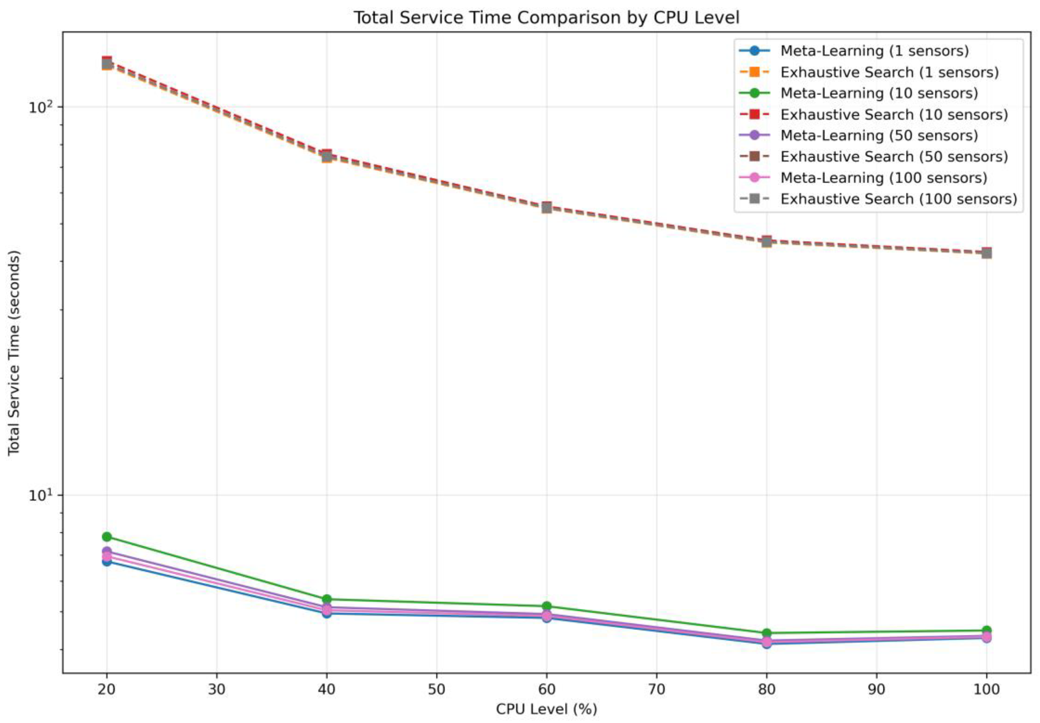
The combined effect of model selection and inference time is summarized in Figure 8, which illustrates the total service time, defined as the duration from receiving a forecasting request to returning the prediction result. The proposed framework consistently completed the full service—including model selection and inference—within 7 to 8 s, even under the most constrained setting of 100 concurrent sensors at 20% CPU. In contrast, the exhaustive search method required over 120 s in total, highlighting its infeasibility for real-time deployment.

These results emphasize the following critical insight: although the inference phase is computationally similar between the two methods, the model selection phase introduces a massive overhead in the exhaustive baseline, severely limiting its feasibility in real-time environments. The proposed system, by reducing the model selection time to near zero, ensures that the end-to-end latency remains within acceptable operational bounds, even as the forecasting demand scales up.

Therefore, in terms of practical deployment in resource-constrained settings, the meta-learning approach offers significant advantages by enabling scalable, low-latency forecasting services with minimal degradation in accuracy.

In contrast, the exhaustive search method required substantially more time, with the total service latency often exceeding 50 to 100 s. This is because exhaustive search evaluates all candidate models before selecting the best one, significantly increasing the model selection time. Although the inference time of each selected model in exhaustive search was often similar to that of the proposed method, the additional overhead from evaluating all models sequentially became the dominant factor in the total latency.

These results clearly demonstrate that the proposed framework achieves low-latency service not by accelerating inference itself but by eliminating the computational burden of exhaustive model selection. The model selection time of the proposed system was consistently under 0.01 s across all settings, enabling fast hand-off to the inference stage. Consequently, inference time becomes the primary latency contributor, but the overall service time remains within operational thresholds for real-time forecasting systems.

Across all tested configurations, the meta-learning framework achieved a total service time speedup ranging from 15× to nearly 19× compared to exhaustive search, enabling practical deployment in latency-sensitive energy control environments.

4.4.3. Model Selection Behavior Analysis

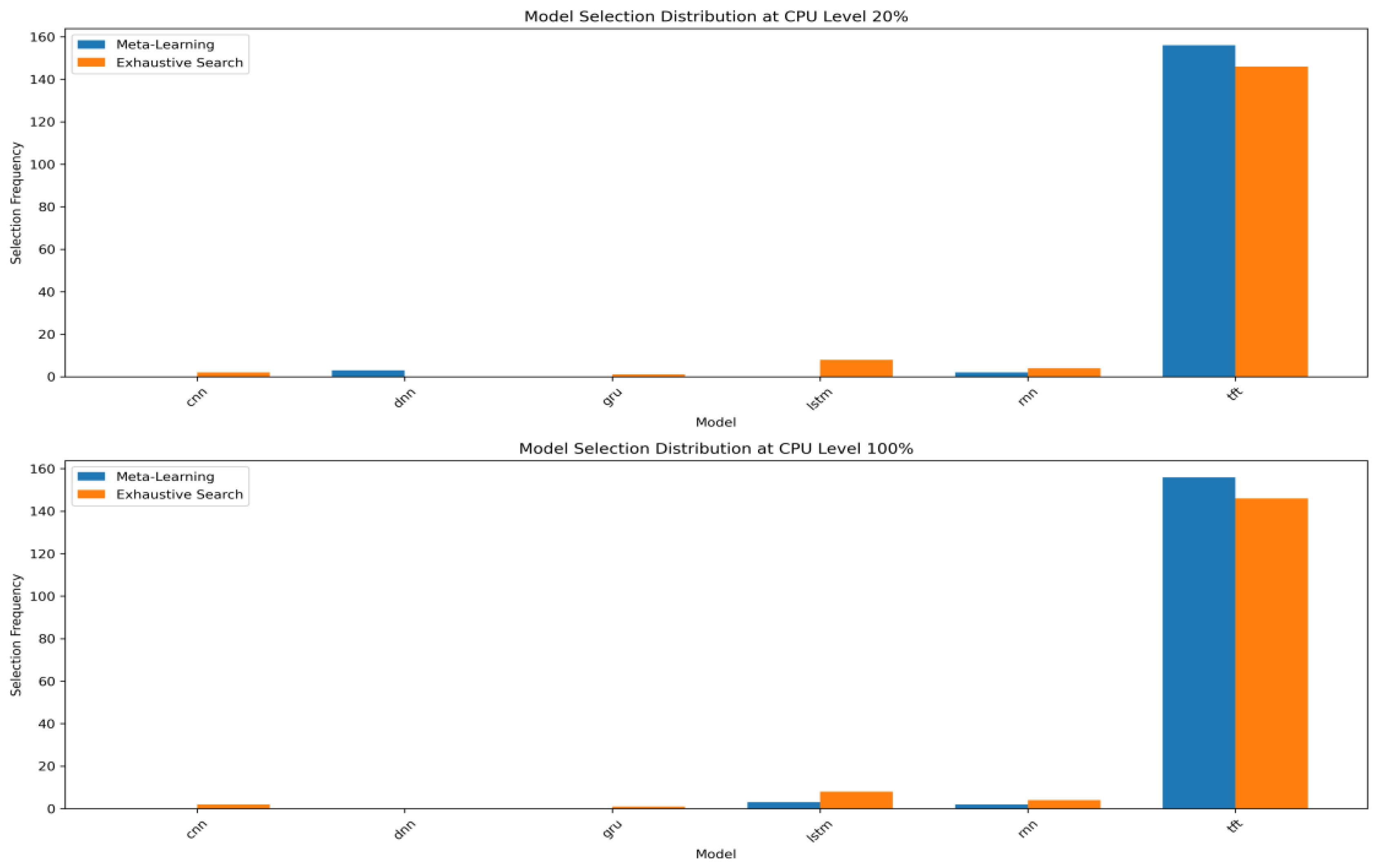
To further understand the behavior of the proposed model selection system, we analyzed the distribution of selected forecasting models at different CPU availability levels. In Figure 9, at both low (20%) and high (100%) CPU levels, the majority of the selected models were TFT, reflecting its high forecasting accuracy in many sensor cases. Interestingly, the meta-learning approach consistently favored TFT, even with low-resource settings, indicating its strong bias toward accuracy over computational cost, which is consistent with our design intent. In contrast, the exhaustive search occasionally selected alternative models such as LSTM and RNN, which may have yielded marginal improvements in latency at the cost of a slight accuracy loss.

This distribution supports the observation that the meta-learning framework, by incorporating performance-based meta-features, tends to select models with historically better results. Moreover, it highlights the need for future refinement to better integrate resource sensitivity into the selection logic.

Table 4. The top five statistical features influencing the model selection.

Feature	Selection Impact (%)
Skewness	35.7
Variance	21.3
Entropy	14.3
Mean	9.9
Max Value	8.2

shows that skewness and variance carry the largest positive SHAP (Shapely Additive exPlanations) contributions for the TFT class; in practical terms, time series exhibiting heavy-tailed or highly dispersed distributions raise the model selection probability of the Transformer by more than 20 percentage points, whereas lower values of these features favor recurrent architectures such as GRU.

4.4.4. Performance Comparison with AutoML-Based Approaches

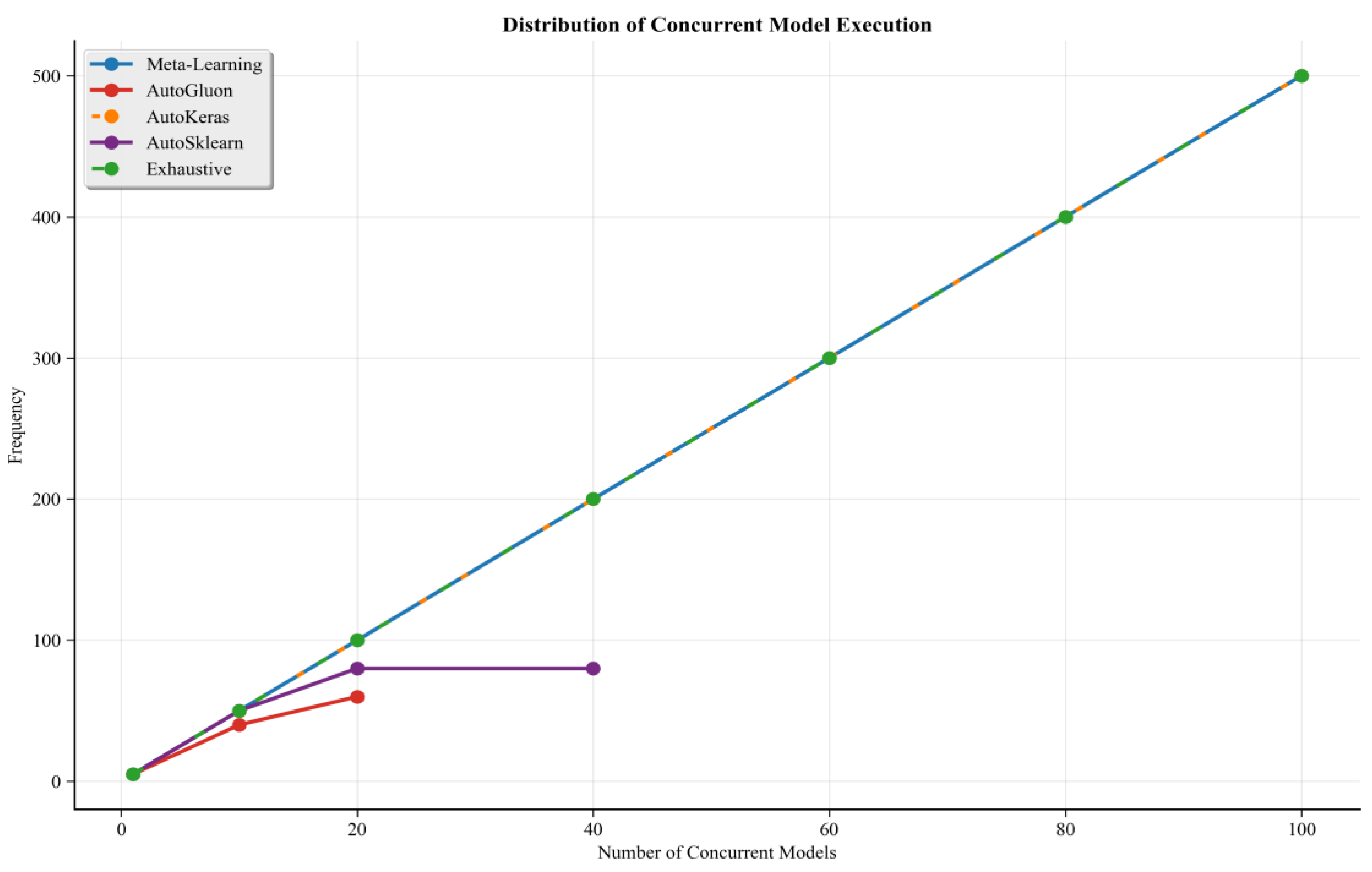
More importantly, we evaluated the scalability limitations of the existing AutoML-based model selection methods under constrained resources. As illustrated in Figure 10, methods such as AutoSklearn, AutoML (AutoKeras), and AutoGluon failed to process the concurrency of model executions that exceeded a certain threshold—typically around 20 to 40 models—regardless of the available CPU levels. This result reflects the heavy computing loads of their model search and selection processes, which often involve repeated retraining, architecture search, and hyperparameter tuning.

In contrast, the proposed meta-learning framework can simultaneously process up to 100 concurrent model executions. As a result, AutoML methods become infeasible for real-time, large-scale deployment in edge environments. These observations underscore the following critical trade-off: although AutoML methods automate model optimization, their scalability limits their applicability in latency-sensitive systems. In contrast, the proposed meta-learning method offers consistent and efficient service performance even under high concurrency and limited resources.

5. Future Work and Limitations

In future work, the proposed framework will be extended to cover a broader range of energy management domains, including electric power usage, renewable energy generation, and multi-source energy integration. While our current experiments are limited to LPG consumption data due to data availability and reliability, the proposed framework is designed to be domain-agnostic. Since it operates on statistical meta-features extracted from time series, the same methodology can be extended to other energy domains, such as electricity, heat, and solar generation. Future validations will be conducted across these domains to assess the generalizability under diverse operational conditions. These domains exhibit diverse time-series patterns and operational constraints, which will require the development of more generalized meta-feature extraction and model selection strategies that can accommodate heterogeneous energy profiles.

Furthermore, to ensure applicability in real-time embedded or edge environments, future research will focus on optimizing the runtime efficiency and adaptability of the framework. This includes developing lightweight meta-models suitable for deployment on constrained devices, incorporating reinforcement learning for dynamic prioritization under varying system loads, and enabling online updating of the meta-learner to reflect temporal drift and changes in forecasting context.

Together, these extensions aim to position the framework as a core component of next-generation intelligent energy control systems that operate autonomously, efficiently, and reliably under practical, real-world conditions.

The current framework is constrained by (i) training data that focus almost exclusively on LPG usage, (ii) unreliable recommendations for cold-start sensors that lack historical data, and (iii) an assumption that meta-features remain stationary within each retraining cycle.

6. Conclusions

This study proposed a meta-learning-based model selection framework for energy digital twin systems that efficiently supports energy management under constrained computing environments. Unlike existing AutoML or static-rule-based methods, the proposed approach dynamically selects an optimal forecasting model for each incoming energy time series, considering both the data characteristics and available computing resources. Through a combination of meta-feature extraction, decision-tree-based classification, and resource-aware selection, the framework enables adaptive and efficient deployment of predictive services.

Comprehensive experiments were conducted using real-world LPG consumption data collected from 566 sensors deployed across various business sites in South Korea. The results demonstrated that the proposed system achieved forecasting accuracy comparable to that of exhaustive search while significantly reducing the model selection and overall service time. Even under the most constrained conditions (e.g., 20% CPU and up to 100 simultaneous requests), the total service time remained under 10 s, confirming the system’s suitability for real-time service deployment.

In particular, the proposed method was shown to eliminate the computational bottleneck of model selection through rapid inference-aware decision logic, achieving a speed amounting to 15 to 19 times that of exhaustive search. These results highlight the practicality and scalability of the framework for real-world energy control scenarios, where rapid response and forecasting reliability are critical. This minor variation is likely due to background processes and non-critical system management tasks utilizing excess CPU resources rather than the selection logic itself. Nonetheless, the selection time remained negligible, ensuring that total service latency was dominated by inference execution rather than model selection overhead.

Future work will explore the integration of reinforcement learning for adaptive prioritization under system load, continual learning of the meta-model to reflect new patterns, and expansion toward multi-modal energy sources beyond LPG. The findings of this work serve as a foundation for intelligent, scalable energy control systems in edge-driven environments.

References

- Adom, P.K. Global Energy-Efficiency Transition Tendencies: Development Phenomenon or Not? Energy Strategy Rev. 2024, 55I, 101524. [Google Scholar]
- Lopez, G.; Pourjamal, Y.; Breyer, C. Paving the Way towards a Sustainable Future or Lagging Behind? An Ex-Post Analysis of the IEA’s World Energy Outlook. Renew. Sustain. Energy Rev. 2025, 212, 115371. [Google Scholar]
- Ba, L.; Tangour, F.; El Abbassi, I.; Absi, R. Analysis of Digital Twin Applications in Energy Efficiency: A Systematic Review. Sustainability 2025, 17, 3560. [Google Scholar] [CrossRef]
- Das, O.; Zafar, M.H.; Sanfilippo, F.; Rudra, S.; Kolhe, M.L. Advancements in Digital Twin Technology and Machine Learning for Energy Systems: A Comprehensive Review of Applications in Smart Grids, Renewable Energy, and Electric Vehicle Optimisation. Energy Convers. Manag. X 2024, 24, 100715. [Google Scholar]
- Han, F.; Du, F.; Jiao, S.; Zou, K. Predictive Analysis of a Building’s Power Consumption Based on Digital Twin Platforms. Energies 2024, 17, 3692. [Google Scholar] [CrossRef]
- Xiang, C.; Li, B.; Shi, P.; Yang, T.; Han, B. Short-Term Photovoltaic Power Prediction Based on a Digital Twin Model. J. Mar. Sci. Eng. 2024, 12, 1219. [Google Scholar]
- Shi, J.; Liu, N.; Huang, Y.; Ma, L. An Edge Computing-Oriented Net Power Forecasting for PV-Assisted Charging Station: Model Complexity and Forecasting Accuracy Trade-Off. Appl. Energy 2022, 310, 118456. [Google Scholar]
- Makridakis, S.; Spiliotis, E.; Assimakopoulos, V. Statistical and Machine Learning forecasting methods: Concerns and ways forward. PLoS ONE 2018, 13, e0194889. [Google Scholar]
- Kontopoulou, V.I.; Panagopoulos, A.D.; Kakkos, I.; Matsopoulos, G.K. A review of ARIMA vs. machine learning approaches for time series forecasting in data driven networks. Future Internet 2023, 15, 255. [Google Scholar]
- Yemets, K.; Izonin, I.; Dronyuk, I. Time Series Forecasting Model Based on the Adapted Transformer Neural Network and FFT-Based Features Extraction. Sensors 2025, 25, 652. [Google Scholar] [CrossRef] [PubMed]
- Kim, J.; Kim, H.; Kim, H.; Lee, D.; Yoon, S. A comprehensive survey of deep learning for time series forecasting: Architectural diversity and open challenges. Artif. Intell. Rev. 2025, 58, 216. [Google Scholar]
- Yıldırım, F.; Yalman, Y.; Bayındır, K.Ç.; Terciyanlı, E. Comprehensive Review of Edge Computing for Power Systems: State of the Art, Architecture, and Applications. Appl. Sci. 2025, 15, 4592. [Google Scholar]
- Chen, J.; Ran, X. Deep learning with edge computing: A review. Proc. IEEE 2019, 7, 1655–1674. [Google Scholar]
- Collopy, F.; Armstrong, J.S. Rule-based forecasting: Development and validation of an expert systems approach to combining time series extrapolations. Manag. Sci. 1992, 38, 1394–1414. [Google Scholar]
- Prudêncio, R.B.; Ludermir, T.B. Meta-learning approaches to selecting time series models. Neurocomputing 2004, 61, 121–137. [Google Scholar]
- Shchur, O.; Turkmen, A.C.; Erickson, N.; Shen, H.; Shirkov, A.; Hu, T.; Wang, B. AutoGluon–TimeSeries: AutoML for probabilistic time series forecasting. In Proceedings of the International Conference on Automated Machine Learning, Berlin, Germany, 12–15 November 2023. [Google Scholar]
- Jin, H.; Song, Q.; Hu, X. Auto-keras: An efficient neural architecture search system. In Proceedings of the 25th ACM SIGKDD International Conference on Knowledge Discovery Data Mining, Anchorage, AK, USA, 4–8 August 2019; pp. 1946–1956. [Google Scholar]
- Talkhi, N.; Akhavan Fatemi, N.; Jabbari Nooghabi, M.; Soltani, E.; Jabbari Nooghabi, A. Using meta-learning to recommend an appropriate time-series forecasting model. BMC Public Health 2024, 24, 148. [Google Scholar]
- Fischer, R.; Saadallah, A. AutoXPCR: Automated multi -objective model selection for time series forecasting. In Proceedings of the 30th ACM SIGKDD Conference on Knowledge Discovery and Data Mining, Barcelona, Spain, 25–29 August 2024; pp. 806–815. [Google Scholar]
- Yao, Y.; Li, D.; Jie, H.; Li, T.; Chen, J.; Wang, J.; Li, F.; Gao, Y. SimpleTS: An efficient and universal model selection framework for time series forecasting. Proc. VLDB Endow. 2023, 16, 3741–3753. [Google Scholar]
- Kozielski, M.; Henzel, J.; Wróbel, Ł.; Łaskarzewski, Z.; Sikora, M. A sensor data-driven decision support system for liquefied petroleum gas suppliers. Appl. Sci. 2021, 11, 3474. [Google Scholar]
- Alexandrov, A.; Benidis, K.; Bohlke-Schneider, M.; Flunkert, V.; Gasthaus, J.; Januschowski, T.; Maddix, D.C.; Rangapuram, S.; Salinas, D.; Schulz, J. Gluonts: Probabilistic and neural time series modeling in python. J. Mach. Learn. Res. 2020, 21, 1–6. [Google Scholar]