Improved Hybrid A* Algorithm Based on Lemming Optimization for Path Planning of Autonomous Vehicles

Abstract

Path planning for autonomous vehicles is a core component of intelligent transportation systems, playing a key role in ensuring driving safety, improving driving efficiency, and optimizing the user experience. To address the challenges of safety, smoothness, and search efficiency in path planning for autonomous vehicles, this study proposes an improved hybrid A* algorithm based on the lemming optimization algorithm (LOA). Firstly, this study introduces a penalized graph search method, improves the distance heuristic function, and incorporates the Reeds–Shepp algorithm in order to overcome the insufficient safety and smoothness in path planning originating from the hybrid A* algorithm. The penalized graph search method guides the search away from dangerous areas through penalty terms in the cost function. Secondly, the distance heuristic function improves the distance function to reflect the actual distance, which makes the search target clearer and reduces the computational overhead. Finally, the Reeds–Shepp algorithm generates a path that meets the minimum turning radius requirement. By prioritizing paths with fewer reversals during movement, it effectively reduces the number of unnecessary reversals, thereby optimizing the quality of the path. Additionally, the lemming optimization algorithm (LOA) is combined with a two-layer nested optimization framework to dynamically adjust the key parameters of the hybrid A* algorithm (minimum turning radius, step length, and angle change penalty coefficient). Leveraging the LOA’s global search capabilities avoids local optima in the hybrid A* algorithm. By combining the improved hybrid A* algorithm with kinematic constraints within a local range, smooth paths that align with the actual movement capabilities are generated, ultimately enhancing the path search capabilities of the hybrid A* algorithm. Finally, simulation experiments are conducted in two scenarios to validate the algorithm’s feasibility. The simulation results demonstrate that the proposed method can efficiently avoid obstacles, and its performance is better than that of the traditional hybrid A* algorithm in terms of the computational time and average path length. In a simple scenario, the search time is shortened by 33.2% and the path length is reduced by 11.1%; at the same time, in a complex scenario, the search time is shortened by 23.5% and the path length is reduced by 13.6%.

1. Introduction

Autonomous vehicles are equipped with advanced sensors, controllers, and actuators to perceive complex environments, make intelligent decisions, and execute motion control, ultimately achieving human-like driving performance [1,2]. Path planning, as an indispensable component of autonomous driving systems [3], relies on environmental data from perception layers and transmits planned trajectories to control layers for execution [4]. A fast and robust planning layer directly impacts the performance of autonomous vehicles.

In recent years, path planning algorithms have rapidly evolved and can be broadly categorized into five types [5].

(1)

Graph Search-Based Algorithms

The principle of grid-based search algorithms involves discretizing the entire map by dividing it into a number of grids or cells. The vehicle then selects its start and end points based on its needs and plans a path through these cells according to the cost, with the path generated via connections between the cells. This category of algorithms primarily includes the Dijkstra and A* algorithms, among others. Dijkstra [6] is a single-source shortest-path optimal path planning algorithm. In Dijkstra, the state space is typically discretized into grid cells before searching [7]. Zhu et al. [8] proposed the Reverse Labeling Dijkstra Algorithm (RLDA) to solve this problem, theoretically proving its correctness and demonstrating its low polynomial time complexity. Sang et al. [9] introduced an alternative implementation of the A* algorithm. By incorporating grid obstacle rates into the evaluation function and enhancing the heuristic function, this method improves the search efficiency and path smoothness. Zhou [10] introduced an improved A* algorithm that incorporates the salp swarm algorithm (SSA) for heuristic function optimization and proposed improved B-spline interpolation for path smoothing. Although grid-based search algorithms are easy to implement, they face several challenges during the search process: high computational complexity, limited path accuracy, difficulty in adapting to dynamic environments, an inability to directly account for vehicle kinematic constraints, and heightened sensitivity to perception errors.

(2)

Sampling-Based Algorithms

The principle of sampling-based path planning algorithms involves generating a set of sample points in the feasible space through random or strategic sampling and then constructing connections among these points to form a feasible path from the start to the goal.

Representative algorithms in this category include rapidly exploring random trees (RRT) and probabilistic roadmaps (PRM). Hao [11] proposed combining an improved artificial potential field method with the RRT algorithm for path planning. This hybrid approach utilizes RRT’s obstacle avoidance capability to address path oscillation issues. Cao et al. [12] modified the sampling strategy of the conventional PRM by implementing uniform sampling in obstacle-dense regions while increasing the sampling points in narrow passages, thereby improving the traversal success rates in constrained spaces while achieving shorter path lengths and reduced traversal times. While sampling-based algorithms demonstrate superior computational efficiency in high-dimensional spaces, their generated paths often lack smoothness. Particularly in dense obstacle environments, they exhibit slower convergence rates and tend to produce suboptimal solutions.

(3)

Interpolation-Based Algorithms

Interpolation-based planning algorithms [13] operate by generating smooth intermediate waypoints between the start and goal points; then, mathematical interpolation methods are applied to construct constrained smooth trajectories, which ensures feasibility and continuity. The interpolation-based approaches include polynomial interpolation, spline interpolation, Bézier curve interpolation, and curvature-continuous interpolation. Zhu [14] employed the Ramer–Douglas–Peucker (RDP) algorithm [15] to compress the path waypoints and then used polynomial fitting between adjacent waypoints to ensure smooth vehicle motion. Critical collision-prone segments were subsequently refined through interpolation. Li [16] proposed an effective trajectory generation algorithm to shorten and smooth jerky paths obtained from sampling-based planners in cluttered environments. This method utilizes cubic B-splines to represent collision-free trajectories with strict continuity while respecting velocity/acceleration constraints. Zheng [17] developed an autonomous vehicle trajectory planning algorithm combining quartic Bézier curves with risk potential fields. A potential field function evaluates the collision risk for candidate paths to generate collision-free trajectories. These algorithms depend heavily on the distribution and quality of known data points. Sparse or unevenly distributed data may cause significant errors, posing challenges for high-dimensional or nonlinear complex problems.

(4)

Numerical Optimization-Based Algorithms

Numerical optimization-based planning algorithms [18] obtain optimal paths or strategies by numerical optimization. There are various types of numerical optimization-based planning algorithms, with the most commonly used including dynamic programming (DP), model predictive control (MPC), genetic algorithms (GAs), and particle swarm optimization (PSO). Hu [19] proposed an event-triggered model predictive adaptive dynamic programming (MPADP) algorithm to plan the path of an unmanned ground vehicle (UGV) at road intersections. The actor–critic scheme of adaptive dynamic programming (ADP) combined cost function approximation and control policy generation to formulate MPADP. Ji [20] introduced a path planning and tracking framework to ensure collision-free trajectories for autonomous vehicles. For the path planning method, a 3D virtual danger potential field was constructed by superimposing trigonometric functions for roads and exponential functions for obstacles, generating the desired collision avoidance trajectories when potential collisions are detected. Li [21] proposed an AGV path planning method based on an artificial potential field–ant colony algorithm, which improves the performance of the algorithm by incorporating the artificial potential field for the construction of a potential field heuristic function and dynamically adjusting the pheromone fluctuation coefficients, introducing multiple parameters to dynamically adjust the pheromone increment, and optimizing the paths with the pruning method. Despite their advantages, numerical optimization-based planning algorithms are highly sensitive to the initial values, prone to local optima, and suffer from high computational complexity in high-dimensional or nonlinear problems, which influences their real-time performance and global optimality.

(5)

Machine Learning-Based Algorithms

Machine learning-based planning algorithms train models to learn environmental features and decision-making strategies from data. The trained models are then used to predict or generate optimal paths or actions in order to achieve adaptive and intelligent path planning. Machine learning methods that have been applied in the planning domain include neural networks [22], reinforcement learning [23], deep learning [24], and end-to-end learning [25]. The limitations of machine learning-based planning algorithms lie in their strong dependence on training data, limited generalization capabilities, high computational complexity, and potential challenges in interpretability and safety assurance in practical applications.

A mixed-integer programming algorithm is an algorithm that combines multiple optimization techniques and methods to solve complex optimization problems. It typically combines classical mathematical programming methods (such as linear programming and integer programming) with modern heuristic algorithms (such as genetic algorithms and particle swarm optimization) or other artificial intelligence technologies.

Combining mathematical programming with heuristic algorithms effectively solves the computational complexity problem of traditional hybrid A* algorithms in high-dimensional state space searches by combining the accuracy of mathematical programming with the efficient search capabilities of heuristic algorithms [26].

Hybrid meta-heuristic algorithms significantly improve the performance of path planning problem solving by synergistically integrating the complementary advantages of multiple optimization mechanisms [27].

The integration of machine learning and planning algorithms has formed a new generation of intelligent path planning paradigms whose core goal is to enhance the adaptability and intelligence of traditional planning algorithms through data-driven methods [28].

Multi-objective mixed programming achieves a dynamic balance between safety, efficiency, and comfort by constructing a hierarchical optimization system [29].

The latest developments in the application of mixed-integer programming algorithms and optimization techniques in actual autonomous driving systems are listed in

Table 1. Application of mixed programming algorithms in autonomous driving systems.

Algorithm Type	Core Technology	Advantageous Scenarios	Application
Layered planning framework	Hybrid A* + MPC	Structured roads	Benz DRIVEPILOT3.0
Deep learning-driven	BEV-Transformer	Complex urban road conditions	Huawei ADS 3.0
Hybrid enhancement	RRT + reinforcement learning	Extreme obstacle scenarios	Waymo Driver 5
End-to-end architecture	Multimodal large model	Adaptation to all scenarios	Tesla Dojo platform

.

By embedding natural group intelligence strategies into traditional path planning frameworks, this improvement not only enhances the algorithm performance but also sets new standards for the reliability of autonomous driving in extreme scenarios, demonstrating the cutting-edge value of the fusion of bionics and artificial intelligence.

The development of optimization algorithms is one of the core drivers of the evolution of autonomous driving technology. Combining optimization algorithms not only improves the quality and efficiency of path planning but also pushes the whole system towards higher-order automation and intelligence [30]. Optimization algorithms can be classified into the following six categories: learning-enhanced optimization, distributed collaborative optimization, quantum-inspired optimization, bio-inspired intelligent optimization, robust stochastic optimization, and lightweight real-time optimization. Currently, the most popular application is bio-inspired intelligent optimization, which is achieved by simulating the intelligent behavior of biological populations or physical phenomena in nature [31].

Table 2. Comparison of optimization algorithms’ characteristics.

Algorithm	Advantages	Drawbacks	Applicable Scenarios
LOA	Strong global search capabilities for high-dimensional optimization problems	Slow convergence Sensitive parameter tuning	Multi-objective optimization problems Path planning
GWO	Simple structure with few parameters Fast convergence	Easy to fall into local optimality Strong dependence on initial population	Continuous space optimization Engineering design problems
SCA	Clear mathematical principles No gradient information required	Weak development capabilities Poor adaptability to dynamic environments	Low-dimensional nonlinear optimization Initial path generation
Hybrid A* algorithm	High path feasibility Better real-time performance	Higher computational complexity Insufficient path smoothing	Autopilot path planning Motion planning

compares several optimization algorithms.

In summary, the challenges faced by autonomous vehicle path planning include low efficiency during path searches, safety issues between vehicles and other objects, and the final insufficiently smooth path curve. Therefore, this paper proposes an improved hybrid A* algorithm based on lemming optimization. First, the distance function of the improved hybrid A* algorithm is enhanced to improve the efficiency. Second, the lemming optimization algorithm is integrated to improve the path curve smoothness and reduce the computational load. The main goals of this work are (1) to ensure the safety of the vehicle path by setting a safe distance from obstacles and to select the optimal node in the path search by choosing an appropriate distance heuristic function and increasing the angle penalty coefficient to improve the search efficiency; (2) to perform a global search using the lemming optimization algorithm, update the population using the migration, competition, and reproduction mechanisms of the lemming optimization algorithm, and iteratively optimize the key parameters of the improved hybrid A* algorithm; (3) to use the paths generated by the lemming optimization algorithm as heuristic information to guide the search direction of the hybrid A* algorithm, consider the vehicle’s kinematic constraints (such as steering angle and speed limits) during the search process, and, finally, ensure the safety, smoothness, and efficiency of the generated paths. The workflow of the fused algorithm is illustrated in Figure 1.

This paper is structured as follows: Section 2 provides an overview of the overall structure of the hybrid A* algorithm and the lemming optimization algorithm; Section 3 describes the improvements made to the distance heuristic function and penalty function of the hybrid A* algorithm; Section 4 introduces the fusion principle of the hybrid path planning algorithm and the integration mechanism of path combinations; Section 5 presents simulation experiments and analyzes the results; and Section 6 summarizes the work of this study and considers potential future research directions.

2. Algorithm Overview

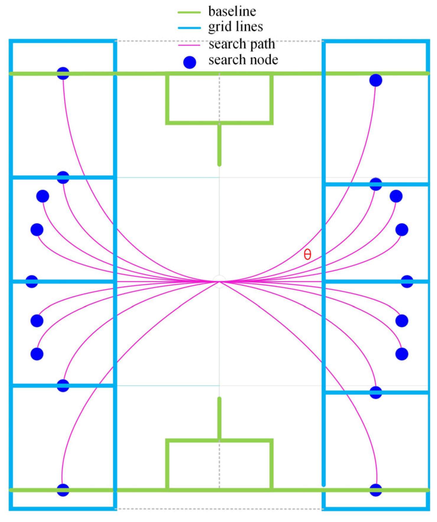
2.1. Hybrid A* Algorithm

The hybrid A* algorithm effectively integrates a discrete search with a continuous state space, balancing path smoothness and computational efficiency through a grid discretization strategy while accounting for vehicle kinematic constraints and θ-direction exploration. This approach generates paths that combine motion feasibility with obstacle avoidance capabilities. Its discretization mechanism not only ensures a bounded search space but also maintains algorithmic efficiency. The hybrid A* search process is illustrated in Figure 2.

2.2. Lemming Optimization Algorithm

The LOA is a bio-inspired metaheuristic algorithm that leverages the migratory behavior of lemmings for intelligent optimization [32]. Inspired by the collective migration and unique behavioral traits of lemming populations, this algorithm simulates their exploratory, following, and jumping dynamics in complex environments. By emulating this swarm intelligence, the algorithm continuously adjusts and optimizes individual positions within the search space, progressively guiding them towards the global optimum—akin to how lemmings rely on instinct and collaboration to navigate optimal survival paths in nature.

2.2.1. Position Initialization

Before entering the iterative process, the LOA initializes the positions of all search agents. The initial candidate solutions are represented as a matrix $\overrightarrow{Z}$ with dimensions $N$ × $Dim$ (where $N$ is the population size and $Dim$ is the problem dimensionality), bounded by the lower and upper limits of the search space. This is formulated as in Equation (1):

$$\overrightarrow{Z}=\left[\begin{array}{ccccc}{z}_{1,1}& z_{1,2}& \dots & z_{1,Dim-1}& z_{1,Dim}\\ z_{2,1}& z_{2,1}& \dots & z_{2,Dim-1}& z_{2,Dim}\\ \dots & \dots & z_{ij}& \dots & \dots \\ ⋮& ⋮& ⋮& ⋮& ⋮\\ z_{N-1,1}& z_{N-1,2}& \dots & z_{N-1,Dim-1}& z_{N-1,Dim}\\ z_{N,1}& z_{N,2}& \dots & z_{N,Dim-1}& z_{N,Dim}\end{array}\right]$$

(1)

In each iteration, the best position determined is considered to be the optimal solution or approximately optimal solution obtained so far. The decision variables $Z_{\mathrm{i},\mathrm{j}}$ for each dimension are calculated according to Equation (2):

$$z_{ij}=L{B}_j+rand\times \left(U{B}_j-L{B}_j\right),i=1,2,\dots ,N,j=1,2,\dots ,Dim$$

(2)

where this value is a random number between 0 and 1.; $L{B}_{\mathrm{j}}$ is used to represent the lower limit of the $j^{th}$ dimension, $U{B}_j$ and $j^{th}$ simultaneously represent the upper limit of the dimension.

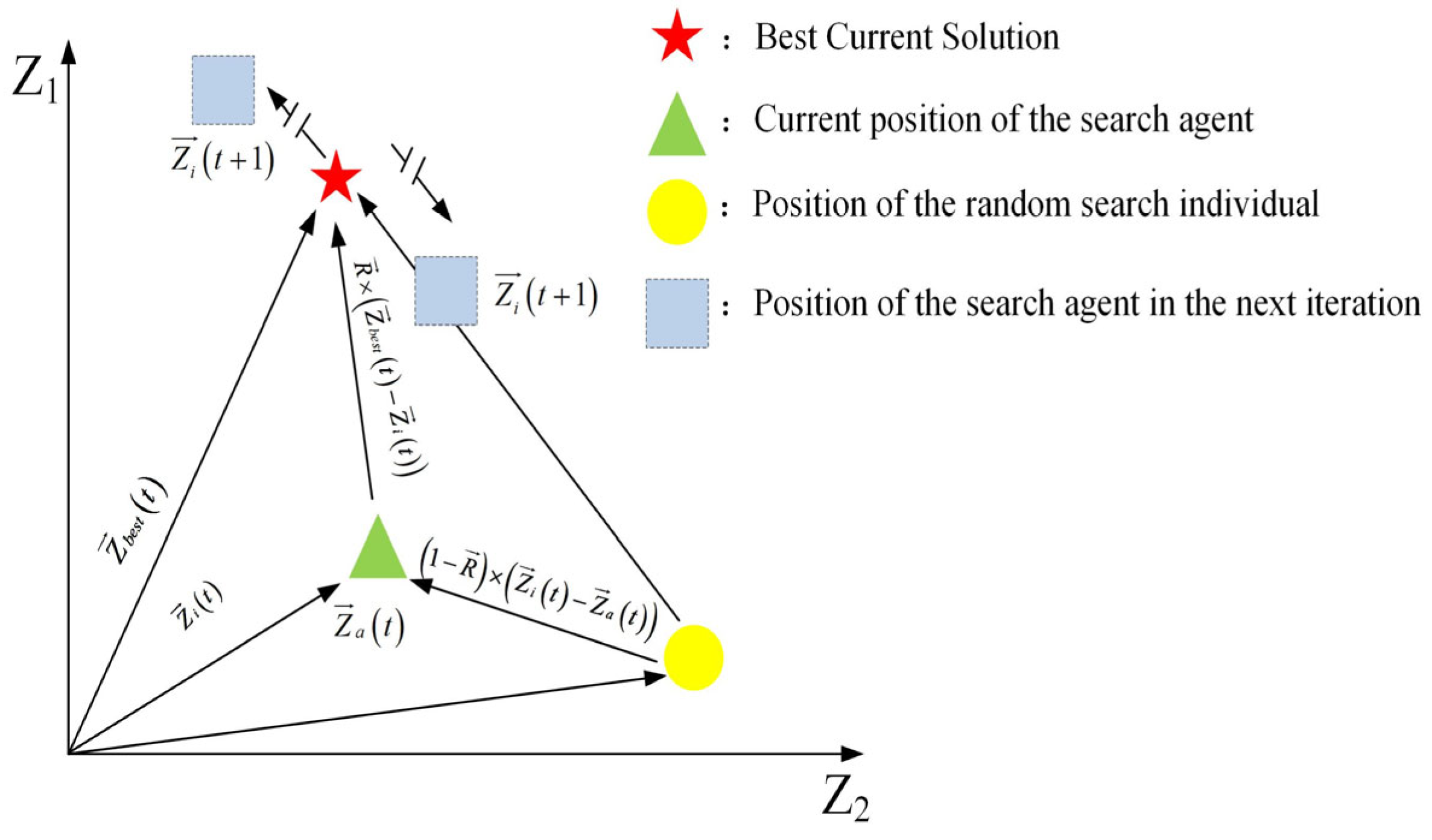
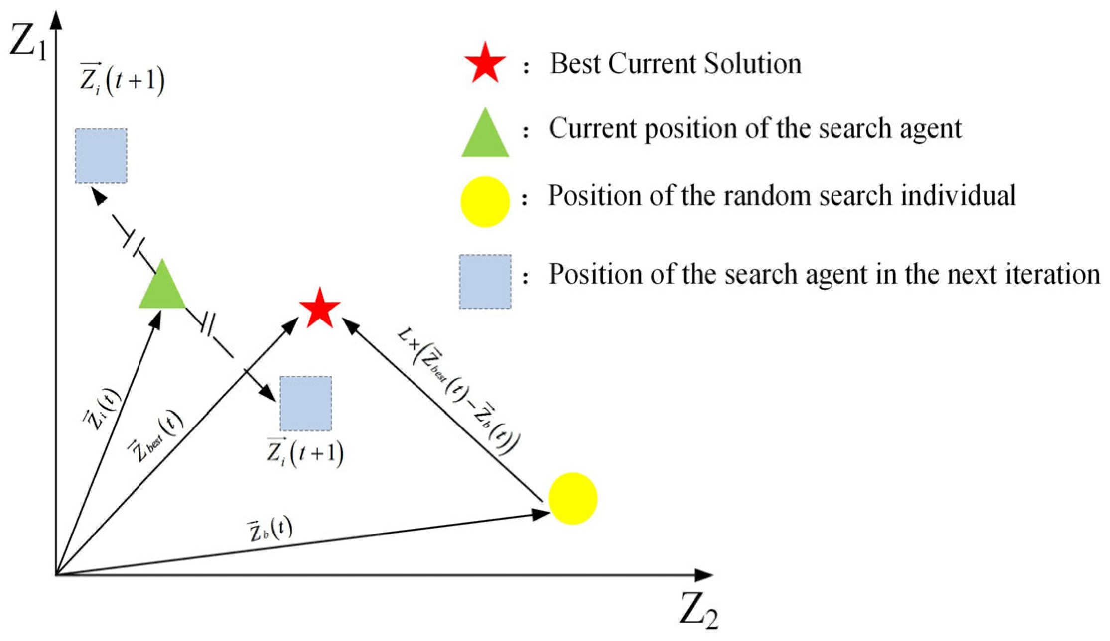
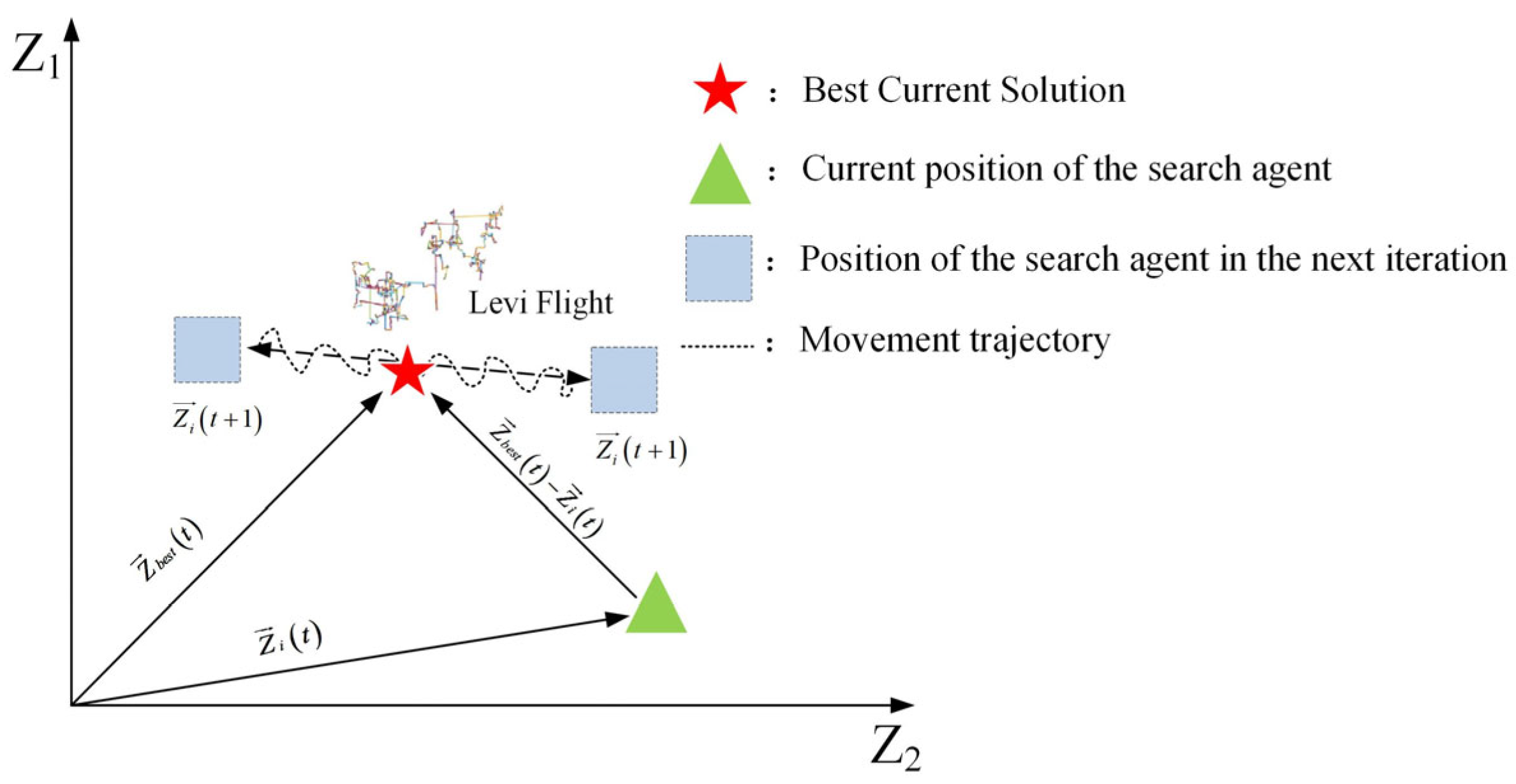
2.2.2. Behavioral Patterns

Lemmings exhibit four key behaviors. They migrate across long distances, dig complex burrow systems, constantly search for food sources, and use various methods to escape predators.

(1)

Long-distance migration

Lemmings explore their surroundings based on their current locations and the positions of random individuals within their populations, seeking habitats that are abundant in food sources to secure better living conditions and resources. Notably, factors such as the ecological conditions influence their migration, in which both the direction and distance of their movement are not fixed. This behavior can be modeled using the following Equation (3):

$$\overrightarrow{Z_i}\left(t+1\right)={\overrightarrow{Z}}_{best}\left(t\right)+F\times \overrightarrow{BM}\times \left(\overrightarrow{R}\times \left({\overrightarrow{Z}}_{best}\left(t\right)-{\overrightarrow{Z}}_i\left(t\right)\right)+\left(1-\overrightarrow{R}\right)\times \left({\overrightarrow{Z}}_i\left(t\right)-{\overrightarrow{Z}}_a\left(t\right)\right)\right)$$

(3)

where $\overrightarrow{Z_{\mathrm{i}}}(t+1)$ denote the $ith$ position of the search agent during iteration $(t+1)$,while ${\overrightarrow{Z}}_{best}(t)$ indicates the current global optimum solution. The direction control parameter $F$, calculated as in Equation (5), facilitates exploration by periodically altering the search trajectories to escape local optima. The stochastic component $\overrightarrow{BM}$ implements Brownian motion with step sizes derived from a normal distribution—see Equation (4)—enabling dynamic space exploration. Additionally, $\overrightarrow{R}$ represents a uniformly distributed random vector [−1,1] (where d is the problem dimensionality), generated via Equation (6), which enhances the solution space coverage. ${\overrightarrow{Z}}_i(t)$ denotes the position vector of the $ith$ search agent, while ${\overrightarrow{Z}}_{\mathrm{a}}(t)$ represents a randomly chosen individual from the population. The integer parameter a is between 1 and $N$. governs the directional movement between the current optimal solution and randomly selected individuals, mathematically characterizing the inter-agent interactions during migration. The two-dimensional mathematical representation of this long-distance migration mechanism is depicted in Figure 3.

$$f_{BM}\left(x;0,1\right)={\displaystyle \frac{1}{\sqrt{2\pi }}}\times \exp \left(-{\displaystyle \frac{x^2}{2}}\right)$$

(4)

$$F=\left\{\begin{array}{cc}1\hfill & if\left[2\times rand+1\right]=1\hfill \\ -1\hfill & if\left[2\times rand+1\right]=2\hfill \end{array}\right.$$

(5)

$$\overrightarrow{R}=2\times rand\left(1,Dim\right)-1$$

(6)

(2)

Digging holes

The second behavior of lemmings is the digging of burrows in their habitats, forming complex tunnels that provide safe shelter and storage for food. Lemmings will randomly dig new burrows based on the current location of the burrow and the locations of random individuals in the population. This design assists them in quickly escaping the threats of predators and searching for food more efficiently. The burrowing behavior is mathematically modeled as in Equation (7), with Figure 4 providing a simplified schematic representation.

$${\overrightarrow{Z}}_i\left(t+1\right)={\overrightarrow{Z}}_i\left(t\right)+F\times L\times \left({\overrightarrow{Z}}_{best}\left(t\right)-{\overrightarrow{Z}}_b\left(t\right)\right)$$

(7)

where $L$ represents an iteration-dependent stochastic parameter, while ${\overrightarrow{Z}}_b$ denotes a randomly sampled population member. The discrete control parameter b is between 1 and $N$. $L$ and ${\overrightarrow{Z}}_b$ represent the interaction between the solution vectors during the adjustment process. Figure 4 illustrates the burrowing behavior model, where $L$ is computed as follows:

$$L=rand\times \left(1\times \sin \left({\displaystyle \frac{t}{2}}\right)\right)$$

(8)

(3)

Gathering food

The third behavioral pattern involves lemmings exhibiting extensive stochastic movement within their burrow systems, utilizing their highly developed olfactory and auditory capabilities to detect nutritional resources. Typically, lemmings establish a constrained foraging radius proportional to the local food density and accessibility. To maximize resource acquisition, they employ a random walk strategy when exploring their designated feeding zones. The mathematical representation of this foraging behavior is provided in Equation (9), with Figure 5 illustrating the corresponding movement patterns.

$${\overrightarrow{Z}}_i\left(t+1\right)={\overrightarrow{Z}}_{best}\left(t\right)+F\times spiral\times rand\times {\overrightarrow{Z}}_i\left(t\right)$$

(9)

where $spiral$ characterizes the helical exploration trajectory employed during foraging activities, with its mathematical formulation being governed by Equations (10) and (11):

$$spiral=radius\times \left(\sin \left(2\times \pi \times rand\right)+\cos \left(2\times \pi \times rand\right)\right)$$

(10)

$$radius=\sqrt{{\displaystyle \sum _{j=1}^{Dim}{\left(z_{best}{,}_j\left(\mathrm{t}\right)-z_i{,}_j\left(t\right)\right)}^2}}$$

(11)

where $radius$ represents the radius of the foraging range and also represents the Euclidean distance between the current location and the best solution.

(4)

Evading predators

The terminal phase of the model captures lemmings’ predator evasion strategies, wherein burrows function as the primary refuge sites. Upon threat detection, lemmings leverage their exceptional sprint capacity to retreat to subterranean shelters while executing stochastic escape trajectories (e.g., sudden directional changes or feints) to disrupt predator pursuit. This predator–prey dynamic is formalized in Equation (12), with Figure 6 providing a schematic representation of the evasion mechanics.

$${\overrightarrow{Z}}_{\mathrm{i}}\left(t+1\right)={\overrightarrow{Z}}_{best}\left(t\right)+F\times G\times Levy\left(Dim\right)\times \left({\overrightarrow{Z}}_{best}\left(t\right)-{\overrightarrow{Z}}_i\left(t\right)\right)$$

(12)

$$G=2\times \left(1-{\displaystyle \frac{t}{T_{\max }}}\right)$$

(13)

where $G$ represents the escape coefficient of lemmings, reflecting their ability to evade threats. This coefficient diminishes as the number of iterations grows, as detailed in Equation (13). Additionally, $T_{\max }$ indicates the maximum number of iterations.

To model the deceptive movements of lemmings during their escape, $Levy(x)$ represents the $Levy$ flight function. This stochastic mechanism captures the irregular and sudden shifts in their trajectories. The mathematical expression for the $Levy$ flight function is provided in Equation (14):

$$Levy\left(x\right)=0.01\times {\displaystyle \frac{u\times \sigma }{{\left|v\right|}^{\frac{1}{\beta }}}},\sigma ={\left({\displaystyle \frac{\Gamma \left(1+\beta \right)\times \sin \left(\frac{\pi \beta }{2}\right)}{\Gamma \left(\frac{1+\beta }{2}\right)\times \beta \times 2^{\left(\frac{\beta -1}{2}\right)}}}\right)}^{{\displaystyle \frac{1}{\beta }}}$$

(14)

where $u$ and $v$ are random numbers in the compartment between 0 and 1, and $\beta$ is an unchanging number equal to 1.5.

3. Improved Hybrid A* Algorithm

The traditional hybrid A* algorithm significantly increases the computational complexity due to the need for the high-dimensional discretization search of the position and heading angle in a continuous space. Additionally, its limitations in terms of local kinematic constraints can easily cause sudden changes in path curvature and frequent direction changes, resulting in inherent deficiencies in the global path smoothness and control efficiency. In response to the above issues, this paper proposes the following improvements to the hybrid A* algorithm.

3.1. Distance Heuristic Function

In the hybrid A* algorithm, distance heuristics are used to estimate the cost from the current node to the target node, helping the path to converge towards the target. These heuristics typically combine multiple estimation methods, taking into account the vehicle’s kinematic constraints and environmental information to generate the shortest and most feasible path. Common distance heuristics include the following.

(1)

Manhattan distance:

$$H\left(\mathrm{n}\right)=\left|x_n-x_{goal}\right|+\left|y_n-y_{goal}\right|$$

(15)

The Manhattan distance refers to the sum of the horizontal and vertical distances between the current node and the target node.

(2)

Euclidean distance:

$$H\left(n\right)=\sqrt{{\left(x_n-x_{goal}\right)}^2+{\left(y_n-y_{goal}\right)}^2}$$

(16)

The Euclidean distance represents the straight-line distance between the current node $(x_n,y_n)$ and the target node $(x_{goal},y_{goal})$.

The search performance of the hybrid A* algorithm is influenced by the heuristic $H(n)$. When $H(n)$ is closer to the true cost, the total computational cost decreases, and the search efficiency improves. However, in practice, it is difficult to accurately estimate the value of $H(n)$. The Manhattan distance, which is the sum of the horizontal and vertical distances, is often much larger than the actual distance, while the Euclidean distance, representing the straight-line distance between two points, does not account for the realistic constraints of vehicle movement. Therefore, a middle value between the Manhattan distance and the Euclidean distance can be adopted as the heuristic estimate $H(n)$. In Figure 7, the diagonal segment represents the Euclidean distance, while the dashed segment denotes an intermediate value between the Manhattan distance and the Euclidean distance. The improved H(n) estimate is illustrated in Figure 7.

(1)

When d₁ = d₂

$$H^{*}\left(n\right)=\sqrt{{d_1}^2+{d_2}^2}=\sqrt{2}{d}_2$$

(17)

(2)

When d₁ > d₂

$$H^{*}\left(n\right)=\sqrt{2{d_2}^2}+d_1-d_2=\left(\sqrt{2}-1\right)d_2+d_1$$

(18)

(3)

When d₁ < d₂

$$H^{*}\left(n\right)=\left(\sqrt{2}-1\right)d_1+d_2$$

(19)

In summary, the expression for $H^{*}\left(n\right)$ is as shown in Equation (20):

$$H^{*}\left(n\right)=\left\{\begin{array}{c}\left(\sqrt{2}-1\right)d_2+d_1\hspace{1em}{d}_1\ge d_2\\ \left(\sqrt{2}-1\right)d_1+d_2\hspace{1em}{d}_1<d_2\end{array}\right.$$

(20)

where the calculation formulas for $d_1$ and $d_2$ are as shown below in Equation (21); $d_1$ and $d_2$ represent distances in a two-dimensional plane. $N(x_n,y_n)$ denotes the coordinates of the current node, and $G(x_{goal},y_{goal})$ represents the coordinates of the target point.

$$\left\{\begin{array}{c}{d}_1=\left|x_{goal}-x_n\right|\\ d_2=\left|y_{goal}-y_n\right|\end{array}\right.$$

(21)

3.2. Steering Penalty Term

In the hybrid A* algorithm, the steering penalty term is used to restrict unnecessary sharp turns in the path, ensuring smoother and more feasible trajectories that comply with the vehicle’s kinematic constraints, as shown in the following Equation (22):

$$g\left(n\right)=g\left(n-1\right)+s+P_{\theta }\cdot {\displaystyle \sum \left|{\theta }_n-{\theta }_{n-1}\right|}$$

(22)

where $g(n)$ represents the total cost of the current node; $g(n-1)$ denotes the total cost of the previous node; $S$ indicates the step length (unit movement distance); $P_{\theta }$ is the steering penalty coefficient (range: [0.1, 5]); while ${\theta }_n$ and ${\theta }_{n-1}$ represent the heading angles (in radians) of the current and previous nodes. During path searching, excessive steering angle changes result in higher costs, prompting the algorithm to prioritize smoother paths.

Different types of penalty functions are used at different stages of the algorithm. Compared with hybrid A*, the penalty functions are as shown in

Table 3. The role of penalty functions in hybrid A*.

Type of Punishment	Effect	Technical Implementation
Incomplete constraint penalty	Ensures that the path complies with the vehicle kinematics	Reeds–Shepp curve generation Hermit satisfaction
Obstacle collision penalty	Avoid paths that cross obstacles	Grid map (sign) and continuous monitoring (isPathClear)
Path length penalty	Prefers shorter paths	Fitness function (length_penalty)

.

Therefore, as can be seen from Table 3, the penalty function in hybrid A* restricts drastic changes in the turning angle when calculating the cost. If the angle changes too much, the cost increases, preventing the algorithm from making large, frequent direction changes during obstacle avoidance, thereby avoiding excessive sharp turns.

3.3. Reeds–Shepp Curves

The Reeds–Shepp curve is a tool used for the path planning of nonholonomic constrained vehicles, capable of generating the shortest feasible paths that allow both forward and backward motion. They extend Dubins curves (which permit only forward movement) and are applicable to vehicles with minimum turning radius constraints. The calculation of the Reeds–Shepp curve is as shown in Equation (23):

$$d=\min {\displaystyle \sum d_i}$$

(23)

where $d$ represents the total path length; $d_i$ denotes the segment length of the path, where each segment may consist of straight-line driving, maximum-turning-radius curves, and reversing (backward motion).

In Reeds–Shepp path calculation, the shortest feasible path is composed of five segments combining forward motion, backward motion, and turns. The fundamental constraints are as follows in Equation (24):

$$\left\{\begin{array}{l}{\displaystyle \frac{dx}{dt}}=V\cos \left(\theta \right)\\ {\displaystyle \frac{dy}{dt}}=V\sin \left(\theta \right)\\ {\displaystyle \frac{d\theta }{dt}}={\displaystyle \frac{V}{R}}\end{array}\right.$$

(24)

where $V$ denotes the velocity (positive values indicate forward motion, and negative values indicate reverse motion); $R$ represents the turning radius; and $\theta$ is the heading angle.

The Reeds–Shepp algorithm, as a path planning method based on kinematic constraints, has broad application in the fields of autonomous driving and robotics. Its specific applications and technical implementation details in different scenarios are shown in

Table 4. Specific applications of the Reeds–Shepp algorithm in different scenarios.

Scene	Applicable Algorithm	Reeds–Shepp Advantage	Limitations
Structured roads	Hybrid A*	Fast calculation speed	Path may not be smooth
Extremely confined spaces	Reeds–Shepp + LOA	Kinematic assurance and global optimization	Parameter adjustment required
Highly dynamic environments	RRT	Quick obstacle avoidance	Low path quality
Off-road terrain	Reeds–Shepp + MPC	Good terrain adaptability	Need to predict coefficient of friction

.

Therefore, in this work, the Reeds–Shepp algorithm is added, as it can generate paths that meet the minimum turning radius requirements when moving forward or reversing. By prioritizing paths with fewer reversals, the number of unnecessary reversals is effectively reduced, thereby optimizing the quality of the path.

4. Hybrid Path Planning Algorithm

4.1. Framework of Integrated Algorithms

First, the path planning system constructs a dual-layer nested optimization framework. The outer layer employs the LOA metaheuristic algorithm to form a collaborative optimization layer, while the inner layer utilizes the improved hybrid A* algorithm to build the path planning layer, establishing a hierarchical optimization architecture. During initialization, the system models the environment via grid-based mapping to create a planning scenario encompassing obstacles, start points, and goal points, with standardized parameters set as benchmark references. The pseudo-code for the construction of this dual-layer optimization framework is provided in Algorithm 1.

Algorithm 1. Layered optimization framework construction

Function initializePopulation()  initial_population ← zeros(SearchAgents, dim)  initial_population [0] ← standard_params For i ← 1 to SearchAgents-1 do For j ← 0 to dim-1 do  range┑ub[j]-lb[j]  std_dev←range*0.2  val←standard_params[j]+randn()*std_dev  initial_population [i,j] ← min(max(val, lb [j]), ub [j])  End for End for Return initial_population End Function

During the optimization phase, the system innovatively adopts an “elite retention” strategy for population initialization. Here, the standard parameters serve as seed individuals, while the remaining individuals are generated around them via a normal distribution—ensuring both population diversity and the preservation of known feasible solutions. This architectural design enables the optimization algorithm to intelligently adjust the key parameters of the hybrid A* (e.g., minimum turning radius, step length, and steering penalty coefficients), striking a balance between avoiding purely random searches and preventing local optima stagnation. The pseudo-code for elite-retained population initialization is detailed in Algorithm 2.

Algorithm 2. Initialization of elite reserved stock

14. Function main() 15.  Initialize parameters: startPose, goalPose, sign, row, col, ob_coo, safe_dis, standard_length 16. Fob i ← Function(x) 17.  Return evaluateParams(x, startPose, goalPose, sign, row, col, ob_coo, safe_dis, standard_length) 18.  [LOA_curve, optimized_params] ← improvedLOA(fobi) 19. Return LOA_curve, optimized_params 20. End Function 21.  Function evaluateParams(params, startPose, goalPose, sign, row, col, ob_coo, safe_dis, standard_length) 22.  [route, path_length] ← runHybridAstar(params, startPose, goalPose, sign, row, col, ob_coo, safe_dis) 23.  fitness ← path_length 24.  Return fitness 25. End Function 26.  Function runHybridAstar(params, start, goal, sign, rows, cols, obstacles, safety_dist) 27.  Return route, length 28. End Function 29.  Function improvedALA(objective_function) 30.  Return optimization_curve, best_params 31. End Function

4.2. Mechanism of Algorithm Fusion

The core fusion mechanism of this system establishes a closed-loop architecture of “parameter generation–path planning–safety evaluation–feedback optimization” through deep coupling between the LOA and the improved hybrid A* algorithm. By adopting a multi-phase dynamic optimization strategy—including a refined parameter space search and path post-processing optimization—it achieves a dual synergy between global parameter optimization and local path refinement, ultimately forming an intelligent path planning system that autonomously adapts to environmental constraints.

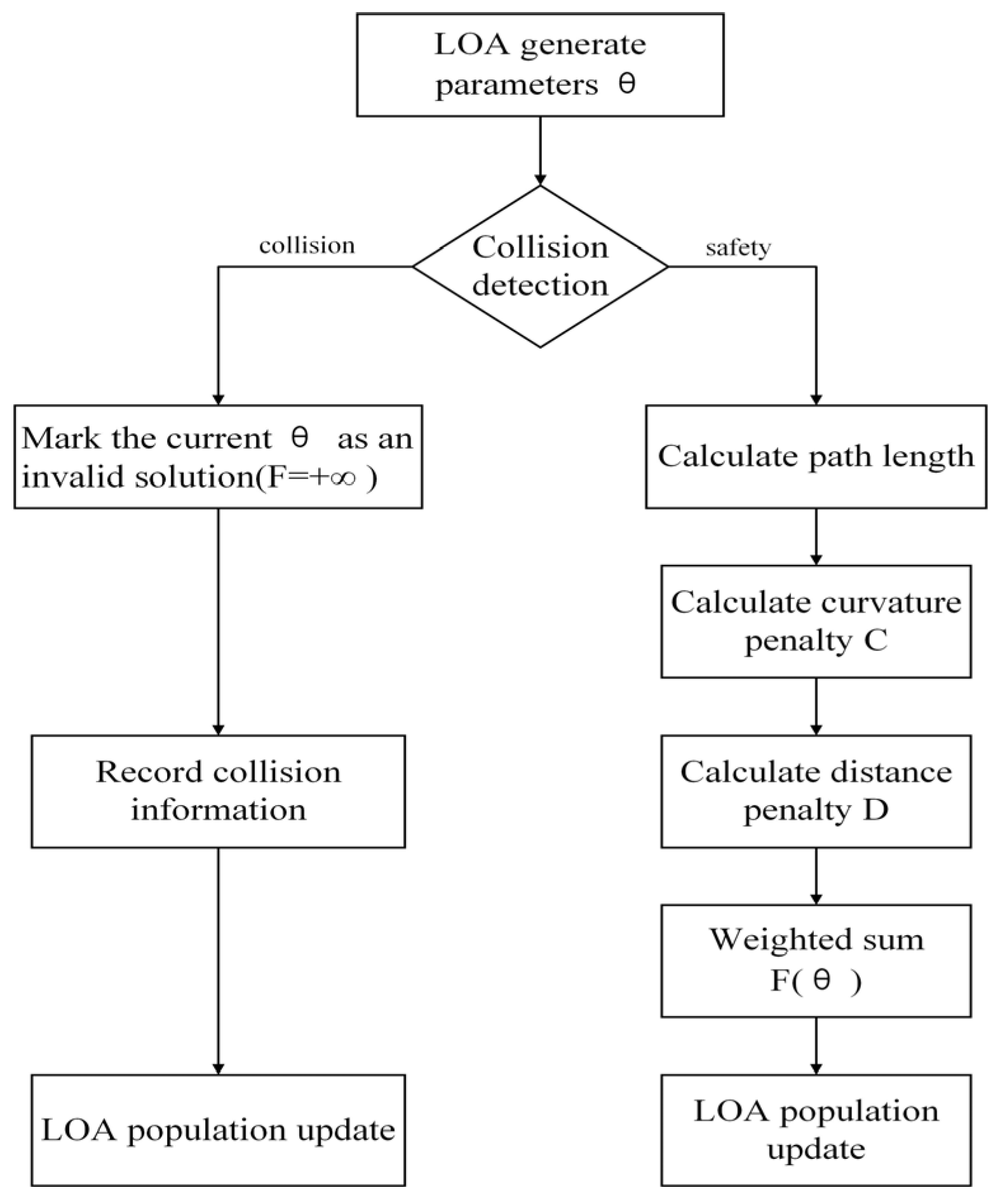
4.2.1. Objective Function (Fitness Function)

The objective function is used to evaluate the path quality, enabling the LOA to identify superior paths when optimizing the improved hybrid A* algorithm. This function typically incorporates multiple critical factors, such as the path length, smoothness, and safety (obstacle avoidance), as detailed in Equation (25):

$$f\left(\theta \right)=\left\{\begin{array}{ll}\hspace{1em}L(\theta )& Ifthepathisvalidandsafe\\ {\omega }_1\cdot \mathrm{L}+{\omega }_2\cdot C+{\omega }_3\cdot \mathrm{D}& Ifthepathisinvalidorcollides\end{array}\right.$$

(25)

where $\theta =\left[{\theta }_1,{\theta }_2,{\theta }_3\right]=\left[\min \_r,step,P_{\theta }\right]$ is the parameter vector to be optimized, and $L\left(x\right)$ is the path length; $C$ is the curvature penalty (smoothness); $D$ is the obstacle distance penalty (safety); and ); ${\omega }_1,{\omega }_2\mathrm{and}{\omega }_3$ are the weighting factors.

Each of these sub-items plays a different role in the algorithm, as shown in

Table 5. Roles of objective function parameters.

Parameter Name	Function
Path length	Normalizes the path length, encouraging the generation of shorter paths
Curvature penalty	Penalizes sharp turns to ensure that the path satisfies the vehicle’s kinematic constraints (for example, min_r)
Distance penalty	Ensures that the path is free of obstacles to improve the safety
Collision penalty	If the path collides with an obstacle, the system returns directly to +∞ and infeasible solutions are eliminated

.

In hybrid path planning algorithms, kinematic constraints play a crucial role in both the global search and local optimization stages, working together to ensure that the generated paths comply with the vehicle’s physical characteristics while meeting the actual driving requirements. The following is a stage-by-stage analysis of their importance and technical implementation.

(1)

Global search phase (exploring diversity)

The parameters are primarily constrained by their ranges, with upper and lower bounds (lb, ub) used to limit them. A minimum turning radius (min_r) ∈ [0.8, 1.2] is suitable for vehicle kinematics; the step size of the path search ∈ [0.4, 0.6] balances precision and computational efficiency; and the weight of the curvature penalty P_θ ∈ [0.005, 0.015]. Initial solutions are generated around the standard parameters following a normal distribution, balancing diversity and feasibility.

(2)

Local search phase (developing optimality)

Kinematics feasibility verification: Each time the hybrid A* algorithm is called, the isPathClear function is used to check whether the path meets the following conditions: minimum turning radius—the path curvature is constrained by min_r; continuous curvature—ensures path smoothness through the curvature penalty term C. Post-processing optimization (path post-processing) further smooths the path while checking the kinematic constraints. During multiple optimization attempts (num_trials), the system dynamically narrows the parameter range (e.g., lb_trial, ub_trial) to focus on a more optimal solution space.

4.2.2. Penalty Function

In the hybrid path algorithm system, the penalty function is mainly reflected in the fitness function through multi-objective weighting. It is the core constraint processing mechanism of the LOA and hybrid A* fusion, ensuring the feasibility and quality of the path through hard constraints (collision) and soft constraints (curvature, distance), as shown in the following Equation (26):

$$F(\theta )={\omega }_1\cdot {\displaystyle \frac{L(\theta )}{L_{ref}}}+{\omega }_2\cdot \max \left|\kappa (\theta )\right|+{\omega }_3{\displaystyle \sum _{k=1}^N{e}^{-d_k/\sigma }}+P_{hard}$$

(26)

where $\theta =\left[{\theta }_1,{\theta }_2,{\theta }_3\right]=\left[\min \_r,step,P_{\theta }\right]$ as the hybrid A* parameters to be optimized; $L\left(\theta \right)$ is the path length generated by hybrid A*; $L_{ref}$ is the standard parameter path length; $\kappa (\theta )$ is the curvature at each point along the path; $d_k$ is the distance from the kth point on the path to the nearest obstacle; $\sigma =0.5$ is the obstacle influence range parameter; $P_{hard}$ is the hard penalty (returns the maximum value at the point of collision); ${\omega }_1=0.6$ (path length weighting); ${\omega }_2=0.3$(curvature smoothing weight); ${\omega }_3=0.1$ (obstacle distance weighting). The workflow of the penalty function in the LOA is shown in Figure 8.

The penalty function achieves the collaborative optimization of global and local planning through a hierarchical penalty mechanism, where the penalty function of hybrid A* ensures the global feasibility of the path (such as obstacle avoidance constraints), while the LOA penalty function optimizes the local path quality (e.g., smoothness). By dynamically adjusting the adaptive penalty intensity of the safety distance, the multi-objective optimization problem is transformed into a mathematical expression of constraint conditions, thereby achieving a multi-dimensional balance of path safety, efficiency, and comfort at the algorithmic level.

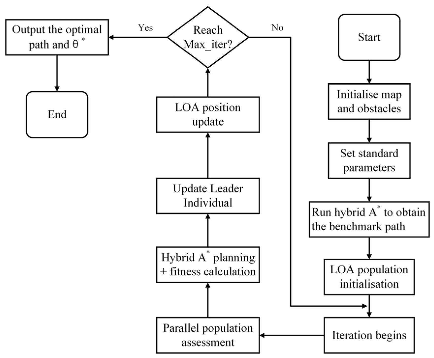
4.3. Fusion Algorithm Workflow

The core fusion mechanism of the system builds a closed-loop architecture of parameter generation–path planning–safety assessment–feedback optimization through the deep coupling of the LOA and the improved hybrid A* algorithm. The workflow is shown in Figure 9.

A multi-stage dynamic optimization strategy (including a parameter space refinement search and path post-processing optimization) is adopted to achieve dual coordination between global parameter optimization and local path optimization, ultimately forming an intelligent path planning system that is adaptive to environmental constraints.

5. Simulation Experiments

5.1. Map Construction

In order to verify the effectiveness and superiority of the improved hybrid A* algorithm based on the LOA, this study employed MATLAB R2023b as the simulation platform, and the LOA, sine cosine algorithm (SCA), and grey wolf optimizer (GWO) were used to perform simulations in a map environment.

This study constructed two different types of grid maps (complex scenario and simple scenario), as shown in Figure 10, where both maps have dimensions of 10 × 10 (scaled proportionally). The pentagram in the bottom-left corner served as the starting point (0.3, 0.4); the green circle in the top-right corner was the target point (9.3, 9.4); black squares represent obstacle zones, while white grids indicate obstacle-free zones. The obstacle coverage rate in the simple scenario was 9%, while that in the complex scenario was 18%.

5.2. Selection of Algorithm Parameters

The parameter settings of an optimization algorithm directly affect its convergence, accuracy, and robustness. The key parameters need to be finely tuned: a population size that is too small will reduce the search capabilities, while one that is too large will increase the computational burden. Adaptive mechanisms can dynamically optimize the parameters to enhance the algorithm’s adaptability. Parameter tuning should be tailored to the problem characteristics and achieved through experiments or automated tools to optimize the performance. The key parameters of the LOA are shown in

Table 6. Convergence control parameters.

Parameter/Variable	Function	Expression Value
Max_iter	Maximum number of iterations	Set by yourself (40)
progress	Iteration progress	Iter/Max_iter
theta	Exploration angle adjustment	2 × atan(1 − progress0.8)
No_improve_count	Early stop counter	Threshold(10)
E	Exploration–exploitation Switching threshold	2 × log(1/(rand() + 1 × 10−10)) × theta
N	Population size	25

.

The role of convergence control parameters is to dynamically adjust the search behavior of the algorithm, balancing global exploration (avoiding premature convergence) and local exploitation (rapidly approaching the optimal solution), as shown in

Table 7. Location update weight parameters.

Parameter	Function	Expression Value
Local_weight	Current optimal solution guidance weight	0.5 + 0.5 × progress
Learn_rate	Historical optimal learning rate	Max(0.2, 1 − progress)
Parameters	Function	Expression value
Spiral_coef	Spiral search coefficient	1 − 0.5 × progress
G	Global jump strength	2 × (sign(rand−0.5)) × (1 − progress2)
global_mean	Population mean guidance	0.1 × rand
best_history	Historical optimal solution guidance	0.05

.

The role of position update weights is to dynamically adjust the direction and stride length of individual movements, balancing the algorithm’s global exploration capabilities and local exploitation accuracy. These weights directly influence how the population converges towards the optimal solution.

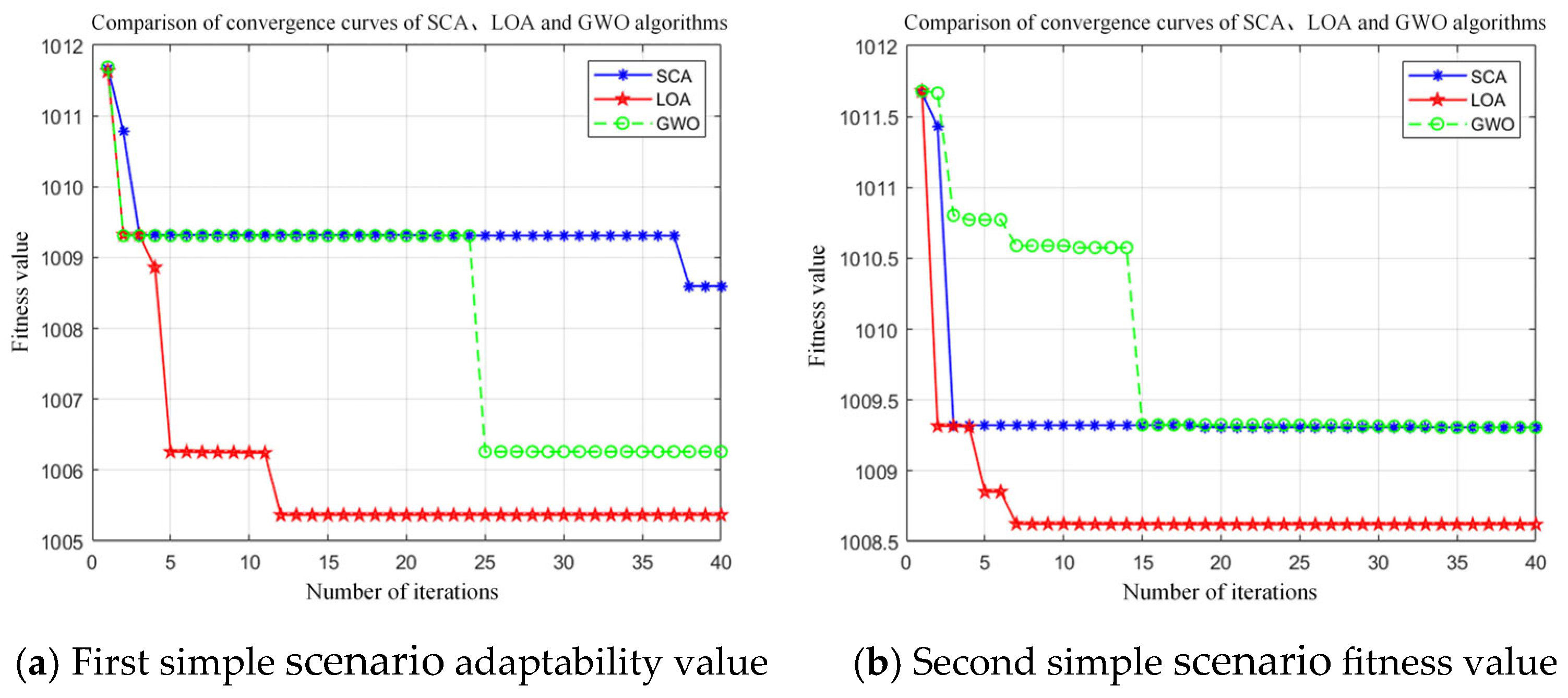
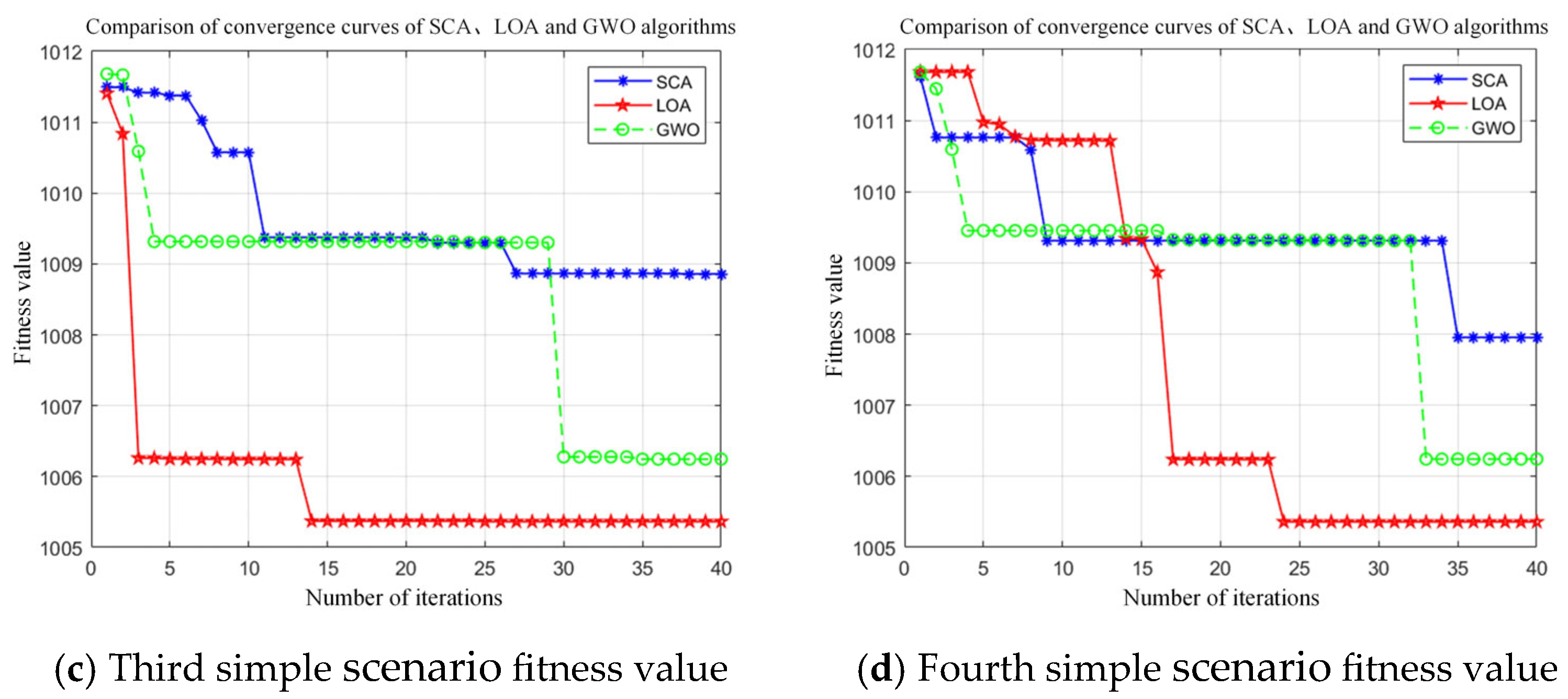
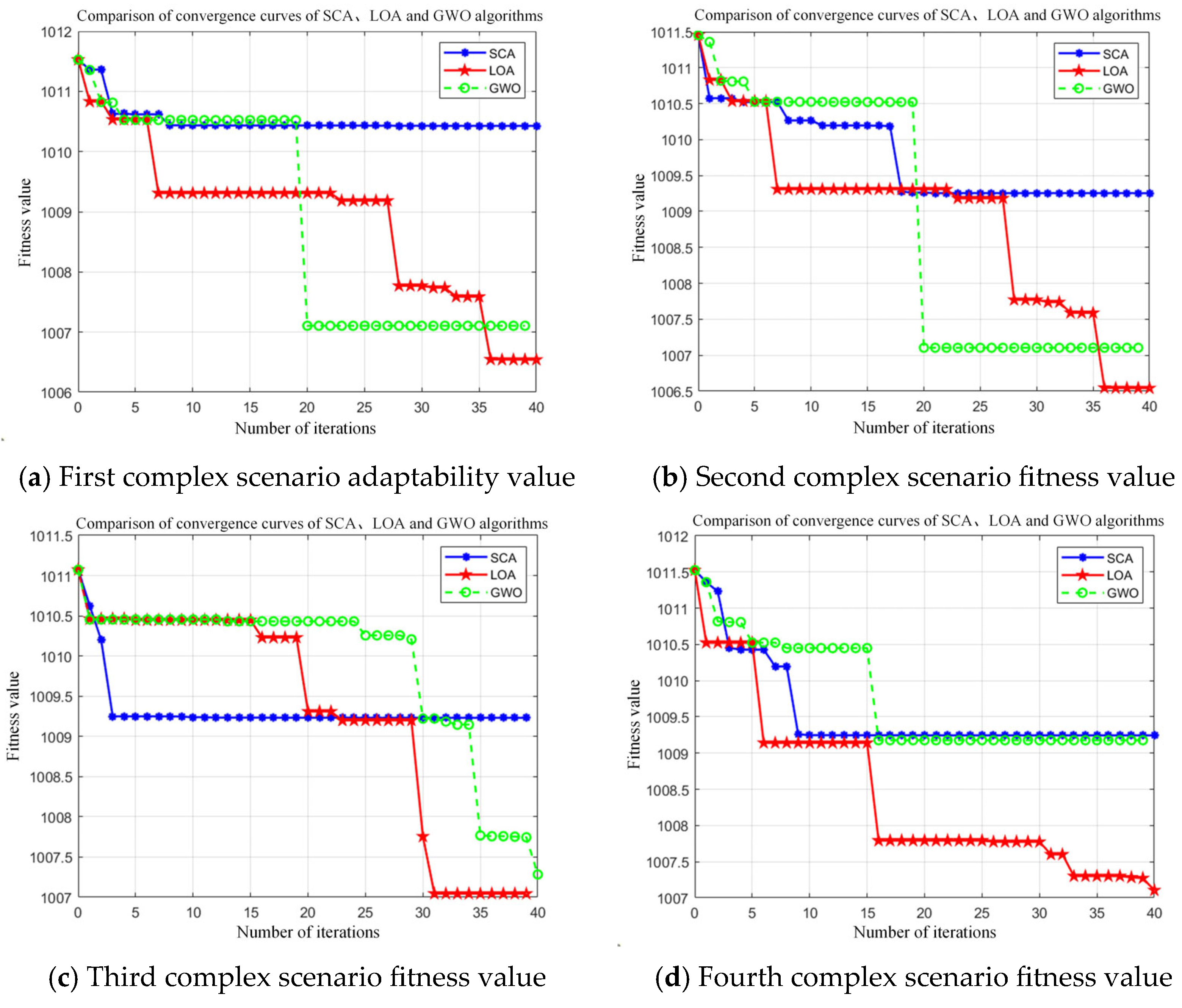
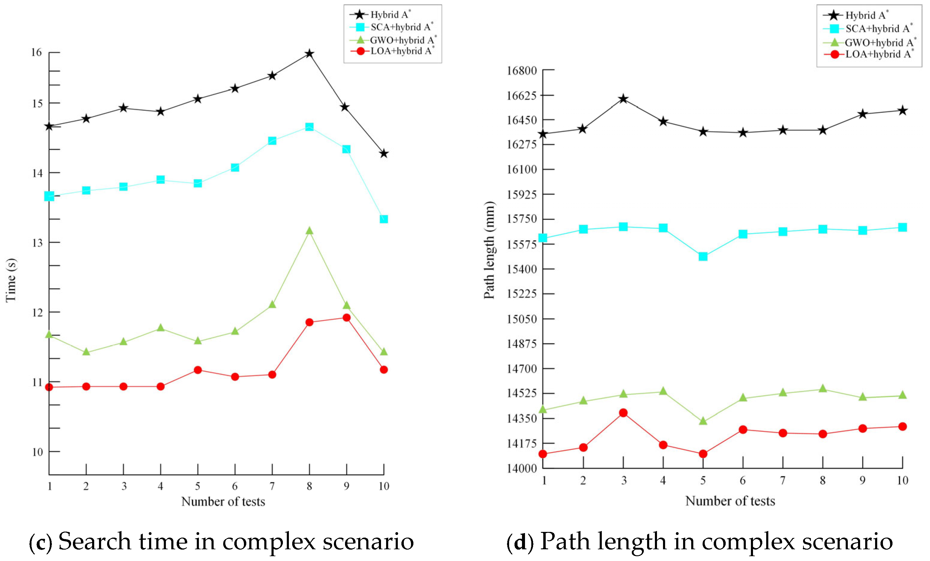
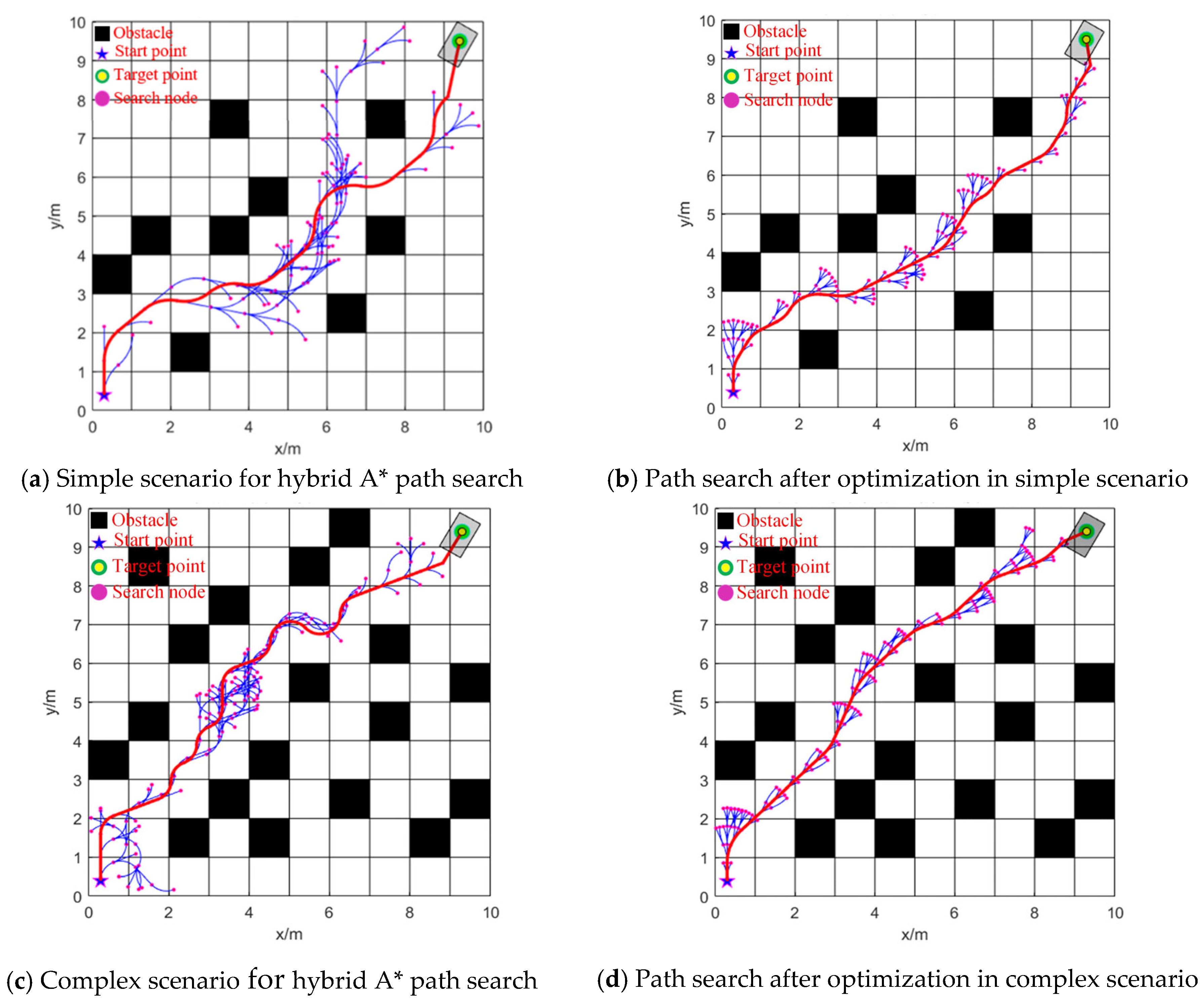
5.3. Simulation Result Analysis

By comparing the multiple evaluation metrics involved in the comprehensive fitness function (including the path length, smoothness, and obstacle avoidance safety), a smaller fitness value indicates better overall path performance. To ensure the broad applicability and reliability of the experimental results, multiple repeated experiments were conducted in both simple and complex scenarios to thoroughly compare and analyze the average performance of the algorithm. The method of multiple repeated experiments not only helps to reduce random errors in a single experiment but also more accurately reflects the general performance of the algorithm. The experimental results are shown in Figure 11 and Figure 12 and

Table 8. Comparison chart of algorithm convergence for simple scenario.

Optimization Algorithm	LOA Fitness Value	SCA Fitness Value	GWO Fitness Value
Number of tests 1	1,008.63	1,009.30	1,009.00
Number of tests 2	1,008.58	1,009.31	1,009.01
Number of tests 3	1,008.59	1,009.38	1,009.31
Number of tests 4	1,008.62	1,009.34	1,009.31
Number of tests 5	1,006.26	1,008.59	1,006.27
Number of tests 6	1,006.24	1,009.02	1,008.59
Number of tests 7	1,006.29	1,009.30	1,008.65
Number of tests 8	1,006.25	1,008.60	1,007.96
Number of tests 9	1,005.37	1,008.60	1,006.28
Number of tests 10	1,005.36	1,008.85	1,006.25
Average optimal fitness value	1,007.02	1,009.09	1,008.06

and

Table 9. Comparison chart of algorithm convergence for complex scenario.

Optimization Algorithm	LOA Fitness Value	SCA Fitness Value	GWO Fitness Value
Number of tests 1	1,007.22	1,010.42	1,009.24
Number of tests 2	1,005.68	1,010.43	1,007.06
Number of tests 3	1,007.59	1,010.43	1,009.24
Number of tests 4	1,006.54	1,010.43	1,007.24
Number of tests 5	1,007.07	1,011.35	1,009.24
Number of tests 6	1,006.54	1,010.43	1,007.72
Number of tests 7	1,007.07	1,009.25	1,007.07
Number of tests 8	1,006.55	1,009.23	1,007.26
Number of tests 9	1,007.07	1,010.43	1,009.25
Number of tests 10	1,006.55	1,009.24	1,007.25
Average optimal fitness value	1,006.79	1,010.14	1,008.06

.

The repeated experimental results indicate that, under the same number of iterations, the LOA algorithm achieved a final average best fitness value of 1,007.02, while the SCA and GWO algorithms yielded values of 1,009.09 and 1,008.06, respectively. Therefore, the overall simulation experiments demonstrate that the LOA exhibits superior local exploitation capabilities and optimization efficiency, delivering the best comprehensive optimization performance in this test. GWO ranks second, while SCA shows relatively poor effectiveness. The comparison of several algorithms in terms of path search parameters is shown in Figure 13 and

Table 10. Path performance metric comparison.

Scenario	Algorithm	Path Length/mm	Planning Time/s	Number of Nodes
Simple scenario	Hybrid A*	15,730.5	7.39	1150
	SCA + Hybrid A*	14,422.9	6.74	840
	GWO + Hybrid A*	14,175.6	6.38	820
	LOA + Hybrid A*	13,980.6	4.93	800
Complex scenario	Hybrid A*	16,421.2	14.79	1650
	SCA + Hybrid A*	15,700.0	14.01	1580
	GWO + Hybrid A*	14,433.5	11.86	1260
	LOA + Hybrid A*	14,188.2	11.31	1260

, and the comparison of path trajectories before and after optimization is shown in Figure 14.

As shown in Table 10, the traditional hybrid A* algorithm has the highest average planning time and average path length values in both the simple and complex scenarios, with average times of 7.39 s and 14.79 s and average lengths of 15,730.5 mm and 16,421.2 mm. This is because the traditional hybrid A* algorithm has high computational complexity and poor real-time performance.

Next, for the SCA optimization algorithm, in the simple scenario, the average planning time was 6.74 s and the average path length was 14,422.9 mm. Compared with the traditional hybrid A* algorithm, the average search time was reduced by 8.7% and the average path length was reduced by 8.3%. Meanwhile, in the complex scenario, the average planning time was 14.01 s and the average path length was 15,700.0 mm. Compared with the traditional hybrid A* algorithm, the average search time was reduced by 8.7% and the average path length was reduced by 8.3%.

For the GWO optimization algorithm, in the simple scenario, the average planning time was 6.38 s and the average path length was 14,175.6 mm. Compared with the traditional hybrid A* algorithm, the average search time was reduced by 13.6% and the average path length was reduced by 9.8%. Meanwhile, in the complex scenario, the average planning time was 11.86 s, and the average path length was 14,433.5 mm. Compared with the traditional hybrid A* algorithm, the average search time was reduced by 19.8% and the average path length was reduced by 12.1%.

Finally, for the LOA, in the simple scenario, the average planning time was 4.93 s, and the average path length was 13,980.6 mm. Compared with the traditional hybrid A* algorithm, the average search time was reduced by 33.2% and the average path length was reduced by 11.1%. Meanwhile, in the complex scenario, the average planning time was 11.31 s, and the average path length was 14,188.2 mm. Compared with the traditional hybrid A* algorithm, the average search time was reduced by 23.5% and the average path length was reduced by 13.6%.

Based on the overall simulation results, the improved hybrid A* algorithm based on lemming optimization demonstrates more efficient path searching and smoother path curves.

The simulations show that, in different scenarios and processes, there are some parameters that need to be adjusted numerically according to the scenario’s conditions in order to make the algorithm more stable, as shown in

Table 11. Comparison of LOA parameters in different scenarios.

Parameter	Suitable Value for Simple Scenario	Suitable Value for Complex Scenario	Adjustment Logic
Population size (N)	Minimum value (10–20)	Maximum value (20–30)	Complex scenarios require more diverse exploration.
Maximum number of iterations ()	Minimum value (20–30)	Maximum value (40–60)	Complex scenarios require longer convergence times.
Lévy flight intensity	Lower value (levy_strength = 0.1)	Higher value (levy_strength = 0.3)	Complex scenarios require stronger global leap capabilities.
Local search weight	Higher value (local_weight = 0.8)	Lower value (local_weight = 0.5)	Simple scenarios converge quickly, while complex scenarios require balance.

.

By comparing simple and complex scenarios and adjusting the parameters accordingly, it is found that the algorithm can balance efficiency and robustness in different scenarios. In practical applications, it is recommended to first use a grid search to determine the parameter range and then fine tune it using an optimization algorithm.

6. Conclusions

This paper proposes an improved hybrid A* algorithm with lemming optimization for autonomous vehicle path planning, incorporating the LOA to enhance the safety, smoothness, and search efficiency in trajectory generation. By integrating a penalty-based graph search with Reeds–Shepp curves, the proposed algorithm obtains collision-free paths with continuous curvature while maintaining a safe distance from obstacles. Furthermore, it effectively balances the global optimization capabilities of the LOA with the motion-aware local search of the improved hybrid A* algorithm to avoid local optima traps. The simulation results show that, in simple and complex scenarios, the improved hybrid A* algorithm can shorten the time by 33.2% and 23.5% and the path length by 11.1% and 13.6%, respectively, compared with the traditional hybrid A* algorithm. These findings confirm that the proposed approach excels in solving target path planning problems, combining rapid convergence with high-quality path generation, and exhibits strong potential for real-world applications.

Although the proposed lemming-optimized hybrid A* algorithm demonstrates significant improvements in safety, smoothness, and search efficiency, there remains room for enhancement, with several promising research directions.

(1) Although this method can reduce unnecessary searches on the path and shorten the search time, the proposed algorithm does not significantly improve the path length. Therefore, in future work, we will adjust the evaluation criteria to improve their suitability and introduce stricter penalty mechanisms to prevent the generation of excessively long paths.

(2) The current study assumes a static environment, which does not align with the real world. Therefore, in future work, the framework could be extended through online parameter adjustments to handle real-time dynamic obstacles and uncertain road conditions, enabling dynamic obstacle avoidance.

References

1. Song, F.Y. Driverless cars and their development. China High New Technol. 2019, 24–27. [Google Scholar] [CrossRef]
2. Yuan, S.Z.; Li, J. Summary of Research on Path Planning of Driverless Vehicles. Auto Eng. 2019, 5, 11–13. [Google Scholar]
3. Zhu, D.Q.; Yan, M.Z. A Review of Mobile Robot Path Planning Techniques. J. Control Decis. 2010, 25, 961–967. [Google Scholar] [CrossRef]
4. Teng, S.; Hu, X.; Deng, P.; Li, B.; Li, Y.; Ai, Y.; Yang, D.; Li, L.; Xuanyuan, Z.; Zhu, F.; et al. Motion planning for autonomous driving: The state of the art and future perspectives. IEEE Trans. Intell. Veh. 2023, 8, 3692–3711. [Google Scholar] [CrossRef]
5. Zhou, S.; Wang, R.Y.; Zhang, Y.F.; Zhang, G. Autonomous Vehicle Trajectory Generation Based on Hybrid A* Algorithm. Automot. Dig. 2023, 44–54. [Google Scholar] [CrossRef]
6. Dijkstra, E.W. A note on two problems in connexion with graphs. In Edsger Wybe Dijkstra: His Life, Work, and Legacy; Association for Computing Machinery: New York, NY, USA, 2022. [Google Scholar]
7. Marchese, F.M. Multiple mobile robots path-planning with MCA. In Proceedings of the International Conference on Autonomic and Autonomous Systems (ICAS), Silicon Valley, CA, USA, 19–21 July 2006. [Google Scholar]
8. Zhu, D.-D.; Sun, J.-Q. A new algorithm based on Dijkstra for vehicle path planning considering intersection attribute. IEEE Access 2021, 9, 19761–19775. [Google Scholar]
9. Sang, W.; Lin, M. Research on AGV path planning integrating an improved A* algorithm and DWA algorithm. Appl. Sci. 2024, 14, 7551. [Google Scholar]
10. Zhou, H.; Shang, T.; Wang, Y.; Zuo, L. Salp Swarm Algorithm Optimized A* Algorithm and Improved B-Spline Interpolation in Path Planning. Appl. Sci. 2025, 15, 5583. [Google Scholar]
11. Shim, T.; Adireddy, G.; Yuan, H. Autonomous vehicle collision avoidance system using path planning and model predictive control based active front steering and wheel torque control. Proc. Inst. Mech. Eng. Part D J. Automob. Eng. 2012, 226, 767–778. [Google Scholar]
12. Taghavifar, H. Optimal reinforcement learning and probabilistic-risk-based path planning and following of autonomous vehicles with obstacle avoidance. Proc. Inst. Mech. Eng. Part D J. Automob. Eng. 2024, 238, 1427–1439. [Google Scholar]
13. Reda, M.; Onsy, A.; Haikal, A.Y.; Ghanbari, A. Path planning algorithms in the autonomous driving system: A comprehensive review. Robot. Auton. Syst. 2024, 174, 104630. [Google Scholar]
14. Zhu, S. Obstacle-Avoidance path planning of unmanned vehicles based on polynomial optimization. In Proceedings of the 2022 China Automation Congress (CAC), Xiamen, China, 25–27 November 2022; pp. 6988–6992. [Google Scholar]
15. Zhou, W.; Li, J. Research on obstacle avoidance path planning of automatic driving vehicle. Auto Eng. 2018, 55–58. Available online: https://www.sohu.com/a/239903213_99949100 (accessed on 4 July 2025).
16. Li, X.C. Smooth and collision-free trajectory generation in cluttered environments using cubic B-spline. Mech. Mach. Theory 2022, 169, 104606. [Google Scholar]
17. Zheng, L.; Zeng, P.; Yang, W.; Li, Y.; Zhan, Z. Bézier curve-based trajectory planning for autonomous vehicles with collision avoidance. IET Intell. Transp. Syst. 2020, 14, 1882–1891. [Google Scholar]
18. Zhu, Y.J.; Li, J.S.; Fen, M.Y.; Xu, Y.C. Autonomous parking path planning algorithm for intelligent vehicles based on numerical optimization. J. Mil. Transp. 2019, 21, 84–89. [Google Scholar]
19. Hu, C.; Zhao, L.; Qu, G. Event-Triggered model predictive adaptive dynamic programming for road intersection path planning of unmanned ground vehicle. IEEE Trans. Veh. Technol. 2021, 70, 11228–11243. [Google Scholar]
20. Ji, J.; Khajepour, A.; Melek, W.W.; Huang, Y. Path planning and tracking for vehicle collision avoidance based on model predictive control with mult constraints. IEEE Trans. Veh. Technol. 2016, 66, 952–964. [Google Scholar]
21. Li, Y.; Liu, Y. Research on Path Planning Based on the Integrated Artificial Potential Field-Ant Colony Algorithm. Appl. Sci. 2025, 15, 4522. [Google Scholar]
22. Bojarski, M.; Del Testa, D.; Dworakowski, D.; Firner, B.; Flepp, B.; Goyal, P.; Jackel, L.D.; Monfort, M.; Muller, U.; Zhang, J.; et al. End to end learning for self-driving cars. Comput. Sci. 2022. [Google Scholar] [CrossRef]
23. Wang, Y.; Wang, S.; Chao, T. Autonomous vehicle path planning algorithm based on improved Q-learning. In International Conference on Guidance, Navigation and Control; Springer Nature: Singapore, 2024. [Google Scholar]
24. Zhang, L.; Zhang, Y.; Li, Y. Path planning for indoor mobile robot based on deep learning. Optik 2020, 219, 165096. [Google Scholar]
25. Chen, L.; Wu, P.; Chitta, K.; Jaeger, B.; Geiger, A.; Li, H. End-to-end autonomous driving: Challenges and frontiers. IEEE Trans. Pattern Anal. Mach. Intell. 2024, 46, 10164–10183. [Google Scholar] [PubMed]
26. Rodríguez, N.; Gupta, A.; Zabala, P.L.; Cabrera-Guerrero, G. Optimization algorithms combining (meta) heuristics and mathematical programming and its application in engineering. Math. Probl. Eng. 2018. [Google Scholar] [CrossRef]
27. Bu, Z.; Korf, R.E. A*+ BFHS: A hybrid heuristic search algorithm. Proc. AAAI Conf. Artif. Intell. 2022, 36, 10138–10145. [Google Scholar]
28. Hoel, C.J.; Driggs-Campbell, K.; Wolff, K.; Laine, L.; Kochenderfer, M.J. Combining planning and deep reinforcement learning in tactical decision making for autonomous driving. IEEE Trans. Intell. Veh. 2019, 5, 294–305. [Google Scholar]
29. Nielsen, I.; Bocewicz, G.; Saha, S. Multi-agent path planning problem under a multi-objective optimization framework. In Distributed Computing and Artificial Intelligence, Special Sessions, 17th International Conference, L’Aquila, Italy, 17–19 June 2020; Springer International Publishing: Cham, Switzerland, 2021; pp. 5–14. [Google Scholar]
30. Badue, C.; Guidolini, R.; Carneiro, R.V.; Azevedo, P.; Cardoso, V.B.; Forechi, A.; Jesus, L.; Berriel, R.; Paixao, T.M.; Mutz, F.; et al. Self-driving cars: A survey. Expert Syst. Appl. 2021, 165, 113816. [Google Scholar]
31. Hu, J.; Wu, H.; Zhong, B.; Xiao, R. Swarm intelligence-based optimization algorithms: An overview and future research issues. Int. J. Autom. Control 2020, 14, 656–693. [Google Scholar]
32. Xiao, Y.; Cui, H.; Abu Khurma, R.; Castillo, P.A. Artificial lemming algorithm: A novel bionic meta-heuristic technique for solving real-world engineering optimization problems. Artif. Intell. Rev. 2025, 58, 84. [Google Scholar]
Figure 1. Flowchart of LOA and hybrid A* algorithm fusion.
Applsci 15 07734 g001
Figure 2. Hybrid A* search method.
Applsci 15 07734 g002
Figure 3. Schematic diagram of the 2D long-distance migration model.
Applsci 15 07734 g003
Figure 4. Schematic diagram of 2D digging model.
Applsci 15 07734 g004
Figure 5. Schematic of the 2D foraging model.
Applsci 15 07734 g005
Figure 6. Schematic of the 2D predator avoidance model.
Applsci 15 07734 g006
Figure 7. Schematic diagram of the improved distance heuristic function.
Applsci 15 07734 g007
Figure 8. Workflow diagram of penalty function in LOA.
Applsci 15 07734 g008
Figure 9. Workflow diagram of fusion algorithm.
Applsci 15 07734 g009
Figure 10. Map environment.
Applsci 15 07734 g010
Figure 11. Comparison of convergence curves for simple scenario.
Applsci 15 07734 g011aApplsci 15 07734 g011b
Figure 12. Comparison of convergence curves for complex scenario.
Applsci 15 07734 g012
Figure 13. Comparison of path search parameters.
Applsci 15 07734 g013aApplsci 15 07734 g013b
Figure 14. Comparison of path search before and after optimization.
Applsci 15 07734 g014