Intelligent System Using Data to Support Decision-Making

Abstract

Interest in explainable machine learning has grown, particularly in healthcare, where transparency and trust are essential. We developed a semi-automated evaluation framework within a clinical decision support system (CDSS-EQCM) that integrates LIME and SHAP explanations with multi-criteria decision-making (TOPSIS and Borda count) to rank model interpretability. After two-phase preprocessing of 2934 COVID-19 patient records spanning four epidemic waves, we applied five classifiers (Random Forest, Decision Tree, Logistic Regression, k-NN, SVM). Five infectious disease physicians used a Streamlit interface to generate patient-specific explanations and rate models on accuracy, separability, stability, response time, understandability, and user experience. Random Forest combined with SHAP consistently achieved the highest rankings in Borda count. Clinicians reported reduced evaluation time, enhanced explanation clarity, and increased confidence in model outputs. These results demonstrate that CDSS-EQCM can effectively streamline interpretability assessment and support clinician decision-making in medical diagnostics. Future work will focus on deeper electronic medical record integration and interactive parameter tuning to further enhance real-time diagnostic support.

1. Introduction

There has been a growing interest in topics related to the explanation, interpretation, and understanding of ML models in recent years. This problem is becoming more and more attractive and has been addressed in several studies. Physicians strive to make the best possible decisions when making diagnoses, designing treatments, preventing diseases, or drawing conclusions. They are continually looking for new solutions to improve and confirm their decisions with confidential systems. Therefore, it is necessary to support medical decision-making regarding the analysis and prediction of a patient’s condition, whether in treatment or diagnosis. The completeness and timeliness of the available patient information are essential when making decisions. To facilitate, speed up and streamline medical decisions, intelligent devices, intelligent systems, and methods are often integrated into the medical field.

Clinical Decision Support Systems (CDSS) are essential in modern healthcare, where clinicians must fuse heterogeneous data—such as demographics, laboratory and imaging results, comorbidities, and real-time monitoring—to make timely, high-stakes decisions [1,2]. These systems must balance multiple, often conflicting criteria (e.g., diagnostic accuracy, treatment efficacy, risk minimization, workflow efficiency), which compounds their complexity and necessitates transparent reasoning via multi-criteria decision-making frameworks. Without clear interpretability and explainability, “black-box” recommendations can undermine clinician trust, impede adoption, and obscure how trade-offs are managed [3,4]. By integrating model-agnostic explanation techniques (e.g., LIME, SHAP) with quantified metrics of separability, stability, and user experience, CDSS can reveal why specific predictions or rankings were made and how input variations affect outcomes. Such transparency not only strengthens clinical confidence and facilitates second-opinion workflows but also ensures that multi-criteria decisions remain evidence-based and auditable [5,6].

Recent efforts have begun to integrate explainable AI (XAI) with multi-criteria decision-making (MCDM), often grounded in axiomatic frameworks that ensure fairness, consistency, and rationality. Axiomatic analyses of preference-aggregation methods (e.g., properties of TOPSIS and Borda count;) [7] and of explanation-quality metrics (identity, stability, separability) provide formal guarantees for both model ranking and interpretability. In the transportation domain, Eun Hak Lee et al. recently proposed an “eXplainable DEA” approach to evaluate public-transport origin–destination efficiency, coupling Data Envelopment Analysis with SHAP-based local explanations to reveal how input factors drive efficiency scores [8]. Building on this, the same group developed an Iterative DEA (iDEA) framework for transfer-efficiency assessment in super-aging societies; iDEA alternates between DEA efficiency estimation and stakeholder-guided adjustment of input–output weights, yielding both robust performance rankings and transparent, context-sensitive insights [8]. These methodologies exemplify how axiomatic MCDM and XAI can be combined to produce decision-support tools that are not only accurate and fair but also interpretable and directly actionable by domain experts.

Currently, when solving the issue of explainability, we meet several terms such as explainability and interpretability. In the XAI literature, interpretability and explainability are distinct concepts [9,10]. We follow Doshi-Velez and Kim [9] in defining interpretability as an intrinsic property of a model—its internal logic (e.g., decision rules or coefficients) can be directly understood without auxiliary tools. By contrast, explainability refers to post hoc analyses that attach human-readable justifications to a model’s output, even when the model itself is a black box (e.g., deep nets or Random Forests). Interpretability is the ability of a model to be easy to understand from its very essence—that is, without additional tools or explanations. Interpretability means that the model is understandable just by looking at it. Explainability refers to the model’s ability to explain why it made the decisions it made. In other words, explainability answers the question: “Why did this model make a particular prediction?”. Explainability focuses on the creation of additional tools (e.g., LIME, SHAP, Partial Dependence Plots) that help users understand the logic of the decision, even if the model itself is complex and non-transparent (“black box”) [6]. In this work, we train two inherently interpretable models (Decision Tree, Logistic Regression) and three black-box models (Random Forest, k-NN, SVM). Because clinicians found the raw tree diagrams and coefficient tables difficult to parse, we also applied LIME and SHAP to the Decision Tree and Logistic Regression, ensuring that every model—interpretable or black box—produces intuitive, visual explanations. Throughout, we reserve interpretability for models whose structure and parameters admit direct human understanding, and explainability for algorithmic routines that generate post hoc insights into any classifier’s behavior. Whenever clinicians require more digestible visuals, we employ explainability methods (LIME, SHAP) even on interpretable models.

In medical applications, achieving high prediction accuracy is often as crucial as understanding the prediction [11]. Gilpin et al. [12] describe the primary goal of explainability as the ability to explain the ins and outs of the system in an understandable way to end users. We can understand an explainable model, and it is related to accuracy, efficiency, and explainability. In addition, interpretability is often associated with a new wave of ML research. In this case, it provides confidence in the ML system’s development process for end users of such systems [13]. The explanation of ML models is often driven by different motivations, such as explainability requirements, the impact of high-risk decision-making, societal concerns, and ML requirements, regulations, and others. There are already several different definitions for the term explainability. However, we will follow the opinion of Miller [6] and Molnar [10], i.e., that explainability (in the context of AI and ML) refers to the ability of a model or algorithm to provide a clear and understandable explanation of how it arrived at its decisions or predictions. The goal is to remove the need for users (such as analysts, targets, or end users) to understand why the model performed a particular need or provided a particular output.

If we talk about interpretable explanations of individual models, several methods exist to interpret the result in a comprehensible and trustworthy way. They point out why the model decided in this way and what led it to do so. Without robust explainability techniques, it would not be easy to understand these decisions. In our work, we considered the following methods: Local Interpretable Model-Agnostic Explanations (LIME) and SHapley Additive ExPlanations (SHAPs).

Understanding the reasons for predictions, causes and recommendations is essential for several reasons. One of the most important reasons is the trustworthiness of the result [14]. Moreover, the next area that needs to be considered is the direct measurement of the user’s perception of the utility of the explanations, including the causal considerations, using a good usability approach. Then, it follows by measuring the user experience, i.e., the usability of the software products [15]. Efficiency, effectiveness, and user satisfaction need to be considered when measuring interface usability. Holzinger et al. 2019 [16] propose the notion of causability as the degree to which an explanation to a human expert reaches a specified level of causal understanding with effectiveness, efficiency, and satisfaction in a specified context of use. In other words, causability is a person’s ability to understand the explanations of ML models. Subsequently, Holzinger et al. 2020 [5] were the first to focus on measuring the quality of individual explanations or interpretable models and propose a system causability scale (SCS) metric in combination with concepts adapted from a generally accepted usability scale.

Based on many years of cooperation with physicians and several joint research projects, where we constantly generated a variety of models and visualizations, we found that understanding all the models is time-consuming for physicians. Therefore, we proposed an evaluation mechanism based on multi-criteria decision-making combining various metrics for the explainability of decision models. The TOPSIS method and the Borda method determined which created model is the best from the point of view of the preferences of the target user. Also, transparent explanations of how the algorithms arrive at their prediction through the explainable methods LIME and SHAP will be available. By providing transparent interpretations of prediction models, we can build confidence in the predictions and increase the likelihood of the algorithm being adopted in clinical practice. The results generated can help understand the factors that influence prediction.

Related Work

Itani et al. [17] propose an expert-in-the-loop methodology for ADHD prediction that iteratively refines Decision Trees to balance accuracy and interpretability. Starting with an automatically generated tree, medical experts review and adjust its structure; the final model achieved 73.2% test accuracy, demonstrating that incorporating domain knowledge can yield more meaningful decision rules without severely sacrificing performance. Ribeiro et al. [3] introduce LIME, a model-agnostic explanation technique validated on text (SVM, RF, LR, DT) and image (deep networks) classifiers. Through simulated user studies, they show that LIME explanations increase both expert and non-expert trust and understanding across diverse tasks, underlining its utility for verifying model behavior and fostering confidence in predictions. Wu et al. [18] analyze four ML algorithms (DT, RF, GBT, NN) on early COVID-19 patient data and apply PDP, ICE, ALE, LIME, and SHAP to identify key biomarkers of disease severity. Local explanations from SHAP and LIME were rated by physicians, and all models matched expert diagnoses. Similarly, study [19] evaluates LIME outputs on a 13,713-record sepsis dataset using AdaBoost, RF, and SVM; RF (ntree = 300) achieved top performance, and clinicians preferred graphical over textual explanations (4.3/5). Thimoteo et al. [20] apply LR, RF, and SVM to 5647 Brazilian COVID-19 cases, prioritizing F₂ to capture true positives; SHAP interpretations for RF and SVM enhanced both local and global transparency. Nesaragi et al. [21] develop xMLEPS—an explainable LightGBM ensemble—for early ICU sepsis prediction, employing ten-fold validation and SHAP plots to elucidate physiological relationships and ensure clinical generalizability. Prinzi et al. [22] integrate clinical, laboratory, and chest X-ray radiomic features (1589 patients) using RF and SVM within a multi-level explainability framework: global feature importance and local patient-specific rationales. Gabbay et al. [23] combine MLP and DT models with LIME to predict COVID-19 severity, achieving up to 80% accuracy and providing individualized condition insights via a mobile application for medical staff. Study [24] benchmarks six interpretability methods (LIME, SHAP, Anchors, ILIME, LORE, MAPLE) on RF models across identity, stability, separability, runtime, bias detection, and confidence metrics, finding no universal best. Yasodahara et al. [14] compare SHAP and gain-based importances for tree ensembles, reporting slightly higher stability for SHAP under noisy inputs. Several works address deep hierarchies in Sunburst visualizations. The authors of [25] develop three extensions to reveal lower levels in complex trees; Liu and Wang [26] propose the Necklace Sunburst, which interactively toggles deep layers; and Rouwendal van Schijndel et al. [27] demonstrate Sunburst’s clarity for crisis-management exercise planning.

2. Materials and Methods

Effective decision-making relies on high-quality information: each option is characterized by a set of attributes and evaluated against specific criteria [28]. In this work, we first derive criterion weights via quantitative pairwise comparisons using Saaty’s matrix. We then rank alternatives using two complementary multi-criteria methods: TOPSIS (Technique for Order Preference by Similarity to Ideal Solution), which orders options by their distance to an ideal (best) and anti-ideal (worst) solution, producing a full preference list [29,30], and Borda count, where voters assign points to each alternative based on its rank; the sum of points across all voters determines the final ordering [31]. Together, these approaches provide a robust, transparent framework for multi-criteria decision support.

In everyday life, we often face the need to make decisions, drawing on our experience and information from our surroundings. Decision-making is a key component of management, where individuals or groups aim to choose options that best match initial conditions and support goal achievement. The process involves selecting the most suitable alternative from available solutions, based on relevant, high-quality information. To evaluate these options, we assess objects according to specific criteria. Each decision-making scenario can thus be represented by a set of attribute values used in multi-criteria decision-making [28].

Theories of multi-criteria decision-making are based on mathematical modeling [29]. Several multi-criteria decision-making methods exist that share the same principle—evaluating multiple solution alternatives to a given problem according to selected criteria and establishing a ranking of these variants. These methods differ in how the weight of each criterion is determined and how the extent to which each alternative meets the chosen criteria is numerically assessed. One such method is multi-criteria evaluation of alternatives. The goal of multi-criteria evaluation is to objectively describe the reality of the selection process using standard procedures, thereby formalizing the decision problem—that is, converting it into a mathematical model of a multi-criteria decision-making situation.

The assessment criteria and methods for obtaining quantitative data on the values for the individual decision alternatives are determined. This is characterized by the so-called criteria matrix, see Equation (1), where the rows represent the alternatives, and the columns represent the criteria.

$$\begin{gathered} \begin{array}{ccc}{f}_1& f_2 & \begin{array}{cc}. & f_j\end{array}\end{array} \\ \begin{array}{c}{a}_1\\ a_2\\ \begin{array}{c}.\\ .\\ a_i\end{array}\end{array}\left[\begin{array}{ccc}\begin{array}{c}{y}_{11}\\ y_{21}\\ \begin{array}{c}.\\ .\\ y_{i1}\end{array}\end{array}& \begin{array}{c}{y}_{12}\\ y_{22}\\ \begin{array}{c}.\\ .\\ y_{i2}\end{array}\end{array}& \begin{array}{cc}\begin{array}{c}.\\ .\\ \begin{array}{c}.\\ .\\ .\end{array}\end{array}& \begin{array}{c}{y}_{1j}\\ y_{2j}\\ \begin{array}{c}.\\ .\\ y_{ii}\end{array}\end{array}\end{array}\end{array}\right] \end{gathered}$$

(1)

Columns = the selected criteria $(f_1, f, ...f_j)$ serve to select the most suitable alternative. Rows = alternatives considered $(a_1, a_2, ...a_i).$

In multi-criteria decision-making tasks, we will analyze two problems [30]:

• Modeling preferences among criteria—that is, determining the importance (weight) that individual criteria hold for the user.
• Modeling preferences among alternatives with respect to individual criteria and aggregating them to express the overall preference.

Modeling preference among criteria involves analyzing the importance (weight) that individual criteria have for the user. Preferences can be modeled using several approaches. The most used methods include

• the ranking method,
• the scoring method,
• the pairwise comparison method of criteria,
• the quantitative pairwise comparison method of criteria (Saaty’s method).

To solve our task, we selected the quantitative pairwise comparison method. When creating pairwise comparisons, we use a scale of 1, 3, 5, 7, 9, with the values interpreted as follows:

• 1—criteria $i$ and $j$ are of equal importance,
• 3—criterion $i$ is slightly preferred over $j$,
• 5—criterion $i$ is strongly preferred over $j$,
• 7—criterion $i$ is very strongly preferred over $j$,
• 9—criterion $i$ is absolutely preferred over $j.$

The values 2, 4, 6, and 8 represent intermediate levels. The elements of the matrix $s_{ij}$ are expressed as estimates of the ratio of the weights of the $i$-th criterion to the $j$-th criterion.

$$s_{ij}\approx {\displaystyle \frac{v_i}{v_j}} i,j=1, 2, 3, \dots \dots , k$$

(2)

Such a matrix is called the Saaty matrix, and its elements are

$$\begin{gathered} s_{ij }=1 i=1, 2, 3, \dots \dots k \\ {s}_{ij }={\displaystyle \raisebox{1ex}{$1$}\!\left/ \!\raisebox{-1ex}{$s_{ij }$}\right.} i, j=1, 2, 3, \dots \dots k \end{gathered}$$

(3)

The methods for modeling preferences among criteria are divided into three groups:

Methods with information on aspirational levels of criteria: the decision-maker (user) is required to provide at least the aspirational levels for the criteria values, i.e., the values that each alternative should at least achieve.

Methods with cardinal information about the criteria: the user is required to provide cardinal information regarding the relative importance of the criteria, which can be expressed using a vector of criteria weights.

Methods with cardinal information about the criteria: the user is required to provide cardinal information regarding the relative importance of the criteria, which can be expressed using a vector of criteria weights. This group of methods is the largest and primarily includes

• the maximum utility method,
• the method of minimizing the distance to the ideal alternative (Technique for Order Preference by Similarity to Ideal Solution—TOPSIS),
• the method of evaluating alternatives based on a preference relation.

For a complete ranking of the alternatives, we use the method of minimizing the distance to the ideal alternative, which requires the user to supply substantial information about the criteria. The most used method is TOPSIS.

TOPSIS is a multi-criteria decision-making method that ranks alternatives based on their distance from the ideal (best) and the basal (worst) solutions. It identifies the best option by selecting the alternative closest to the ideal and farthest from the worst. The method requires criterion values for each alternative, and the weights of each criterion. These values are organized in a decision matrix $Y=y_{ij}$, where $y_{ij}$ represents the value of the i-th alternative with respect to the j-th criterion. The method is based on selecting the alternative that is closest to the ideal alternative, represented by the vector $(H_1, H_2, H_3 ,\dots \dots H_k$) and farthest from the worst alternative, represented by the vector $(D_1, D_2, D_3 ,\dots \dots D_k)$. At the end of the count we arrange the alternatives according to decreasing values of the relative distance indicator c_i, thus obtaining a complete arrangement of all alternatives.

The Borda count is a ranking method developed by Jean-Charles de Borda in the 18th century [31]. It is used in decision-making when multiple alternatives need to be evaluated based on voters’ preferences. Each voter ranks the alternatives from most to least preferred. Points are then assigned based on position:

• if there are n alternatives, the top-ranked receives n − 1 point,
• the second n − 2, etc.,
• with the last receiving 0 points.

After summing the points from all voters, the alternative with the highest total is ranked first. The Borda method is particularly useful when aggregating preferences from multiple decision-makers and when the overall ranking of options matters.

After thoroughly analyzing existing solutions, understanding several metrics to evaluate the quality and understandability of individual models, we decided to apply the following machine learning algorithms: Random Forest, Decision Tree, Logistics regression, k-NN, SVC.

Decision Trees (DT), according to prof. Paralič [32], and also Rokach and Maimon [33], represent one of the most popular approaches for solving classification tasks, as the extracted knowledge is simple, intuitive, and easy to interpret. They provide end users with a clear graphical representation of the results and usually allow for quick and straightforward evaluation of the acquired knowledge.

Random Forest (RF) is a method for building predictive models by combining multiple simple Decision Trees [34]. It is a bagging-based technique that constructs a large collection of de-correlated trees (i.e., independent from each other) and averages their outputs. The classifier consists of many unpruned trees. A higher number of trees results in more predictions and thus improved accuracy through majority voting, compared to individual trees. Since DT, whether for regression or classification, tends to be noisy, Random Forests significantly improve performance by averaging, which reduces variance.

Logistic Regression (LR) gained broader application in statistics and machine learning during the 20th century, particularly after the work of Joseph Berkson in 1944, who formalized its use for classification tasks in medicine and industry [35]. According to Hosmer et al. [36], LR is a statistical model used to classify and predict the probabilities of binary or multinomial outcomes. Despite its name, Logistic Regression is primarily used for classification, not for predicting continuous values as in linear regression. The model employs a logistic (sigmoid) function to transform input values into the interval (0,1), which is then interpreted as the probability of a given class.

K-Nearest Neighbors (k-NN) is a simple and efficient nonlinear classification and regression algorithm that belongs to the lazy learning group [37]. It works on the principle of finding the k-nearest neighbors of a new sample based on the distance in the feature space and assigning a class or predicting values based on their majority voting (in classification) or averaging (in regression). The k-NN algorithm was first introduced in 1951 in a research report by Evelyn Fix and Joseph Hodges [38]. It was subsequently expanded and popularized in a 1967 paper by Cover and Hart [37], who formally proved its optimality properties.

Support Vector Machine (SVM) [39] is an algorithm used for classification and regression. In classification, it works on the principle of finding the optimal hyperplane that best separates individual classes in the data. This hyperplane is determined in such a way as to maximize the margin—that is, the distance between the closest samples of two classes (support vectors). SVM was developed by Vladimir Vapnik and Alexey Chervonenkis in the 1960s within the framework of statistical learning theory [40]. In 1995, Cortes and Vapnik introduced Soft-Margin SVM, which allowed the use of SVM also for nonlinear separable data [39].

Support Vector Classifier (SVC) is a specific implementation of SVM for classification. Its task is to find the optimal hyperplane (decision boundary) that best separates individual classes in the data. It is used in both binary and multiclass classification. If the data is linearly separable, SVC finds the hyperplane with the maximum margin. If it is not linearly separable, a kernel trick is use (radial basis function kernel or polynomial kernels).

If we want to interpret individual model predictions in a comprehensible and trustworthy way, we need robust explainability methods. In our work, we considered two commonly used approaches: LIME (Local Interpretable Model-Agnostic Explanations) and SHAP (SHapley Additive ExPlanations).

LIME is a method used to explain the prediction of a specific data instance by building a simple linear model that locally approximates the behavior of a complex (black box) model [3]. It generates new samples around the selected instance, obtains their predictions using the original model, and assigns weights to these samples based on their similarity to the original instance. The most influential features are then selected, and a weighted linear model is trained to approximate the complex model’s decision in that local region. The result is a local explanation that highlights which attributes most influenced the model’s decision for the selected case, providing a clear and human-understandable interpretation.

SHAP is a method based on Shapley’s values from game theory [41]. Molnar [10] describes that SHAP provides both global and local explanations of ML models. The SHAP method comes with both local and global visualizations based on the aggregation of Shapley values. The Shapley value is a concept derived from game theory that describes how a “payout” can be fairly distributed among individual “players.” Thus, if we transform it into ML, it is a question of how the individual attributes contribute to the prediction of the ML model. The attribute’s contribution to the model’s predictions is obtained as a weighted average marginal contribution of the attribute calculated based on all possible combinations of attributes. As a result, as the number of attributes increases, the time required to calculate Shapley values increases. The SHAP method provides us with many different visualizations, whether used for global or local interpretation of ML models [10].

Currently, several authors have focused on more understandable models and the evaluation of their explanations. We found that several metrics are important in the evaluation of the quality of explanations and the comprehensibility of explainable models, but for this work we decided to apply five existing metrics and proposed two new metrics that could contribute to achieving a better and faster evaluation of the resulting models to obtain the most understandable and high-quality explainable models: accuracy, identity, separability, stability, understandability, user experience, response time.

The existing metrics:

• Accuracy—using this metric, we will evaluate whether individual models are suitable, functional, and achieve high-quality accuracy [42].
• Identity—this metric can help us to make sure that there are two identical cases that exist in the data, and if so, they must have identical interpretations [43]. This means that for every two cases in the test dataset, if the distance between them is equal to zero, that is, identical, then the distance between their interpretations should also be equal to zero.
• Separability—the metric states that if there are two distinct cases, they must also have distinct interpretations. The metric assumes that the model has no degrees of freedom, that is, all features used in the model are relevant for prediction. If we want to measure the separability metric, we choose a subset S from the test dataset that does not contain duplicate values and then obtain their interpretations. Then, for each instance of s in S, we compare its interpretation with all other interpretations of instances in S, and if such an interpretation does not have a duplicate, then we can say that it satisfies the separability metric. Using this metric, we will reveal how well the model explanations are separated between different classes. Higher values indicate a better ability of the model to distinguish between classes based on the explained attributes.
• Stability—this metric states that instances belonging to the same class must have comparable interpretations. The authors first grouped the interpretations of all instances in test dataset using the K-means algorithm, so that the number of clusters is equal to the number of labels in the data. For each instance in the test dataset, they compared the cluster label assigned to its interpretations after clustering with the predicted class label of the instance; if they match, the interpretation satisfies the stability metric. This metric could help us evaluate the consistency of model explanations across training datasets. The higher the stability, the more consistent and reliable the explanations.
• Understandability—helps us evaluate whether the explanations are easy for doctors to understand. It is related to the ease with which an observer understands the explanation. This metric is crucial, because no matter how accurate an explanation may be, it is useless if it is not understandable. It is related to how well people understand the explanations [44]. According to Joyce et al. [45], understandability is understood as the confidence that a domain expert can understand the behavior of algorithms and their inputs, based on their everyday professional knowledge. The doctor assigns a value from 1 to 5 based on the Likert scale, with 1 being the lowest and 5 being the highest.

New proposed metrics:

• User experience—evaluates how well the model explanations fit into the overall user interface and interaction between individual system functionalities. A good user experience improves user engagement and trust. This metric was created based on an understanding of how usability is evaluated using the ISO/IEC 25002 [46] quality assessment metrics. The doctor assigns a value from 1 to 5 based on the Likert scale.
• Response time (Effectiveness)—assesses how quickly and effectively the model generates explanations. Higher efficiency reduces the time needed to explain the model. Doctors will evaluate this metric based on a Likert scale from 1 to 5, where

  ○

  If the explanation generation time is up to 30 s, the doctor will assign a value of 5.

  ○

  If the explanation generation time is between 30 and 60 s, the doctor assigns a value of 4.

  ○

  If the explanation generation time is more than 60 s, the doctor assigns a value 3.

  ○

  If the explanation generation time is between 2 and 5 min, the doctor assigns a value 2.

  ○

  If the explanation generation time is more than 5 min, the doctor assigns a value 1.

This combination of metrics could provide confirmation of trustworthy, high-quality, and understandable explanations in the field of explanatory model evaluation, with the aim of achieving the shortest possible time for generating such models, increasing trust in the models, reducing clinician decision-making time, and understanding new factors that may influence predictions.

We used a dataset containing 3848 COVID-19 patient records from the Department of Infectology and Travel Medicine, Faculty of Medicine, L. Pasteur University Hospital (UNLP) Košice, Slovakia. Patients were assigned to four epidemic waves: Wuhan phases 0–1 (1124 records; 1 March 2020–28 February 2021), Alpha (824 records; 1 March–31 August 2021), Delta (649 records; 1 September–31 December 2021), and Omicron (1251 records; 1 January 2022–31 May 2024). The target variable, Severity, categorizes each patient into one of three outcomes: home discharge, inter-department transfer, or death. The raw data combined free-text descriptions with structured fields and exhibited high missingness (>50% in some attributes).

3. Results

The first version containing selected metrics and methods from Multiple-Criteria Decision-Making (MCDM) was described in our research paper for the CD-MAKE conference [24].

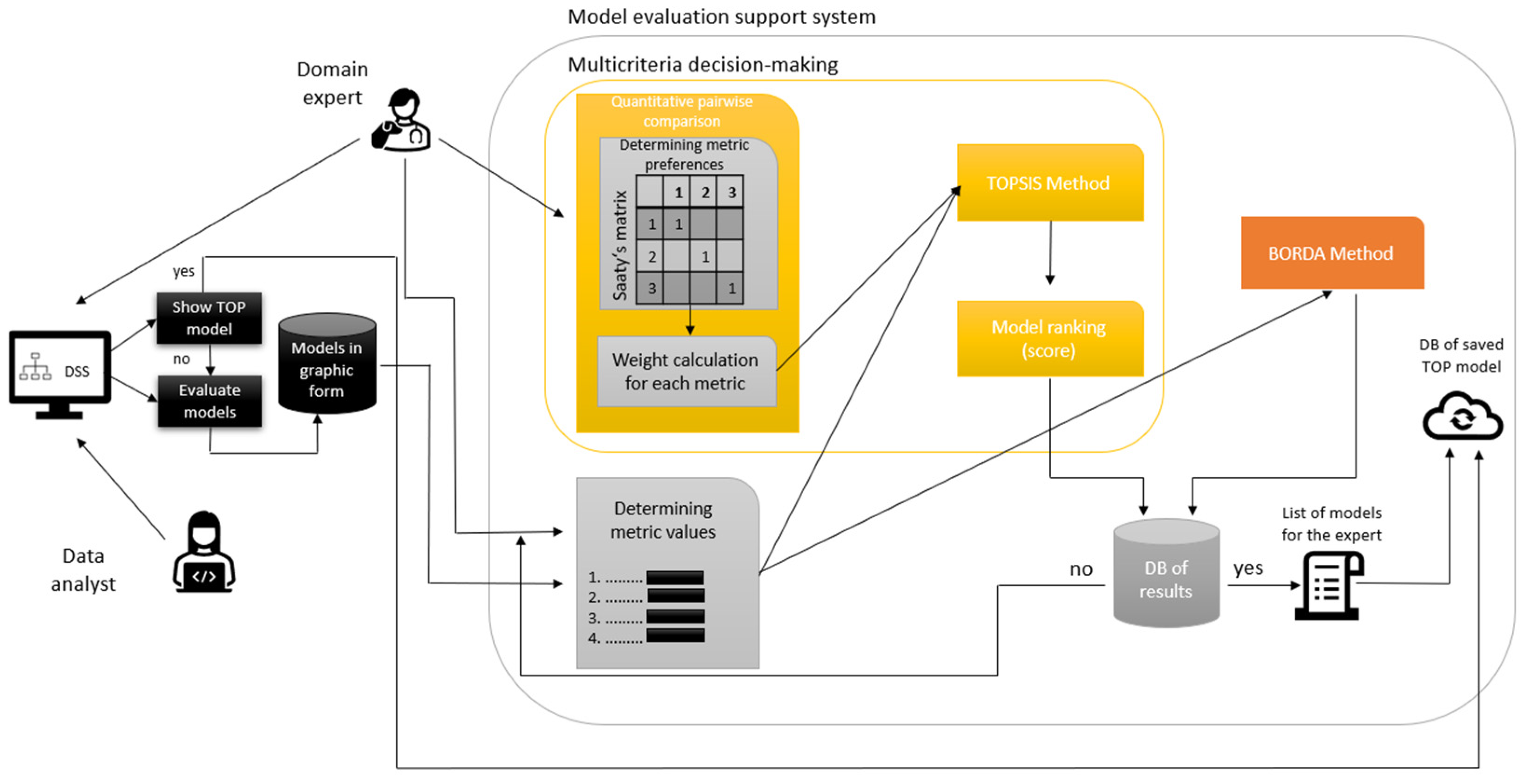
3.1. Proposed Approach

In the second version, this proposal was modified based on communication with participating doctors to achieve better comprehensibility and reduction of diagnostic time. For experimental verification we decided to design a decision support system that would provide the user, the physician, with explanations of predictions, which could improve the understanding of decision models in this area and increase the comprehensibility and trustworthiness of these models with the aim of their use in practice. After displaying individual explanations, physicians should evaluate individual explanations using metrics for evaluating the quality of explanations, with some metrics being calculated automatically and some being evaluated by physicians. Using two evaluation methods and multi-criteria decision-making, the system should finally display the order of models along with explanations in descending order and recommend to the physician which model explanation is the most interpretable, so that during the next use it would save time for physicians and only the model that is most comprehensible would be displayed to them. The prototype of the Clinical Decision Support System for evaluating the quality and comprehensibility of model’s (CDSS-EQCM) was designed and implemented, see Figure 1.

• The user shall show the best model selected and rated by a doctor with many years of clinical experience or generate explainable representations of models in the graphical form in the implemented clinical DSS.
• Subsequently, whether similar models are already stored in the database is checked (DB of saved TOP model).
• If the best model is not stored yet, a domain expert (in our case, a doctor) enters the process.
• The doctor will determine the values of the metrics.
• In the MCDM process, the doctor then determines the metrics preferences of which metric is more important to the other.

  a.

  The doctor chooses preferences between each metric. The values use a scale from 1 to 9, where 1 represents equal importance and 9 represents extreme importance.

• The calculation is performed, the Saaty matrix is filled in, and the weights for each metric are calculated using the normalized geometric diameter of this matrix. The higher the weight, the more critical the metric.
• The values of metrics and metric weights shall be used for calculations performed in the TOPSIS and Borda methods.
• The doctor chooses to evaluate explainable models using the TOPSIS method. Steps in the TOPSIS method:

  a.

  Compilation of the criterion matrix with alternatives (models) as rows and criteria (metrics) as columns. We assign a score (the resulting metric calculation) to each alternative for each criterion.

  b.

  Adjust all metrics to the same extreme type.

  c.

  Normalization of the adjusted criterion matrix.

  d.

  Creating a weighted criterion matrix by multiplying the normalized decision matrix by the weight of each criterion.

  e.

  From the weighted criterion matrix, we determine the ideal and basic models.

  f.

  Finally, we calculate the distance of the model from the ideal model and the basic model, and, using these values, we calculate the relative indicator of the distance of the model from the basic model

• The doctor chooses to evaluate explainable models using the Borda method which is calculated automatically by metaethical formula.
• The system arranges the individual models in descending order.
• The results database will store individual models, model order, values, weights, and preference metrics.
• The doctor will obtain a list of recommended models according to the Borda and TOPSIS methods.
• The doctor will decide whether to save the most understandable model according to the Borda or TOPSIS method or choose his own model that he found most understandable.

3.2. Data Preparation

Preprocessing comprised time-series summarization by transforming each numeric sequence into its first, last, minimum, and maximum values. Binary indicator extraction: parsing free-text notes to flag the presence or absence of clinical events. Auditability retention: preserving original text fields for retrospective validation or advanced NLP processing. The final feature set includes demographics, comorbidities, laboratory and biochemical markers (clotting factors, cardiac enzymes, liver/kidney tests), metabolic and mineral panels, immune profiles (cellular and humoral), blood oxygen saturation (SpO₂), vaccination status, and medication. This curated dataset underpins our subsequent model training and interpretability evaluation. In the first preprocessing phase, we merged Waves 1 and 2 into a single table (1948 × 274), removed free-text and redundant date/order columns, converted Boolean and gender fields to 0/1, recoded vaccine types (0 = unknown, 1 = mRNA, 2 = vector), and let clinicians choose how to impute missing values. We also dropped a discharge-code feature that leaked information about the target (“Severity”). In the second phase, all four waves were combined and metadata “first/last” columns (92 total) and any column with >50% missingness were removed. We restricted the target to a binary outcome (0 = survived, 1 = died), discarded rows with implausible SpO₂ (<45%), and eliminated “transfer” cases. The final dataset comprised 2934 patients and 148 features.

3.3. CDSS-EQCM Development

The CDSS-EQCM prototype was implemented in Python (python-apt—2.4.0+ubuntu1, python-dateutil—2.9.0.post0, python-debian—0.1.43ubuntu1, python-dotenv—1.0.1, python-json-logger—3.3.0) using Streamlit with version of the software 1.15.0 and localized into Slovak for clinicians at UNLP Košice. Development proceeded in two main iterations.

3.3.1. First Version

Data ingestion and preprocessing: Users upload a semicolon-delimited CSV; the system checks for the required “priebeh” (course) column, encodes categorical and Boolean fields to numeric, and stores the cleaned data in session state. Missing-value handling and preview: Clinicians choose to impute with zero, column mean or drop columns; processed data and basic class-based summaries are displayed in collapsible panels. In the first version of the application, we included a dedicated preprocessing step for missing data that allowed clinicians to select one of three strategies before model evaluation: (a) replacing all missing values with zero, (b) imputing with the column mean, or (c) removing any column containing missing entries. By applying the chosen method to the dataset up front, we ensured consistency and transparency in the data preparation pipeline prior to training and interpreting the ML models.

Model evaluation workflow: Physicians select LIME or SHAP, split data, train and evaluate multiple classifiers (accuracy, precision, recall, F1, confusion matrix), then generate local explanations per patient. Interpretability metrics and ranking: In this version, we found that the Identity metric was not applicable, as there were no instances of duplicate records in our dataset. Therefore, applying this metric further would not yield any meaningful results. After computing Separability and Stability, experts rate models on Response time, Understandability, and User Experience. Ratings are saved and aggregated via TOPSIS (with AHP weighting) or Borda count to identify the top model. “Use Best Model” option: Automatically loads the previously selected model, re-evaluates metrics, and presents LIME/SHAP explanations without further configuration.

3.3.2. Second Version

Binary classification adaptation: The target Severity of the disease was recast as survived (0) vs. death (1); transfer cases and implausible SpO₂ values were removed. Interface refinements: we removed the missing-value step, the statistics expander, and the data-splitting controls previously exposed to physicians. We also fixed imputation to the column mean to simplify the interface and guarantee a standardized dataset for all users. Our sensitivity analysis showed that zero-fill, median, and mean imputation shifted model metrics by only 1–2%, making mean-impute a pragmatic and stable default. By consolidating preprocessing, clinicians can devote their full attention to interpreting and evaluating the models rather than managing data-cleaning options. Confusion matrices and LIME/SHAP plots were updated for two-class outputs; explanatory text was streamlined per clinician feedback. Global explainability: A SHAP summary plot was added to visualize feature importance across the entire test set. These iterations delivered a clinician-friendly CDSS-EQCM that supports semi-automated interpretability evaluation and model selection in medical diagnostics.

3.3.3. Classifier Training Details

All five classifiers were implemented in scikit-learn v1.2.2 with the following baseline settings (and random_state = 42 for reproducibility):

• Random Forest (RF): 100 trees (n_estimators = 100), no limit on depth (max_depth = None).
• Decision Tree (DT): default Gini criterion, no pruning.
• Logistic Regression (LR): solver = lbfgs, C = 1.0, max_iter = 1000.
• k-Nearest Neighbors (k-NN): n_neighbors = 5, Euclidean distance.
• Support Vector Machine (SVM): linear kernel, C = 1.0, probability = True.

To optimize each model, we performed a grid search over the most influential hyperparameters using stratified five-fold cross-validation on the training set:

• RF: n_estimators ∈ {50, 100, 200}, max_depth ∈ {None, 10, 20}.
• DT: max_depth ∈ {None, 10, 20}, min_samples_split ∈ {2, 5}.
• LR: C ∈ {0.1, 1, 10}.
• k-NN: n_neighbors ∈ {3, 5, 7}.
• SVM: C ∈ {0.1, 1, 10}.

For each combination, we recorded the mean F1-score and selected the best setting to retrain on the full 80% training split. Final performance metrics (accuracy, precision, recall, F₁) were then evaluated once on the held-out 20% test set, using the same stratified split to preserve class balance. This nested use of stratified splitting and internal cross-validation ensured both robust hyperparameter tuning and stable, reproducible model estimates.

Table 1. Approximate performance results of classifiers for different models.

ML Model	Accuracy	Precision	Recall	F1 Score
RF	0.98	0.97	0.96	0.965
DT	0.97	0.95	0.94	0.945
LR	0.95	0.94	0.94	0.935
k-NN	0.88	0.85	0.88	0.845
SVM	0.95	0.95	0.96	0.950

summarizes each model’s predictive performance on the held-out test set. Random Forest achieved the highest accuracy (98%), followed closely by SVM. K-NN performed more modestly (88% accuracy), reflecting its sensitivity to high-dimensional clinical features. Across models, Random Forest and SVM consistently outperformed simpler classifiers, with mean F1-scores above 0.95. Decision Tree and Logistic Regression yielded competitive results (F1 ≈ 0.94), while k-NN lagged slightly (F₁ ≈ 0.85). These results justify our choice to include a mix of inherently interpretable and black-box models in the explainability evaluation.

In

Table 2. Confusion matrix of classifiers for different models.

Random Forest Confusion Matrix
Real classes		Predicted classes
	0	508	0
	1	12	67
Decision Tree Confusion Matrix
Real classes		Predicted classes
	0	506	2
	1	14	65
Logistics Regression Confusion Matrix
Real classes		Predicted classes
	0	503	5
	1	25	54
k-NN Confusion Matrix
Real classes		Predicted classes
	0	493	15
	1	58	21
SVM Confusion Matrix
Real classes		Predicted classes
	0	497	11
	1	17	62

are the confusion matrices on the 20% hold-out test set (587–588 samples) for each classifier. These matrices confirm that Random Forest and SVM deliver the strongest trade-off between false positives and false negatives, justifying their top rankings in both TOPSIS and Borda evaluations.

3.4. CDSS-EQCM Testing

We performed on-site manual acceptance testing at UNLP Košice with five infectious-disease physicians, using a set of predefined scenarios.

• Test Scenario 1: Evaluating the Interpretability of Explainable Models Using Evaluation Methods.
• Test Scenario 2: Displaying the Best Option from the Previous Evaluation.
• Test Scenario 3: Verification of the Application’s Functionality and Transparency.

Testing occurred in two phases: the first phase uncovered the need for additional data preprocessing, leading to refinement; the second phase validated the fully integrated system locally. The doctors performed the second phase of all three test scenarios, from which we obtained a relevant evaluation of the explainable methods. The doctor reviews all models explained using SHAP and evaluates all the metrics for the SHAP explanation. The metric evaluation results are saved and displayed in

Table 3. Resulting table of metrics evaluated by the doctor.

ML Method	Response Time	Understandability	User Experience	Separability	Stability	Accuracy
RF LIME	1.00	0.80	1.00	1.00	0.76	0.98
RF SHAP	1.00	1.00	1.00	1.00	0.92	0.98
DT LIME	1.00	0.80	0.80	1.00	0.65	0.97
DT SHAP	1.00	1.00	1.00	1.00	0.90	0.97
LR LIME	0.80	1.00	0.80	1.00	0.75	0.95
LR SHAP	0.80	1.00	1.00	1.00	0.92	0.95
k-NN LIME	0.60	0.80	0.60	1.00	0.84	0.88
k-NN SHAP	1.00	1.00	1.00	1.00	0.95	0.88
SVM LIME	0.80	0.80	0.60	1.00	0.55	0.95
SVM SHAP	1.00	1.00	1.00	1.00	0.94	0.95

. We continuously consulted with physicians throughout development. Testing was carried out in several phases; after each phase, we gathered their feedback and integrated all recommendations. Following the final round of testing, we concluded that the system shows strong potential and outlined further enhancements for future work.

When the doctor decided to evaluate using the TOPSIS method an evaluation mechanism was displayed, along with a choice of metric preferences required for multi-criteria decision-making and the Saaty matrix, see

Table 4. Final table—Saaty matrix.

	Separability	Stability	Accuracy	Response Time	Understandability	User Experience
Separability	1.00	0.20	0.14	0.20	0.14	0.14
Stability	5.00	1.00	0.14	0.11	0.11	0.14
Accuracy	7.00	7.00	1.00	3.00	0.33	3.00
Response time	5.00	9.00	0.33	1.00	3.00	5.00
Understandability	7.00	9.00	3.00	0.33	1.00	5.00
User experience	7.00	7.00	0.33	0.20	0.20	1.00

.

Then, the doctor selected the preferred metrics indicating which of the two is more important, and a pairwise comparison is performed. After evaluation, the models table was displayed with weights based on the geometric mean calculation in

Table 5. The resulting weights used in the evaluation calculation by the TOPSIS method.

Metric	Weights
Separability	0.0250
Stability	0.0371
Accuracy	0.2595
Response time	0.2786
Understandability	0.2946
User experience	0.1052

, along with a table of metric values and a list of models ranked in descending order in

Table 6. Resulting model ranking for both methods.

	TOPSIS Method		Borda Count
	Classification Model	Pi Score	Classification Model	Borda Score
1	SVM SHAP	0.9686	RF SHAP	48
2	RF SHAP	0.9525	RF LIME	41
3	k-NN SHAP	0.9413	DT SHAP	38
4	LR SHAP	0.9308	LR SHAP	28
5	DT SHAP	0.9115	DT LIME	27
6	RF LIME	0.6660	k-NN SHAP	27
7	LR LIME	0.4980	SVM SHAP	25
8	k-NN LIME	0.4544	LR LIME	21
9	DT LIME	0.3696	k-NN LIME	9
10	SVM LIME	0.0516	SVM LIME	6

. The model selected by the doctor as the best was saved to the database. In our case, the doctor chose the model identified as the best by the Borda method (Random Forest with SHAP visualization).

The testing revealed that all the actual system responses were identical to the expected system responses. The aim of this testing was to identify any potential system errors and gather feedback from the domain expert, which would allow us to continue our research and consider potential system improvements. Clinicians then completed a 10-item usability questionnaire [47], the System Usability Scale (SUS), rating learnability, transparency, and overall satisfaction, thereby confirming the CDSS-EQCM’s usability and readiness for clinical integration:

• I think that I would like to use this system frequently.
• I found the system unnecessarily complex.
• I thought the system was easy to use.
• I think that I would need the support of a technical person to be able to use this system.
• I found the various functions in this system were well-integrated.
• I thought there was too much inconsistency in this system.
• I would imagine that most people would learn to use this system very quickly.
• I found the system very cumbersome to use.
• I felt very confident using the system.
• I needed to learn a lot of things before I could get going with this system.

The participants completed the SUS: they rated ten items on a five-point Likert scale ranging from “strongly disagree” (1 point) to “strongly agree” (5 points).

For the odd-numbered questions (1, 3, 5, 7, and 9), we summed the scores and then subtracted 5 from the total to obtain (X). For the even-numbered questions (2, 4, 6, 8, and 10), we summed the scores and subtracted that total from 25 to obtain (Y). Finally, we added the two results (X + Y) and multiplied the sum by 2.5 to get the final SUS score. Individual responses of the doctors from the questionnaire are displayed in

Table 7. Individual responses of the doctors from the questionnaire.

	Doctor1	Doctor2	Doctor3	Doctor4	Doctor5
1	5	5	4	4	4
2	2	2	2	2	2
3	4	4	4	4	5
4	2	3	4	4	2
5	5	5	4	3	5
6	1	2	2	2	2
7	4	4	4	5	4
8	2	1	1	2	2
9	4	4	3	4	4
10	2	2	2	2	5

.

We calculated the final SUS score separately for each doctor based on their responses:

$$\begin{gathered} X1=(5+4+5+4+4)-5=17 \\ Y1=25-(2+2+1+2+2)=16 \\ SUS score1=(17+16)\times 2.5=82.5 \end{gathered}$$

The final SUS score for all doctors is shown in

Table 8. Calculation of the final SUS scores for each doctor and the average SUS score.

	Doctor1	Doctor2	Doctor3	Doctor4	Doctor5	Average SUS Score
Odd-numbered	17	17	14	15	17
Even numbered	16	15	14	13	12
SUS score	82.5	80	70	70	72.5	75

.

The variation of the scores between doctors was at standard deviation (±5.2) and range (68–82) for the overall SUS score. Based on the questionnaire responses of SUS, we obtained a score of 75, which indicates good usability. The results confirmed that the system is not only functional and effective but also highly usable, as evidenced by the achieved SUS score of 75. We noted that, while a mean SUS of 75 indicates “good” usability, the observed spread—especially scores below 70—highlights areas for improvement. This suggests that the system is suitable for practical use and has potential for future development.

4. Discussion

Testing the system with doctors at the Clinic of Infectology and Travel Medicine at UNLP in Košice yielded several important insights. The system clearly and comprehensibly determined the chances of survival/death, with the explainable methods selecting the relevant parameters from a medical perspective. The system has practical application potential. The models were well-explained, with each patient having different attributes influencing the prediction. The system operated quickly, and the data were easily understood. The doctors agreed that model explanations using the SHAP method were more comprehensible, and they identified Random Forest as the best machine learning model. This choice was also confirmed by the Borda evaluation method. The doctors concluded that the system has potential for use at the Clinic of Infectology and Travel Medicine. They also proposed recommendations to further improve and streamline the use of the CDSS-EQCM, such as adjustments for specific parameters we can influence (e.g., the medications used) and the option to enter a specific patient currently admitted in the clinic to evaluate his/her prognosis of survival or death.

Based on the extensive development process, system design, and testing by expert physicians, our CDSS-EQCM system has demonstrated strong potential for clinical application. The evaluation process, guided by the CRISP-DM methodology, incorporated both objective metrics and subjective feedback from domain experts. The key findings and practical implications are summarized below.

• System Performance and Accuracy: During testing, all system responses matched the expected outputs, confirming reliability. To prevent overfitting, we held out 20% of the data as an unseen test set (stratified by class) and applied stratified five-fold cross-validation on the remaining 80% for hyperparameter tuning. For each configuration, we tracked the mean and standard deviation of the F₁-score across folds (all σF₁ < 0.02), retrained the best model on the full training split, and then evaluated on the test set. The gap between training and test accuracy was negligible (<0.01—for example, Random Forest achieved 0.98 on both), and precision, recall, and F₁-scores aligned within 1–2%. These low-variance results demonstrate robust generalization without overtraining. Finally, integrating LIME and SHAP enabled transparent identification of key predictive features, further reinforcing confidence in model behavior on unseen data.
• Interpretability and Usability: Physicians evaluated the interpretability of the models using metrics like accuracy, separability, stability, and subjective measures (understandability, user experience, and response time). The multi-criteria decision-making framework—implemented through the TOPSIS and Borda methods—allowed for an ordered ranking of models according to the experts’ preferences. Feedback collected via a questionnaire based on a Likert scale revealed that the explanations provided by the system are clear and comprehensible. In particular, the SHAP visualizations were found to be more intuitive, which was corroborated by the Borda-based ranking.
• Data Handling and Adaptability: The system processed multiple COVID-19 data waves, addressing challenges such as missing values and inconsistent data types through two phases of rigorous preprocessing. The flexible data-handling pipeline ensures that the system can adapt to both synthetic and real patient data, making it applicable for diverse clinical environments. Real data from the UNLP Košice were successfully incorporated after additional modifications, proving the system’s adaptability.
• Workflow Integration and Deployment: Developed using Python and Streamlit, the CDSS-EQCM features a user-friendly interface that facilitates seamless data uploading and preprocessing; interactive model evaluation, including individualized interpretations for selected patients; automatic model ranking and selection based on expert ratings; and the option to use a pre-evaluated “best model” directly, thereby reducing the diagnostic time and effort required from the clinicians. The clear organization of test scenarios and the resultant documentation (supported by figures and tabulated results) demonstrate that the system’s functionalities align well with the clinical decision-making process. This ensures that it can be effectively integrated into current clinical workflows with minimal adjustments.
• Practical Impact and Future Enhancements: The combined objective and subjective evaluations indicate that the system not only supports accurate predictions but also enhances the interpretability and transparency of the results. This builds trust among physicians, enabling them to make informed decisions quickly. As the system saves valuable time by offering the single, most comprehensible model after evaluation, it paves the way for improved patient management and streamlined clinical operations. Based on clinician comments, we identify three key focus areas for future versions to increase the SUS score: streamlining the model-selection workflow, reducing data-loading times for large datasets, expanding inline tooltips and contextual help. Based on SUS sub-scores and qualitative feedback, we pinpoint “ease of operation” (simpler navigation) and “interpretability guidance” (built-in tutorials) as top priorities to boost usability. Future enhancements, informed by ongoing feedback from the clinical community, aim to further tailor the system to specific clinical contexts, extend its functionalities, and ensure robustness in diverse healthcare scenarios.

5. Conclusions

The CDSS-EQCM represents a significant advancement in the application of explainable artificial intelligence for medical diagnostics. Its successful evaluation by experienced physicians and its adaptable, user-centric design underscores its readiness for deployment in clinical practice, where it can contribute to more efficient, transparent, and trustworthy decision-making in patient care.

References

1. Osheroff, J.; Teich, J.; Levick, D.; Saldana, L.; Velasco, F.; Sittig, D.; Rogers, K.; Jenders, R. Improving Outcomes with Clinical Decision Support: An Implementer’s Guide; Routledge: London, UK, 2012; p. 323. [Google Scholar]
2. Sim, I.; Gorman, P.; Greenes, R.A.; Haynes, R.B.; Kaplan, B.; Lehmann, H.; Tang, P.C. Clinical Decision Support Systems for the Practice of Evidence-based Medicine. J. Am. Med. Inform. Assoc. 2001, 8, 527–534. [Google Scholar] [CrossRef] [PubMed]
3. Ribeiro, M.T.; Singh, S.; Guestrin, C. “Why should I trust you?” Explaining the predictions of any classifier. In Proceedings of the ACM SIGKDD International Conference on Knowledge Discovery and Data Mining, San Francisco, CA, USA, 13–17 August 2016; Association for Computing Machinery: New York, NY, USA, 2016; pp. 1135–1144. [Google Scholar] [CrossRef]
4. Lundberg, S.M.; Lee, S.I. A unified approach to interpreting model predictions. Adv. Neural Inf. Process. Syst. 2017, 30, 4766–4775. [Google Scholar]
5. Holzinger, A.; Carrington, A.; Müller, H. Measuring the Quality of Explanations: The System Causability Scale (SCS): Comparing Human and Machine Explanations. Kunstl. Intell. 2020, 34, 193–198. [Google Scholar] [CrossRef]
6. Miller, T. Explanation in artificial intelligence: Insights from the social sciences. Artif. Intell. 2019, 267, 1–38. [Google Scholar] [CrossRef]
7. Arrieta, A.B.; Díaz-Rodríguez, N.; Del Ser, J.; Bennetot, A.; Tabik, S.; Barbado, A.; Garcia, S.; Gil-Lopez, S.; Molina, D.; Benjamins, R.; et al. Explainable Artificial Intelligence (XAI): Concepts, taxonomies, opportunities and challenges toward responsible AI. Inf. Fusion 2020, 58, 82–115. [Google Scholar] [CrossRef]
8. Lee, E.H. eXplainable DEA approach for evaluating performance of public transport origin-destination pairs. Res. Transp. Econ. 2024, 108, 101491. [Google Scholar] [CrossRef]
9. Doshi-Velez, F.; Kim, B. Towards A Rigorous Science of Interpretable Machine Learning. arXiv 2017, arXiv:1702.08608v2. [Google Scholar]
10. Molnar, C. Interpretable Machine Learning. A Guide for Making Black Box Models Explainable; Lulu Publishing: Morrisville, NC, USA, 2019; p. 247. Available online: https://christophm.github.io/interpretable-ml-book (accessed on 16 May 2025).
11. Stiglic, G.; Kocbek, P.; Fijacko, N.; Zitnik, M.; Verbert, K.; Cilar, L. Interpretability of machine learning-based prediction models in healthcare. WIREs Data Min. Knowl. Discov. 2020, 10, 1–13. [Google Scholar] [CrossRef]
12. Gilpin, L.H.; Bau, D.; Yuan, B.Z.; Bajwa, A.; Specter, M.; Kagal, L. Explaining explanations: An overview of interpretability of machine learning. In Proceedings of the 2018 IEEE 5th International Conference on Data Science and Advanced Analytics (DSAA), Turin, Italy, 1–3 October 2018; Institute of Electrical and Electronics Engineers: Piscataway, NJ, USA, 2018; pp. 80–89. [Google Scholar]
13. Carvalho, D.V.; Pereira, E.M.; Cardoso, J.S. Machine learning interpretability: A survey on methods and metrics. Electronics 2019, 8, 832. [Google Scholar] [CrossRef]
14. Yasodhara, A.; Asgarian, A.; Huang, D.; Sobhani, P. On the Trustworthiness of Tree Ensemble Explainability Methods. In Lecture Notes in Computer Science; Springer Nature: Cham, Switzerland, 2021; Volume 12844, pp. 293–308. [Google Scholar] [CrossRef]
15. Luna, D.R.; Rizzato Lede, D.A.; Otero, C.M.; Risk, M.R.; González Bernaldo de Quirós, F. User-centered design improves the usability of drug-drug interaction alerts: Experimental comparison of interfaces. J. Biomed. Inform. 2017, 66, 204–213. [Google Scholar] [CrossRef]
16. Holzinger, A.; Langs, G.; Denk, H.; Zatloukal, K.; Müller, H. Causability and explainability of artificial intelligence in medicine. WIREs Data Min. Knowl. Discov. 2019, 9, 1312. [Google Scholar] [CrossRef] [PubMed]
17. Itani, S.; Rossignol, M.; Lecron, F.; Fortemps, P.; Stoean, R. Towards interpretable machine learning models for diagnosis aid: A case study on attention deficit/hyperactivity disorder. PLoS ONE 2019, 14, e0215720. [Google Scholar] [CrossRef] [PubMed]
18. Wu, H.; Ruan, W.; Wang, J.; Zheng, D.; Liu, B.; Geng, Y.; Chai, X.; Chen, J.; Li, K.; Li, S.; et al. Interpretable machine learning for COVID-19: An empirical study on severity prediction task. IEEE Trans. Artif. Intell. 2021, 4, 764–777. [Google Scholar] [CrossRef]
19. Barr Kumarakulasinghe, N.; Blomberg, T.; Liu, J.; Saraiva Leao, A.; Papapetrou, P. Evaluating Local Interpretable Model-Agnostic Explanations on Clinical Machine Learning Classification Models. In Proceedings of the 2020 IEEE 33rd International Symposium on Computer-Based Medical Systems (CBMS), Rochester, MN, USA, 28–30 July 2020; Institute of Electrical and Electronics Engineers: Piscataway, NJ, USA, 2020; pp. 7–12. [Google Scholar] [CrossRef]
20. Thimoteo, L.M.; Vellasco, M.M.; do Amaral, J.M.; Figueiredo, K.; Lie Yokoyama, C.; Marques, E. Interpretable Machine Learning for COVID-19 Diagnosis Through Clinical Variables. Interpretable Machine Learning for COVID-19 Diagnosis Through Clinical Variables. In Proceedings of the Congresso Brasileiro de Automática-CBA, Online, 23–26 October 2020. [Google Scholar] [CrossRef]
21. Nesaragi, N.; Patidar, S. An explainable machine learning model for early prediction of sepsis using ICU data. In Infections and Sepsis Development; IntechOpen: London, UK, 2021. [Google Scholar]
22. Prinzi, F.; Militello, C.; Scichilone, N.; Gaglio, S.; Vitabile, S. Explainable Machine-Learning Models for COVID-19 Prognosis Prediction Using Clinical, Laboratory and Radiomic Features. IEEE Access 2023, 11, 121492–121510. [Google Scholar] [CrossRef]
23. Gabbay, F.; Bar-Lev, S.; Montano, O.; Hadad, N. A LIME-Based Explainable Machine Learning Model for Predicting the Severity Level of COVID-19 Diagnosed Patients. Appl. Sci. 2021, 11, 10417. [Google Scholar] [CrossRef]
24. ElShawi, R.; Sherif, Y.; Al-Mallah, M.; Sakr, S. Interpretability in healthcare: A comparative study of local machine learning interpretability techniques. Comput. Intell. 2021, 37, 1633–1650. [Google Scholar] [CrossRef]
25. Stasko, J.; Zhang, E. Focus + Context Display and Navigation Techniques for Enhancing Radial, Space-Filling Hierarchy Visualizations. In Proceedings of the IEEE Symposium on Information Vizualization, Salt Lake City, UT, USA, 9–10 October 2000; Institute of Electrical and Electronics Engineers: Piscataway, NJ, USA, 2000; pp. 57–65. [Google Scholar] [CrossRef]
26. Liu, C.; Wang, P. A Sunburst-based hierarchical information visualization method and its application in public opinion analysis. In Proceedings of the 2015 8th International Conference on Biomedical Engineering and Informatics (BMEI), Shenyang, China, 14–16 October 2015; Institute of Electrical and Electronics Engineers: Piscataway, NJ, USA, 2015; pp. 832–836. [Google Scholar] [CrossRef]
27. Rouwendal, D.; Stolpe, A.; Hannay, J. Using Block-Based Programming and Sunburst Branching to Plan and Generate Crisis Training Simulations; Springer: Cham, Switzerland, 2020; pp. 463–471. [Google Scholar]
28. Oceliková, E. Multikriteriálne Rozhodovanie; Elfa: Malmö, Sweden, 2004. [Google Scholar]
29. Maňas, M.; Jablonský, J. Vícekriteriální Rozhodování, 1st ed.; Vysoká škola ekonomická v Praze: Praha, Czech Republic, 1994. [Google Scholar]
30. Fiala, P. Modely a Metody Rozhodování, 3rd ed.; Oeconomica: Praha, Czech Republic, 2013. [Google Scholar]
31. Behnke, J. Bordas Text „Mémoire sur les Élections au Scrutin “von 1784: Einige einführende Bemerkungen. In Jahrbuch für Handlungs-und Entscheidungstheorie; Springer: Cham, Switzerland, 2004; pp. 155–177. [Google Scholar]
32. Paralič, J. Objavovanie Znalost v Databázach; Technická Univerzita v Košiciach: Košiciach, Slovakia, 2003. [Google Scholar]
33. Maimon, O.; Rokach, L. Data Mining and Knowledge Discovery Handbook; Springer: New York, NY, USA, 2010. [Google Scholar]
34. Breiman, L. Random forests. Mach. Learn. 2001, 45, 5–32. [Google Scholar] [CrossRef]
35. Vogels, M.; Zoeckler, R.; Stasiw, D.M.; Cerny, L.C. P. F. Verhulst’s “notice sur la loi que la populations suit dans son accroissement” from correspondence mathematique et physique. Ghent, vol. X, 1838. J. Biol. Phys. 1975, 3, 183–192. [Google Scholar] [CrossRef]
36. Hosmer, D.W.; Lemeshow, S.; Sturdivant, R.X. Applied Logistic Regression; John Wiley & Sons, Inc.: Hoboken, NJ, USA, 2013. [Google Scholar]
37. Cover, T.; Hart, P. Nearest neighbor pattern classification. IEEE Trans. Inf. Theory 1967, 13, 21–27. [Google Scholar] [CrossRef]
38. Fix, E. Discriminatory Analysis: Nonparametric Discrimination, Consistency Properties; USAF School of Aviation Medicine: Dayton, OH, USA, 1985; Volume 1. [Google Scholar]
39. Cortes, C.; Vapnik, V. Support-vector networks. Mach. Learn. 1995, 20, 273–297. [Google Scholar] [CrossRef]
40. Vapnik, V. The Nature of Statistical Learning Theory; Springer Science & Business Media: Berlin/Heidelberg, Germany, 2013. [Google Scholar]
41. Thomson, W.; Roth, A.E. The Shapley Value: Essays in Honor of Lloyd S. Shapley; Cambridge University Press: Cambridge, UK, 1991; Volume 58. [Google Scholar]
42. Velmurugan, M.; Ouyang, C.; Moreira, C.; Sindhgatta, R. Evaluating Fidelity of Explainable Methods for Predictive Process Analytics. In Intelligent Information Systems; Springer: Cham, Switzerland, 2021; pp. 64–72. [Google Scholar]
43. Honegger, M. Shedding light on black box machine learning algorithms: Development of an axiomatic framework to assess the quality of methods that explain individual predictions. arXiv 2018, arXiv:1808.05054. [Google Scholar]
44. Oviedo, F.; Ferres, J.L.; Buonassisi, T.; Butler, K.T. Interpretable and Explainable Machine Learning for Materials Science and Chemistry. Acc. Mater. Res. 2022, 3, 597–607. [Google Scholar] [CrossRef]
45. Joyce, D.W.; Kormilitzin, A.; Smith, K.A.; Cipriani, A. Explainable artificial intelligence for mental health through transparency and interpretability for understandability. npj Digit. Med. 2023, 6, 6. [Google Scholar] [CrossRef] [PubMed]
46. ISO/IEC 25002:2024; Systems and Software Engineering—Systems and Software Quality Requirements and Evaluation (SQuaRE)—Quality Model Overview and Usage. International Organization for Standardization: Geneva, Switzerland, 2024. Available online: https://www.iso.org/standard/78175.html (accessed on 16 May 2025).
47. Brooke, J. SUS: A ’quick and dirty’ usability scale. Usabil. Eval. Ind. 1996, 189, 189–194. [Google Scholar]
Figure 1. CDSS-EQCM.
Applsci 15 07724 g001