Application of Artificial Neural Network (ANN) in Predicting Box Compression Stress (BCS)

Abstract

Box compression strength (BCS) is a critical parameter for assessing the performance of shipping containers during transportation. Traditionally, BCS evaluation relies heavily on physical testing, which is both time-consuming and costly. These limitations have prompted industry to seek more efficient and cost-effective alternatives. This study explores the application of artificial neural networks (ANNs) to estimate BCS at an industry-applicable level. A real-world dataset—covering approximately 90% of the box dimensions commonly used in the industry—was utilized to train a generalized ANN model for BCS prediction. The model achieved a prediction error of approximately 10%. When validated against experimentally measured data from laboratory testing, with single-wall B-flute as a representative, the prediction error was at a much lower level, further demonstrating the model’s reliability. This study offers a novel approach to BCS prediction, providing a cost-effective and scalable alternative to traditional physical testing methods in the packaging industry.

1. Introduction

Corrugated fiberboard packages provide temporary protection for products against damaging forces throughout the distribution process. Among their structural properties, top-to-bottom box compression strength (BCS) is especially critical to the safe distribution and marketing of nearly all consumer goods. Since the invention of corrugated board, BCS has been a central focus of research, with extensive studies exploring the material’s structural behavior during failure.

Over the past 140 years, various methods have been developed to evaluate and improve BCS [1]. Methods for evaluating BCS generally fall into three main categories: analytical modeling, numerical analysis, and mechanical testing [2]. However, each approach has its limitations. The most common formula in analytical modeling is the approach presented by McKee, Gander, and Wachuta in 1963 [3]. The McKee equation is still widely used in the industry due to its simplicity, which makes it very easy and fast to apply in real-world scenarios without the need for additional experiments [4]. However, it has been shown to be inaccurate in many cases, particularly for non-RSC boxes or RSC boxes modified with holes, cutouts, and other design changes [5]. Its limited accuracy is largely due to the wide range of factors influencing BCS, while the McKee equation is a simplified model based on basic corrugated board parameters and empirically derived correction factors [3].

Numerical analysis, most commonly in the form of finite element analysis (FEA), has become the preferred method for predicting BCS, apart from analytical modeling, thanks to its efficiency and robust simulation capabilities, producing reasonable agreement between the model and the limited number of physical samples evaluated [2]. Garbowski, T. et al. applied FEM to estimate the static top-to-bottom compressive strength of simple corrugated packaging by including the torsional and shear stiffness of corrugated cardboard and the panel depth-to-width ratio [6]. Kobayashi, T. predicted corrugated compression strength using FEM by inputting the data of the stress–strain curve obtained by the edge crush test of the corrugated fiberboard [7]. Park, J. et al. investigated the edgewise compression behavior (load vs. displacement plot, ECT, and failure mechanism) of corrugated paperboard based on different types of testing standards and flute types using finite element analysis (FEA) [8], and Marin, G. et al. applied FEM to simulate box compression test for paperboard packages at different moisture levels based on an orthotropic linear elastic material model [9]. However, FEM faces challenges in accurately capturing the anisotropic, nonlinear mechanical behavior of paper-based materials. FEA requires a detailed set of input parameters to simulate stress and displacement, many of which are not regularly measured in the paper-making or box-making process [2]. The additional characteristics such as the humidity dependence of the mechanical properties, creep and hygroexpansion, and the dependency of paper material on time and temperature also makes the material characterization to obtain the input parameters for the FEA even more difficult [10].

Mechanical testing remains the most traditional and reliable method for evaluating BCS. However, it is time-consuming, costly, and destructive—particularly when multiple samples are needed to account for variations in material properties, packaging dimensions, and structural designs—making large-scale evaluations impractical. Furthermore, mechanical testing is constrained by laboratory conditions and equipment limitations, making it challenging to accurately replicate real-world storage and distribution environments. Therefore, more efficient and cost-effective methods are needed to improve the BCS evaluation process.

In recent years, the application of machine learning (ML) in the packaging industry has demonstrated its transformative potential in optimizing operations and enhancing process efficiency. ML offers significant advantages for modernizing traditional packaging practices by increasing automation, improving precision, and supporting data-driven decision-making [11]. Among various ML techniques, artificial neural networks (ANNs) have attracted considerable interest from researchers for their ability to support decision-making and prediction in packaging property evaluations. For instance, Gajewski et al. employed ANNs to predict the compressive strength of various cardboard packaging types by accounting for key influencing factors such as material properties, box dimensions, and the presence of ventilation holes or perforations that affect wall load capacity [12]. Similarly, Malasri et al. developed an ANN model to estimate box compression strength using a limited dataset while considering the effects of box dimensions, temperature, and relative humidity [13]. Gu, J. et al. conducted a comparative analysis to examine the relationships between key ANN architectural factors and model accuracy in the evaluation of BCS [2]. As interest in ANN applications continues to grow, an increasing number of studies have explored its use in packaging evaluation. However, limited research has focused on predicting box compression strength for the diverse box dimensions commonly used in industrial settings. Additionally, it has not been directed toward real-world industrial applications.

This study aims to address that gap by developing an ANN model capable of predicting BCS at an industry-applicable level. Using a real-world dataset covering 90% of commonly used box dimensions in the industry, a generalized ANN model was trained for BCS prediction with a focus on practical industrial applications. During model development, four key ANN parameters—the number of hidden layers, the configuration of neurons per layer, the number of training epochs, and the number of modeling cycles—were optimized using various optimization techniques while balancing the computational efficiency and prediction accuracy of the ANN model. Finally, the model’s reliability was validated using experimentally tested data obtained in the lab, demonstrating the model’s feasibility and potential to significantly advance BCS evaluation methods in the packaging industry.

2. Method

The development of the ANN model involved three main steps. The first step was data preparation. In this study, a real-world industry dataset was curated to represent the majority of box dimensions commonly used in packaging applications for training the ANN model. The second step focused on constructing the ANN architecture by determining key modeling parameters—including the number of hidden layers, the configuration of hidden neurons, the number of training epochs, and the number of modeling cycles —using various algorithms. To optimize the hidden layer configuration, five optimization methods were evaluated, which are detailed later in the study. An exhaustive search [14] was used as a validation technique to assess the effectiveness of these methods and to help identify the global minimum of model error during hidden neuron optimization. To ensure stable and conservative results, the process began with a high initial number of epochs and modeling cycles, followed by iterative refinement until the model error converged. The third step involved verifying the model’s accuracy through physical testing. Figure 1 presents an overview of the analysis process and methodology.

This study involved running programming tasks on an HP Laptop 15t-dy100 featuring an Intel(R) Core(TM) i5-1035G1 CPU, operating at a processing speed of 1.00 GHz. The coding process to train the ANN model was conducted using Jupiter Notebook software 6.5.4, an integrated development environment (IDE).

2.1. Data Collection

To develop a generalized ANN model for BCS evaluation, a real-world dataset [15] of 429 samples, supplied by an industry partner, was initially used. The dataset includes RSC box samples with single-wall construction and flute type A, B, and C [16,17]. Input parameters include the key influencing parameters such as the edge crush test (ECT) values of corrugated board, and box dimensions (Length, width and depth). An industry analysis indicates that the majority of box dimensions typically fall within the following ranges: length between 8 and 25 inches, width between 5.75 and 19 inches, and depth between 4 and 28 inches. These dimensions account for approximately 90% of the boxes sizes used in the industry. Therefore, to ensure the model was trained on a representative subset, only data points within these ranges were selected from the original dataset. The resulting dataset contains 395 data points, and the box parameter details are summarized in

Table 1. Minimum and maximum values of data incorporated into real dataset with 395 data points.

Property	Min	Max
ECT (lbs/inch)	26.13	107.4
Length (inch)	8	25.00
Width (inch)	5.25	19.00
Depth (inch)	5.00	26.50
BCS (lbs.)	347.32	2172.00

. Considering the overall goal of this study—to develop a model capable of predicting BCS for the majority of commercial box dimensions—and the limitations in obtaining input data for validation, the most influential parameter (ECT of the corrugated board) along with the box dimensions (length, width and depth) was selected as the inputs to train the ANN model The output of the ANN was the BCS value.

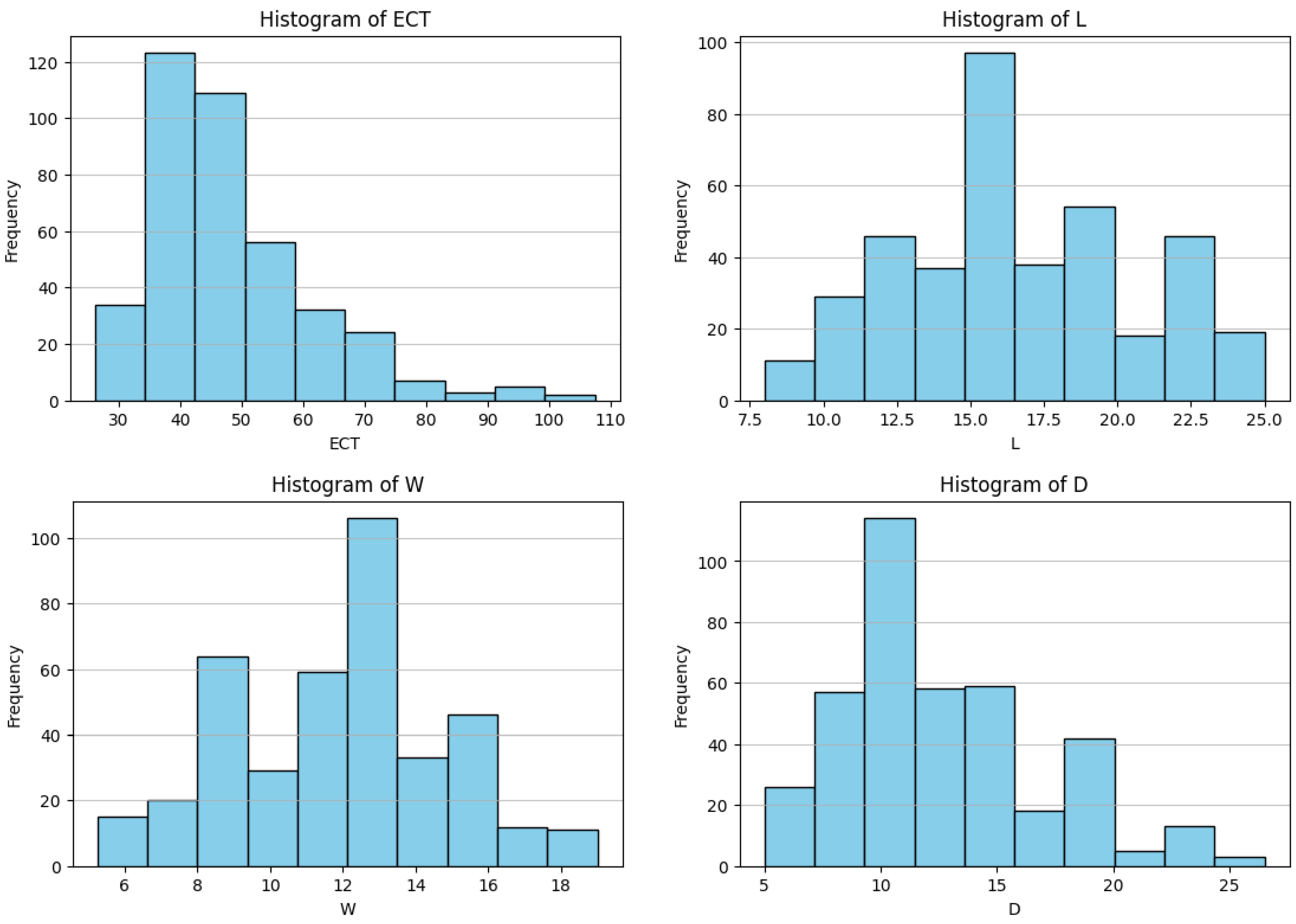
Figure 2 presents histograms of the input features for the extracted dataset with 395 data points, illustrating their data distributions. The histogram for ECT reveals a small portion of data at higher values that may represent outliers. Box depth also shows the slight presence of outliers at the upper end of its range. In contrast, the distributions of box length and width appear relatively uniform and do not exhibit noticeable outliers.

2.2. Development of ANN Model Architecture

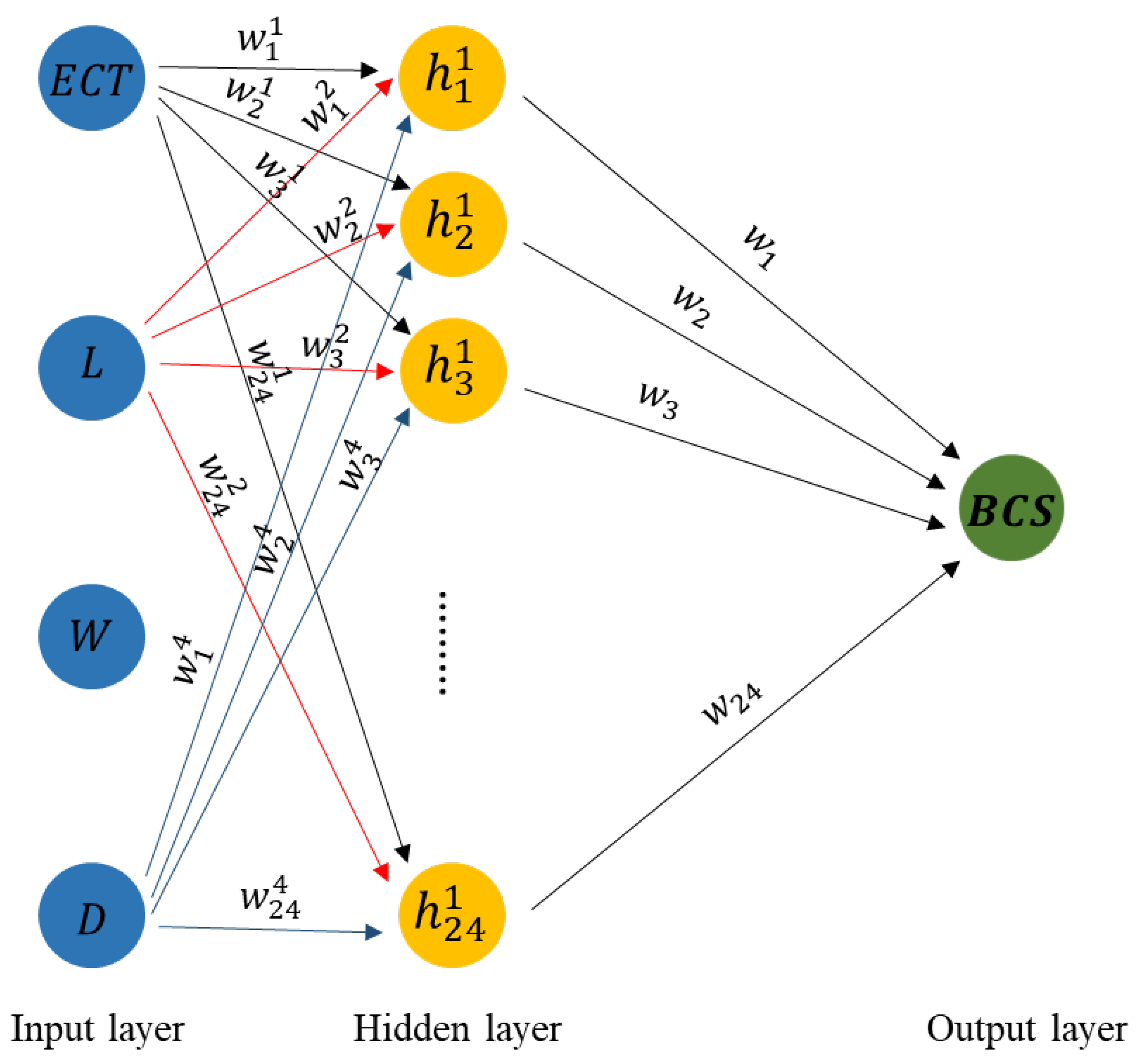
An ANN model is typically composed of three types of layers: an input layer, one or more hidden layers, and an output layer. Since one or two hidden layers are generally sufficient for solving nonlinear problems, this study evaluated models with up to two hidden layers. Figure 3 presents a conceptual diagram of the ANN structure developed in this study.

During the ANN model training process, the dataset was randomly split into two subsets: 70% of the data was used for training the model, and the remaining 30% was reserved for testing the model’s accuracy.

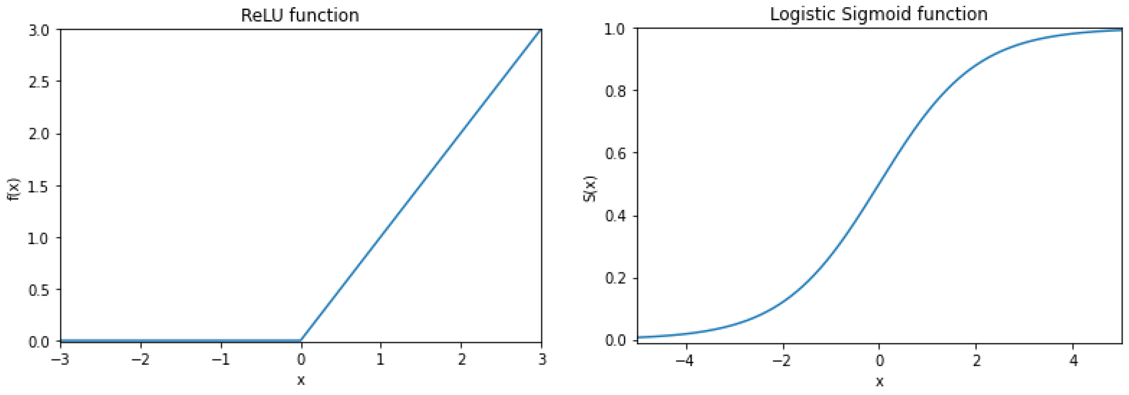
In order to address nonlinear problems and improve computational efficiency, activation functions are commonly employed in ANN models. Typically, different activation functions are used in the hidden and output layers. In this study, the Rectified Linear Unit (ReLU) activation function was applied in the hidden layer [18], while the Sigmoid activation function was used in the output layer [19]. ReLU was chosen for the hidden layer because it helps mitigate the vanishing gradient problem, which often occurs in deep networks with multiple hidden layers, and it enhances computational efficiency by selectively activating a subset of neurons [20]. The Sigmoid function was selected for the output layer because it efficiently produces an output p ∈ [0, 1], which can be interpreted as a probability—an essential feature for the intended prediction task [19]. Plots of the ReLU and Sigmoid functions are shown in Figure 4.

2.2.1. Determination of ANN Hidden Neuron Number Configuration

To construct the ANN model, the hidden layer neuron configuration was determined by balancing model accuracy and computational efficiency. Five optimization methods were evaluated to optimize the hidden layer configuration, aiming to maximize accuracy while minimizing computational cost. The selected optimization methods included the Akaike Information Criterion (AIC) [21], the Bayesian Information Criterion (BIC) [21], Hebb’s rule [22], the Optimal Brain Damage (OBD) algorithm [23,24], and Bayesian Optimization (BO) [25,26]. The number of neurons ranged from 1 to 145, with the number of hidden layers varying from 1 to 2 for the first four methods, and from 1 to 3 for the Bayesian Optimization method. The optimized configurations for the number of hidden neurons, derived from the five methods, were recorded along with the corresponding ANN model’s prediction errors. The final hidden neuron configuration was determined by comparing model errors across all five methods, selecting the configuration that minimized model error while maximizing computational efficiency. An exhaustive search was used as a validation technique to assess the effectiveness of these methods and to help identify the global minimum of model error during hidden neuron optimization. The exhaustive search method not only prevents the model from becoming trapped in local minima of the BCS prediction error but also serves as a reference for balancing model complexity and accuracy, thereby reducing the risk of overfitting.

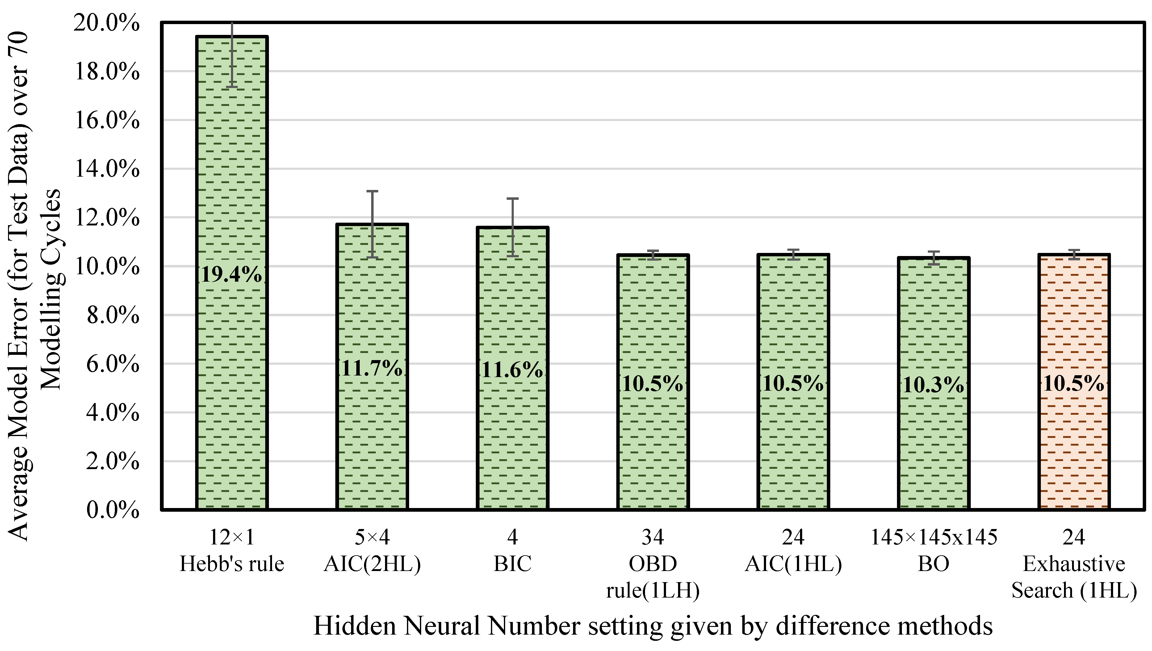
The five methods mentioned above—namely, the AIC, the BIC, Hebb’s rule, the OBD rule, and BO—were evaluated for optimizing the number of hidden neurons in the ANN. The model errors for the test data obtained using each method were calculated and compared, as shown in Figure 5.

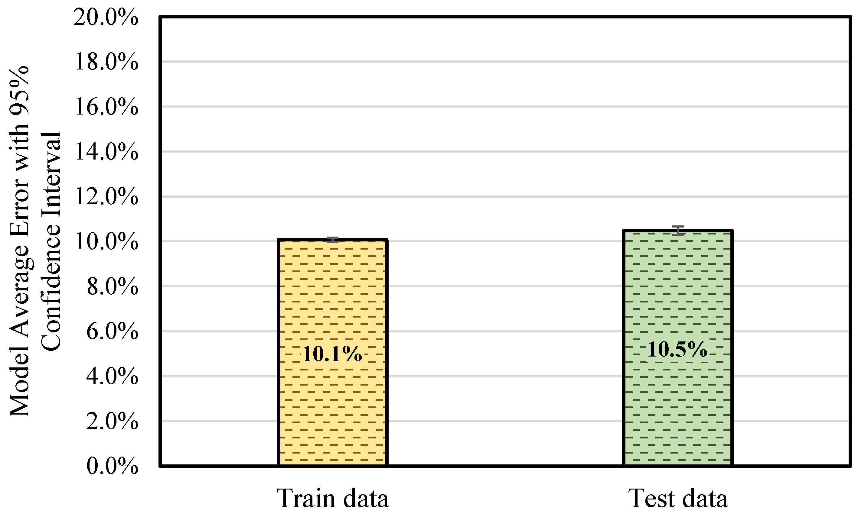
Among the five optimization methods, the Bayesian Optimization approach achieved the lowest model error of 10.3% with three hidden layers, each containing 145 neurons. In comparison, the AIC method (1 HL) produced a slightly higher error of 10.5% using a single hidden layer with only 24 neurons—a significantly simpler architecture. This suggests that increasing the number of neurons to 145 in three layers did not yield a substantial improvement in prediction accuracy over the simpler configuration. To verify this observation, an exhaustive grid search was performed, evaluating hidden layer sizes from 20 to 40 neurons (in increments of 1). The lowest average BCS prediction error of 10.5% was observed with 24 neurons in a single hidden layer, matching the result from the AIC method (1HL), as shown in Figure 5 (the last column). Considering these results and aiming to balance computational efficiency with predictive accuracy, a single hidden layer with 24 neurons was selected as the final optimal ANN architecture, minimizing unnecessary neuron connections.

Based on the research above on ANN architecture, the structure of the generalized ANN model developed for BCS prediction is outlined in Figure 6. The model consists of four BCS features as inputs, featuring one hidden layer with 24 neurons.

2.2.2. Determination of Epoch Number

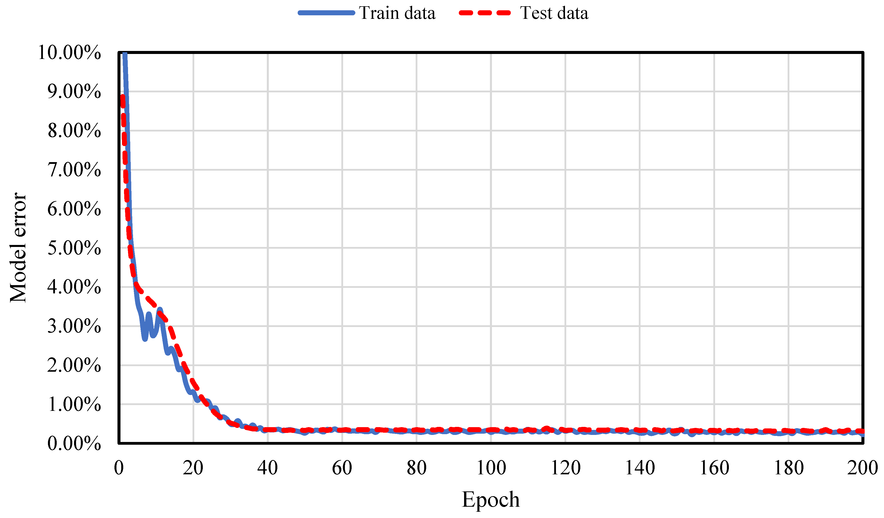
An epoch refers to one complete cycle of training an ANN model, during which the model’s weights are adjusted through both forward and backward propagation. This cycle is repeated multiple times throughout the training process to iteratively improve the model’s performance. The number of epochs plays a crucial role in training, as it directly affects how well the model learns and generalizes unseen data. As a hyperparameter, the number of epochs determines how many times the learning algorithm will process the entire training dataset. Too few epochs can result in an underfit model, while too many can lead to overfitting. In this study, additional epochs were run, and training was stopped once the error converged, optimizing both error minimization and computational efficiency.

After running an additional 200 epochs and calculating the model error (model loss), the results showed that the error for both training and test data began to converge after approximately 40 epochs and remained stable up to 200 epochs. To ensure a conservative result, 50 epochs were selected as the minimum number required to achieve a robust result, as shown in Figure 7.

2.2.3. Determination of Modeling Cycle Number

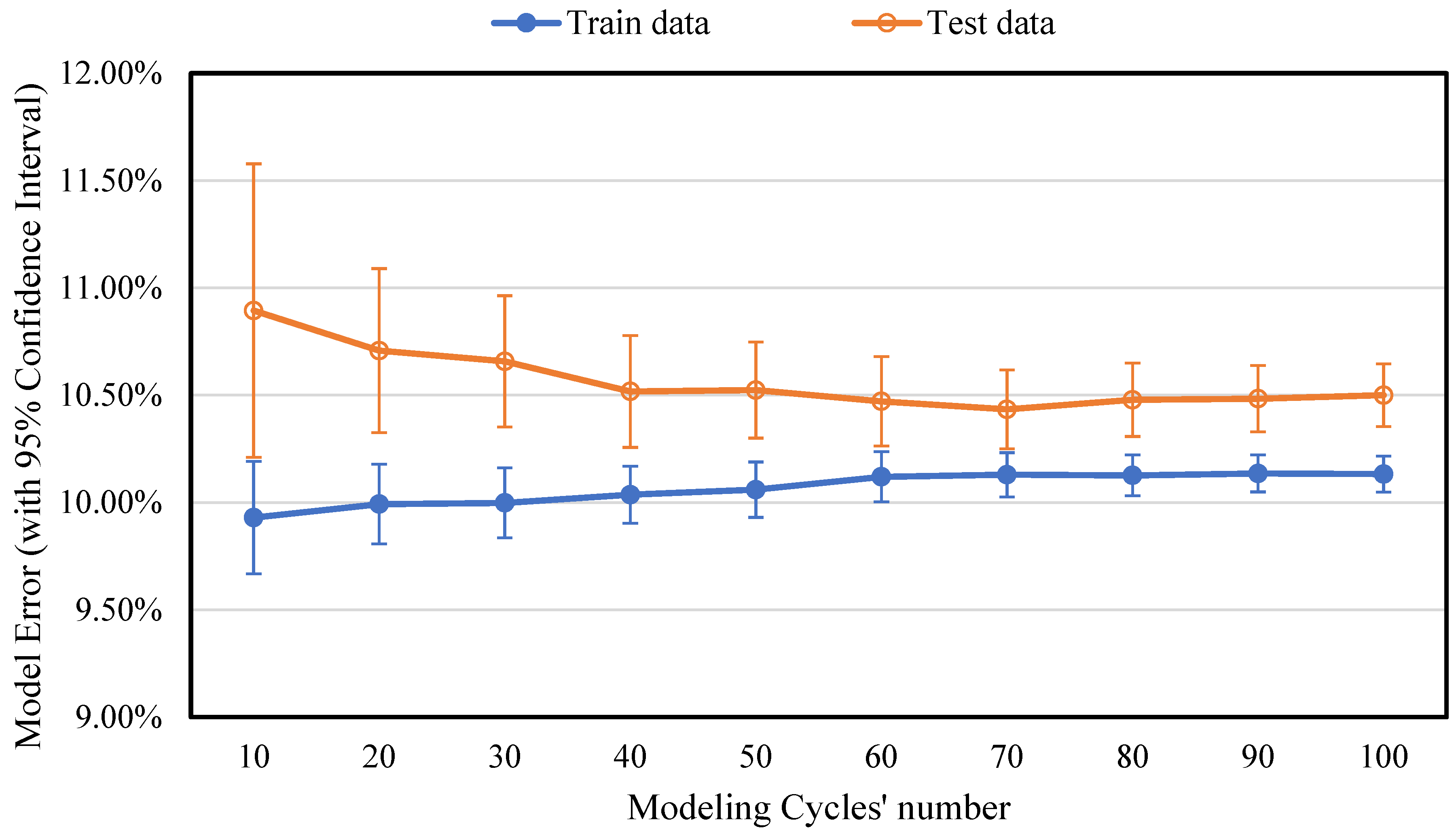
Since ANNs randomly split the data into training and testing sets during the modeling process, each cycle can result in different data partitions. As a result, each cycle may generate a unique model that fits the training data well but produces varying error values when tested on the test data. Therefore, it is crucial to determine how many modeling cycles are needed for the results to converge to a “typical” level of reliability. To investigate the impact of different data partitions on ANN accuracy, various numbers of modeling cycles were tested in this study to ensure model error convergence.

The ANN model was trained with varying cycle counts, ranging from 10 to 100. The model error for each cycle count, along with the 95% confidence interval, was calculated, as shown in Figure 8. The results indicated that the model error for both training and test data converged at 70 modeling cycles. Therefore, a minimum of 70 modeling cycles is required to achieve reliable and consistent results in ANN model training.

A summary of the ANN architecture parameters, including their selection rationale and optimal values, is presented in

Table 2. ANN Architecture Parameters and Rationale for Selection.

ANN Architecture Parameters	Value/Description	Rationale for Selection
Input	ECT	Identified as the most influential parameter affecting BCS
	Length	Included to enable prediction across the majority of commercial box sizes
	Width
	Depth
Hidden layer number	1	Determined via optimization using five different methods and exhaustive search to balance complexity and performance
Hidden neuron number	24
Minimum Epoch number	50	Chosen based on error convergence to ensure stable and robust training
Modeling cycle number	70
Output	BCS	Target variable to be predicted by the ANN model

.

3. Result

The performance of the ANN model was evaluated using the average prediction error of the training and test data across 70 modeling cycles—the number at which the average model error converged—to obtain a conservative result. To comprehensively assess the model’s predictive capability and identify sources of error, the distribution of predicted BCS values was compared with the actual BCS value distribution to reveal the cause of existing errors. Finally, the model’s accuracy was validated using physical test data from 10 commercially sized box dimensions. The validation results demonstrate the model’s reliability for industrial applications, as the validated error was significantly lower than the errors observed in both the training and testing phases.

3.1. Training ANN Model to Evaluate BCS in the Industry

With the extracted data of 395 data points covering the majority box dimensions used in the industry and optimized hidden neuron configuration, epoch number, modeling cycle number, a generalized ANN model was trained to predict BCS at an industrial applicable level. The average BCS prediction error of the training and test data across 70 modeling cycles is 10.1% and 10.5%, respectively, as shown in Figure 9.

Through the standard regression metrics (RMSE, MAE, R²) analysis, it shows the model achieved good predictive performance, with a training MSE of 8908.33, RMSE of 94.38, MAE of 74.91, and coefficient of determination (R²) of 0.896. On the test set, the model maintained high accuracy with an MSE of 11,206.82, RMSE of 105.86, MAE of 82.69, and R² of 0.870. Figure 10 and Figure 11 show parity plots comparing predicted and actual BCS values for the training and test data, respectively. The strong linear correlation and close clustering around the diagonal line in both plots indicate the model’s effectiveness in capturing the underlying relationships between input features and BCS.

To assess the robustness and generalizability of the ANN model, 100 modeling cycles were performed using different random splits of the dataset. The parity plot of predicted versus tested BCS values across these 100 cycles (Figure 11) demonstrates consistently strong agreement, with data points closely aligned along the identity line. This indicates stable model performance and reliable predictive capability across varying data partitions. The overall linear fit observed in the plot further confirms that the ANN model effectively captures the relationship between input features and BCS under repeated training and testing conditions.

To investigate the causes of the BCS error in the ANN model’s predictions, the BCS distribution for two randomly selected modeling cycles was analyzed and plotted, as shown in Figure 12. The actual BCS distribution is represented by the blue columns, while the predicted BCS distributions over 70 modeling cycles are shown in orange. A comparison of the actual and predicted BCS distributions reveals that the model struggles to accurately predict data points with BCS values between 347 lbs and 427 lbs, as well as those between 1999 lbs and 2172 lbs. These values consistently exhibit higher prediction errors compared to other data points. This suggests that boundary data points play a significant role in the high prediction error of the ANN model for BCS evaluation. Boundary points often lie near the edges or outside the range of the training data, resulting in a lack of neighboring data points. While ANNs generally interpolate well within the training range, they tend to struggle with extrapolation, leading to higher errors at the boundaries. Additionally, the data in the boundary regions is relatively sparse among the 395 data points used to train the ANN model. This limited data availability restricts the model’s ability to effectively learn these patterns, thereby contributing to increased prediction errors.

Figure 13 shows the residual distribution histogram for the test data from the ANN model used to predict BCS. The distribution is approximately bell-shaped and centered around zero, suggesting that the model’s prediction errors are symmetrically distributed and generally unbiased, though with a slight positive skew.

3.2. Model Accuracy Verification Using Physical Testing

To further evaluate the capability of the ANN model in predicting BCS values, physical test data from the lab in the School of Packaging at Michigan State University were used to verify the model’s accuracy. The BCS values of 10 single-wall B-flute RCS boxes with varying dimensions, provided by the Packaging Corporation of America (PCA), were measured using a Lansmont Squeezer (S/N 13455) (Monterey, CA, USA). These values were then used as test data for the ANN model that had been previously trained on 395 real-world data samples. For each box dimension, at least 10 samples were tested to calculate the average BCS value, which was used as the representative input for the model. All box samples were preconditioned at a temperature of 23.0 ± 1.0 °C (73.4 ± 1.8 °F) and a relative humidity of 50.0 ± 2.0% for at least 24 h, in accordance with TAPPI T 402, “Standard Conditioning and Testing Atmospheres for Paper, Board, Pulp Handsheets, and Related Products” [27].

Based on the optimal modeling parameters identified above—four inputs (ECT, Box length, Width and Depth), 24 neurons in the hidden layer, and 70 modeling cycles (with the number of epochs extended to 200 epochs for a more conservative result)—the ANN model was further evaluated using BCS data from an additional set of 10 box dimensions tested in the lab. When the BCS data from the 10 box dimensions were used as test data, the model achieved an average prediction error of 3.2% across the 70 cycles—a much lower error rate compared with the test data’s error of 10.5% during the ANN model training process. The results show that the average tested BCS values for all 10 dimensions fall within the range of the minimum and maximum predicted BCS values, as illustrated in Figure 14. These findings suggest that the ANN model can reliably predict BCS for most of the tested box dimensions, demonstrating its accuracy and underscoring its potential for industrial applications. The code used to train the model is provided in Supplementary Python code S1 and S2.

To assess the agreement between the ANN model predictions and the experimentally tested BCS values, a Bland–Altman analysis was performed. The Bland–Altman plot displays the differences between predicted and tested BCS values against their mean. For all the 10 dimensions of the box samples tested, most of the data points fell within the 95% limits of agreement (mean difference ± 1.96 × standard deviation), suggesting good consistency between the model predictions and experimental results. This analysis supports the reliability of the ANN model in predicting BCS values for box samples within the studied range. The Bland–Altman plot of each box sample is shown in Figure 15, from left to right, top to bottom, the box dimensions are: 12 × 8 × 8 in, 16 × 14 × 8 in, 16 × 16 × 8 in, 12 × 12 × 12 in, 14 × 10 × 12 in, 16 × 8 × 6 in, 16 × 10 × 6 in, 16 × 16 × 12 in, 14 × 12 × 10 in, and 12 × 12 × 10 in, respectively.

4. Discussion

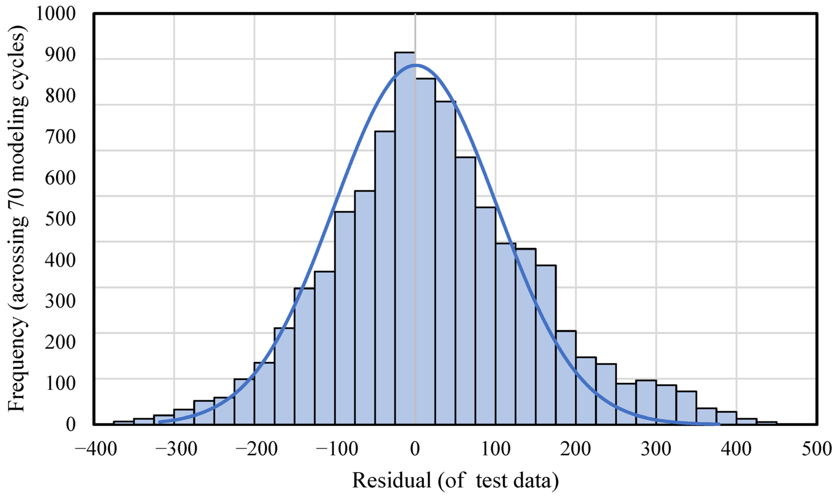
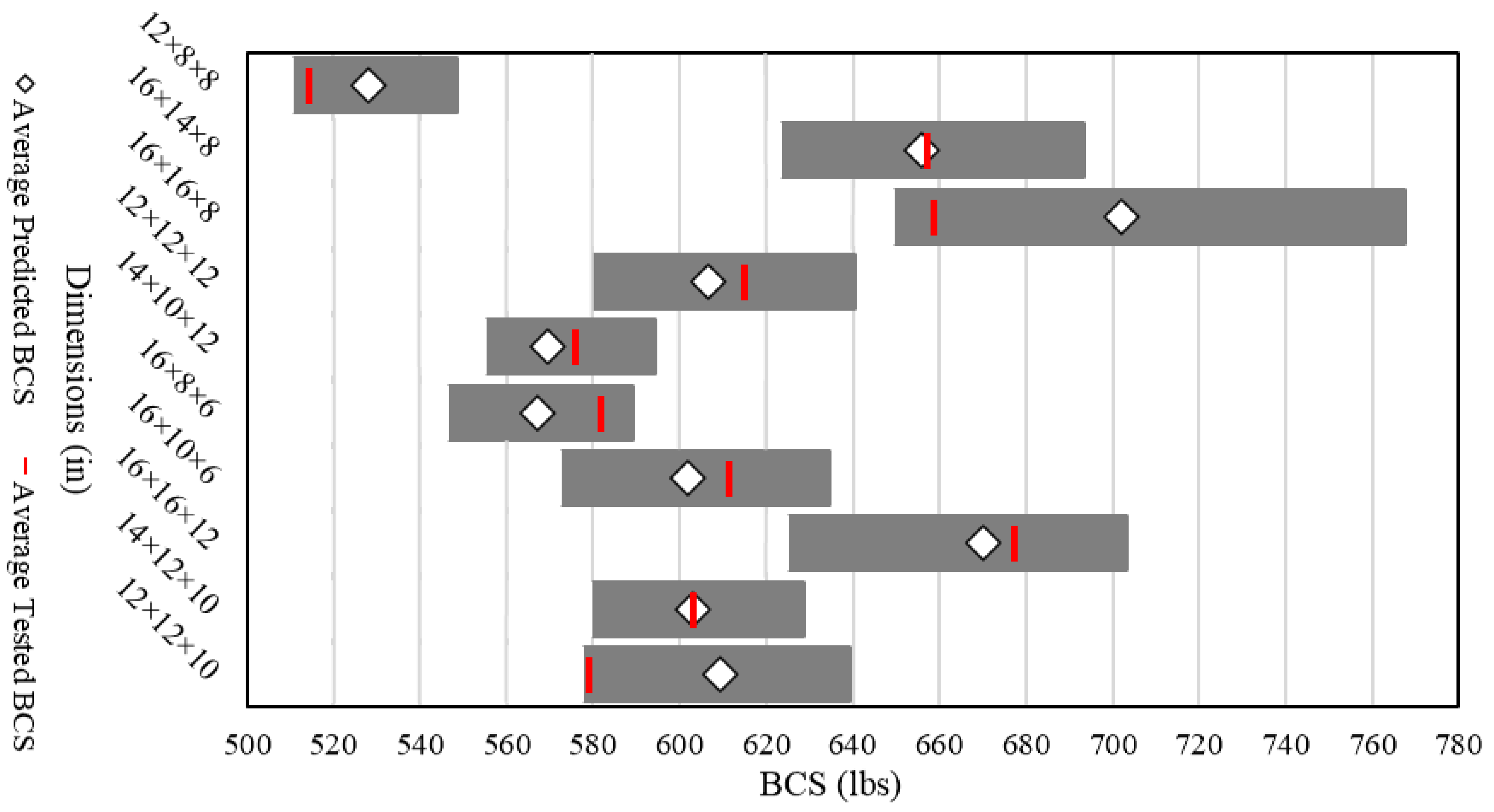
The findings of this study demonstrate the application of ANN models to the real world by predicting BCS values for industrial application. Through training a dataset covering the large majority of box dimensions commonly used in the industry, a generalized ANN model was built with an accuracy level of around 10%. The training results using physically tested data in the lab also demonstrate the accuracy level of the ANN model. The model demonstrates a reliable performance, indicating its suitability for real-world implementation. Overall, this study advances the field in several important and novel ways, beyond the broader dataset coverage:

• Industry-Level Generalization: Unlike prior studies that often focus on limited box types, flute profiles, or experimental conditions, our model is trained on a real-world dataset covering approximately 90% of the box dimensions commonly used in industry. This gives the model practical applicability and scalability not demonstrated in earlier work.
• Systematic Architecture Optimization: Our study introduces a structured, comparative evaluation of five different optimization methods—including AIC, BIC, Hebb’s Rule, Optimal Brain Damage (OBD), and Bayesian Optimization—to determine the ideal hidden neuron configuration. This systematic comparison using exhaustive validation distinguishes our methodological approach from previous works, which often rely on heuristic or single-method tuning.

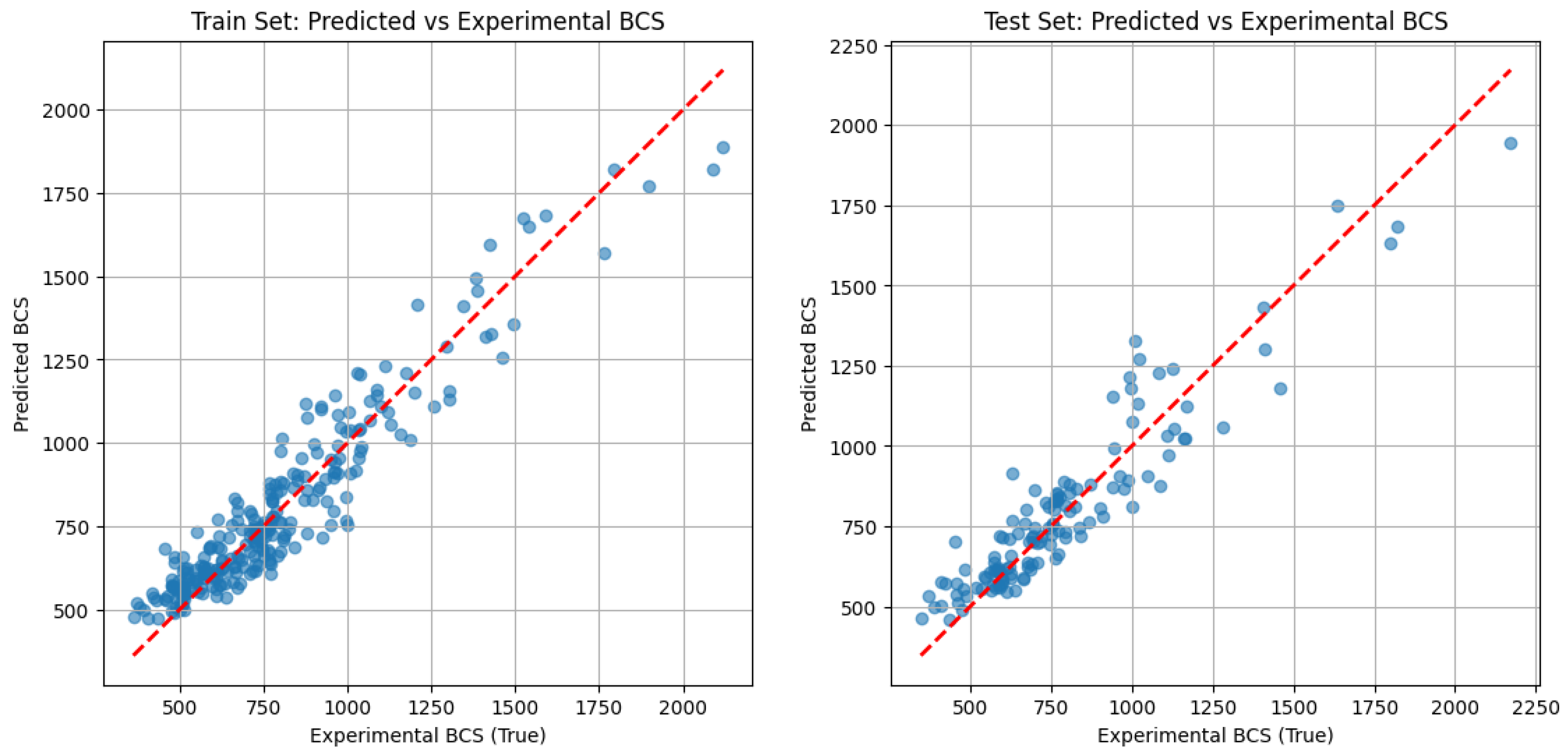
However, the current ANN model has certain limitations. The presence of a residual error can largely be attributed to boundary data points, which introduce variability and potential inconsistencies in predictions. Although the model is trained on a generalized dataset covering 90% of commonly used box dimensions in the industry, the dataset volume remains insufficient—hindering the model’s ability to achieve optimal prediction accuracy. The use of validation data limited to single-wall B-flute boxes may reduce the overall credibility of the validation. Extending the dataset to include other flute types could improve its generalizability and reliability. Furthermore, due to the high cost of generating real-world training data, data collection remains a significant challenge and may require sourcing from multiple avenues, warranting further exploration.

For future studies aiming to improve the accuracy of the ANN model, one key approach is to enhance data quality and expand the dataset. This includes collecting real-world data from diverse sources, such as experimentally validated data from different companies, to increase the model’s reliability and robustness. Additionally, techniques not explored in this study could be employed to further enhance performance. These include data transformation [28,29], which adjusts the distribution of input variables to better align with output targets; data augmentation [30,31], which can improve the model’s robustness; and regularization methods such as weight decay [32,33] and dropout [34,35], which help to improve the generalization ability of the ANN. Moreover, incorporating real-time data and leveraging advanced machine learning techniques—such as reinforcement learning or other deep learning approaches—could further enhance predictive accuracy and optimization, contributing to a more automated and scalable solution for packaging engineering.

To address data scarcity and boundary prediction errors, future work will explore data augmentation techniques to enhance model performance. Approaches such as smooth interpolation between existing samples and regression-adapted SMOTE can generate synthetic data points in underrepresented regions, particularly at BCS extremes. Additionally, small, domain-informed perturbations of box dimensions and ECT values can simulate realistic variability and expand the dataset without requiring costly physical tests. These strategies are expected to improve generalization and reduce prediction error, especially in boundary cases.

5. Conclusions

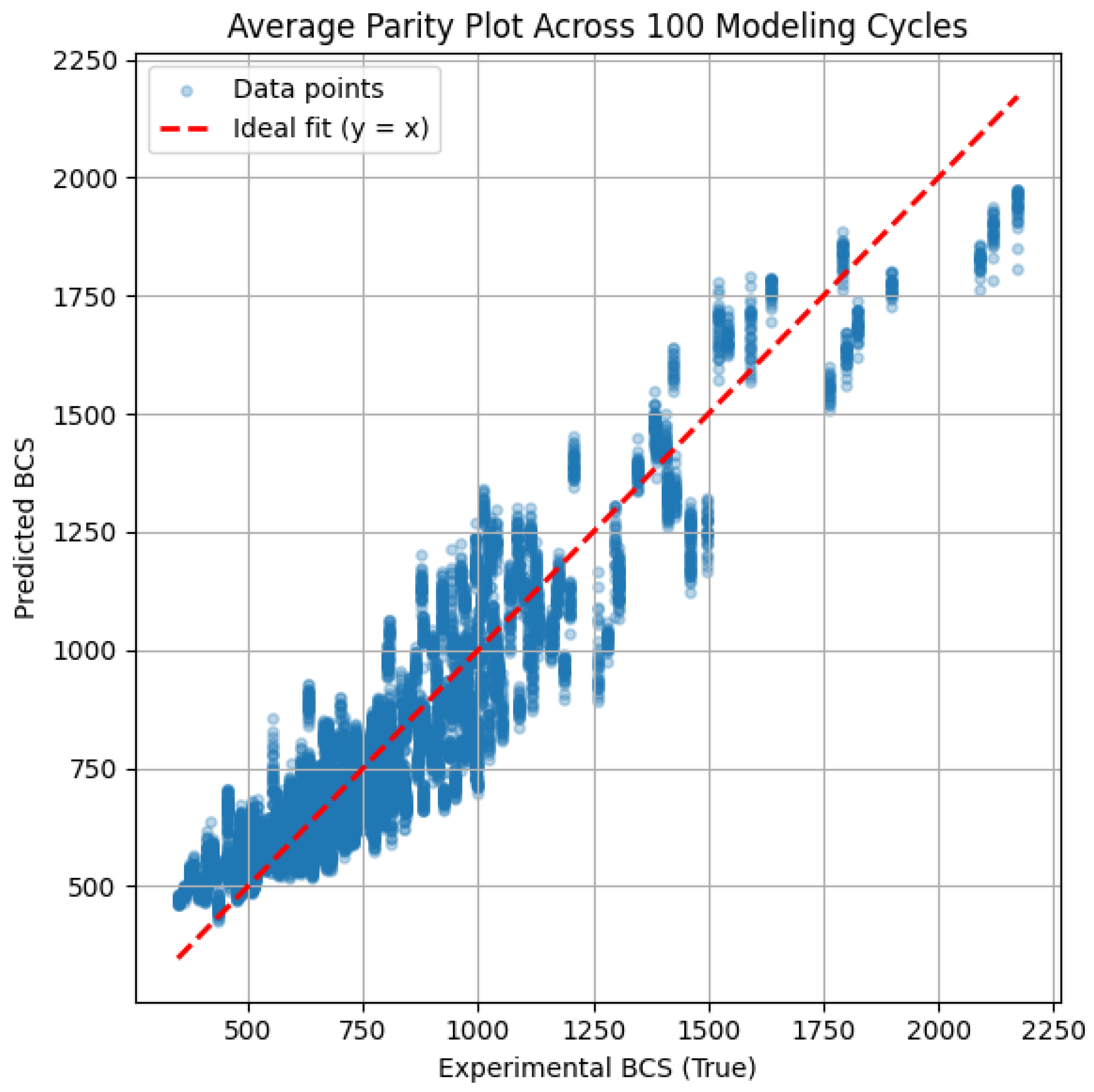
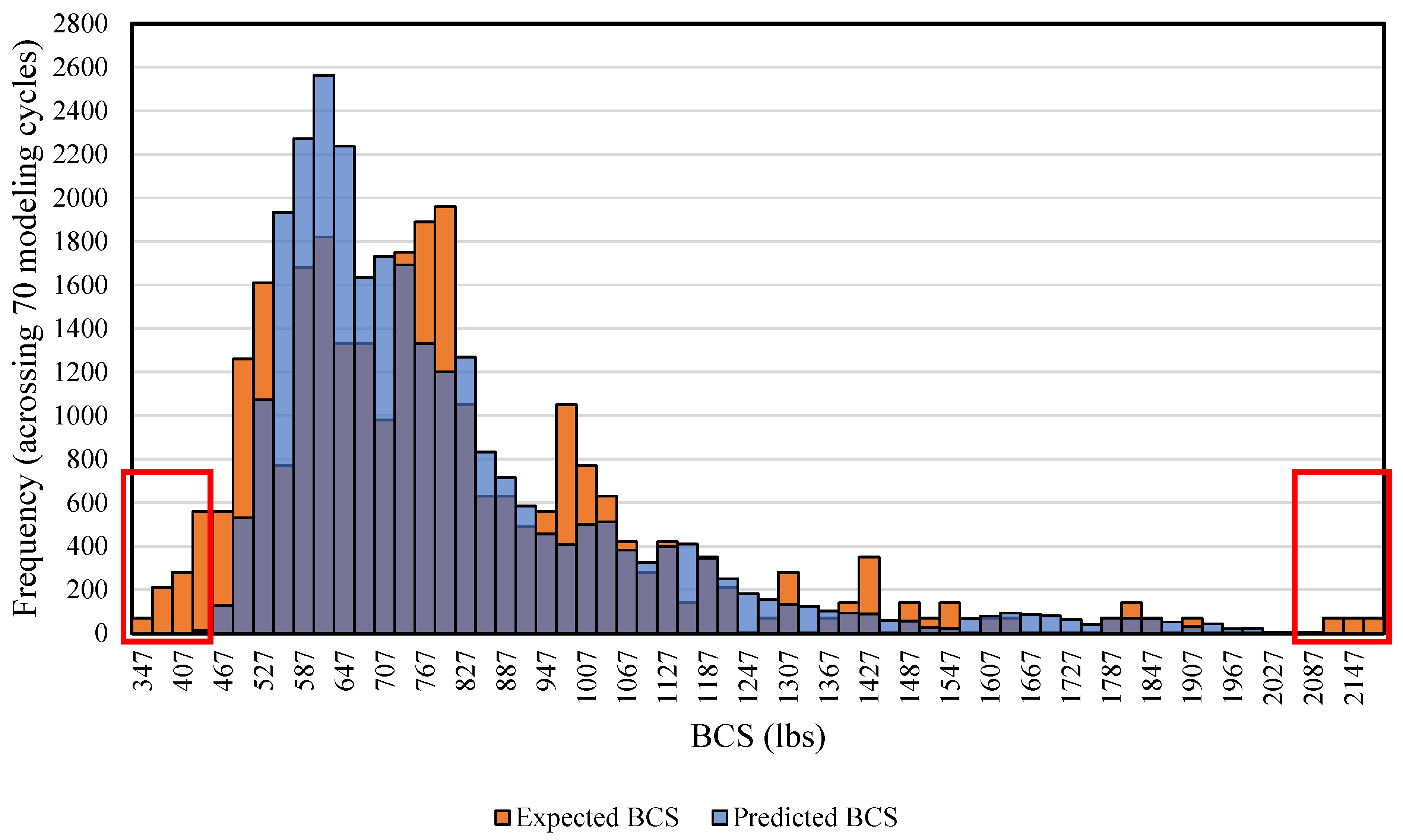
In this study, a generalized ANN model for BCS prediction, designed for industrial applications, was developed. A dataset derived from real-world data was used, covering 90% of commonly used box dimensions in the industry. To optimize the hidden neuron configuration for the ANN model, five methods—the Information Criteria using the AIC method, Hebb’s rule, the Information Criteria using the BIC method, the Optimal Brain Damage rule, and the Bayesian Optimization method—were investigated along with the exhaustive search method. Training results and corresponding model errors were compared to determine the optimal configuration. It was found that a hidden layer with 24 neurons provided the best balance between minimizing model error and reducing computational training time. The optimal epoch number and minimum modeling cycle count were determined to be 50 and 70, respectively, after the training error reduction plateaued. Across 70 modeling cycles, the average BCS error for the test data using the selected configuration was around 10%. Analysis of the BCS value distribution revealed that data points with BCS values between 347 lbs and 427 lbs, as well as those between 1999 and 2172 lbs, consistently showed higher prediction errors. This indicates that boundary data points—those at the extremes of the dataset—are more challenging for the ANN model to predict accurately. Moreover, the limited size of the extracted real-world dataset constrained the model’s overall predictive accuracy. Further research is recommended to expand the dataset and explore data augmentation techniques to enhance the model’s performance. In conclusion, the developed ANN model demonstrates strong capability in predicting BCS values for commonly used box dimensions at an industrially applicable level. It achieved an average prediction error of approximately 10% and was validated by the physical tested data, confirming its practical reliability. This study provides valuable insights into the application of ANN for predicting BCS in corrugated packaging at an industrially applicable level, highlighting its potential to address key challenges in the packaging industry.